| Issue |
A&A
Volume 695, March 2025
|
|
|---|---|---|
| Article Number | A60 | |
| Number of page(s) | 7 | |
| Section | Interstellar and circumstellar matter | |
| DOI | https://doi.org/10.1051/0004-6361/202452875 | |
| Published online | 07 March 2025 | |
Cold molecular gas in the hot nuclear wind of the Milky Way
1
Department of Astronomy, University of Massachusetts,
Amherst,
MA
01003,
USA
2
Dipartimento di Fisica e Astronomia, Universitá degli Studi di Firenze,
via G. Sansone 1,
50019
Sesto Fiorentino, Firenze,
Italy
3
Instituto de Radioastronomía y Astrofísica, Universidad Nacional Autonóma de México,
Apartado Postal 3-72,
Morelia
58090,
Michoacán,
Mexico
4
Black Hole Initiative at Harvard University,
20 Garden Street,
Cambridge,
MA
02138,
USA
5
David Rockefeller Center for Latin American Studies, Harvard University,
1730 Cambridge Street,
Cambridge,
MA
02138,
USA
6
National Radio Astronomy Observatory,
Green Bank,
WV
24944,
USA
7
Research School of Astronomy and Astrophysics, Australian National University,
ACT 2611,
Australia
★ Corresponding author; This email address is being protected from spambots. You need JavaScript enabled to view it.
Received:
4
November
2024
Accepted:
6
February
2025
Abstract
Using the Large Millimeter Telescope and the SEQUOIA 3 mm focal plane array, we have searched for molecular line emission from two atomic clouds associated with the Fermi Bubble of the Milky Way. Neither 12CO nor 13CO J=1–0 emission is detected from the H I cloud, MW-C20. 12CO J=1–0 emission is detected from MW-C21 that is distributed within 11 clumps with most of the CO luminosity coming from a single clump. However, we find no 13CO emission to a 3σ brightness temperature limit of 0.3 K. Using this limit and RADEX non-local thermodynamic equilibrium (non-LTE) excitation models, we derive H2 column density upper limits of (0.4–3)×1021 cm−2 for a set of physical conditions and a H2 to 12CO abundance ratio of 104. Model CO-to-H2 conversion factors are derived for each set of physical conditions. We find the maximum value is 1.6×1020 cm−2/(K km s−1). Increasing [H2/12CO] to 105 to account for photodissociation and cosmic ray ionization increases the column density and X(CO) upper limits by a factor of 10. Applying these X(CO) limits to the CO luminosities, the upper limit on the total molecular mass in MW-C21 is 132±2 M⊙, corresponding to <27% of the neutral gas mass. For the three clumps that are fully resolved, lower limits to the virial ratios are 288±32, 68±28, and 157±39, which suggest that these structures are bound by external pressure to remain dynamically stable over the entrainment time of 2×10⁶ years or are being disrupted by shear and expansion over the clump crossing times of 3–8×10⁵ years. The observations presented in this study add to the growing census of cold gas entrained within the Galactic Center wind.
Key words: ISM: clouds / ISM: molecules / ISM: structure / Galaxy: center / Galaxy: kinematics and dynamics
© The Authors 2025
 Open Access article, published by EDP Sciences, under the terms of the Creative Commons Attribution License (https://creativecommons.org/licenses/by/4.0), which permits unrestricted use, distribution, and reproduction in any medium, provided the original work is properly cited.
This article is published in open access under the Subscribe to Open model. This email address is being protected from spambots. You need JavaScript enabled to view it. to support open access publication.
1 Introduction
Cold gas embedded within hot, outflowing plasma is commonly observed in nearby and distant galaxies (Veilleux et al. 2020). The hot outflowing component is driven by clustered supernovae activity or an AGN-like process of gas accreting onto a supermassive black hole. The presence of cold gas in the hot, expanding plasma is primarily attributed to the entrainment of neutral atomic and molecular clouds that were originally located within the wind’s expansion cone in the central region of the galaxy (Aalto et al. 2012; Walter et al. 2017). An alternative explanation is in-situ formation of cold gas by the condensation of hot gas and the development of thermal instabilities from which atoms and molecules can emerge (Thompson et al. 2016).
Such multi-phase winds have an important role in the evolution of galaxies. The radiative and mechanical feedback can suppress star formation activity where the wind interacts with the cold, neutral gas of the galaxy. The extreme conditions of the entrained neutral gas are likely unsuitable for producing new stars. This suppression of star formation activity by feedback processes can account for the observed decrements of the galaxy luminosity function relative to theoretical expectations (Silk & Mamon 2012). The decrement at the low end of the luminosity function is attributed to supernova feedback while AGN activity may be responsible for the decrement at the high end of the luminosity function.
The Fermi Bubble is a nearby example of an energetic galactic wind likely powered by an accretion event onto the massive Sgr A* black hole (Su et al. 2010). It is comprised of two symmetric plumes of hot electron gas that extend 10 kpc above and below the disk. Heywood et al. (2019) found bipolar, non-thermal radio emission at 1.3 GHz that extends 240 pc below the plane and 190 pc above the plane. X-ray emitting lobes are located at the base of the plumes that indicate a secondary, lower energy outflow likely driven by the super star clusters in the central 200 pc of the Milky Way (Ponti et al. 2019; Nakashima et al. 2019). In projection, neutral, atomic clouds are observed within the boundaries of the Fermi Bubble that indicate a multiphase galactic wind (McClure-Griffiths et al. 2013; Di Teodoro et al. 2018). Recent maps of 12CO J=2–1 emission have identified molecular gas clouds within the domains of two compact, atomic clouds (MW-C1 and MW-C2) and demonstrate that the multiphase outflow includes molecular gas (Di Teodoro et al. 2020). A larger census of molecular line emission has been made in 17 additional atomic clouds (MW-C3 to MW-C19) (Di Teodoro, in prep.).
The multi-phase wind in the Milky Way affords an opportunity to investigate this hot-cold wind phenomenon with high spatial resolution. Specifically, H I 21 cm and CO spectroscopy can establish radial velocities of the entrained gas and a more detailed view of the cold gas kinematics. From the spectroscopic data, we can compile gas properties of the entrained clouds that can be compared to cold, neutral clouds located in the disk to assess the impact of the local environment on the gas conditions.
In this program, we extend the search for molecular gas in the Fermi Bubble by mapping 12CO and 13CO J=1–0 emission from the atomic gas clouds G1.7+3.7−234 (hereafter, MW-C20) and G358.7+3.7+179 (hereafter, MW-C21) that are identified in a blind survey of H I 21cm line emission over the areas 0◦ ≤ |l| ≤ 10° and 3° ≤ |b| ≤ 10° using the Green Bank Telescope (GBT) (Di Teodoro et al. 2018). These 2 clouds are selected from this compilation on the basis of having H I column densities greater than 1.5×1019 cm−2 and compact, centrally condensed atomic gas distributions as measured by the 9′ half-power beam width (HPBW) of the GBT. MW-C20 was first identified in this survey. MW-C21 was originally identified in the HIPASS survey that applied a new algorithm to search for high velocity clouds (Putman et al. 2002) and is also included in the compilation of atomic clouds by Di Teodoro et al. (2018). Within this sample, MW-C21 stands out as having the largest H I 21 cm full width half maximum (FWHM) line width of 41 km s−1. In this study, we adopt distances of 7.62 kpc and 8.53 kpc for MW-C20 and MW-C21 that are based on the simplified, kinematic wind model of Di Teodoro et al. (2018), which accounts for the displacement off the Galactic plane and distance from the Galactic Center.
2 Data
Observations of 12CO and 13CO J=1–0 emission were obtained simultaneously with the 50 meter Large Millimeter Telescope (LMT) Alfonso Serrano in June 2023 and March, April, and August 2024 using the 16 element focal plane array receiver SEQUOIA. The half-power beamwidths of the telescope at the line rest frequencies for 12CO (115.2712018 GHz) and 13CO (110.2013541 GHz) are 12″ and 13″ respectively. The Wide-band Array Roach Enabled Spectrometer (WARES) was used to process the spectral information using the configuration with 400 MHz bandwidth and 97 kHz per spectral channel, which provides a velocity resolution of 0.25 km s−1 for 12CO and 0.27 km s−1 for13 CO. Data were calibrated by a chopper wheel that allowed switching between the sky and an ambient temperature load. The chopper wheel method introduces a fractional uncertainty of ∼10% to the measured antenna temperatures (Narayanan et al. 2008). Routine pointing and focus measurements were made to ensure positional accuracy and optimal gain.
To cover the 15′×15′ area for each target cloud, we observed 4 submaps each covering 7.5′×7.5′ using On-the-Fly (OTF) mapping with scanning along the Galactic longitude axis. All data were processed with the LMT spectral line pipeline package, lmtoy (Teuben et al. 2024), which included calibration by the system temperature, zero-order baseline subtraction, and grid-ding of the spectra into a spectral line data cube, weighted by both a spatial jinc function kernel and 1/σ2, where σ is the root mean square of antenna temperature values in velocity intervals where no signal is expected. The spatial pixel size of the data cube is 5.5″, which approximates the Nyquist sampling rates for imaging 12CO J=1–0 and 13CO J=1–0 emission. The data are spectrally smoothed and resampled to 1 km s−1 resolution and channel width. A main-beam efficiency of 0.6 is applied to convert the data from the  temperature scale to main-beam temperatures, Tmb. The median rms sensitivities in main-beam temperature units at 1 km s−1 resolution are: 0.18 K (12CO) and 0.11 K (13CO) for MW-C20 and 0.15 (12CO) and 0.10 (13CO) for MW-C21. In sections where the 4 submaps overlap, the rms values are lower by ∼20% relative to these median values.
3 Results
The compiled 12CO and 13CO spectroscopic maps of MW-C20 and MW-C21 enable a search for molecular gas within the velocity range of the H I 21 cm line emission. For MW-C20, the H I 21 cm line emission covers the velocity range of [−260,−200] km s−1 with the strongest emission between [−250,−220] km s−1. There is secondary H I velocity component in the observed field that ranges from −160 km s−1 to −110 km s−1 that spatially overlaps with MW-C20. The H I emission from MW-C21 spans the velocity interval 130 to 225 km s−1 with the brightest emission between 150 and 190 km s−1. Figure 1 shows the column density maps of atomic gas from Di Teodoro et al. (2018), 12CO and 13CO J=1−0 maps of integrated intensity for both clouds over the velocity intervals [−250,−220] km s−1 for MW-C20 and [150,190] km s−1 for MW-C21. For MW-C20, 12CO and13 CO velocity integrated emission is not detected to 3σ limits of 3.0 and 1.8 K km s−1 respectively. Nor is either transition found in the secondary velocity component between −160 km s−1 and −110 km s−1. 12CO emission is detected in several regions within the MW-C21 atomic cloud. However, we find no detected13 CO velocity integrated emission to a 3σ limit of 1.9 K km s−1.
An examination of the MW-C21 12CO spectra shows there are several distinct velocity components within the cloud. The FWHM line widths are much narrower than the velocity interval over which the spectra are integrated. This introduces excess noise to the spectra that can limit the detection of CO emission. To improve the signal to noise ratio (S2NR), the 12CO J=1−0 data cube is segmented into islands of detected emission using the pycprops module, which is a python implementation of the cprops package (Rosolowsky & Leroy 2006). The root mean square (rms) is calculated for channels outside of the velocity interval [130, 190] km s−1 for each pixel. A S2NR data cube is generated by dividing the brightness temperature in each velocity channel by its rms value for all spatial pixels. Islands (hereafter, clumps) are identified based on the 3-dimensional connectivity of neighboring spatial pixels and velocity channels with signal to noise ratios greater than 1.5. The choice of the S2NR threshold of 1.5 allows us to recover faint signal with respect to our sensitivity. To reduce the probability of false positive identifications, we also require that an island have at least 3 connected spectral channels that satisfies the S2NR threshold for each spectrum and be comprised of 4 or more spatial pixels. The probability of a random value sampled from a normal distribution being greater than 1.5σ is 0.067. The probability that 3 contiguous channels exceed 1.5σ is (0.067)3 =0.0003. The 4 spatial pixel minimum criterion further decreases the false positive probability. The clumps are not decomposed further into smaller objects.
Applying this segmentation method to the MW-C21 12CO data, 11 molecular clumps are identified in the observed field. This decomposition provides a more precise, customized velocity interval over which there is detected CO emission to improve the signal to noise of integrated intensity at the native 12″ angular resolution for each labeled clump. The location and integrated intensity of the clumps are displayed in Figure 2. The average spectra over the solid angle of each clump are shown in Figure 3.
We have further searched for 13CO emission from MW-C21 by applying the 12CO-derived masks to the 13CO data cube for each clump. Despite the reduction of noise given the customized velocity interval, 13CO emission is still not rigorously detected in any of the clumps.
The pycprops module derives properties of the detected clumps. The calculation for each parameter is summarized by Rosolowsky & Leroy (2006). Table 1 lists the number of position-position-velocity (ppv) voxels, the positional centroid coordinates and centroid radial velocity, velocity dispersion (temperature weighted second moment), equivalent circular radius that matches the clump area, and CO luminosity. For the velocity dispersion, spatial moments (σr,ma j, σr,min), and CO luminosity, pycprops applies a correction to account for sensitivity bias. Rosolowsky & Leroy (2006) provide a detailed description for computing this correction. The extrapolated spatial moments are deconvolved with the telescope beam dispersion width, σbeam,
![Mathematical equation: ${\sigma _r} = {\left[ {{{\left( {\sigma _{r,maj{\rm{ }}}^2 - \sigma _{beam{\rm{ }}}^2} \right)}^{1/2}}{{\left( {\sigma _{r,min{\rm{ }}}^2 - \sigma _{beam{\rm{ }}}^2} \right)}^{1/2}}} \right]^{1/2}}$](/articles/aa/full_html/2025/03/aa52875-24/aa52875-24-eq2.png) (1)
(1)
(Rosolowsky & Leroy 2006). Clumps with σr,min < σbeam are considered unresolved. Uncertainties for several of the clump properties are derived within the pycprops package using the bootstrapping method in which a randomly selected subset of the full data sample are used to derive a given property (Efron 1979). This is repeated 128 times to generate a distribution of values from which confidence levels are determined.
The most conspicuous feature identified in the MW-C21 12CO data is Clump 2, which exhibits the largest size, velocity dispersion, and CO luminosity. Figure 4 shows the integrated intensity and velocity centroid images of Clump 2 and the adjacent Clump 1. While identified as a distinct object, Clump 1 is likely an extension of Clump 2 as its radial velocity smoothly extends the systematic shift from higher radial velocities in the lower right section of Clump 2 to lower velocities in the upper left section. Measured end-to-end from Clump 2 to Clump 1, the radial velocity gradient is 1.3±0.4 km s−1 pc−1. Added together, Clump 1 and Clump 2 comprise 73% of the detected CO luminosity within the field.
The pycprops algorithm was similarly applied to the MW-C20 12CO J=1−0 data to search for any signal that could be diluted by excess noise in the integrated intensity image in Figure 1. With a signal to noise threshold of 1.5, no 12CO emission could be found.
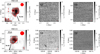 |
Fig. 1 Images of atomic hydrogen column density, 12CO and 13CO integrated intensities for (top row) MW-C20 and (bottom row) MW-C21. The N(H I) contour levels are (0.5, 1, 1.5)×1019 cm−2 and (1, 2, 3, 4)×1019 cm−2, respectively. While 12CO emission is visible in several regions of MW-C21, the broad velocity range with respect to the narrow velocity components dilutes the signal with excess noise. No 13CO J=1−0 emission is detected in either cloud. The red circles show the GBT half power beam width of the HI observations. The red circles in the lower right corner of the middle and right images denote the half power beam widths at 12CO and 13CO. |
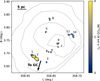 |
Fig. 2 Image of 12CO integrated intensities of clumps in MW-C21 based on the 3 dimensional mask array that identifies islands of connected CO emission. The dotted contours show the distribution of atomic hydrogen column density with contour levels (1, 2, 3, 4)× 1019 cm−2. |
4 Discussion
4.1 Comparison of MW-C21 to MW-C1 and MW-C2
The observations described in this study contribute one more example to the 2 targets previously identified by Di Teodoro et al. (2020) that contain molecular gas within atomic clouds linked to the Fermi Bubble. A comparison of MW-C21 to these 2 clouds offers insight to the origin and nature of molecular gas in these environments.
Morphologically, Clumps 1 and 2 form an extended wall of molecular gas within the MW-C21 atomic cloud that is oriented perpendicular to the direction of the Galactic Center and presumably, the flow direction of the hot wind. This orientation is similar to MW-C1 described by Di Teodoro et al. (2020) and may be a signature to a cloud-wind shock front. Beyond this molecular gas wall, the remaining clumps are very compact and distributed downstream from Clumps 1 and 2. This is similar to the 12CO distribution found in MW-C2.
Kinematically, the 12CO velocity centroids of MW-C21 range from 142 to 185 km s−1 that are distributed in 2 distinct velocity intervals over a physical scale of 24 pc. The higher velocity clumps with VLSR > 1754 km s−1 are compact and located downstream from Clump 2 along the direction to the Galactic Center and presumably, the wind flow direction. This configuration suggests that the higher velocity clumps have been ablated from the largest molecular clump and accelerated by the galactic wind. MW-C2 also shows 2 velocity components that span 30 km s−1 over ∼20 pc scale and CO emission oriented along the direction to the Galactic Center. For the individual velocity components in MW-C21, the velocity dispersions are between 0.9 and 4.5 km s−1. For comparison, the velocity dispersions are ∼1 km s−1 for MW-C1 and 2–5 km s−1 in MW-C2. The velocity gradient identified in the composite velocity centroid image of Clumps 1 and 2 indicates the presence of large scale velocity shear across the clump. Velocity gradients are also found in MW-C1 and MW-C2 but are more localized.
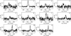 |
Fig. 3 Coadded average 12CO J=1−0 spectra for each molecular clump in MW-C21 based on the 3 dimensional mask array. |
Properties of molecular clumps in MW-C21.
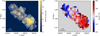 |
Fig. 4 Images of 12CO (left) integrated intensities and (right) centroid velocities that combine the masks for Clump 1 and Clump 2. The contours show the distribution of 12CO integrated intensities with levels 1, 3, 5, 7, 9 K km s−1. |
4.2 Clump masses
Accurate values for the atomic and molecular masses are required to evaluate the dynamical state of the neutral gas. Atomic gas column densities are derived from the integrated intensity of the H I 21 cm emission over the cloud velocity interval, N(H I) = 1.823×10¹⁸ ∫ TB,HI(v)dv cm−2 that assumes optically thin emission. The atomic mass of the cloud, M(H I) = µHmHD2 ∫ N(HI) dΩ, where D is the distance to the cloud, µH is the mean atomic weight = 1.4 to account for the contributions from He, mH is the mass of the hydrogen atom, and the integration is over the solid angle of H I emission. The masses of atomic gas within the 0.5×1019 cm−2 column density isophote are 257 M⊙ and 488 M⊙ for MW-C20 and MW-C21 respectively. The molecular hydrogen column density traced by 12CO J = 1–0 emission is estimated using a CO-to-H2 conversion factor, X(CO),
 (2)
(2)
where W(12CO) is the velocity integrated intensity of 12CO emission. Di Teodoro et al. (2020) examined the range of possible values of X(CO) that could be applied to clouds within an extreme environment as the Fermi Bubble plumes using DESPOTIC that considers the effects of the UV radiation field radiation field, χ, and cosmic ray ionization rate ζCR on the CO abundance to predict line intensities (Krumholz 2014). Given the observational constraints of W(12CO) and cloud radius set by MW-C1 and MW-C2, they found a range of acceptable X(CO) values between 2×1020 cm−2 (K km s−1)−1, the average value in the Milky Way (Bolatto et al. 2013) and 40×1020 cm−2 (K km s−1)−1. This broad range of X(CO) values reflects the diversity of 12CO abundances that result from the applied model values of χ and ζCR.
To corroborate the findings of Di Teodoro et al. (2020), we examine non-local thermodynamic (non-LTE) excitation models of 12CO and 13CO brightness temperatures computed by RADEX (van der Tak et al. 2007). RADEX generates brightness temperatures, excitation temperatures, and opacities for a given molecular line as a function of kinetic temperature, molecular column density, volume density, and line width that considers the population of molecular energy levels due to collisions of molecules and radiative trapping.
While 13CO J=1–0 emission is not detected in the 2 clouds, we can place upper limits on the molecular column density using the RADEX models that assumes optically thin emission. A set of model 13CO brightness temperatures are generated with the following set of physical conditions: kinetic temperature [10, 30, 100] K, H2 volume density [100, 316, 1000] cm−3, an H2 to 12CO abundance ratio of 104, and 17 values of 12CO column density, N(12CO), spaced logarithmically between 1016 cm−2 and 1020 cm−2. From these model values, the 13CO column density required by RADEX is N(13CO)=N(12CO)[13C/12C]. We adopt the value of [13C/12C]=1/13.25 as reported by Jacob et al. (2020) for the Galactic Center that is the assumed origin of the molecular gas currently entrained in the wind. The H2 column density is N(H2)=N(12CO)[H2/12CO]. An [H2/12CO] value of ≈104 indicates that most carbon atoms in the gas phase are in the form of 12CO, while larger values imply neutral or singly ionized forms of atomic carbon due to photodissociation and ionization. The measured velocity dispersion of Clump 2 is 4.5 km s−1, which corresponds to an 11 km s−1 width for a boxcar profile that is assumed by RADEX.
The variation of 13CO J=1–0 brightness temperature as a function of N(H2) is shown in Figure 5 for each set of kinetic temperatures and volume densities. Also shown in Figure 5 is the 3σ=0.3 K brightness temperature upper limit of the 13CO observations for MW-C21. For a given set of conditions, the intersection of this line with the model 13CO brightness temperatures defines an upper limit for H2 column density within the 13″ beam of the observations. These upper limits, N(H2)upper, range within (0.4−3)×1021 cm−2 depending on the selected kinetic temperature and volume density (see Table 2).
Using the RADEX models, an upper limit to the conversion factor, X(CO)upper, can be derived that is consistent with the non-detection of 13CO emission. For each set of parameters, the model 12CO brightness temperature, TB(12CO), is calculated at the H2 column density upper limit. The model 12CO integrated intensity, W(12CO), is the product of this brightness temperature and the line width of 11 km s−1. The upper limit on X(CO) is X(CO)upper=N(H2)upper/W(12CO). The values for TB(12CO) and X(CO)upper for each model are listed in Table 2.
The maximum X(CO)upper value is 1.6 × 1020 cm−2 (Kkm s−1)−1 that is set by model with the lowest density (10 cm−3) and kinetic temperature (10 K). This value only applies to the model parameter [H2/12CO]=104. Increasing [H2/12CO] by a factor of 10 to 105 would result in increasing the upper limits of column density and X(CO) by the same factor of 10. The range of X(CO)upper values for [H2/12CO]=[104, 105] are comparable to the range of X(CO) values found by Di Teodoro et al. (2020) using DESPOTIC models and similarly, reflect our uncertainty of the UV radiation field and cosmic ray ionization rate in the environment of the Fermi Bubble. In the following analysis, we apply the low value of X(CO)upper=1.6×1020 cm−2 (K km s−1)−1 but acknowledge that there is a systematic positive error due to the uncertain value of [H2/12CO]. We also emphasize that these derived conversion factors provide upper limits on the column density and mass of these clouds.
To derive clump mass upper limits, we multiply the extrapolated CO luminosity values by αCO, which is X(CO) in units of M⊙/(K km s−1 pc2)−1 and includes the mass contributions from Helium. For X(CO)upper=1.6×10²⁰ and µH = 1.4, αCO = 3.4 M⊙ (K km s−1 pc2)−1. The total mass upper limit of all identified molecular clumps in MW-C21 is 132±2 with Clump 2 contributing 95±2 M⊙. For the three clumps that are well resolved by the telescope beam (2, 9, 10), mass surface densities are calculated from the extrapolated CO luminosity and radius, Σmol = αCOLCO/πR2 M⊙/pc2. The mass surface densities are: (18±1) M⊙pc2 (Clump 2), (42±11) M⊙pc2 (Clump 9), and (9±1) M⊙pc2 (Clump 10). While these values are similar to the surface densities of molecular clouds in the Solar neighborhood, 38 M⊙/pc2 (Lewis et al. 2022), these are much lower than the surface densities found in clouds located in the Central Molecular Zone of the Galaxy (∼1500 M⊙/pc2) from which the molecular features presumably became entrained in the wind flow (Oka et al. 2001). The lower surface densities may indicate that the phase of neutral gas evolves over the entrainment time.
The molecular gas mass fraction defined as
 (3)
(3)
has been used to evaluate the evolution of the entrained neutral gas phase (Noon et al. 2023). For MW-C21, the atomic gas mass within the area covered by the CO map is 353 M⊙. The molecular gas fraction upper limit over the solid angle of the 12CO map is 0.27. Di Teodoro et al. (2020) found  values of 0.63 and 0.32 for MW-C1 and MW-C2 respectively. Applying a different mask, Noon et al. (2023) derived molecular gas fraction 0.53 and 0.44 for MW-C1 and MW-C2. Without higher angular resolution 21 cm data, we are unable to estimate the molecular gas fraction within each identified clump as investigated by Noon et al. (2023). Both studies attribute the differences to differential exposure times to the contiguous hot wind.
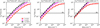 |
Fig. 5 Model 13CO J=1–0 brightness temperatures as a function of H2 column density for volume densities 100, 316, 1000 cm−3, gas kinetic temperatures 10, 30, 100 K, [H2/12CO]=104, and a line width of 11 km s−1. We assume a 12C to 13C abundance ratio of 13.25 (Jacob et al. 2020). The horizontal black line marks the 3σ threshold for the observed peak 13CO brightness temperature from which upper limits on the H2 column density for each model are estimated. |
Column density and X(CO) upper limits from RADEX models for [H2/12CO]=104.
4.3 Virial ratio
The dynamical state of a cloud or clump is evaluated by the virial parameter, αvir, which is the ratio of the virial mass to the luminous mass as derived from spectral line or dust measurements. Clouds with values of αvir < 1 are self-gravitating objects. Assuming the measured velocity dispersion represents random, turbulent motions, clouds with virial ratios between 1 and 2 indicate equipartition between gravitational and kinetic energy densities. If gas motions due to infall significantly contribute to the measured velocity dispersion, then αvir values can vary between 1 and 2 (Ballesteros-Paredes et al. 2011). Measured virial ratios greater than 2 indicate external pressure-bounded clouds or regions that are unbound (Bertoldi & McKee 1992). In practice, the application of the virial ratio to interstellar molecular clouds is challenging as the underlying assumptions and projection effects lead to large uncertainties in αvir values (Beaumont et al. 2013).
From the pycprops segmentation, three clumps (2, 9, 10) are well resolved by the telescope beam, which allows a computation of the virial mass and virial ratio. The pycprops calculation of the virial mass does not include surface terms. The virial mass for clumps 2, 9, and 10 are (2.7±0.3)×104 M⊙, 340±137 M⊙, and 1838±453 M⊙ respectively. The corresponding virial ratio lower limits are 288±32, 68±28, and 157±39. Even with a value of X(CO) 10 times larger in the case of [H2/12CO]=105, the virial ratios would still be greater than 6. These molecular clumps are not bound by self-gravity and are not in equipartition between kinetic and gravitational energy densities.
If the clouds are not bound by external pressure, then the clumps should expand and break up over several clump crossing times, where τcross = 2R/σv. The crossing times for the 3 resolved clumps are 6×10⁵ years (Clump 2), 3×10⁵ years (Clump 9), and 8×10⁵ years (Clump 10), which are ∼3–6 times shorter than the entrainment time of 1.9×10⁶ years estimated from the kinematic, biconical wind model of Di Teodoro et al. (2018). After several crossing time intervals, one would expect the gas to be broadly dispersed and more exposed to the interstellar radiation field leading to a reduced abundance of molecular gas. Yet, the molecular gas persist over these time scales in MW-C21, which argues for stable clumps that are pressure bounded at their surface.
For a non-gravitationally bound system to maintain quasistatic equilibrium, the energy density must be balanced by an external pressure component at the surface. The energy density of a clump, Ucl, is < ρ >  , where < ρ > is the mean mass volume density of the clump and the factor of 3 accounts for a 3 dimensional velocity dispersion. Assuming a spherical clump,
 (4)
(4)
where M is the clump mass. Using the values for Clump 2, the internal energy density is 4.2×10⁻¹⁰ dynes cm−2. For Clumps 9 and 10, the energy densities are 5.5×10⁻¹⁰ and 6.3× 10⁻¹¹ dynes cm−2 respectively.
The molecular clumps are embedded within a cloud of atomic gas with a mass of 428 M⊙ distributed within a radius of 40 pc (Di Teodoro et al. 2018). Assuming a spherical cloud, the mean volume density is 0.06 cm−3. An upper limit on the gas kinetic temperature can be made assuming the measured HI 21 cm velocity dispersion from Di Teodoro et al. (2018) is due to purely thermal motions, such that  /kB =3.5×10⁴ K, where mH is the H I atomic mass and kB is the Boltzmann constant. The upper limit on the cloud thermal pressure, nT, is 2.2×10³ K cm−3 = 4.4×10⁻¹³ dynes cm−2, which is insufficient to bound the internal pressure of the molecular clumps. Cosmic-ray pressure and magnetic field surface tension are possible bounding agents but the strength of each is not well defined in the local environment of MW-C21.
4.4 The role of photodissociation
The molecular gas is exposed to the ambient FUV radiation field that can dissociate H2 molecules. Noon et al. (2023) find evidence for non-equilibrium hydrogen chemistry in MW-C1, MW-C2, MW-C3 in which the molecular gas is photodissociated by the radiation field in the local environment due to insufficient column densities to self-shield H2 molecules. They derive a dissociation time scale,
 (5)
(5)
where χ is the strength of the interstellar radiation field normalized to the Solar neighborhood value. For the 3 resolved clouds, τdiss values are 13/χ Myr (Clump 2), 29/χ Myr (Clump 9), and 6.3/χ Myr (Clump 10). The value of χ in the Fermi Bubble is not well established but would have to be > 10 to be comparable to the entrainment time for MW-C21 in order to have an impact on the amount of molecular gas. MW-C21 is located ∼550 pc above the plane and well displaced from clusters of OB stars so one might expect low χ values (<3) in this environment.
5 Conclusions
We have searched for CO emission from 2 atomic gas clouds associated with the Fermi Bubble. 12CO J=1–0 emission is detected in the cloud MW-C21. This emission is distributed in 11 discrete clumps. 12CO is not detected in the cloud MW-C20 and 13CO J=1–0 emission is not detected in either cloud. Based on RADEX models to predict 13CO J=1–0 brightness temperatures over a range of physical conditions, the absence of detected13 CO emission constrains the H2 column density to be less than 3×1021 cm−2 and the CO to H2 conversion factor, X(CO), to be ≤ 1.6×1020 cm−2 (K km s−1)−1, assuming [H2/12CO]=104. Clump mass upper limits range from 1 M⊙ to 95 M⊙ with a total molecular mass ≤ 132 M⊙, which comprises ≤27% of the neutral gas mass in the cloud. Mass surface density upper limits for the three clumps that are well resolved by the 12″ beam are 18, 42, and 9 M⊙ pc−2. The derived virial ratio lower limits for the three resolved clumps are high (288, 68, 157), yet molecular gas is still present over the entrainment time scale, which suggests that these molecular features are bound by an external pressure component.
Acknowledgements
This work would not have been possible without the longterm financial support from the Mexican Humanities, Science and Technology Funding Agency, CONAHCYT (Consejo Nacional de Humanidades, Ciencias y Tecnologías), and the US National Science Foundation (NSF), as well as the Instituto Nacional de Astrofísica, Óptica y Electrónica (INAOE) and the University of Massachusetts, Amherst (UMass). The operation of the LMT is currently funded by CONAHCYT grant #297324 and NSF grant #2034318. The data described in this paper include LMT observations conducted under the scientific programs, 2023-S1-UM-16 and 2024-S1-MX-2. The LMT welcomes acknowledgement of the scientific and technical support offered by the LMT staff during the observations and generation of data products provided to the authors. This work made use of Astropy (http://www.astropy.org): a community-developed core Python package and an ecosystem of tools and resources for astronomy (Astropy Collaboration 2013, 2018, 2022). LL acknowledges the support of UNAM-DGAPA PAPIIT grants IN108324 and IN112820 and CONACYT-CF grant 263356. E.D.T was supported by the European Research Council (ERC) under grant agreement #10104075. This research was partially funded by the Australian Government through an Australian Research Council Australian Laureate Fellowship (project number FL210100039 awarded to NM-G). The NRAO is a facility of the National Science Foundation operated by Associated Universities, Inc.
References
- Aalto, S., Garcia-Burillo, S., Muller, S., et al. 2012, A&A, 537, A44 [NASA ADS] [CrossRef] [EDP Sciences] [Google Scholar]
- Astropy Collaboration (Robitaille, T. P., et al.) 2013, A&A, 558, A33 [NASA ADS] [CrossRef] [EDP Sciences] [Google Scholar]
- Astropy Collaboration (Price-Whelan, A. M., et al.) 2018, AJ, 156, 123 [Google Scholar]
- Astropy Collaboration (Price-Whelan, A. M., et al.) 2022, ApJ, 935, 167 [NASA ADS] [CrossRef] [Google Scholar]
- Ballesteros-Paredes, J., Hartmann, L. W., Vázquez-Semadeni, E., Heitsch, F., & Zamora-Avilés, M. A. 2011, MNRAS, 411, 65 [NASA ADS] [CrossRef] [Google Scholar]
- Beaumont, C. N., Offner, S. S. R., Shetty, R., Glover, S. C. O., & Goodman, A. A. 2013, ApJ, 777, 173 [NASA ADS] [CrossRef] [Google Scholar]
- Bertoldi, F., & McKee, C. F. 1992, ApJ, 395, 140 [NASA ADS] [CrossRef] [Google Scholar]
- Bolatto, A. D., Wolfire, M., & Leroy, A. K. 2013, ARA&A, 51, 207 [CrossRef] [Google Scholar]
- Di Teodoro, E. M., McClure-Griffiths, N. M., Lockman, F. J., et al. 2018, ApJ, 855, 33 [Google Scholar]
- Di Teodoro, E. M., McClure-Griffiths, N. M., Lockman, F. J., & Armillotta, L. 2020, Nature, 584, 364 [NASA ADS] [CrossRef] [Google Scholar]
- Efron, B. 1979, Ann. Statist., 7, 1 [Google Scholar]
- Heywood, I., Camilo, F., Cotton, W. D., et al. 2019, Nature, 573, 235 [Google Scholar]
- Jacob, A. M., Menten, K. M., Wiesemeyer, H., et al. 2020, A&A, 640, A125 [EDP Sciences] [Google Scholar]
- Krumholz, M. R. 2014, MNRAS, 437, 1662 [NASA ADS] [CrossRef] [Google Scholar]
- Lewis, J. A., Lada, C. J., & Dame, T. M. 2022, ApJ, 931, 9 [NASA ADS] [CrossRef] [Google Scholar]
- McClure-Griffiths, N. M., Green, J. A., Hill, A. S., et al. 2013, ApJ, 770, L4 [Google Scholar]
- Nakashima, S., Koyama, K., Wang, Q. D., & Enokiya, R. 2019, ApJ, 875, 32 [NASA ADS] [CrossRef] [Google Scholar]
- Narayanan, G., Heyer, M. H., Brunt, C., et al. 2008, ApJS, 177, 341 [NASA ADS] [CrossRef] [Google Scholar]
- Noon, K. A., Krumholz, M. R., Di Teodoro, E. M., et al. 2023, MNRAS, 524, 1258 [NASA ADS] [CrossRef] [Google Scholar]
- Oka, T., Hasegawa, T., Sato, F., et al. 2001, ApJ, 562, 348 [Google Scholar]
- Ponti, G., Hofmann, F., Churazov, E., et al. 2019, Nature, 567, 347 [Google Scholar]
- Putman, M. E., de Heij, V., Staveley-Smith, L., et al. 2002, AJ, 123, 873 [NASA ADS] [CrossRef] [Google Scholar]
- Rosolowsky, E., & Leroy, A. 2006, PASP, 118, 590 [NASA ADS] [CrossRef] [Google Scholar]
- Silk, J., & Mamon, G. A. 2012, Res. Astron. Astrophys., 12, 917 [Google Scholar]
- Su, M., Slatyer, T. R., & Finkbeiner, D. P. 2010, ApJ, 724, 1044 [Google Scholar]
- Teuben, P., Heyer, M., Mundy, L., et al. 2024, in Astronomical Society of the Pacific Conference Series, 535, eds. B. V. Hugo, R. Van Rooyen, & O. M. Smirnov, 149 [NASA ADS] [Google Scholar]
- Thompson, T. A., Quataert, E., Zhang, D., & Weinberg, D. H. 2016, MNRAS, 455, 1830 [CrossRef] [Google Scholar]
- van der Tak, F. F. S., Black, J. H., Schöier, F. L., Jansen, D. J., & van Dishoeck, E. F. 2007, A&A, 468, 627 [NASA ADS] [CrossRef] [EDP Sciences] [Google Scholar]
- Veilleux, S., Maiolino, R., Bolatto, A. D., & Aalto, S. 2020, A&A Rev., 28, 2 [NASA ADS] [CrossRef] [Google Scholar]
- Walter, F., Bolatto, A. D., Leroy, A. K., et al. 2017, ApJ, 835, 265 [NASA ADS] [CrossRef] [Google Scholar]
All Tables
All Figures
|
Fig. 1 Images of atomic hydrogen column density, 12CO and 13CO integrated intensities for (top row) MW-C20 and (bottom row) MW-C21. The N(H I) contour levels are (0.5, 1, 1.5)×1019 cm−2 and (1, 2, 3, 4)×1019 cm−2, respectively. While 12CO emission is visible in several regions of MW-C21, the broad velocity range with respect to the narrow velocity components dilutes the signal with excess noise. No 13CO J=1−0 emission is detected in either cloud. The red circles show the GBT half power beam width of the HI observations. The red circles in the lower right corner of the middle and right images denote the half power beam widths at 12CO and 13CO. |
| In the text | |
|
Fig. 2 Image of 12CO integrated intensities of clumps in MW-C21 based on the 3 dimensional mask array that identifies islands of connected CO emission. The dotted contours show the distribution of atomic hydrogen column density with contour levels (1, 2, 3, 4)× 1019 cm−2. |
| In the text | |
|
Fig. 3 Coadded average 12CO J=1−0 spectra for each molecular clump in MW-C21 based on the 3 dimensional mask array. |
| In the text | |
|
Fig. 4 Images of 12CO (left) integrated intensities and (right) centroid velocities that combine the masks for Clump 1 and Clump 2. The contours show the distribution of 12CO integrated intensities with levels 1, 3, 5, 7, 9 K km s−1. |
| In the text | |
|
Fig. 5 Model 13CO J=1–0 brightness temperatures as a function of H2 column density for volume densities 100, 316, 1000 cm−3, gas kinetic temperatures 10, 30, 100 K, [H2/12CO]=104, and a line width of 11 km s−1. We assume a 12C to 13C abundance ratio of 13.25 (Jacob et al. 2020). The horizontal black line marks the 3σ threshold for the observed peak 13CO brightness temperature from which upper limits on the H2 column density for each model are estimated. |
| In the text | |
Current usage metrics show cumulative count of Article Views (full-text article views including HTML views, PDF and ePub downloads, according to the available data) and Abstracts Views on Vision4Press platform.
Data correspond to usage on the plateform after 2015. The current usage metrics is available 48-96 hours after online publication and is updated daily on week days.
Initial download of the metrics may take a while.