


| Issue |
A&A
Volume 711, July 2026
|
|
|---|---|---|
| Article Number | A291 | |
| Number of page(s) | 17 | |
| Section | Extragalactic astronomy | |
| DOI | https://doi.org/10.1051/0004-6361/202558758 | |
| Published online | 22 July 2026 | |
Dynamical models of cluster members to probe the total mass properties of cluster subhalos
I. A comparison with parametric strong lensing models
1
Dipartimento di Fisica, Università degli Studi di Milano, Via Celoria 16, I-20133 Milano, Italy
2
INAF – IASF Milano, Via Corti 12, I-20133 Milano, Italy
3
Dipartimento di Fisica e Scienze della Terra, Università degli Studi di Ferrara, Via Saragat 1, I-44122 Ferrara, Italy
4
Institute of Cosmology and Gravitation, University of Portsmouth, Burnaby Rd, Portsmouth PO1 3FX, UK
5
INAF – Osservatorio di Astrofisica e Scienza dello Spazio di Bologna, Via Piero Gobetti 93/3, I-40129 Bologna, Italy
6
Università di Salerno, Dipartimento di Fisica “E.R. Caianiello”, Via Giovanni Paolo II 132, I-84084 Fisciano (SA), Italy
7
INAF – Osservatorio Astronomico di Capodimonte, Via Moiariello 16, I-80131 Napoli, Italy
8
INFN – Gruppo Collegato di Salerno – Sezione di Napoli, Dipartimento di Fisica “E.R. Caianiello”, Università di Salerno, Via Giovanni Paolo II, 132, I-84084 Fisciano (SA), Italy
9
Independent researcher, Ismaning 85737, Germany
★ Corresponding author: This email address is being protected from spambots. You need JavaScript enabled to view it.
Received:
23
December
2025
Accepted:
1
June
2026
Abstract
In this series of papers, we present dynamical models of cluster members in strong lensing galaxy clusters to independently probe the persistent discrepancy reported between strong lensing models and cosmological hydrodynamical simulations, in terms of total mass properties for the cluster subhalos. In this work, we focused our study on early-type galaxies within the clusters Abell 2744 (z = 0.309) and MACS J0416.1−2403 (z = 0.397). We took advantage of deep spectroscopic data from the Multi Unit Spectroscopic Explorer (MUSE), on the Very Large Telescope, complemented with Hubble Frontier Fields photometry. We used a pipeline based on spectral fitting to perform kinematic measurements of the line-of-sight velocity dispersion profiles of 109 cluster members, extending, in the best cases, up to approximately 15 kpc from the galactic centers. We modeled the cluster members assuming a dual pseudo-isothermal total mass density distribution and a Jaffe stellar mass density distribution. From the models, we inferred the values of the central stellar velocity dispersion, σ0, and the truncation radius, rt, for the galaxies in our sample. We found that σ0 is accurately recovered for all of the cluster members and varies approximately from 40 km s−1 to 370 km s−1, while rt is reliably measured for a fraction of galaxies in our sample, with sufficiently extended radial kinematic coverage. Our dynamical models predicted line-of-sight velocity dispersion profiles that fit the measured ones better than those inferred from strong lensing models. To tackle the discrepancy from the strong lensing side, we exploited the σ0 measurements obtained from the dynamical models to calibrate the Faber-Jackson scaling relations for the cluster members in both galaxy clusters. When comparing our relations to those obtained in previous kinematics and strong lensing works, we found systematically higher normalization and compatible slope and scatter values. We conclude that our dynamical measurements of σ0 and rt, along with calibrated scaling relations, are more robust than previous kinematic estimates (which are biased due to not taking into account the effects of the point spread function and of averaging inside the aperture) and should therefore be adopted as improved initial prescriptions in future strong lensing models.
Key words: gravitational lensing: strong / galaxies: clusters: individual: MACS J0416.1-2403 / galaxies: clusters: individual: Abell 2744 / galaxies: kinematics and dynamics / galaxies: structure / dark matter
© The Authors 2026
 Open Access article, published by EDP Sciences, under the terms of the Creative Commons Attribution License (https://creativecommons.org/licenses/by/4.0), which permits unrestricted use, distribution, and reproduction in any medium, provided the original work is properly cited.
This article is published in open access under the Subscribe to Open model. This email address is being protected from spambots. You need JavaScript enabled to view it. to support open access publication.
1. Introduction
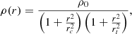
The Λ cold dark matter (ΛCDM) cosmological model describes the Universe with CDM particles that interact only through gravity, and a cosmological constant, Λ. From this cosmological paradigm, we know that large-scale structures in our Universe formed hierarchically, by mergers of smaller halos (Tormen 1997; Moore et al. 1999). This process led to the formation of clusters of galaxies. Dark matter (DM) constitutes ∼85 − 90% of the total mass of clusters (Zwicky 1933; Fabricant et al. 1986; Eyles et al. 1991; Smail et al. 1995; Kneib et al. 1996; Medezinski et al. 2010; Grillo et al. 2015). This component is further subdivided into cluster-scale DM halos and galaxy-scale DM subhalos. The remaining 10 − 15% of the mass budget is made up of baryons. Galaxy clusters contain thousands of galaxies embedded in the DM subhalos (Bertin & Stiavelli 1993; Bacon et al. 2001; Gerhard et al. 2001) and are thus ideal astrophysical laboratories for studying the physical properties of DM and its interactions with baryons, together with the formation and evolution of galaxies. Two different methods of studying the mass distribution of clusters and their member galaxies are cosmological hydrodynamical simulations and strong gravitational lensing (SL from here on). Starting from some initial prescriptions about the nature of DM and its interplay with baryons, and about feedback processes, cosmological simulations follow the growth of portions of the Universe. From these simulated boxes of the Universe, one can extract information about DM halos and subhalos. Simulations show that DM halos of any mass have approximately self-similar mass density profiles, with a central cusp, usually described using the Navarro-Frenk-White (NFW; Navarro et al. 1997) or Einasto (Einasto 1965) distributions. Any significant discrepancy between the predictions of simulations and observations may imply that the formation of structures does not proceed as predicted by the ΛCDM model, or that some of the initial prescriptions in the simulations are inaccurate or incomplete. Strong lensing models measure the mass properties of DM halos by reconstructing the positions of multiple images of lensed sources that lie behind an observed massive object, such as a galaxy cluster. Strong lensing is particularly effective in cluster cores, where multiple images of background sources are typically observed. However, some degeneracies critically limit the accuracy of SL in reconstructing the mass structure of galaxy cluster subhalos (Meneghetti et al. 2017; Bergamini et al. 2019). These degeneracies stem from the fact that SL is sensitive to the total mass distribution on scales typically larger than those of a single cluster galaxy, and they can be broken by exploiting independent measurements of the stellar velocity dispersion of cluster members (Falco et al. 1985; Treu & Koopmans 2004; Meylan et al. 2006; Barnabè et al. 2009). In state-of-the-art parametric SL models, cluster members are typically modeled with the spherical version of the dual pseudo-isothermal elliptical (dPIE) total mass density distribution (Grillo et al. 2015). The spherical version of a dPIE resembles a singular isothermal sphere (SIS), but it presents a core radius, rc, and a truncation radius, rt, which define the radial scales of the transition from a cored, ρ ∝ r0, to an isothermal, ρ ∝ r−2, to a ρ ∝ r−4 profile. The dPIE mass density profile is defined as
 (1)
(1)
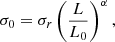
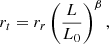
where  and σ0 is the central velocity dispersion value. After assuming a vanishing rc, the SL models are left with two free parameters for each cluster member: σ0 and rt. To reduce the number of free parameters, the most recent parametric SL models include power-law scaling relations for the velocity dispersion and the truncation radius of the cluster members. Moreover, state-of-the-art SL models include kinematic priors on cluster galaxies to break the aforementioned degeneracies and calibrate the scaling relations with respect to the total luminosity, L, of each member:
 (2)
(2)
 (3)
(3)
where σr and rr are optimized reference values for σ0 and rt, of the member galaxies, and L0 is a luminosity reference value. The first equation, the Faber-Jackson (F-J; Faber & Jackson 1976) scaling relation, is calibrated with kinematic data points, while the slope of the second relation is connected to the slope of the first through the fundamental plane (FP; Djorgovski & Davis 1987), as γ = 2α + β − 1, where γ is connected to the tilt of the FP. Alternatively, SL models can utilize the FP, a more accurate and complex relation, to directly link the velocity dispersion of the members to their structural parameters (Granata et al. 2022). In this work, we intend σ0 as defined in the dPIE total mass density distribution. This velocity dispersion value is not to be confused with the σ0 adopted in the FP relation, which is defined as the galaxy stellar velocity dispersion through an aperture of radius r = Re/8, with Re being the effective radius.
As found by Meneghetti et al. (2020), cosmological hydrodynamical simulations underestimate the number of galaxy-galaxy SL events. An interpretation proposed to explain the lack of these events in simulations requires that these underpredict the number of massive and compact substructures inside clusters of galaxies (Meneghetti et al. 2022, 2023).
In order to investigate the origin of this discrepancy, in this series of works, we built dynamical models of elliptical cluster members in SL galaxy clusters (Binney 1982; Binney & Mamon 1982; Binney & Tremaine 2011) to test SL models and cosmological simulation claims. This is ideal, since dynamics gives a completely independent probe of the total mass distribution of these objects.
Several Hubble Space Telescope (HST) programs provide deep observations of SL events in the cores of massive clusters, such as the Cluster Lensing And Supernova survey with Hubble (CLASH; Postman et al. 2012), the Hubble Frontier Fields (HFF; Lotz et al. 2017) campaign, and the Reionization Lensing Cluster Survey (RELICS; Coe et al. 2019). As a follow-up, spectroscopic campaigns, such as CLASH-VLT (Rosati et al. 2014), or spectroscopic measurements from the integral field Multi Unit Spectroscopic Explorer (MUSE; Bacon et al. 2010) on the Very Large Telescope (VLT), have permitted secure identifications of cluster members and precise redshift measurements for hundreds of multiply lensed sources. These data enable the construction of SL models, such as those presented in Bergamini et al. (2023a,b, hereafter B+23a and B+23b), and the development of detailed dynamical models of cluster members. MUSE deep spectroscopic observations can be used to measure the line-of-sight (LOS) velocity dispersion profiles for the cluster members. The values of the kinematics of cluster members obtained with dynamical models can then be used to calibrate the F-J scaling relations and compare them with those used in SL models, consequently probing the reliability of their conclusions. In this first paper, we focus on the description of the Jeans dynamical models for the cluster members in our dataset. We then discuss the possibility of measuring key total mass quantities that can immediately be used to better calibrate the scaling relations adopted as priors in SL models. Improving the SL models represents a first step toward the resolution of the discrepancy.
The paper is organized as follows. In Sect. 2, we provide details on our photometric and spectroscopic data. In Sect. 3, we describe the assumptions adopted to build the dynamical models for elliptical cluster members and the main parameters that can be inferred. In Sect. 4, we discuss the results of the inference procedure performed using the dynamical models. We then present a comparison between the prediction of dynamical and SL models on the LOS velocity dispersion profiles and on the F-J scaling relations. In Sect. 5, we summarize our key findings and discuss some future prospects. In this work, we assume a flat ΛCDM cosmological model with H0 = 70 km s−1 Mpc−1 and Ωm = 0.30.
2. Data
In this section we summarize the photometric and spectroscopic datasets for the two clusters of galaxies studied in this work, namely Abell 2744 and MACS J0416.1−2403, hereafter A2744 and M0416, at redshifts z = 0.309 (Allen 1998; Ebeling et al. 2010) and z = 0.397 (Balestra et al. 2016), respectively. Abell 2744 was first discovered in Couch & Newell (1984), with a measured virial mass of M = 4.0 × 10¹⁵ M⊙ (Merten et al. 2011), while M0416 was first discovered during the MAssive Cluster Survey (MACS; Ebeling et al. 2001), with a measured virial mass of M = 0.9 × 10¹⁵ M⊙ (Balestra et al. 2016). Both A2744 and M0416 were further studied during the HFF programme (Lotz et al. 2017). The HFF observed a restricted sample of clusters, for 140 orbits each, providing deep imaging in seven different bands (HST/ACS F435W, F606W, and F814W; and HST/WFC3 F105W, F125W, F140W, and F160W). M0416 was also included in the CLASH-VLT survey (P.I.: P. Rosati) to obtain spectroscopic data to complement HST imaging (Postman et al. 2012). The magnitudes and effective radii in the F814W and F160W bands for A2744 and M0416 were measured, together with all other structural parameters, in Granata et al. (2026) and Tortorelli et al. (2023), respectively, using the Python package MORPHOFIT (Tortorelli & Mercurio 2023), based on SExtractor (Bertin & Arnouts 1996) and Galfit (Peng 2010).
Spectroscopic information from the core of each cluster was obtained with the MUSE instrument, covering a spectral range between 4800 Å and 9300 Å and with a spectral resolution between R ≈ 1750 at 4650 Å and R ≈ 3750 at 9300 Å, and a spectral sampling of 1.25 Å/pixel. The data analyzed in this paper were obtained in wide-field mode (WFM), with a field of view of 1′×1′, and a pixel size of 0.2″ × 0.2″. In detail, for M0416, the NE and SW regions of the core were observed with MUSE for 17.1 h (Vanzella et al. 2021) and 11 h (Caminha et al. 2017), respectively, while for A2744 the core was observed with five different MUSE pointings, with total exposure times of between 2 − 5 h (Mahler et al. 2018; Richard et al. 2021). Moreover, adaptive optics (AO) was utilized in 14 of the 18 exposures in the NE region of M0416 (Vanzella et al. 2021). The effects of AO on the spectral cubes were taken into account during the MUSE data reduction procedure. The MUSE data analyzed in our work have recently been used in Mozumdar et al. (2025a,b) to study the structure, kinematics, and stellar populations of some cluster members.
3. Methods
This section briefly describes how we built the dynamical models of the cluster members, using their measured LOS velocity dispersion profiles and starting from some assumptions about the galaxy symmetry, the total and stellar mass distributions, and the anisotropy of the stellar orbits. The equation for the LOS velocity dispersion profiles, along with the procedure that allows us to account for aperture and point-spread-function (PSF) effects, is discussed in detail in Appendix A. We also outline here the selection criteria we followed to define the cluster member sample, as well as all the methods employed to perform the kinematic measurements on each galaxy. Here, we assume that the stellar mass density distribution of galaxies follows the stellar luminosity density distribution, meaning that the light emitted by the stars also traces how their mass is distributed within a galaxy (the mass-follows-light assumption from here on).
3.1. Total and stellar mass profiles
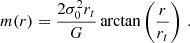
As is discussed in Appendix A, in order to model the LOS velocity dispersion profile of a galaxy using Eq. (A.2), one needs to assume a total and a stellar mass distribution. Elliptical galaxies are often modeled with a dPIE total mass density profile (see Eq. (1)). This density profile can be integrated to obtain the total mass of the galaxy within a sphere of radius r. Assuming a vanishing central core for the analyzed galaxies, rc = 0, we then obtain
 (4)
(4)
The choice of a dPIE profile for the total mass density profile of cluster members is justified, for instance, by the results obtained by Grillo et al. (2015), where modeling cluster members with such a total mass density distribution is shown to lead to parametric SL models that reproduce the observed positions of multiple images well. Finally, to build dynamical models, we need to make some assumptions about the stellar mass density distribution. The Jaffe profile (Jaffe 1983) is often used for this purpose. Under the mass-follows-light assumption, it is possible to substitute the total mass of the stars inside an elliptical galaxy, M, with their total luminosity, L, to obtain
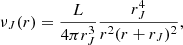 (5)
(5)
where rJ is a scale radius, related to the effective radius as rJ = Re/0.763. Equation (5) allows for the determination of the surface brightness profile of an elliptical galaxy, to be substituted into Eq. (A.3), thereby providing a dynamical model of the galaxy.
In the paper, we primarily focus on the dynamical results obtained assuming dPIE and Jaffe profiles for the total and stellar mass density profiles, respectively (hereafter referred to as the dPIE-J model). To properly test the model systematics and strengthen our conclusions, in Appendix B we also present the results obtained by exploiting a NFW total mass density distribution and a Hernquist luminosity density distribution. The additional dynamical models are referred to as NFW-Jaffe (hereafter NFW-J) and dPIE-Hernquist (hereafter dPIE-H), respectively.
3.2. The kinematic measurements
In this section we describe the pipeline we exploited to perform the kinematic measurements on the cluster members. We then discuss the measurement details and selection procedure that was followed to obtain the measured LOS velocity dispersion profiles.
3.2.1. The pPXF algorithm
To perform the kinematic measurements on cluster members, we adopted the penalized pixel fitting (pPXF) software by Cappellari & Emsellem (2004). In our case, pPXF measures the first two line-of-sight-velocity-distribution (LOSVD) parameters by comparing the galaxy observed spectra with a set of 463 stellar templates we took from the second data release (DR2) of the X-shooter Spectral Library (Gonneau et al. 2020), convolved with a LOSVD. In addition, the algorithm utilizes additive polynomials to compensate for potential template mismatches, adjust the intensity of spectral lines, account for inaccurate spectral calibrations and dust reddening, and mitigate sky contributions to the spectrum. The LOSVD was obtained after assuming a Gaussian parametrisation, where we only fit the first two moments of the distribution, namely the peculiar velocity and velocity dispersion values. The set of moments of the LOSVD were obtained by the algorithm through an optimization procedure, performed to minimize the differences between the observed and the synthetic galaxy spectra, exploiting a standard χ2 function. The first two moments of the LOSVD were thus measured, along with their corresponding uncertainties, and an average signal-to-noise value, ⟨S/N⟩, was used to evaluate the reliability of the kinematic measurements. We tested that unreliable values for the kinematic parameters were obtained when S/N < 10. For S/N ≥ 10, the optimized values can still present a bias in the cases of spectral contamination or inaccurate fit (Cappellari & Emsellem 2004). In this work, the fits were performed on a rest-frame wavelength range of [3700, 5100] Å. Further details about the kinematic pipeline we adopted are discussed in Granata et al. (2026). An example of the output of the fitting procedure is shown in Fig. 1. The figure presents both the observed (in black) and fit (in red) spectra, the residuals (green dots), and the optimized LOSVD first two moments values for a cluster member in M0416. From the figure, it can be seen that the most important absorption lines used to fit the spectra in the available spectral range are the CaII K/H lines and the G band, at 3934 Å, 3969 Å and 4310 Å (rest-frame), respectively. Galaxy emission lines, sky lines, and telluric lines have been masked (grey bands in the Figure), as in Bergamini et al. (2019, hereafter B+19). As mentioned in Sect. 2, the effects of AO were properly accounted for during the reduction procedure of the MUSE observations in M0416 NE. Consequently, we decided not to mask the wavelength region in which possible AO residuals lie, namely [5800, 6000] Å observed-frame. We checked that masking this interval does not influence our conclusions and that the differences that arise in the kinematic measurements with and without the mask are minor and lie below other small systematic effects that we did not consider in this work. From the figure, it is also possible to note how the depth of the MUSE observations in the cluster cores yields detailed galaxy spectra, which remarkably display a large number of characteristic absorption lines. This significantly impacts the S/N value obtained from the pPXF fitting procedure and the reliability of the measured values of the kinematic quantities and their associated errors (Granata et al. 2026).
 |
Fig. 1. Spectrum of the cluster galaxy 80726 in M0416, extracted from a circular aperture with radius r = 0.5″ centered on the galaxy luminosity center. The black line shows the measured spectrum, while the red line shows the fit spectrum, obtained with the pPXF pipeline, from rest-frame 3700–5100 Å. On the bottom, the residuals between the two spectra are shown as green dots. The gray bands highlight masked regions. On the top, the values of the extracted kinematic parameters are listed: the velocity dispersion, σ, and the peculiar velocity, v, in kilometers per second, with their corresponding uncertainties, and the average signal-to-noise ratio ⟨S/N⟩. |
3.2.2. The galaxy sample selection procedure
The first step in measuring the LOS velocity dispersion profiles is the selection of a sample of elliptical galaxies within each of the two studied clusters. Starting from the full cluster member catalogs for both A2744 and M0416 (B+23a; B+23b)1, we required each selected galaxy to be isolated, meaning that there are no other objects closer than 1.5″ in projection. This selection procedure was performed since some contamination from another neighboring galaxy could modify the morphology and the measured spectrum of the galaxy, substantially impacting the measured values of the kinematic parameters. Moreover, a galaxy that is surrounded by other galaxies could be influenced in its dynamics by tidal interactions. These interactions could lead to LOS velocity dispersion profiles that are much more complicated than those intended to be studied in this work. We then required each selected galaxy to have a S/N > 30 when a pPXF fit was performed within a circular aperture of 0.8″, centered on its center. Since we want to infer the galaxy truncation radius, we aim to construct LOS velocity dispersion profiles with radial extensions exceeding 1″. The requirement on the S/N thus favors measured profiles with at least two data points. We can still infer the σ0 values of the few galaxies with one single measurement. Following these preliminary criteria, lists of 89 and 87 members for M0416 and A2744, respectively, were obtained for further analysis.
3.2.3. The kinematic LOS velocity dispersion profiles
For each of the 176 preliminary selected galaxies, we then performed a pPXF fit inside annuli of 0.5″ fixed width and of increasing radial size, to measure their LOS velocity dispersion profiles. An example of this annular subdivision is shown in Fig. 2. The minimum width was fixed to be of the same order as the observation PSF. A measured LOS velocity dispersion profile for a M0416 cluster member is shown in Fig. 3. In the figure, the uncertainties on σLOS are extracted from the pPXF algorithm, while each annulus width is chosen as the uncertainty on the radius. The progressive increase in the σLOS uncertainties with the radial distance from the galactic center is due to lower S/N values in the outer regions of a galaxy, as a consequence of lower surface brightness. After the measured LOS velocity dispersion profiles were built, a further selection procedure was pursued. Exploiting HFF RGB images and MUSE spectra, it is possible to discard the profiles of those galaxies disturbed by external objects, such as foreground or background galaxies and lensed objects, or by starburst processes. Such interference can be recognized by carefully analyzing the extracted spectra for each galaxy within each annulus, searching for abrupt changes in the residuals between nearby annuli and for emission lines that are typically not expected in an elliptical galaxy spectrum.
 |
Fig. 2. MUSE cube cutout of the galaxy 80726 in the cluster of galaxies M0416. The annuli of 0.5″ width and increasing radial size, within which the LOS velocity dispersion profile was measured, are shown. |
 |
Fig. 3. Measured LOS velocity dispersion profile of galaxy 80726 as a function of the radial distance from the center, in both arcseconds (bottom) and kiloparsecs (top). The red lines along the horizontal axis show the uncertainty on the measurement position due to each annulus width, as shown in Fig. 2, while the ones along the vertical axis represent the uncertainty on each measured σLOS, obtained from the pPXF pipeline. |
As discussed above, pPXF is able to reliably measure the kinematic parameters and the relative uncertainties for a galaxy only if the spectrum S/N > 10. To make sure that the pPXF uncertainties are unbiased (Granata et al. 2026) we required each of the LOS velocity dispersion measurements to have a S/N > 10. Moreover, we demanded S/N > 30 in order to proceed with the kinematic measurement in the successive annulus (e.g., in a five-point LOS velocity dispersion profile, the first four points satisfy S/N ≥ 30 while the last one has 10 ≤ S/N < 30). These quite stringent limits could be relaxed in future works to allow for an extension of the sample of cluster members. Following this procedure, we obtained a total of 109 LOS velocity dispersion profiles. Within this sample, 17 profiles have three or more measured points. We highlight once again that the number of points in each LOS velocity dispersion profile is fundamental in order to reliably extract information about the truncation of the aforementioned total mass profiles. A kinematic profile that only has one or two σ measurements is typically not extended enough radially to properly investigate its truncation. On the other hand, the central stellar velocity dispersion is reliably measured, independently of the radial extension of the LOS velocity dispersion profile, as is discussed later in the paper.
Finally, from the assumptions on elliptical galaxies total and stellar mass density distributions, we made in Sect. 3.1, we expect their LOS velocity dispersion profiles to decrease with r. Nonetheless, in our measurements we observe a fraction of increasing profiles. Such an increase could be a symptom of tidal interactions with other cluster members or a significant rotation of the galaxy. From the combination of photometric and spectroscopic analysis, it is possible to conclude that some objects classified as elliptical galaxies in the cluster member catalogs are actually either lenticular galaxies or fast rotators (Cappellari & Emsellem 2004). A rotational contribution to the LOS velocity dispersion profile is considered to be a velocity dispersion by pPXF, because kinematic measurements performed through annular apertures lead to a superposition of the red and blue shift in the galaxy spectral lines, caused by the ordered motion of the stars inside the galaxy that are, respectively, moving away and toward the observer. To disentangle the overlapping σ − vrot contributions, one could choose a rotation axis for these fast rotating galaxies and perform separated kinematic measurements within semi-annuli centered on that axis. To enlarge the sample of galaxies, future analyses will take this effect into account.
3.3. Jeans dynamical models of cluster members
As is discussed in Appendix A and Sect. 3.1, by substituting Eq. (4) as the total mass density distributions and Eq. (5) as the stellar luminosity density distribution in Eq. (A.2), one obtains a Jeans dynamical model for the LOS velocity dispersion profile. Exploiting HFF photometric data (see Sect. 2), one can compute the luminosity for each of the galaxies in our sample, starting from their F814W magnitude. The scale radius, rJ, is related to Re and is thus immediately obtained. It is then possible to combine the kinematic measurements and the dynamical model for the LOS velocity dispersion profiles to infer the values of σ0 and rt. To perform the inference procedure, we exploited the Markov chain Monte Carlo (MCMC) optimization algorithm emcee (Foreman-Mackey et al. 2013). We defined wide flat prior distributions for the two free parameters: σ0 ∈ [10, 1000] km s−1 and rt ∈ [0.01, 200] kpc. For each of the sample galaxies, we randomly selected a starting value for the free parameters within such priors. We then performed the MCMC optimization using chains with 4 walkers and 15 000 steps each. Considering the autocorrelation time, we discarded the first 1000 steps for each chain. We obtained as outputs the corner plots and posterior probability distributions for the free parameters. An example of the corner plots for a galaxy in M0416, parametrized with the dPIE-J dynamical model, is shown in Fig. 4. From the obtained posterior probability distributions, one can use the dynamical models to compute the predicted LOS velocity dispersion profiles and compare them with the kinematic measurements, as shown in Fig. 5. From the figure, which compares 100 profiles obtained from the dPIE-J dynamical models (in orange) of a M0416 cluster member (ID: 83064) with the kinematic measurements (in black), it is clear that the model is good at reproducing the measured profiles.
 |
Fig. 4. Corner plot obtained from the inference procedure on the cluster galaxy 83064 in M0416. The posterior probability distributions for σ0 and rt and their correlation are shown. The median values and 16th and 84th percentiles are reported at the top and highlighted with blue and green lines. |
 |
Fig. 5. Comparison between measured and model-predicted velocity dispersion profiles. In black, we show the profile obtained from the kinematic measurements (red data points) of the cluster member 83 064 in M0416. As solid orange lines, we plot 100 profiles obtained with the dynamical model by sampling the posterior distributions of the free parameters, drawn from the MCMC optimization and shown in Fig. 4. The distance from the galactic center is reported in arcseconds (bottom) and kiloparsecs (top). |
In the following, we focus on how the values of σ0 inferred from the modeling can be used for calibrating a F-J scaling relation on the sample galaxies for both A2744 and M0416. We highlight that this procedure is substantially different from aperture measurements of the stellar velocity dispersion, such as the ones performed in B+23a and Bergamini et al. (2021, hereafter B+21). The first difference is due to the fact that we measure the actual central value, σ0, whereas a measurement through an aperture yields a mean σ value within the aperture. This effect can be seen in Fig. 5, where the σ value measured in the first annulus (in black) is clearly lower than the central value obtained from the dynamical model (in orange). More importantly, the values measured within the apertures in B+23a and B+21 typically do not take into account the PSF of the observations, which, when convolved with the σLOS, dims the central values of the profile. These effects on the measured galaxy kinematics and, subsequently, on the calibration of the F-J scaling relation are discussed in depth in the next section.
4. Results and discussion
In this section we discuss the main results obtained through dynamical modeling and compare them with the state-of-the-art parametric SL models (B+23a; B+23b) and stellar kinematic measurements (B+23a; B+21). The comparison between the predictions of the different model parametrizations is presented in Appendix B.
4.1. The different truncation radius classes
Following the procedures outlined in the previous section, we were able to obtain information about σ0 and rt for all of the 109 selected galaxies. The measured photometric properties and the inferred values of the model parameters are listed in Tables D.1 and D.2 for galaxies with, respectively, at least and fewer than three measured kinematic points. For all the galaxies in our sample, we obtained a posterior distribution of σ0 similar to a Gaussian distribution. We then divided the sample of galaxies into three different classes: “Gaussian”, “tailed”, and “flat”, depending on the shape of the inferred rt posterior distribution. For 97 galaxies, we obtained a flat posterior distribution for rt (see Fig. 6, left corner plot); for 5 we obtained a tailed posterior distribution (see Fig. 6 right corner plot); and for 7 we obtained a simil-Gaussian distribution (see Fig. 4). The rt median values obtained for the flat galaxies depend on the selected prior, rendering the truncation estimates for flat galaxies unusable. The inability of the dPIE models to consistently obtain a reliable value for the truncation radius of a galaxy can be justified as follows:
-
Since all of the galaxies that have measured kinematic profiles with fewer than three points are classified as flat (except for one, ID: 81285), we can conclude that for these galaxies the truncation radius probably lies outside of the range covered by our kinematic measurements.
-
We noticed that the six galaxies with more than two measured kinematic points, classified as flat, exhibit a rotational velocity contribution that increases with radial distance from their center. This leads to higher measured σap values on the outskirts of the galaxies, subsequently causing a flattening of the measured profiles. We thus suggest that more complex dynamical models that take into account both the stellar velocity dispersion and rotation are needed to reliably measure the rt values for these galaxies. Nonetheless, the lack of strong rotation in the inner regions of these galaxies (e.g., Zhu et al. 2023) allows us to conclude that the σ0 measurements of these cluster members are reliable.
-
For the five galaxies classified as tailed, the rotation effect described above is present but does not strongly influence the measured profiles. To test this, we performed the inference procedure on some of the galaxies classified as Gaussian, removing the last LOS velocity dispersion measurement. It appears that having a rt that is on the edge of the kinematic measurements does impact the recovered rt posterior distribution, resulting in a tail. However, this does not influence significantly the estimated σ0 values. This suggests once again that the lack of radially extended kinematic measurements prevents us from precisely evaluating the truncation radius of some galaxies.
 |
Fig. 6. Corner plots of the central stellar velocity dispersion, σ0, and truncation radius, rt, for two cluster members (38 729 on the left and 34 423 on the right) in A2744, obtained from the inference procedure. The posterior probability distributions of σ0 and rt and their correlations are shown. The median values and percentiles are highlighted as in Fig. 4. The rt posterior probability distributions for these galaxies are classified as flat and tailed, respectively. The σ0 posterior distribution is close to a Gaussian distribution for both galaxies. |
Thus, for all 109 sample galaxies, the σ0 values are reliably inferred, while rt is measured for only 12 cluster members. Given the fact that we can reliably recover the values of rt only for a fraction of the sample of cluster members, no statistically significant conclusions about the compactness of these objects and its effects on the discrepancy between SL models and cosmological simulations can be made. We refer the reader to the next paper of this series in which we shall increase the statistics of our analysis to directly tackle the discrepancy. On the other hand, the large sample of σ0 values can be exploited to test the initial prescriptions of SL models, which is a first step to verify the robustness of their measurements of the compactness of DM subhalos.
4.2. Comparison with SL model profiles
The F-J scaling relation (see Eq. (2)) adopted in galaxy cluster SL models is typically calibrated using kinematic measurements performed through apertures. This calibration is achieved by performing a MCMC optimization procedure on the normalization and slope of the scaling relation. Once the scaling relation for a cluster of galaxies is calibrated, one can obtain information about the total mass parameters of any cluster member from its measured total luminosity. Starting from some parametric SL models for M0416 (B+23b) and A2744 (B+23a) and their corresponding calibrated scaling relations (B+21; B+23a), one can reconstruct the LOS velocity dispersion profiles for each of our sample galaxies and compare them with the kinematic measurements and the profiles obtained from our dynamical models. In Fig. 7, we plot the measured LOS velocity dispersion profile (in black, with red error bars) for a galaxy (ID: 83064) in M0416 and compare it with 100 profiles obtained from the dPIE-J dynamical model (in orange) and the F-J scaling relations calibrated in the B+21 (in green) and B+23b (in blue) SL models, sampling the posterior probability distributions of the model parameters. From the figure, it can be concluded that the dynamical model reproduces the measured profiles well, as expected, while the SL-based profiles do not provide a very good fit to the observations. In detail, both SL profiles seem to systematically predict lower values when compared to the measurements. For all galaxies in our sample, the measured profile is reproduced more accurately by the dynamical model. The discrepancy between SL and dynamical models can be justified by the fact that the stellar kinematic measurements used to calibrate the scaling relations for SL models are performed within apertures. Such measurements typically yield lower values of σ0, if compared to the dynamical models, because the former represent average values within apertures while the latter infer the actual central value. Most importantly, these measurements typically do not take into account the effect of the PSF, which can significantly lower the measured σap values. In their Appendix C, B+19 discuss how they account for luminosity weighting and make small corrections to model aperture effects. In detail, they derive the dPIE σ0 parameter from the aperture average line-of-sight (projected) velocity dispersion, exploiting a projection coefficient that depends on the surface brightness profile of the cluster members. This is a first correction for the luminosity weighting but does not account for the PSF. In a more recent work, Granata et al. (2025) show how using weighted spectra yields an effective σ0 value. On the other hand, with our dynamical models, we are actually inferring the central value of the stellar velocity dispersion, σ0, while simultaneously considering the effects of the PSF and of the annular weighting and integration procedures. We conclude that properly accounting for the PSF in our dynamical models is the primary reason why we obtain systematically higher values of σ0. Our method therefore provides more accurate estimates of the central stellar velocity dispersion of cluster members if compared to those usually adopted in SL modeling.
 |
Fig. 7. Comparison between the measured, SL, and dynamically modeled velocity dispersion profiles for a M0416 cluster member (ID: 83064). In black, we plot the measured kinematic profile. In orange, we show 100 profiles obtained with the dPIE-J dynamical model. In green and blue, we plot 100 profiles obtained from the calibrated and optimized F-J scaling relations from B+21 and B+23b, respectively. The uncertainties and the distance are defined as in Fig. 3. |
4.3. Recalibration of the Faber-Jackson scaling relations for clusters of galaxies
The results shown above suggest that observational effects may impact the calibration of the F-J scaling relations used in the SL models of galaxy clusters. Thus, the total mass estimates of the cluster subhalos could probably be refined by combining SL models and galaxy dynamics. We thus decided to utilize the σ0 dynamical model measurements to recalibrate the F-J relations of A2744 and M0416. To make our scaling relations comparable to those from previous works, we reduced the sample of cluster members in B+23a and B+21 to match our sample. Our full sample of cluster members is labeled as “FS” from here on. We also decided to remove from the kinematic sample the lenticular galaxies that we found by evaluating their morphology in the HFF images and their stellar rotation through the MUSE data. This was done because the velocity dispersion profiles we measure for these galaxies and thus the estimates of total mass parameters are probably influenced by rotation. We refer to this restricted sample of galaxies as “RS” from here on. We excluded the BCGs, since these massive galaxies experience numerous encounters and interactions with other cluster members, which typically modify their morphology and kinematics. These effects cannot be accurately described with our dynamical model. We thus calibrated the F-J relations for 56 galaxies in A2744 and 39 galaxies in M0416 (highlighted IDs in Tables D.1 and D.2) and compared them to those obtained for the “FS” and “RS” samples, using the kinematic measurements presented in B+23a and B+21. To perform the calibrations, we used the σ0 median values and 16th and 84th percentiles of the posterior probability distributions, reported in Tables D.1 and D.2, and the HFF measured mF160W. We thus ran an MCMC optimization procedure to infer the F-J slope, α, normalization, σr, and scatter, Δσr. In Fig. 8, we show the comparison between the F-J relations obtained with the dynamical model measurements (in orange, red dots) and the kinematic measurements (in green, blue dots) for A2744 (on the left) and M0416 (on the right), respectively, using the restricted RS sample of galaxies. The best-fitting values of the parameters of the scaling relations obtained with our dynamical models and the ones from the aforementioned works are listed in Table 1. We also report in the first row of each sub-table the values of α and σr, obtained from the SL model optimization process. From Fig. 8, one can see that the σ values measured with the dynamical models properly accounting for the PSF are systematically shifted toward higher values if compared to the kinematic measurements from B+23a and B+21. This is confirmed in Table 1, where one can see that the difference in σr is on the order of 50 km s−1 for both clusters. Moreover, we obtain slightly higher Δσr values, meaning that the cluster members are not as precisely described by F-J scaling relations as found in B+23a and B+21. This can probably be attributed to the fact that the F-J is unable to fully account for the variety of cluster members. The α values obtained from SL and dynamical models are consistent. From the table, one can also see a systematic decrease in the α value starting from the kinematic measurements and going toward the dynamical model measurements. This is probably caused by the lack of measurements on the BCGs and on faint cluster members, which, if included, could possibly yield steeper curves. Moreover, not including the BCGs could also be the cause of the higher SL model optimized values of σr, if compared to the ones obtained from the kinematic measurements. The discrepancy in the normalization values of the F-J scaling relations could indicate that the substructures within galaxy cluster cores are either more or less compact than previously assumed. Adopting the F-J scaling relations calibrated with the dynamical results could, in fact, impact the predictions of parametric SL models on the multiple image positions and on the cluster total mass distribution. Finally, when comparing the F-J relations for the FS and RS samples, we notice that removing the lenticular galaxies slightly influences the α value. Indeed, these galaxies are expected to follow a F-J relation (Zhu et al. 2024; Cappellari 2026) and should not impact the predicted α and σr values or affect the reliability of SL model conclusions.
 |
Fig. 8. Comparison between kinematic measurement (RS sample in Table 1) and dynamical model F-J scaling relations for the clusters of galaxies A2744 (on the left) and M0416 (on the right). In green, we plot the MCMC best-fitting F-J scaling relations obtained from B+23a and B+21. In orange, we present the best-fitting F-J scaling relations of our dynamical model. The measured kinematic and dynamical σ values (σ0 in our models) are reported as blue and red dots, respectively, with measured uncertainties as error bars. The total number of galaxies in the RS sample for each cluster is shown in the top right corner. We also illustrate the maximum likelihood relations as dotted black lines. |
Comparison of the parameters of the F-J scaling relation obtained from the dynamical models, the SL models optimizations, and previous literature kinematic measurements, for the clusters of galaxies A2744 and M0416.
One last potential caveat that can influence our calibration of the F-J scaling relations is the reliability of the σ0 measurements for galaxies with only one kinematic point. A single measured point is insufficient to fit both free parameters of the dynamical models. In these cases, the models favor large rt ∼ 200 kpc values for these galaxies, substantially describing their total mass density profiles as isothermal (i.e., without a truncation). This could lead to a bias in the estimated σ0 values of these galaxies and potentially impact the calibration of the F-J scaling relations discussed above. To test the possible impact of this effect, we performed the F-J calibration on smaller samples of galaxies with two or more measured kinematic points (2p samples hereafter), which consist of 20 and 35 galaxies in M0416 and A2744, respectively. The results of this procedure are reported in Table 1. From the table, it is evident that the values of σr and α for the 2p samples are fully consistent with those obtained for the RS samples. The slightly higher Δσr value for A2744 and larger uncertainties for M0416 can be justified by the smaller number of analyzed galaxies. As shown above, when two or more data points are available for the kinematic profile, we do not always find evidence of truncation in the total mass density profile of the galaxy. Thus, the presence of a single velocity dispersion measurement does not necessarily imply that σ0 is underestimated. We conclude that the impact of galaxies with a single velocity dispersion measurement on our calibrations is small, so the obtained F-J scaling relations for A2744 and M0416 can be considered robust.
5. Conclusions
In this paper, we present a procedure for building Jeans dynamical models of a large sample of elliptical cluster members. This is done with the aim of independently tackling the discrepancy that arises between SL models and cosmological simulations in the measured and predicted compactness of the cluster subhalos. Our models accurately fit the kinematic measurements of the LOS velocity dispersion profiles of cluster galaxies, provided certain assumptions are made about their total and stellar mass density distributions. The main dynamical models adopted a dPIE-J parametrization, and thus depended on the values of the central stellar velocity dispersion, σ0, and truncation radius, rt. We performed kinematic measurements using MUSE IF spectroscopy and HFF photometry, obtaining the LOS velocity dispersion profiles for 109 cluster members in the galaxy clusters A2744 and M0416. We then optimized the free parameters of the dynamical models by fitting them to the observed stellar kinematics. The σ0 and rt posterior probability distributions were used to predict the LOS velocity dispersion profiles of each galaxy. These profiles were then compared to the kinematic measurements and to the predictions of the SL models described in B+23a and B+23b. Moreover, we used the values of σ0 obtained from our dynamical models to calibrate the F-J scaling relations for both A2744 and M0416, and compared them to those obtained in B+23a and B+21. The main results and conclusions of our analysis are summarized as follows:
-
From the dynamical models, we were able to reliably infer the values of σ0 for all the 109 galaxies included in our sample. On the other hand, it was not possible to precisely measure rt for most of them. This is due to the fact that for 92 of the 109 galaxies, the measured LOS velocity dispersion profiles do not cover a radial range extended enough to probe the truncation radius. Given this caveat, we conclude that a larger sample of cluster members and deeper kinematic measurements are needed to make statistically significant conclusions about the “too-many-lenses” problem presented in Meneghetti et al. (2020).
-
The measured LOS velocity dispersion profiles are fit more accurately by the dynamical models than by the state-of-the-art SL models presented in B+23a and B+23b.
-
When comparing our best-fitting F-J scaling relations to those calibrated in B+23a and B+21 for the same two clusters of galaxies, we found that the measured values for the slopes, α, and scatter, Δσr, are compatible, but we obtained higher normalization values, σr. This is likely due to the incorporation of the PSF and aperture averaging effects in our dynamical models, which were not accounted for in B+23a and B+21.
We later extended our analysis in the appendices. In Appendix B we tested the systematics of the models and verified the robustness of our claims by building two additional dynamical model parametrizations, adopting the NFW total mass density distribution and the Hernquist stellar mass density distribution. We found that parametrizations do not strongly influence the results of our analysis. Interestingly, we notice a preference for the dPIE total mass density distribution. Since cosmological simulations typically model the cluster members assuming the NFW total mass profile, our results seem to suggest that the initial prescriptions adopted in such simulations could be refined as well, possibly alleviating the discrepancy. Moreover, in Appendix C we found that assuming realistic values for the stellar orbit anisotropy parameter in our dynamical models does not have a significant impact on our conclusions.
Being able to measure σ0 and rt for a larger number of galaxies could allow us to independently probe the compactness of their DM halos and reach statistically significant conclusions on the discrepancy between SL models and cosmological hydrodynamical simulations. We suggest that adopting dynamical model measurements to recalibrate the scaling relations of cluster members in SL models could improve the accuracy of their description of the mass properties of the galaxies, possibly alleviating the discrepancy (Bianchetti et al., in prep.). Moreover, independent measurements of the compactness of cluster members could serve as initial prescriptions for cosmological hydrodynamical simulations. This could lead to a better understanding of the DM’s nature and its interactions with baryons, as well as galaxy formation and evolution within dense environments.
In the next paper in this series, the methods presented in this work will be applied to an extended sample of galaxy clusters to draw some quantitative conclusions about the too-many-lenses problem. We shall also show that deeper MUSE observations in the cores of A2744 and M0416 would allow us to extend the measured LOS velocity dispersion profiles and reliably probe rt in a larger sample of cluster members, enabling us to further test the discrepancy. Moreover, we suggest that more complex dynamical models that consider both the ordered and disordered motions of stars inside the galaxies could allow us to measure rt more accurately. For instance, future analyses could adopt some Jeans anisotropic modeling techniques (JAM; Cappellari 2008, 2020).
Acknowledgments
We acknowledge financial support through grant PRIN-MIUR 2020SKSTHZ.
References
- Agnello, A., Evans, N., & Romanowsky, A. 2014, MNRAS, 442, 3284 [NASA ADS] [CrossRef] [Google Scholar]
- Allen, S. 1998, MNRAS, 296, 392 [NASA ADS] [CrossRef] [Google Scholar]
- Bacon, R., Copin, Y., Monnet, G., et al. 2001, MNRAS, 326, 23 [Google Scholar]
- Bacon, R., McLean, I., Ramsay, S., & Takami, H. 2010, Ground-based and Airborne Instrumentation for Astronomy III (SPIE), 7735 [Google Scholar]
- Balestra, I., Mercurio, A., Sartoris, B., et al. 2016, ApJS, 224, 33 [Google Scholar]
- Barnabè, M., Czoske, O., Koopmans, L. V., et al. 2009, MNRAS, 399, 21 [CrossRef] [Google Scholar]
- Bergamini, P., Rosati, P., Mercurio, A., et al. 2019, A&A, 631, A130 [NASA ADS] [CrossRef] [EDP Sciences] [Google Scholar]
- Bergamini, P., Rosati, P., Vanzella, E., et al. 2021, A&A, 645, A140 [EDP Sciences] [Google Scholar]
- Bergamini, P., Acebron, A., Grillo, C., et al. 2023a, A&A, 670, A60 [NASA ADS] [CrossRef] [EDP Sciences] [Google Scholar]
- Bergamini, P., Grillo, C., Rosati, P., et al. 2023b, A&A, 674, A79 [NASA ADS] [CrossRef] [EDP Sciences] [Google Scholar]
- Bertin, G. 2014, Dynamics of Galaxies (Cambridge University Press) [Google Scholar]
- Bertin, E., & Arnouts, S. 1996, A&AS, 117, 393 [NASA ADS] [CrossRef] [EDP Sciences] [Google Scholar]
- Bertin, G., & Stiavelli, M. 1993, Rep. Prog. Phys., 56, 493 [Google Scholar]
- Binney, J. 1982, A&ARv, 20, 399 [Google Scholar]
- Binney, J., & Mamon, G. A. 1982, MNRAS, 200, 361 [Google Scholar]
- Binney, J., & Tremaine, S. 2011, Galactic Dynamics (Princeton University Press), 13 [Google Scholar]
- Caminha, G., Grillo, C., Rosati, P., et al. 2017, A&A, 600, A90 [NASA ADS] [CrossRef] [EDP Sciences] [Google Scholar]
- Cappellari, M. 2008, MNRAS, 390, 71 [NASA ADS] [CrossRef] [Google Scholar]
- Cappellari, M. 2020, MNRAS, 494, 4819 [NASA ADS] [CrossRef] [Google Scholar]
- Cappellari, M. 2026, Early-type Galaxies: Elliptical and S0 Galaxies, or Fast and Slow Rotators (Elsevier), 122 [Google Scholar]
- Cappellari, M., & Emsellem, E. 2004, PASP, 116, 138 [Google Scholar]
- Coe, D., Salmon, B., Bradač, M., et al. 2019, ApJ, 884, 85 [Google Scholar]
- Couch, W. J., & Newell, E. 1984, ApJS, 56, 143 [Google Scholar]
- Djorgovski, S., & Davis, M. 1987, ApJ, 313, 59 [Google Scholar]
- Ebeling, H., Edge, A., & Henry, J. 2001, ApJ, 553, 668 [NASA ADS] [CrossRef] [Google Scholar]
- Ebeling, H., Edge, A., Mantz, A., et al. 2010, MNRAS, 407, 83 [NASA ADS] [CrossRef] [Google Scholar]
- Einasto, J. 1965, Tr. Astrofiz. Inst. Alma-Ata, 5, 87 [Google Scholar]
- Eyles, C., Watt, M., Bertram, D., et al. 1991, ApJ, 376, 23 [Google Scholar]
- Faber, S., & Jackson, R. E. 1976, ApJ, 204, 668 [NASA ADS] [CrossRef] [Google Scholar]
- Fabricant, D., Beers, T., Geller, M., et al. 1986, ApJ, 308, 530 [NASA ADS] [CrossRef] [Google Scholar]
- Falco, E., Gorenstein, M., & Shapiro, I. 1985, ApJ, 289, L1 [Google Scholar]
- Foreman-Mackey, D., Hogg, D. W., Lang, D., & Goodman, J. 2013, PASP, 125, 306 [Google Scholar]
- Gerhard, O., Kronawitter, A., Saglia, R., & Bender, R. 2001, AJ, 121, 1936 [Google Scholar]
- Gonneau, A., Lyubenova, M., Lançon, A., et al. 2020, A&A, 634, A133 [NASA ADS] [CrossRef] [EDP Sciences] [Google Scholar]
- Granata, G., Mercurio, A., Grillo, C., et al. 2022, A&A, 659, A24 [NASA ADS] [CrossRef] [EDP Sciences] [Google Scholar]
- Granata, G., Caminha, G. B., Ertl, S., et al. 2025, A&A, 697, A94 [NASA ADS] [CrossRef] [EDP Sciences] [Google Scholar]
- Granata, G., Tortorelli, L., Grillo, C., et al. 2026, A&A, 709, A254 [NASA ADS] [CrossRef] [EDP Sciences] [Google Scholar]
- Grillo, C., Suyu, S., Rosati, P., et al. 2015, ApJ, 800, 38 [NASA ADS] [CrossRef] [Google Scholar]
- Hernquist, L. 1990, ApJ, 356, 359 [Google Scholar]
- Jaffe, W. 1983, MNRAS, 202, 995 [NASA ADS] [Google Scholar]
- Kneib, J.-P., Ellis, R. S., Smail, I., Couch, W., & Sharples, R. 1996, ApJ, 471, 643 [CrossRef] [Google Scholar]
- Liang, Y., Xu, D., Shajib, A. J., Shu, Y., & Li, R. 2026, ApJ, 998, 303 [Google Scholar]
- Lotz, J. M., Koekemoer, A., Coe, D., et al. 2017, ApJ, 837, 97 [Google Scholar]
- Lynden-Bell, D. 1967, MNRAS, 136, 101 [Google Scholar]
- Mahler, G., Richard, J., Clément, B., et al. 2018, MNRAS, 473, 663 [Google Scholar]
- Medezinski, E., Broadhurst, T., Umetsu, K., et al. 2010, MNRAS, 405, 257 [NASA ADS] [Google Scholar]
- Meneghetti, M., Natarajan, P., Coe, D., et al. 2017, MNRAS, 472, 3177 [Google Scholar]
- Meneghetti, M., Davoli, G., Bergamini, P., et al. 2020, Science, 369, 1347 [Google Scholar]
- Meneghetti, M., Ragagnin, A., Borgani, S., et al. 2022, A&A, 668, A188 [NASA ADS] [CrossRef] [EDP Sciences] [Google Scholar]
- Meneghetti, M., Cui, W., Rasia, E., et al. 2023, A&A, 678, L2 [NASA ADS] [CrossRef] [EDP Sciences] [Google Scholar]
- Merritt, D. 1985, AJ, 90, 1027 [Google Scholar]
- Merten, J., Coe, D., Dupke, R., et al. 2011, MNRAS, 417, 333 [NASA ADS] [CrossRef] [Google Scholar]
- Meylan, G., Jetzer, P., North, P., et al. 2006, Saas-Fee Advanced Course 33: Gravitational Lensing: Strong, Weak and Micro [Google Scholar]
- Mo, H., Van den Bosch, F., & White, S. 2010, Galaxy Formation and Evolution (Cambridge University Press) [Google Scholar]
- Moore, B., Ghigna, S., Governato, F., et al. 1999, ApJ, 524, L19 [Google Scholar]
- Mozumdar, P., Cappellari, M., Fassnacht, C. D., & Treu, T. 2025a, ApJ, submitted [arXiv:2510.23863] [Google Scholar]
- Mozumdar, P., Cappellari, M., Fassnacht, C. D., & Treu, T. 2025b, ApJ, submitted [arXiv:2510.23888] [Google Scholar]
- Navarro, J. F., Frenk, C. S., & White, S. D. 1997, ApJ, 490, 493 [NASA ADS] [CrossRef] [Google Scholar]
- Osipkov, L. 1979, Pisma Astron. Zh., 5, 77 [Google Scholar]
- Peng, C. 2010, Am. Astron. Soc. Meet. Abstr., 215, 229 [Google Scholar]
- Postman, M., Coe, D., Benitez, N., et al. 2012, ApJS, 199, 25 [Google Scholar]
- Richard, J., Claeyssens, A., Lagattuta, D., et al. 2021, A&A, 646, A83 [EDP Sciences] [Google Scholar]
- Rosati, P., Balestra, I., Grillo, C., et al. 2014, Messenger, 158, 48 [Google Scholar]
- Smail, I., Ellis, R. S., Fitchett, M. J., & Edge, A. C. 1995, MNRAS, 273, 277 [Google Scholar]
- Tormen, G. 1997, MNRAS, 290, 411 [NASA ADS] [CrossRef] [Google Scholar]
- Tortorelli, L., & Mercurio, A. 2023, Astrophysics Source Code Library [record ascl:2303.018] [Google Scholar]
- Tortorelli, L., Mercurio, A., Granata, G., et al. 2023, A&A, 671, L9 [NASA ADS] [CrossRef] [EDP Sciences] [Google Scholar]
- Treu, T., & Koopmans, L. V. 2004, ApJ, 611, 739 [Google Scholar]
- Vanzella, E., Caminha, G., Rosati, P., et al. 2021, A&A, 646, A57 [NASA ADS] [CrossRef] [EDP Sciences] [Google Scholar]
- Zhu, K., Lu, S., Cappellari, M., et al. 2023, MNRAS, 522, 6326 [NASA ADS] [CrossRef] [Google Scholar]
- Zhu, K., Lu, S., Cappellari, M., et al. 2024, MNRAS, 527, 706 [Google Scholar]
- Zwicky, F. 1933, HPA, 6, 110 [Google Scholar]
All of the cluster member IDs later used in the paper are obtained from the catalogs in these works.
Appendix A: The LOS velocity dispersion profiles
In this appendix we present the mathematical derivation of the equation of the LOS velocity dispersion profiles used in this work.
The collisionless Boltzmann equation (CBE) is commonly adopted when studying galaxy dynamics (Binney & Mamon 1982; Binney & Tremaine 2011). This equation describes the evolution of the probability density distribution f(x, v, t) of a collisionless system of many particles, dynamically regulated by a gravitational potential Φ(x, t). As shown in Mo et al. (2010), Binney & Tremaine (2011), and Bertin (2014), it is possible to simplify the full CBE to obtain the Jeans equation. It must be said that solving the Jeans equation does not guarantee that that there is a non-negative distribution function associated with the Jeans solution. On the other hand, the Jeans modeling makes the analysis much more straightforward than working with the full CBE and is thus often adopted for galaxy dynamical modeling. Elliptical galaxies are typically approximated as spherical bodies (Binney & Mamon 1982; Agnello et al. 2014), to simplify the models. Under this approximation, it is possible to link the Jeans equation to observable quantities. After projecting the quantities on the 2D sky through the Abel’s transform and weighting with the projected light profile, one can thus obtain the LOS velocity dispersion of stars inside an elliptical galaxy, as
 (A.1)
(A.1)
where G is the gravitational constant, I(R) is the galaxy surface brightness profile, ν(r) is the stellar luminosity density used to describe the stellar mass density profile, m(r) is the total mass value of the galaxy at a given distance, r and  , in which
 ![Mathematical equation: $ J_{\beta}(r,r\prime)=\exp\left[\int_{r}^{r\prime} \frac{2 \beta(s)}{s}\mathrm{d}s\right] $](/articles/aa/full_html/2026/07/aa58758-25/aa58758-25-eq35.gif) and
and 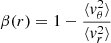 is the anisotropy parameter that quantifies the level of anisotropy of the stellar orbits inside a galaxy. Equation (A.1) thus implies that it is possible to link the kinematic measurements of a galaxy with its total and stellar mass distributions. The mass-follows-light assumption implies that we assume a constant M*/L ratio, which makes it easier to link the luminosity and stellar mass density distributions.
As described in the main body of the paper, we perform kinematic measurements on the cluster members through an IF spectrograph within annular apertures. As shown in Granata et al. (2026), one can obtain the LOS velocity dispersion within an aperture, σap, by weighing the LOS velocity dispersion in Eq. (A.1) with the stellar light distribution within the aforementioned aperture, as
![Mathematical equation: $$ \begin{aligned} \begin{split} \sigma _{\mathrm{ap} }^2(R_1,R_2)=\frac{1}{L(R_1,R_2)}\int _{R_1}^{R_2} 2 \pi R\, I(R)\,\sigma _{\mathrm{LOS} }^2(R)\, \mathrm{d} R=\\ =\frac{4 \pi G}{L(R_1,R_2)}\int _{R_1}^{R_2} R \int _{R}^{\infty } \frac{\nu (r) m(r)}{r^2}\left[\sqrt{r^2-R^2}+ k_{\beta }(r,R)\right]\, \mathrm{d} r\,\mathrm{d} R\,, \end{split} \end{aligned} $$](/articles/aa/full_html/2026/07/aa58758-25/aa58758-25-eq37.gif) (A.2)
(A.2)
where R1 and R2 are, respectively, the internal and external radii of the annulus within which the measurement is performed, and L(R1, R2) = ∫R1R22πR′I(R′) dR′ is the galaxy luminosity within the same annulus. In order to simplify Eq. (A.2), we assume isotropic stellar orbits for the analyzed galaxies, i.e. β(r) = 0. This assumption is justified by the fact that violent collisionless relaxation (Lynden-Bell 1967) is expected to lead to isotropic orbits in the galactic cores (that is, the main region on which we focus our kinematic measurements) and radially biased orbits in the outermost regions (Osipkov 1979; Merritt 1985; Cappellari 2026). Under this assumption, we obtain
 (A.3)
(A.3)
To make these model-predicted LOS velocity dispersion profiles comparable with the observed ones, we need to include the effect of the PSF. To take the PSF into consideration, we sample the LOS velocity dispersion in Eq. (A.1) and the surface brightness of the galaxy, I(R), over a plane, σLOS(x, y) and I(x, y). The extension of the surface on which we perform the sampling is significantly larger than the galaxy angular dimension on the sky, ensuring that the PSF is properly taken into account and that we are not prematurely truncating the models. The 2D profiles are obtained by interpolating over the 1D profiles and exploiting the circular symmetry assumption. The sampling is performed over a grid of 0.01″×0.01″ pixels. The 2D profiles are then convolved with the PSF, modeled as a 2D Gaussian kernel with Full-Width-at-Half-Maximum (FWHM) of 0.6″ and 0.8″ for M0416 and A2744, respectively. Since the PSF acts on the surface brightness profile of each galaxy, the convolution is performed before the light weighting procedure that leads to Eq. (A.3). In order to obtain σap(R1, R2), the light weighing is performed by dividing the sum of the contribution of each pixel lying within the annulus [R1, R2] of the 2D map I(x, y)×σLOS2(x, y) by the sum of the contribution of each pixel within the same annulus of the 2D map I(x, y). The whole procedure can be summarized as
 (A.4)
(A.4)
with
 (A.5)
(A.5)
and
 (A.6)
(A.6)
and where R = x2 + y2 is the distance of each pixel from the galaxy center. This procedure follows Eq. (A.3) and takes into account the fact that we work on a 2D pixel map, practically substituting integrals with sums. From the iteration of Eq. (A.4) on annular apertures of increasing radial size, one can thus obtain a LOS velocity dispersion profile for each galaxy. It is essential to note that when building our dynamical models, we assume that the stars in the cluster members exhibit no ordered motions. This is a good assumption in the central regions of almost all early-type galaxies (ETGs). A rotational velocity contribution would require different assumptions and complicate the modeling. We discussed in the main body the possible effects of a rotational velocity contribution to the measured LOS velocity dispersion profiles and the impact of rotation on the recovered total mass parameter values for the cluster members.
Appendix B: Testing the dynamical model systematics
In this appendix we test the robustness of our dynamical modeling and of our conclusions by adopting different parametrizations for the total and stellar mass density distributions of the cluster members.
All the results discussed in the main body of the paper are obtained by assuming a dPIE-J parametrization to dynamically model the cluster members. Cosmological hydrodynamical simulations often represent the DM structures and substructures in terms of a NFW mass density profile (Navarro et al. 1997). The total mass of a NFW profile within a sphere of radius r can be obtained, integrating the mass density profile, as
![Mathematical equation: $$ \begin{aligned} m(r)=4\pi \rho _0 r_s^3 \left[\text{ ln}\left(\frac{r_s+r}{r_s}\right)-\frac{r}{r_s+r}\right], \end{aligned} $$](/articles/aa/full_html/2026/07/aa58758-25/aa58758-25-eq42.gif) (B.1)
(B.1)
where ρ0 is the central density and rs is a scale radius proportional to the virial radius of the halo, rvir = c × rs, through the concentration parameter c. Dynamical models of cluster members built from Eqs. (4) or (B.1) depend on different free parameters. This implies that the measured values of these parameters obtained by adopting either a dPIE or a NFW profile cannot be compared immediately. However, it is always possible to analyze the maximum circular velocity values obtained with the two mass distributions. For a spherical dPIE profile with a zero core radius, the maximum circular velocity of a galaxy is related to its velocity dispersion as
 (B.2)
(B.2)
Knowing that the maximum circular velocity for a NFW distribution is obtained when r = αrs, with α = 2.16, one obtains
 (B.3)
(B.3)
An alternative choice for the stellar mass density profile is the Hernquist profile (Hernquist 1990), which, under the mass-follows-light assumption, is
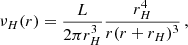 (B.4)
(B.4)
where rH is a scale radius, related to the effective radius as rH = 0.551 Re. We thus built additional dynamical models with the dPIE-H and NFW-J parametrizations and used them to test the systematics of our dynamical modeling and verify the robustness of the measurements of σ0 and rt, as well as our claims. We highlight that using the NFW profile is a first test of the compatibity of the initial prescriptions adopted in simulations with the actual kinematic measurements. We thus ran the inference procedure (see Sect. 3.3) for the 17 galaxies with more than two measured points in their LOS velocity dispersion profiles using the new models. We used the same priors as in the main text for the dPIE-H model and imposed flat priors: ρ0 ∈ [108, 1012] M⊙ kpc−3 and rs ∈ [0.01, 100] kpc for the NFW-J parametrization. We then compared the estimated values of the parameters with those previously obtained with the dPIE-J model. The comparison between the dPIE-J and dPIE-H parametrizations is straightforward, because they only differ in the assumed ν(r), which is fully described by the photometric data and does not need new free parameters. So, we directly compare the measured σ0 and rt posterior distributions. An example of this comparison for one of the sample galaxies is shown in Fig. B.1. From the figure, we notice that the posterior distributions are almost identical. In detail, for 14 of the 17 sample galaxies, the inferred σ0 and rt posteriors completely overlap and are nearly indistinguishable. For the three remaining galaxies, the posterior distributions are still consistent but exhibit small differences, with the dPIE-J model favoring a slightly higher σ0 and a slightly lower rt value. In the top panel of Fig. B.2, we present the measured σ0 values with the dPIE-J and dPIE-H dynamical models for all 17 of the aforementioned galaxies. The red line in the figure represents the one-to-one relation. From the figure, it is clear that the measurements obtained with the two different parametrizations are consistent, given the uncertainties, and are located very close to the one-to-one relation. Moreover, if one estimates the total subhalo mass (Msub) of the galaxies, the values obtained with the two different dynamical models are fully consistent. This implies that the two free parameters, σ0 and rt, can have slightly different values, but some degeneracy ultimately leads to the same measured Msub. In summary, a change in the stellar mass density distribution does not seem to affect the capability of the dynamical models to measure the values of σ0 and rt and reconstruct the observed velocity dispersion profiles. Additionally, a χ2 test can be performed to assess the goodness of fit of the two models in reproducing the measured profiles. This is achieved by generating LOS velocity dispersion profiles for all dynamical models, utilizing the 14000 accepted steps in each MCMC chain, and by searching for the lowest χ2 value to identify the model that best reproduces the measurements. The results of this analysis are shown in Table B.1. Out of the 12 galaxies for which the χ2 analysis prefers a dPIE model, there is no clear preference within the two ν(r) parametrizations. In detail, 5 galaxies are better described by a Jaffe profile, while the remaining 7 are better fit by a Hernquist profile, but the χ2 values are always similar.
 |
Fig. B.1. Comparison of the posterior probability distributions of σ0 and rt obtained from the inference procedure performed on different dynamical model parametrizations for a A2744 cluster member (ID: 38010). We show the dPIE-J and dPIE-H posterior distributions in purple and green, respectively. |
Comparison of the results of the χ2 analysis for the three dynamical model parametrizations for the 17 galaxies with more than two measured points in their LOS velocity dispersion profiles.
The comparison between the dPIE-J model and the NFW-J model is less obvious, since the inference procedure is run on different free parameters. To perform a meaningful comparison, we considered the value of the maximum circular velocity of the galaxies. An example of the comparison between the  distributions for one of the galaxies in our sample is shown in Fig. B.3. From the figure, it is clear that the distributions of the
  values obtained with the two parametrizations are of the same order of magnitude. We evaluated the level of agreement of the maximum circular velocity distributions through the zscore. The results are reported in Table D.1. The distributions of
  are consistent (i.e., zscore ≤ 2.33) for 11 of the 17 sample galaxies with more than two measured kinematic σ values. The inconsistency for the remaining 6 galaxies is related to the small uncertainties of the recovered
  distributions. One can also see in Table D.1 that the galaxies with the largest zscore values are those for which we measure large values of rt. On the bottom of Fig. B.2, we show the correlation between the measurements of
  obtained with the NFW-J and dPIE-J models. The red line represents the one-to-one relation. From the figure, it is evident that the NFW-J model typically predicts slightly higher
  values compared to the dPIE-J model, probably because of the different slopes of the total mass density distributions. One can also observe that the measured values exhibit a small scatter around the one-to-one relation, indicating that the two dynamical models yield similar predictions for
  . The consistency between the two parametrizations implies that our measurements are robust and do not depend significantly on the assumed total mass distribution. It is not possible to directly compare the values of the truncation of the galaxies, since there is no straightforward relation between the two scale radii, rt and rs. Interestingly, the NFW-J model is always able to infer a finite value for both ρ0 and rs. This is probably due to the fact that the scale radius falls at smaller distances from the galactic center than rt and thus can be constrained with less extended kinematic measurements. From Table B.1, it is also possible to see that the χ2 analysis prefers a dPIE over an NFW model for 12 of the 17 galaxies.
 |
Fig. B.2. Comparison of the values of the central stellar velocity dispersion and maximum circular velocity, obtained through different dynamical model parametrizations. Top: correlation between the central stellar velocity dispersion values σ0, obtained from the dPIE-J and dPIE-H dynamical models. Bottom: correlation between the maximum circular velocity |

 |
Fig. B.3. Comparison of the |

The differences in the minimum χ2 values are typically not large enough to conclude on a clearly preferred profile for the total mass density distribution of the cluster members. Interestingly, the NFW-J profile is typically preferred when the measured LOS velocity dispersion profile is flat or slightly increasing in the first two or three measured points. The NFW density profile inner slope can fit the minor increase in the first and innermost velocity dispersion values, making it better at reproducing the kinematic measurements. Moreover, almost all of the measured profiles for which the NFW parametrization is a better fit are influenced by the rotation of the galaxies. Models that take into account both the rotation and the velocity dispersion could thus strenghten the preference toward the dPIE profile. Finally, an additional way to compare the dPIE and NFW parametrizations is through the cumulative total mass profile. As one can see in Fig. B.4, where we show the cumulative total mass as a function of radial distance from the center of a galaxy, the profiles obtained from the dPIE and NFW parametrizations are substantially identical within the maximum radius where we performed the last kinematic measurement,  . Similar results apply to all galaxies in our sample. We remark that with deeper MUSE data (i.e., by radially extending the measured kinematic profiles out to larger
  ), one could find a preferred total mass density profile for cluster members, distinguishing, for instance, between dPIE and NFW.
 |
Fig. B.4. Comparison of the cumulative total mass profiles of a cluster member (ID: 38010) in A2744 obtained with a dPIE-J (cyan) and NFW-J (orange) dynamical models. The inferred median values of rt and rs and the maximum radius of the kinematic measurements, |

Appendix C: The impact of anisotropy on the dynamical models
In this appendix we discuss the effects of anisotropy in stellar orbits on the measured kinematic profiles and on the posterior probability distributions of the parameters inferred from the dynamical models.
As discussed in Appendix A, we modeled the LOS velocity dispersion profiles of cluster members assuming isotropic stellar orbits. This was done by setting β(r) = 0 ∀r in Eq. (A.1). This approximation has often been used to describe ETGs, without impacting the reliability of the measurements performed with dynamical models (Cappellari 2008). Moreover, the isotropic assumption strongly reduces the computational cost of the dynamical models. On the other hand, assuming a fixed value for β is a first order approximation, since ETGs rarely show a constant β over their full extension and have been found to prefer orbits that are more tangentially biased (β ≤ 0) toward their centers and more radially biased (β ≥ 0) in the outskirts (see Fig. 10 in Cappellari 2026). In order to more accurately test the impact of anisotropy on the LOS velocity dispersion profiles and on the σ0 values obtained with our dynamical models, we built some alternative dynamical models based on the full Eq. (A.1), with the dPIE-J parametrization and assuming −0.5 ≤ β(r)≤0.5, ∀r ≤ rkin, and compared their results with the isotropic dynamical models described in the main body of the paper.
We compared the measured profiles to those obtained by assuming different constant β(r) = β values and by fixing σ0 and rt to the median values obtained from the isotropic dPIE-J dynamical models (see Table D.1). In Fig. C.1, we present the comparison between the profiles with β = [0.0, ±0.1, ±0.3, ±0.5], color-coded depending on the β value, and the kinematic measurements, as red points and error bars, for a cluster member (ID: 80726) in M0416. From the figure, one can see how the β = 0 and β = ±0.1 profiles are almost perfectly overlapping. This implies that assuming a small constant value of anisotropy in the stellar orbits of cluster members does not strongly influence the measured values of σ0 and rt. As was shown in Fig. 10 of Cappellari (2026), this is the typical range of values for β(r) at any radial distance from the center of an ETG. Moreover, a χ2 analysis on the predicted profiles with β = 0 and β = ±0.1 leads to similar results. From the figure, one can also see how the profiles with more radially biased stellar orbits, namely β = 0.3 and β = 0.5, reproduce the central measured values the least. On the other hand, one can see that the β = −0.3 profile is similar to the isotropic profile and that assuming extreme tangential anisotropy, such as β = −0.5, does not strongly influence the central values of the LOS velocity dispersion profiles. These results agree with the fact that radially biased orbits are rarely observed in the central regions of ETGs, while massive ellipticals can show tangentially biased orbits in their centers (Binney & Tremaine 2011; Cappellari 2026).
 |
Fig. C.1. Comparison between the measured and model-predicted LOS velocity dispersion profiles for a cluster member (ID: 80726) in M0416 with fixed σ0 and rt and different anisotropy parameter values. The kinematic measurements are shown as red dots while the predictions of the dynamical models are color-coded according to their β value. The scale on the vertical axis is zoomed in, compared to all the other figures in the paper, to show the differences in the profiles that would otherwise be imperceptible. |
In Fig. C.2, we compare the measured profile to those obtained with constant β(r) = β values (with same color coding as in Fig. C.1), the same fixed rt as before; and σ0 set in order for the profiles obtained with each dynamical model to fit the first kinematic measurement. This is done to probe the effects that different anisotropy values have on the predictions of dynamical models that are forced to reproduce the measured central stellar velocity dispersion. In detail, we set σ0 = 241.9 km s−1 (as in Table D.1) for β = [0.0, ±0.1, −0.3], σ0 = 234.9 km s−1 for β = 0.3, σ0 = 244.9 km s−1 for β = −0.5 and σ0 = 211.9 km s−1 for β = 0.5. From the figure, it is evident that the profiles with β = 0, ±0.1 accurately reproduce the kinematic measurements, while the dynamical models worsen at reproducing the measured profiles for increasing |β| values. To avoid this, one should assign increasingly higher values of rt at increasingly larger values of |β|. A χ2 analysis on the LOS velocity dispersion profiles shows that the β = 0 and β = ±0.1 parametrizations, as before, are the ones that better reproduce the kinematic measurements. Moreover, comparing the σ0 values we manually set for each dynamical model, one can see how assuming low and plausible values of anisotropy does not require changing the values of the kinematic parameters in order for the model to reproduce the measured profile. This implies that the dynamical models are able to infer the values of σ0 and rt, independently of the anisotropy, as long as the assumptions on β are realistic.
 |
Fig. C.2. Comparison between the measured and model-predicted LOS velocity dispersion profiles for a cluster member (ID: 80726) in M0416 with fixed rt and different anisotropy parameter values. The σ0 value is manually fixed such that all of the model-predicted profiles show the same central σ value. The profiles are color-coded as in Fig. C.1. |
Finally, we developed a full dPIE-J anisotropic dynamical model to test the effects of anisotropy on the inferred values of σ0 and rt. In this model, β is constant at all radii and the MCMC optimization process (see Sect. 3.3) is performed on σ0 and rt with priors defined as in the main body of this paper. Given that a full model has a higher computational cost than an isotropic model, we adopted MCMC chains of 2000 steps each, with initial σ0 and rt values set as the values obtained from the isotropic models (see Table D.1). We ran the dynamical model assuming six different values of the anisotropy parameter, namely β = [ ± 0.1, ±0.2, ±0.3], and compared the resulting posterior probability distributions with those of the isotropic dynamical models. The comparison of the posterior probability distributions of σ0 and rt for one galaxy (ID: 83064) in M0416 is shown in Fig. C.3. The median values obtained with the isotropic model are shown as blue lines. From the figure, it is evident that all the posterior distributions are similar and that the inferred median values are consistent with the reference isotropic model, regardless of the assumed β value. Our analysis demonstrates that assuming isotropy or small and constant anisotropy parameter values to describe ETG stellar orbits does not significantly impact the predictions of our dynamical models. This result confirms the robustness of our modeling methods and measurements, thereby strengthening the conclusions of this paper. Similarly to us, Liang et al. (2026) find that assuming isotropic profiles or the Osipkov-Merritt (Osipkov 1979; Merritt 1985) model to define β(r) does not impact the inferred galaxy mass density distributions. In future works, more complex dynamical models could consider a full functional form for the anisotropy parameter β(r) or define β as a free parameter to be inferred.
 |
Fig. C.3. Comparison of the σ0 and rt posterior probability distributions obtained with different anisotropy values. We plot the values of the two parameters obtained from the isotropic dPIE-J dynamical model as blue lines. Each posterior distribution is color-coded, depending on the value of the anisotropy parameter assumed in the inference procedure. |
Appendix D: Sample and main physical parameters
In this appendix we present our sample of cluster members, including their redshift and structural parameters, as described in Tortorelli et al. (2023) for the galaxies in A2744 and M0416, respectively. A further analysis was presented in Granata et al. (2026). We also present the relevant measurements that were used to build the dynamical models and calibrate the scaling relations discussed in the main body of the paper.
Relevant measurements and values for the 17 cluster members with more than two measurements in their LOS velocity dispersion profiles.
Relevant measurements and values for the galaxies with fewer than three measured points in their LOS velocity dispersion profiles.
All Tables
Comparison of the parameters of the F-J scaling relation obtained from the dynamical models, the SL models optimizations, and previous literature kinematic measurements, for the clusters of galaxies A2744 and M0416.
Comparison of the results of the χ2 analysis for the three dynamical model parametrizations for the 17 galaxies with more than two measured points in their LOS velocity dispersion profiles.
Relevant measurements and values for the 17 cluster members with more than two measurements in their LOS velocity dispersion profiles.
Relevant measurements and values for the galaxies with fewer than three measured points in their LOS velocity dispersion profiles.
All Figures
|
Fig. 1. Spectrum of the cluster galaxy 80726 in M0416, extracted from a circular aperture with radius r = 0.5″ centered on the galaxy luminosity center. The black line shows the measured spectrum, while the red line shows the fit spectrum, obtained with the pPXF pipeline, from rest-frame 3700–5100 Å. On the bottom, the residuals between the two spectra are shown as green dots. The gray bands highlight masked regions. On the top, the values of the extracted kinematic parameters are listed: the velocity dispersion, σ, and the peculiar velocity, v, in kilometers per second, with their corresponding uncertainties, and the average signal-to-noise ratio ⟨S/N⟩. |
| In the text | |
|
Fig. 2. MUSE cube cutout of the galaxy 80726 in the cluster of galaxies M0416. The annuli of 0.5″ width and increasing radial size, within which the LOS velocity dispersion profile was measured, are shown. |
| In the text | |
|
Fig. 3. Measured LOS velocity dispersion profile of galaxy 80726 as a function of the radial distance from the center, in both arcseconds (bottom) and kiloparsecs (top). The red lines along the horizontal axis show the uncertainty on the measurement position due to each annulus width, as shown in Fig. 2, while the ones along the vertical axis represent the uncertainty on each measured σLOS, obtained from the pPXF pipeline. |
| In the text | |
|
Fig. 4. Corner plot obtained from the inference procedure on the cluster galaxy 83064 in M0416. The posterior probability distributions for σ0 and rt and their correlation are shown. The median values and 16th and 84th percentiles are reported at the top and highlighted with blue and green lines. |
| In the text | |
|
Fig. 5. Comparison between measured and model-predicted velocity dispersion profiles. In black, we show the profile obtained from the kinematic measurements (red data points) of the cluster member 83 064 in M0416. As solid orange lines, we plot 100 profiles obtained with the dynamical model by sampling the posterior distributions of the free parameters, drawn from the MCMC optimization and shown in Fig. 4. The distance from the galactic center is reported in arcseconds (bottom) and kiloparsecs (top). |
| In the text | |
|
Fig. 6. Corner plots of the central stellar velocity dispersion, σ0, and truncation radius, rt, for two cluster members (38 729 on the left and 34 423 on the right) in A2744, obtained from the inference procedure. The posterior probability distributions of σ0 and rt and their correlations are shown. The median values and percentiles are highlighted as in Fig. 4. The rt posterior probability distributions for these galaxies are classified as flat and tailed, respectively. The σ0 posterior distribution is close to a Gaussian distribution for both galaxies. |
| In the text | |
|
Fig. 7. Comparison between the measured, SL, and dynamically modeled velocity dispersion profiles for a M0416 cluster member (ID: 83064). In black, we plot the measured kinematic profile. In orange, we show 100 profiles obtained with the dPIE-J dynamical model. In green and blue, we plot 100 profiles obtained from the calibrated and optimized F-J scaling relations from B+21 and B+23b, respectively. The uncertainties and the distance are defined as in Fig. 3. |
| In the text | |
|
Fig. 8. Comparison between kinematic measurement (RS sample in Table 1) and dynamical model F-J scaling relations for the clusters of galaxies A2744 (on the left) and M0416 (on the right). In green, we plot the MCMC best-fitting F-J scaling relations obtained from B+23a and B+21. In orange, we present the best-fitting F-J scaling relations of our dynamical model. The measured kinematic and dynamical σ values (σ0 in our models) are reported as blue and red dots, respectively, with measured uncertainties as error bars. The total number of galaxies in the RS sample for each cluster is shown in the top right corner. We also illustrate the maximum likelihood relations as dotted black lines. |
| In the text | |
|
Fig. B.1. Comparison of the posterior probability distributions of σ0 and rt obtained from the inference procedure performed on different dynamical model parametrizations for a A2744 cluster member (ID: 38010). We show the dPIE-J and dPIE-H posterior distributions in purple and green, respectively. |
| In the text | |
|
Fig. B.2. Comparison of the values of the central stellar velocity dispersion and maximum circular velocity, obtained through different dynamical model parametrizations. Top: correlation between the central stellar velocity dispersion values σ0, obtained from the dPIE-J and dPIE-H dynamical models. Bottom: correlation between the maximum circular velocity |
| In the text | |
|
Fig. B.3. Comparison of the |
| In the text | |
|
Fig. B.4. Comparison of the cumulative total mass profiles of a cluster member (ID: 38010) in A2744 obtained with a dPIE-J (cyan) and NFW-J (orange) dynamical models. The inferred median values of rt and rs and the maximum radius of the kinematic measurements, |
| In the text | |
|
Fig. C.1. Comparison between the measured and model-predicted LOS velocity dispersion profiles for a cluster member (ID: 80726) in M0416 with fixed σ0 and rt and different anisotropy parameter values. The kinematic measurements are shown as red dots while the predictions of the dynamical models are color-coded according to their β value. The scale on the vertical axis is zoomed in, compared to all the other figures in the paper, to show the differences in the profiles that would otherwise be imperceptible. |
| In the text | |
|
Fig. C.2. Comparison between the measured and model-predicted LOS velocity dispersion profiles for a cluster member (ID: 80726) in M0416 with fixed rt and different anisotropy parameter values. The σ0 value is manually fixed such that all of the model-predicted profiles show the same central σ value. The profiles are color-coded as in Fig. C.1. |
| In the text | |
|
Fig. C.3. Comparison of the σ0 and rt posterior probability distributions obtained with different anisotropy values. We plot the values of the two parameters obtained from the isotropic dPIE-J dynamical model as blue lines. Each posterior distribution is color-coded, depending on the value of the anisotropy parameter assumed in the inference procedure. |
| In the text | |
Current usage metrics show cumulative count of Article Views (full-text article views including HTML views, PDF and ePub downloads, according to the available data) and Abstracts Views on Vision4Press platform.
Data correspond to usage on the plateform after 2015. The current usage metrics is available 48-96 hours after online publication and is updated daily on week days.
Initial download of the metrics may take a while.