


| Issue |
A&A
Volume 711, July 2026
|
|
|---|---|---|
| Article Number | A126 | |
| Number of page(s) | 14 | |
| Section | Extragalactic astronomy | |
| DOI | https://doi.org/10.1051/0004-6361/202558583 | |
| Published online | 08 July 2026 | |
Identification of periodicities with arbitrary shapes in light curves of active galactic nuclei
1
Università degli Studi di Milano-Bicocca, Piazza della Scienza 3, 20126 Milano, Italy
2
INFN, Sezione di Milano-Bicocca, Piazza della Scienza 3, I-20126 Milano, Italy
3
INAF – Osservatorio Astronomico di Brera, Via Brera 20, I-20121 Milano, Italy
4
Department of Physics and Astronomy, Washington State University, Pullman, WA 99163, USA
5
Institute of Astrophysics, FORTH, GR-71110 Heraklion, Greece
6
Institute for Gravitational Wave Astronomy & School of Physics and Astronomy, University of Birmingham, Birmingham B15 2TT, UK
7
Como Lake centre for AstroPhysics (CLAP), DiSAT, Università dell’Insubria, Via Valleggio 11, 22100 Como, Italy
8
Department of Physics & Astronomy, Vanderbilt University, Nashville, TN 37240, USA
9
Department of Life and Physical Sciences, Fisk University, Nashville, TN 37208, USA
★ Corresponding author: This email address is being protected from spambots. You need JavaScript enabled to view it.
Received:
15
December
2025
Accepted:
21
May
2026
Abstract
Massive black hole binaries are expected to be observable as periodic active galactic nuclei in time-domain photometric surveys. Periodicities may originate from different physical processes, including the intermittent gas feeding of the black holes caused by the time-varying non-axisymmetric binary potential, the Doppler boosting of the flux emitted by individual accretion discs bound to the orbiting black holes, and the gravitational lensing of the accretion disc of one black hole by another such disc. Only the Doppler boost scenario applied to circular binaries with non-modulated accretion predicts a sinusoidal light curve, while in the general case, binary signals are expected to show more complex periodic patterns. Current searches for massive black hole binaries rely on techniques tailored to quasi-sinusoidal light curves, but fail to identify the more complex predicted periodicities. We present an alternative method that leverages Gaussian processes, making use of a generic periodic kernel that is flexible enough to identify arbitrary periodicities in unevenly sampled light curves with realistic quasar noise. We demonstrate that it outperforms previously proposed strategies in identifying general periodicities by analysing mock light curves with different baselines. Specifically, our analysis can detect non-sinusoidal periodicities (e.g. sawtooth-shaped or symmetric flares) and retrieves a higher fraction of true periodicities when compared to a periodogram analysis or a Gaussian process analysis with less flexible periodic kernels. Furthermore, by comparing the retrieved fraction of periodicities between mock Palomar transient factory light curves and mock Legacy Survey of Space and Time light curves, we found that our analysis is most sensitive to the number of observed cycles. The application of this analysis has the potential to greatly increase the scientific return of current and upcoming large time-domain photometric surveys.
Key words: methods: data analysis / methods: statistical / techniques: photometric / galaxies: interactions / quasars: supermassive black holes
© The Authors 2026
 Open Access article, published by EDP Sciences, under the terms of the Creative Commons Attribution License (https://creativecommons.org/licenses/by/4.0), which permits unrestricted use, distribution, and reproduction in any medium, provided the original work is properly cited.
This article is published in open access under the Subscribe to Open model. This email address is being protected from spambots. You need JavaScript enabled to view it. to support open access publication.
1. Introduction
Since every galaxy is expected to host a massive black hole (see Kormendy & Gebhardt 2001), massive black hole binaries (MBHBs) are considered the natural outcome of galaxy mergers (Begelman et al. 1980). If the interaction with their local environment is effective in removing orbital energy and angular momentum, MBHBs can reach separations that are small enough and emit low-frequency gravitational waves. These can be detectable by ongoing pulsar-timing array (PTA) campaigns (Verbiest et al. 2016) and by future space-based interferometers such as the Laser Interferometer Space Antenna (LISA, see Amaro-Seoane et al. 2017, 2023). These binaries are also expected to emit bright electromagnetic signals that can be used to detect them. Multiple observational features identifying MBHB candidates have been proposed (see Dotti et al. 2012; De Rosa et al. 2019; Bogdanović et al. 2022; D’Orazio & Charisi 2023 for an overview, and Gaskell 1988; Dotti et al. 2022, 2023; Chan et al. 2025; Bertassi et al. 2025 for alternative signatures). The electromagnetic identification of MBHBs can complement the interpretation of the (still tentative) detection of a gravitational wave background in PTA data (EPTA Collaboration 2023; Agazie et al. 2023; Reardon et al. 2023; Xu et al. 2023), and constrain the highly uncertain rates of MBHB coalescences detectable by LISA (e.g. Fiacconi et al. 2013; del Valle et al. 2015; Souza Lima et al. 2017; Bortolas et al. 2020, 2022).
At small separations, corresponding to MBHB orbital periods of a few years, a promising feature for the identification of active MBHBs is the quasi-periodic modulation of their brightness. Depending on the binary intrinsic properties, this modulation can be driven by (i) the time-varying non-axisymmetric potential of the binary, prompting intermittent gas feeding from the outer circumbinary disc (MacFadyen & Milosavljević 2008; Hayasaki et al. 2008), (ii) the phase-dependent Doppler boosting of the flux emitted by the individual accretion discs bound to the individual BHs (mini discs) that move with relativistic velocities (D’Orazio et al. 2015), and/or (iii) the gravitational lensing of the accretion disc of one black hole due to the gravitational potential of the companion (D’Orazio & Di Stefano 2018; Kelley et al. 2021). Periodicities due to the presence of MBHBs can also be found when both MBHs are inactive. For instance, when a luminous star lies behind an MBHB, it can be periodically gravitationally lensed by the binary (see Wang et al. 2026)1.
Hundreds of close MBHB candidates have already been selected based on the apparent periodicity of their light curves in time-domain photometric surveys (see Graham et al. 2015; Charisi et al. 2016; Liu et al. 2019; Chen et al. 2020; Li et al. 2023; Chen et al. 2024; Foustoul et al. 2025; Tubín-Arenas et al. 2025). The natural variability of active galactic nuclei, characterised by red noise, that is, a noise that shows a higher power at long timescale variability (see Ulrich et al. 1997), can mimic periodic light curves over a few (apparent) cycles (see Vaughan et al. 2016; Witt et al. 2022; El-Badry et al. 2026). Thus, it is imperative to quantify the statistical evidence in favour of periodic signals when compared to a red-noise model component alone. Upcoming time-domain photometric surveys, such as the Legacy Survey of Space and Time (LSST, see Ivezić et al. 2019) and the Nancy Grace Roman Space Telescope (see Haiman et al. 2023), have the observational length, depth, and light-curve sampling frequency needed to identify close-separation MBHB candidates (see e.g. the discussions in Kelley et al. 2019; Xin & Haiman 2021; Kelley et al. 2021; Haiman et al. 2023).
All the above-mentioned searches for periodic light curves (with the exception of Foustoul et al. 2025, as discussed in what follows) are based, at least in the pre-selection of the candidates, on the analysis of Lomb-Scargle periodograms (LSP, see Lomb 1976; Scargle 1982; VanderPlas 2018), which are a generalisation of the Fourier transform power spectrum for unevenly sampled time series2. The LSP-based analysis has three main limitations: (i) the general distribution of the periodogram peaks is not known (limiting our ability to estimate the likelihood of a period), (ii) the independence of the specific powers in each frequency bin is not guaranteed (e.g. Covino et al. 2022; Lin et al. 2026), and, most importantly, (iii) non-sinusoidal periodic signals will spread power over multiple frequencies, making the identification of a single statistically significant peak in the power spectrum more challenging. While points (i) and (ii) only apply to unevenly sampled light curves (for which the LSP cannot be constructed directly through a Fourier transform), point (iii) applies to the unrealistic scenario of evenly spaced observations as well. Lin et al. (2026) indeed showed that in the presence of realistic quasar noise, LSP-based searches identify only ≲40% of sinusoidal signals (for which they are best suited) and ≲10% of more complex (sawtooth-shaped) periodic signals. This is particularly relevant because only Doppler boosting of circular binaries with non-modulated accretion can produce sinusoidal light curves. All other physical mechanisms of periodicity instead show more complex and irregular profiles (see Hu et al. 2020; Duffell et al. 2020; Zrake et al. 2021; Westernacher-Schneider et al. 2022; Cocchiararo et al. 2024).
A few periodic light-curve searches have been published that were not based on the LSP (see Covino et al. 2020; Zhu & Thrane 2020; Rigamonti et al. 2025 for applications to single objects and Foustoul et al. 2025 for larger searches). Therein, light curves are modelled directly in the time-domain through Gaussian processes (GPs, see Rasmussen & Williams 2006; Aigrain & Foreman-Mackey 2022), for which a likelihood, and hence, the evidence of a periodic model, is well defined. However, the reliability of the evidence depends on the validity of the assumed noise model. The GP kernel associated with a periodic model is often described by a simple cosine function. As detailed in Section 2, this prevents a GP model from modelling sudden jumps in the light curves over timescales shorter than the period, P. We note that the GPs have already been applied in AGN studies, for example, in searching for flares (see McLaughlin et al. 2024), and intrinsic variability studies (see Zhang et al. 2023, 2024; Yu et al. 2026)
We present an alternative analysis based on light-curve modelling through GPs, assuming a more flexible family of periodic kernels, as proposed by Durrande et al. (2016). We test them on realistic (periodic and non-periodic) AGN light curves, including the effect of red noise. We show that when GPs are coupled with a robust Bayesian treatment, they allow us to detect complex and irregularly shaped light curves. We note that another appealing approach to searching for periodicities in astrophysical light curves is the use of deep-learning models and neural networks (see Miller et al. 2024; Fernandes et al. 2025, for two examples), and indeed, such techniques are being applied to real and mock AGN periodic light curves (see Kovačević et al. 2023). Different from these methods, the GP analysis we propose can directly link the kernel parameters to the properties of the light curve, such as the amplitude, shape, and period, and it can estimate the parameters of the intrinsic variability as a natural byproduct. In Section 2 we discuss the periodicity detection algorithm and compare various GP kernels. In Section 3 we identify a detection statistic and an optimal threshold in the identification of periodicities. We discuss the fraction of retrieved periodicities and the goodness of the parameter estimation. Finally, we discuss which parameters affect the retrieved fractions most and compare our findings with alternative methods in the literature. In Section 4 we summarise our conclusions.
2. Search algorithm
Gaussian processes, typically denoted as 𝒢𝒫(m(t),k(t, t′)), with t and t′ referring to two times of observation, are stochastic processes defining distributions over functions, such that for any finite collection of inputs the corresponding function values have a joint multivariate Gaussian distribution,
 (1)
(1)
where mi = m(ti, θ) is the mean function, and Kij = k(ti, tj, ϕ), where Kij is the covariance matrix, while k(ti, tj, ϕ), thought of as a function over continuous (t, t′), is the covariance function (or kernel). Here, t = [t1, …, tn] is the set observation timestamps, while θ, ϕ are the so-called process hyperparameters. The covariance function of a GP is defined so that the associated K is symmetric (i.e. K(ti, tj) = K(tj, ti)) and positive semi-definite.
The great advantage of GPs over alternative models is that when a set of data points is collected, posterior predictions over the observed domain are readily available analytically,
![Mathematical equation: $$ \begin{aligned} \begin{split} \boldsymbol{\mu }_*&= {\boldsymbol{K}}(\mathbf t _*, \mathbf t ) \, [\boldsymbol{K}(\mathbf t , \mathbf t ) + \sigma _n^2 \mathbf I ]^{-1} \, \mathbf y \\ \boldsymbol{\Sigma _*}&= {\boldsymbol{K}}(\mathbf t _*, \mathbf t _*) - \boldsymbol{K}(\mathbf t _*, \mathbf t ) \, [\boldsymbol{K}(\mathbf t , \mathbf t ) + \sigma _n^2 \mathbf I ]^{-1} \, \boldsymbol{K}(\mathbf t , \mathbf t _*), \end{split} \end{aligned} $$](/articles/aa/full_html/2026/07/aa58583-25/aa58583-25-eq2.gif) (2)
(2)
where t* is the vector containing the times at which we wish to predict the values of the light curve, t is the vector of the times used to fit the hyperparameters of the kernel, K(t, t) is the kernel computed on the points used to fit the GP, K(t*, t) is the covariance between t and t*, σn is the photometric error of each data point, μ* is the predicted mean, Σ* is the prediction covariance, and finally, I is the identity matrix. We only used GPs to fit the best hyperparameters describing the noise and the periodic signal, and not for predictive purposes.
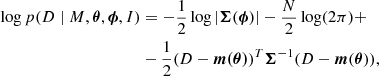
When the mean and covariance functions are specified (e.g. for stationary Gaussian processes, the covariance function is simply related via the Fourier transform with the power spectral density; see Foreman-Mackey et al. 2017), we can fit the set of hyperparameters θ, ϕ that describe the data D. The log-likelihood of the data is given by (see Rasmussen & Williams 2006)
 (3)
(3)
where N is the number of observations, and Σij = Kij + σiδij, where K and m are the covariance matrix and mean function, δij is the Kronecker delta, and σi denotes the observation noise variance at input ti.
The evidence (or marginal likelihood)3 of a particular model given a set of data is defined as
 (4)
(4)
where p(D|M, θ) is the likelihood function introduced in Eq. (3), and p(θ|M) denotes the prior. In our context, the data D consist of the observed light curve (ti, Mi), with i = 1, 2, …N labelling the data points and Mi being the magnitude observed at time ti. Finally, M is the considered model, and θ are the hyperparameters associated with it. Within the above formalism, the outcome of a model comparison is quantified by the so-called Bayes factor, that is, the evidence ratio of two competing models, B = Zmodel, 1/Zmodel, 2. As we show in Section 2.4, it strongly depends on the assumed kernel in each model.
Below, we briefly introduce three kernels that were used to describe either random intrinsic AGN variability (exponential kernel) or periodicities (cosine and periodic kernels; the latter are well suited to periodic signals of arbitrary shape). To model the noise and the periodic signal in the light curve, we constructed kernels as the sum of periodic and exponential kernels.
2.1. Exponential kernel
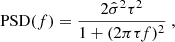
The intrinsic AGN variability in the optical and UV bands is well described by damped random walk (DRW, see Kelly et al. 2009; MacLeod et al. 2010; Kozłowski et al. 2010) and is parametrised by a damping timescale τ, which represents the light-curve autocorrelation timescale, and a variability amplitude,  , which quantifies the typical magnitude of intrinsic variations. Therefore, the process power spectral density (PSD) reads
 (5)
(5)
where f denotes the frequency. This stochastic process can be equivalently described by the kernel
 (6)
(6)
2.2. Cosine kernel
The GPs can be used to model periodic signals. This can be done by employing a periodic mean function (e.g. m(t) = Asin(2πt/P)), with P being its fundamental period, and modelling the noise through the covariance matrix, for example using the kernel defined in Equation (6) to describe red noise. Alternatively, the periodic component can be directly incorporated in the noise term of the covariance matrix. We followed the second approach because a deterministic analytical description of the expected modulation from the interaction with the gas surrounding the binary is still unavailable, and we assumed a constant mean function equal to 0 (m(θ) = 0).
Sinusoidal signals can be modelled using the cosine kernel (see Section 3.2), which reads
 (7)
(7)
where A is the autocorrelation strength, and P is its period.
As the correlation between two photometric points with Δt ≪ P is always close to 1 by construction, the cosine kernel fails to model sudden jumps in the light curves on timescales shorter than P properly.
2.3. Generic periodic kernel
We employed a more generic periodic kernel that was flexible enough to model periodic signals of arbitrary shapes. It is defined by
 (8)
(8)
The hyperparameter l determines how rapidly correlations decay as the distance between two points increases within a period. We note that a similar kernel was used to study stellar variability, exoplanetary science and eclipsing binary characterisation (see Haywood et al. 2014; Vanderburg et al. 2015; Angus et al. 2018; González-Álvarez et al. 2021; Wang et al. 2025, and references therein for applications). However, in these works, the kernel is quasi-periodic (the periodic kernel is multiplied by an exponential decay) and not the purely periodic kernel we assumed here.
Unlike the cosine kernel, whose Fourier expansion over Δt consists of a single Fourier component at frequency f = 1/P, which limits it to a single sinusoidal term, the periodic kernel can be expanded in an infinite Fourier series over Δt = |ti − tj|. For this reason, it can describe periodicities with arbitrary shapes.
The contribution of each harmonic was weighted by the kernel length scale l: lower values of l upweight higher harmonics and allow for sharp edges in the signal, while higher values of l downweight them, yielding smoother, nearly sinusoidal signals. A more detailed discussion of this point is reported in Appendix A. Through the higher-dimensional parameter space and a different functional form, the generic periodic kernel is suitable to describe signals with a higher complexity than the cosine kernel. Therefore, it is only through Bayesian model selection that we are able to assess whether this complexity is supported by observed data.
Figure 1 shows the posterior predictive distributions defined in Equation (2) for idealised mock signals: a sinusoid (upper panel) and a sawtooth signal (lower panel), evenly sampled with a daily cadence. The two examples were fitted using the cosine kernel (Eq. 7) and the periodic kernel (Eq. 8). The two kernels accurately describe the sinusoidal light curve, as can be seen from the upper panel of Figure 1, where the solid lines and shaded regions clearly show that both the periodic and cosine kernels can reproduce the sinusoidal signal as they overlap. For the sawtooth light curve, both kernels recover the correct period, but only the periodic kernel captures the true shape of the signal. This can be seen from the bottom panel of Figure 1, which highlights both the inadequacy of the cosine kernel in modelling non-sinusoidal light curves and the flexibility of the periodic kernel that allows it to describe periodicities with arbitrary shapes. This distinction is important for the model comparison because the Bayes factor in favour of the cosine kernel in the sawtooth case would be suppressed. Specifically, we found log10(Zperiodic/Zcosine)∼ − 5 for the sinusoidal light curve, as expected, because the two models accurately describe the sinusoidal shape, but the cosine kernel requires one parameter less than the periodic kernel. On the other hand, for the sawtooth light curve, we obtained log10(Zperiodic/Zcosine)∼100, highlighting the fact that the cosine kernel is not suitable for describing such signals. In the following analysis, we adopt the generic periodic kernel, while comparisons with the cosine kernel and with the LSP analysis are discussed in Sections 3.2 and 3.5, respectively.
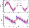 |
Fig. 1. Posterior predictive distributions from GP inference on a sinusoidal light curve (upper panel) and a sawtooth light curve (lower panel). The results from the cosine kernel (Equation 7) are shown in red, and those from the periodic kernel (Equation 8) are plotted in blue. The shaded regions indicate the 1σ (dark) and 2σ (light) credible intervals. |
2.4. Model selection
We searched for the GP hyperparameters through Bayesian inference, obtaining posterior samples with nested sampling (see Skilling 2006). Nested sampling is a statistically robust algorithm suitable for the estimation of the model parameters (or hyperparameters, in the context of GPs) and the associated uncertainty, in the form of posterior samples. In addition, it directly provides an estimate of the model evidence. More specifically, we used Gpytorch (Gardner et al. 2021) to construct the GP kernel and to evaluate the likelihood. For the nested-sampling algorithm, we used the raynest implementation (see Veitch et al. 2024) with 500 live points, and the stopping was set so that the evaluation stopped as soon as the increment of the log-evidence was smaller than lnZ < 0.1.
In the following, we compare two models: a pure noise model given by the exponential kernel defined by Equation (6), and a model that includes a periodic modulation and noise, described by the sum of kernels in Equations (6) and (8).
To ensure that the priors were sufficiently broad for a proper posterior sampling across all objects, we rescaled the light curves. Specifically, we subtracted the mean and divided by the standard deviation of each quantity. This was done for the times and magnitudes of the light-curve data4.
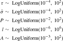
We assumed log-uniform priors for all the rescaled GP hyperparameters.
Noise model:
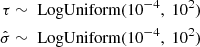
Periodic model:
We calculated the Bayes factor between the periodic+noise and noise-only models to select the model that described the data best.
We fixed the Bayes factor threshold to claim the detection of a periodicity by determining the distribution of the Bayes factor produced by noise-only realisations (see Section 3.1).
2.5. Simulations of mock light curves
We analysed light curves consisting of a periodic signal superimposed on realistic quasar noise (modelled as a DRW). The periodic signal is characterised by three parameters: the period P, the amplitude A, and the phase ϕ, while the noise is described by a damping timescale τ and an amplitude σ for a total of five parameters used to generate each light curve.
We used the same light curves as Lin et al. (2026), where periodicity-related parameters were uniformly sampled from [0, 0.5), [0,Tdata/1.5), and [0, 2π) for A, P, and ϕ, respectively, and with Tdata being the baseline of the respective PTF light curve. Parameters associated with the intrinsic AGN variability were derived from each quasar property based on the correlations from MacLeod et al. (2010; see Lin et al. 2026, for full details).
For each set of input parameters, four types of light curves are generated. The periodic component was allowed to either have a sinusoidal or a sawtooth-like shape, and the observational baseline was constructed with different cadences: PTF-like (with the same cadence as the one of the Palomar Transient Factory) or idealised (sampled daily). The PTF-like light curves were constructed using the same cadence as those analysed in Charisi et al. (2016). We assigned to each point photometric errors sampled from a Gaussian distribution with zero mean and a standard deviation equal to the photometric uncertainty of the corresponding point in the real PTF light curve. For the idealised light curves, photometric errors were added analogously, but with a standard deviation equal to the mean photometric error of the corresponding PTF light curve (see Lin et al. 2026, for additional details). The typical mean photometric error associated with real PTF light curves is ∼0.05.
We complemented our analysis with 2000 additional LSST-like light curves from Lin et al. (2026) (1000 with a sinusoidal variability and 1000 with sawtooth luminosity profiles). We selected this sub-set of light curves based on the analysis of the PTF-like light curves, for which the periodicity was not detected.
These light curves were generated using the same parameters as in the PTF-like ones, but assuming an LSST-like cadence, magnitude uncertainties, and an extended baseline of equal to the expected survey duration, Tobs ∼ 10 yr. Specifically, LSST-like light curves had a median cadence of around 5 days, with seasonal gaps of approximately 4 months each year, and showed a median uncertainty of 6.5 × 10⁻³ mag, which is smaller by an order of magnitude than the PTF-like and ideal ones. In Figure 2 we show one example light curve for each baseline (the LSST baseline in the main plot and the ideal and PTF baselines in the inset). We emphasise that we limited ourselves to only 1000 LSST-like light curves for each periodic signal (instead of the total 12 400 analysed in Lin et al. 2026 and above) due to the computational cost of the analysis; a complete analysis of a single LSST-like light curve takes up to 8 hours. In Section 4 we discuss possible ways to speed the code up in order to address this significant limitation of our method, which prevented us from scaling our calculations to large quasar samples.
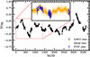 |
Fig. 2. Examples of the same sampled sinusoidal light curve for the three baselines. The LSST light curve is shown in the main panel, and the PTF (blue points) and ideal (orange points) light curves are displayed in the inset (lower right). The dashed red rectangle in the main panel highlights the typical duration of the PTF and ideal sampling, emphasising the longer observational coverage of the LSST baseline. |
3. Results
In this section, we present the results of the analysis of 12 400 light curves for each combination of short baselines (PTF-like and idealised) and the shape of the periodicity (sinusoidal and sawtooth), as well as a subsample of 1000 LSST-like light curves for each periodicity shape.
3.1. Bayes factor threshold for a periodicity detection
To assess whether a light curve shows significant evidence of periodicity, it is necessary to set a threshold in the Bayes factor obtained by the comparison between the noise-only and the periodic+noise models. We set this threshold in two ways. The first way was based on fixing the false-positive rate. Specifically, we set this threshold by finding a Bayes factor threshold based on the false-positive rate assumed in Lin et al. (2026) to make a fair comparison that is discussed in Section 3.5. The second way was based on the ROC curve. Specifically, we set this threshold by finding the value of the Bayes factor that maximises the distance from the curve describing random classification. The main results we discuss here were obtained through the ROC-based threshold, as it maximises the efficiency of periodicity detection by keeping the false-positive rate (the fraction of non-periodic signals that are misidentified as periodic) low. We characterised the FAP by generating 4 × 12 400 noise-only light curves (12 400 light curves for each of the four combinations of sinusoidal and sawtooth signals for the idealised and PTF-like data). Specifically, we computed the Bayes factor between the noise-only and periodic+noise models for all the noise-only light curves and obtained their distribution.
In Figure 3 we show the cumulative distribution of log10B for all three sampling scenarios for the periodic kernel: PTF-like (blue distribution), idealised (orange distribution), and LSST-like (green distribution).
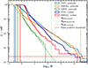 |
Fig. 3. Distribution of the Bayes factors for the 104 noise-only light curves for the PTF using the periodic kernel and cosine kernel (blue and dark blue distributions) and ideal using the periodic kernel and cosine kernel (orange and red distributions) baselines, and the 103 noise-only light curves for the LSST (green distribution) baseline found by analysing the light curves with the generic periodic kernel. The vertical lines refer to the Bayes factor threshold identified for a fair comparison with the LSP analysis discussed in more detail in Section 3.5. |
From the distributions in Figure 3, we retrieved the threshold on the Bayes factor to obtain an FAP < 25 × 10−5 that allows for a fair comparison with the LSP analysis (see Section 3.5)5. These thresholds were found between log10B = 4 − 5 for the ideal and PTF-like light curves and between log10B = 2 − 3 for LSST-like light curves. To be conservative, we assumed a Bayes factor threshold of log10B = 5 for ideal and PTF-like light curves and of log10B = 3 for LSST-like light curves when comparing our results with the LSP-analysis presented in Section 3.5.
The true-positive fraction was computed by dividing the number of periodic light curves that were correctly identified as periodic by the total number of periodic light curves we analysed. These fractions are shown in Figure 4.
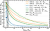 |
Fig. 4. Fraction of the realisation containing periodic signals with a Bayes factor greater than a threshold as a function of the assumed threshold. The solid lines show the sinusoidal light curves, and the dotted lines show sawtooth light curves. Orange, blue and green show the ideal, PTF, and LSST baselines, respectively. The vertical lines show the Bayes factor threshold of log10Btrs = 5 for the ideal, PTF (solid line), and log10Btrs = 3 for the LSST baseline (dashed line) used to compare the results with the LSP analysis (see Section 3.5). The circles and squares identify the points at the identified ROC curve-based Bayes threshold for the sinusoidal and sawtooth cases, respectively. The orange markers show ideal-like light curves, blue markers show PTF-like light curves, and finally, green markers show LSST-like light curves. |
The distributions in Figures 3 and 4 allowed us to construct the receiver operating characteristics curve (ROC, see Marcum 1947), which we used to identify an optimal value of the threshold by finding the point where the value of d(TP)/d(FP) = 1 (i.e. the farthest point from the TP = FP curve, which indicates a random guess6) with TP and FP being the true-positive and false-positive rates, respectively. The ROC curves are shown in Figure 5, and the thresholds for log10B in the ideal-sine, ideal-sawtooth, PTF-sine, PTF sawtooth, LSST-sine and LSST-sawtooth are 0.35, 0.64, and 0.80, and 0.94, 0.66, and 0.56, respectively. We note that the different thresholds between the baselines are mainly due to the quality of the data and to the different ability of the red noise to reproduce the two samples of the periodic signal in the same way (sinusoidal and sawtooth). If we interpreted these thresholds by means of the Jeffreys scale (see Jeffreys 1998), we would obtain substantial evidence in favour of the periodic model.
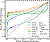 |
Fig. 5. Different combinations of baselines and periodicity shape (ROC curves). The solid lines show sinusoidal light curves, and the dashed lines show sawtooth light curves. The blue lines show the PTF-like baseline, orange lines show the idealised baseline, and green lines show the LSST baseline. The circles and squares identify the points at the identified Bayes threshold for the sinusoidal and sawtooth cases, respectively. The blue markers show PTF-like light curves, orange markers show ideal light curves and finally, green markers show LSST-like light curves. |
3.2. Recovery fractions and parameter recovery
The true- and false-positive fractions obtained using the ROC-based thresholds for each baseline and variability shape are summarised in Table 1.
Fractions of retrieved periodicities using the thresholds from the ROC curves.
From our analysis, we found that the true-positive fractions are similar for the sinusoidal and sawtooth scenarios for an idealised baseline of ∼68%. The efficiency of our algorithm decreases as the number of observational data points drops. Specifically, only ≈53% (≈26%) of the PTF-like light curves were identified as periodic in the sinusoidal (sawtooth) case. We interpret the stronger impact of fewer and sparser data on the sawtooth light curves as a consequence of their strong dependence on whether the fast-rising phase (the key signature distinguishing them from red noise) is included in the observations or lost in the gaps7.
Finally, the retrieved fractions for the LSST-like light curves are closer to those of the idealised case. They are slightly reduced at 59% for the sinusoidal scenario, regardless of the presence of quasi-periodic observational gaps and of the LSST-like light curves being a subset of PTF-like ones, for which the periodic model was not favoured over the noise-only model. As expected, an overall trend is that by increasing the number of data points or the number of observed cycles, the fraction of retrieved periodicities increases. We discuss the most relevant parameters for a correct identification of a periodic component in Section 3.4.
While our true-positive fraction is much larger than those quoted by alternative searches in the literature (e.g. Lin et al. 2026), we stress that it was not obtained by fixing a Bayes factor threshold, as we did in our ROC curve analysis. In Section 3.5 we determine a Bayes factor threshold to perform a fair comparison with the work by Lin et al. (2026) and show the change in the fraction of retrieved periodicities with that threshold.
As in Lin et al. (2026), we assessed the goodness of the parameter recovery using the relative fractional error on the period as a metric. In particular, we defined the metric of our test as
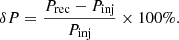 (9)
(9)
In Figure 6 we show the absolute value of the relative percent error (|δP|) versus the Bayes factor as a scatter plot. In particular, the relative error tends to decrease as the Bayes factor increases. In Table 2 we show the fraction of light curves containing a periodic signal that are correctly identified as periodic, and that show a retrieved period within 15% of the injected one for the three baselines and the two shapes of the modulation considered here.
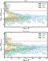 |
Fig. 6. Absolute value of the relative period recovery error as a function of the base-10 logarithm Bayes factor, shown as density contours at the 25th and 75th percentile levels obtained through Gaussian kernel density estimation. The blue, orange, and green markers show the ideal, PTF and LSST baselines, respectively. The horizontal dashed red line shows a reference value |δP| = 0.15. The upper panel shows sinusoidal light curves, and the lower panel shows sawtooth light curves. |
Fraction of retrieved periodicities with |δP|< 0.15 using the thresholds from the ROC curves.
The periods are well retrieved in the idealised and LSST cases for light curves with Bayes factors greater than the thresholds found through the ROC curves shown in Figure 5. The test does not recover the correct period in the PTF light curves as well as for the other baselines. This is mostly due to the sampling sparseness. A particularly interesting case is that of light curves exhibiting a sawtooth periodicity. As shown by the orange diamonds in Figure 6, a horizontal feature appears at |δP| = 1. This occurs because in these light curves, the sharp rise in the periodic signal is not observed in every cycle. The absence of this part of the signal causes the algorithm to identify a period that is twice the injected period.
3.3. Comparison with the cosine kernel
Similar periodicity searches using nested samplers to explore the parameter space of Gaussian processes have been performed in the literature (see Foustoul et al. 2025, for example), but, as mentioned in Section 1, we employed the cosine kernel as defined in Equation (7). Because of the different number of free parameters, the distribution of the false-positive fraction as a function of the assumed threshold on the Bayes factor is expected to be different. To study it, we analysed the same light curves as were used to build the distribution for the periodic kernel with the cosine kernel.
For the cosine kernel, the log10B thresholds found through the ROC curves, shown in Figure 7, are 1.29, 1.22, 1.06, and 0.86 for the ideal sinusoidal, ideal sawtooth, PTF ideal, and PTF sawtooth, respectively. The percentages of true- and false-positives found with the cosine kernel using these thresholds are summarised in the lower half of Table 1.
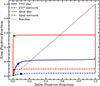 |
Fig. 7. Different combinations of baselines and periodicity shape found using the cosine kernel (ROC curves). The solid lines show sinusoidal light curves, and the dashed lines show sawtooth light curves. The blue lines show the PTF-like baseline, and the red lines show the idealised baseline. The circles and squares identify the points at the identified Bayes threshold for the sinusoidal and sawtooth cases, respectively. The blue markers show PTF-like light curves, and red markers show ideal light curves. |
The cosine kernel fails to determine periodicities that are not sinusoidal. In particular, for non-sinusoidal signals with sparse sampling, the fraction of false-positives at the identified threshold is much higher than the true-positive fraction. This is confirmed in Figure 8, where the ability of the cosine kernel to identify non-sinusoidal signals drops rapidly when compared to the generic periodic kernel.
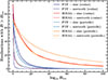 |
Fig. 8. Comparison of the fraction of realisations with a Bayes factor greater than a threshold as a function of the assumed threshold found using the cosine or generic periodic kernels. Dark blue and red lines show the results obtained with the cosine kernel for the PTF and ideal baselines, respectively. Blue and orange lines show the results obtained with the generic periodic kernel for the PTF and ideal baselines, respectively. Solid lines refer to sinusoidal modulations while dashed lines refers to sawtooth modulations. |
In Table 1, the cosine kernel also retrieves a lower fraction of true-positives in the idealised and sinusoidal scenario with respect to the fractions retrieved by the generic periodic kernel. This is mainly due to the different Bayes factor thresholds caused by the different shapes of the ROC curves. Figure 8 shows that in the comparison of the distributions of true-positives computed by using the periodic and cosine kernels, the fraction of true-positives for the cosine kernel is slightly larger than the one found through the generic periodic kernel because there are fewer parameters. On the other hand, the cosine kernel misses most of the sawtooth light curves for idealised and PTF-like baselines. For both kernels, the retrieved fractions for the idealised case are greater than those for the PTF-like light curves because the sampling of the latter is sparser.
3.4. Parameter importance
To identify the parameters that dominate the GP capability to identify periodicities, we performed a random forest regression (RFR, see Breiman 2001). RFR is an ensemble method able to perform regression on non-linear problems by combining the results from different decision trees, that is, a machine-learning algorithm where data are recursively split into smaller groups depending on feature (input variable) values. Each decision tree was trained using a subset of the input data and considered only a subset of the available features to introduce diversity among trees and reduce correlation. RFR is particularly useful as it allowed us to gauge the feature that affects the goodness of model predictions by the so-called feature importance (see Genuer et al. 2010). In particular, to assess the feature importance, we used the permutation feature importance: a measure of how much each feature contributes to a certain classification. This was obtained by determining how much the model accuracy drops when feature values are randomly shuffled. When a feature is important, its shuffling leads to a large drop in the predictive performance.
The feature importance of the periodic signal parameters and those of the DRW process are summarised in Table 3.
Feature importance.
The number of observed cycles Ncycles = Tobs/P is the parameter that affects the test ability to identify periodic signals most: the higher the number of observed cycles, the better the identification of periodicities by the test. The periodic signal and noise amplitudes (A and σ, respectively) have a relatively smaller impact on the periodicity identification. This is shown in Figure 9, where the light curves with a higher Bayes factor are also those with the higher number of cycles. Figure 9 also shows that light curves yielding high B tend to be found at higher S/N, with some scattering at lower S/N as well. This behaviour is expected as the amplitude has the highest feature importance after the period and length of the light curve.
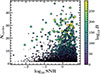 |
Fig. 9. Number of observed cycles plotted against S/N (A/σ), colour-coded by log10B. The marker size is proportional to log10B. |
3.5. Comparison with LSP-based searches
To define which light curves are correctly identified as periodic, Lin et al. (2026) generated 100 000 light curves with the same noise parameters and without periodicity for each of the 12 400 light curves analysed with injected periodicity. A light curve was considered periodic when its LSP showed at least one peak whose power exceeded that of all peaks found in the noise-only simulations. To compare our results with those found through the LSP analysis, we searched for the Bayes factor threshold with which we found one false positive every 105/25 light curves, where the factor 25 comes from the fact that they analysed 25 frequency bins at the same time. Since we sampled only 104 light curves for the combination of baselines taken into account in Figure 3, we used the fit shown as solid lines in the same figures to extrapolate the expected threshold for the LSST light curves, as we performed a preliminary analysis over ∼1000 light curves because of the computational cost. These values are shown in Figures 3 and 7 as vertical lines. For the comparison with the LSP analysis, we fixed a conservative Bayes factor threshold at log10Btrs = 5 for the PTF and ideal baselines and a threshold of log10Btrs = 3 for the LSST baselines. We note that these thresholds are much more conservative than those obtained from the ROC curves, mainly because we imposed a much lower FAP in this case.
The results obtained assuming the thresholds described above are summarised in Table 4. In the idealised case, our analysis correctly identified about 53% of the injected sinusoidal periodicities, 25% more than those identified through the LSP analysis by Lin et al. (2026)8. The difference is due to the nature of the algorithm, as the test statistic for periodicity detection (i.e. the Bayes factor) explicitly includes the red noise (see Robnik et al. 2024), while in Lin et al. 2026, the test statistic was the periodogram peak for which the underlying assumption was white noise.
Fractions of retrieved periodicities using the thresholds from the LSP FAP.
In the idealised sawtooth case, the difference is much more pronounced. It recovered more than half of the periodicities, while Lin et al. (2026) only identified about 1% of them. While the LSP analysis significantly underperforms when searching for non-sinusoidal signals, our analysis retrieved more sawtooth than sinusoidal signals, probably because the DRW has only one characteristic timescale, and it can either mimic the long-term variability associated with the period of the sawtooth signal or the sharp rise occurring at the beginning of each brightening, but never both. The appearance of long-term periodicities with sharp features limits the evidence of the DRW (noise-only) model, explaining the high true-positive rate of our search on the idealised sawtooth light curves.
As discussed in Section 3.2, the efficiency of our algorithm decreases as the number of observational data points drops. Assuming a log(Bthrs) = 5, only ≈23% (≈9%) of PTF-like light curves are identified as periodic in the sinusoidal (sawtooth) case.
The LSP analysis discussed in Lin et al. (2026) is apparently not affected by the lower number of data points and the observational gaps of about a month. It improves their detection fraction to ∼39% for the PTF-like sinusoidal light curves with respect to their idealised counterparts, which show a detection fraction of ∼28%. An even larger improvement (increasing from ∼1% in the idealised baseline to ∼7% in the PTF-like baseline) is observed in the light curves with a sawtooth periodicity. This increase in the LSP efficiency for sparser data is somewhat surprising (an opinion expressed in Lin et al. 2026, as well; see their discussion section) and might be associated with a lower degree of power leakage to frequencies associated with the one of the even sampling (see Lin et al. 2026 for more details).
When the Bayes factor threshold is fixed to log10Btrs = 5 for the idealised and PTF baselines or log10Btrs = 3 for the LSST baseline, the accuracy of the period recovery improves. The fraction of light curves showing a retrieved period within 15% of the injected one among all the light curves with a Bayes factor greater than the threshold for all the combinations of baselines and periodicity shapes is summarised in Table 5.
Fraction of light curves with a retrieved period within 15% of the injected one using the thresholds from the LSP FAP.
Finally, in Figure 10, we report the fraction of retrieved periodic signals as a function of the parameters as reported by Lin et al. (2026), where instead of the period, we plot the number of cycles, as we identified it as the most important parameter for our analysis (see Section 3.4). To do this, we divided the range of the injected S/N (A/σ), amplitude (A) and the number of observed cycles (Ncycles) into ten bins and computed the fraction of retrieved periodic light curves among all the light curves in each bin. As expected from the previous discussion, the fraction of retrieved light curves decreases as the period of the signal increases.
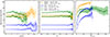 |
Fig. 10. Fraction of retrieved periodicities as a function of S/N, periodic signal amplitude (A), and number of observed cycles (Ncycles), shown from left to right. The shaded regions show the uncertainties on the points. |
4. Discussion and conclusions
We proposed a Bayesian framework based on GPs to identify arbitrarily shaped periodicities in evenly and unevenly sampled light curves. The method leverages Gaussian processes to model the periodic and stochastic variability and nested sampling to determine the relative evidence of a periodicity in the data and to constrain the associated periods.
We studied the performance of the method characterising the fractions of true-positives (periodic signals correctly identified as periodic) and false-positives (realisations of standard AGN variability misidentified as periodic signals) as a function of the Bayes factor B, defined as the ratio of the evidence of a model including a periodic component and a model with non-periodic variability alone. An optimal threshold Btrs was identified for each type of light curve (characterised by the duration of the monitoring campaign Tobs and the frequency and regularity of the observations) to maximise the fraction of true-positive detections while limiting the contamination by false-positives. With this threshold, the percentages of true-positives are as high as ≈70% for idealised baselines (even sampling every day with durations extracted from real PTF light curves) regardless of the periodicity shape, and decrease to ≈53% (≈26%) for sinusoidal (sawtooth) periodicities sampled with the same Tobs as the idealised ones and with uneven sampling of real PTF data (PTF baseline). The decreased efficiency of the algorithm for sparser data and sawtooth-shaped signals is associated with the possibility that the rapid rise in the luminosity can fall in data gaps, hindering the correct identification of periodicities. For the same reason, while in the other cases > 80% of the retrieved periods are accurate within a relative error of 15%, the PTF baselines recover the incorrect period in up to ∼40% of the light curves identified as periodic. In all the considered scenarios, the false-alarm probability was < 15%9.
The generic periodic GP kernel we adopted is more versatile than the cosine kernel previously used in literature for the analysis of AGN light curves (Zhu & Thrane 2020; Foustoul et al. 2025): while the cosine kernel performs similarly, for sinusoidal signals, it recovers < 6% of the sawtooth periodicities even after the optimisation of Btrs. This low fraction of true-positives is expected because the cosine kernel struggles to simultaneously model the correct period and sharp features in the light curves.
We completed our comparison study by comparing the performances of our model with the study by Lin et al. (2026) based on Lomb-Scargle-periodogram analyses. These searches identify periodic signals on the basis of a false-alarm threshold. We therefore identified a conservative threshold to be used to perform a fair comparison with the results presented in Lin et al. (2026) at log10B = 5 for idealised and PTF-like light curves and log10B = 3 for LSST-like light curves. With this new (significantly higher) threshold, the fraction of identified modulations in idealised sinusoidal light curves decreased to ∼53%, which is higher than the ∼28% obtained using the LSP-analysis. Even more relevant is the increase in recovered periodicities in the idealised sawtooth case, with more than 58% of the systems being identified compared to the ∼1% recoveries in Lin et al. (2026). As for the ROC-optimised Btrs, even assuming log10Btrs = 5, we found that periodicities in PTF-like light curves were retrieved in a much smaller fraction than in the idealised case because of their sparse sampling. Surprisingly, no such trend was observed by Lin et al. (2026), who found a significant increase (up to a factor of ≈7 for sawtooth light curves) in the recovery fraction with fewer and sparser data with quasi-periodic gaps. A more detailed comparison to clarify the reason for this behaviour is deferred to a future investigation.
The main feature determining the recovery fraction of periodic signals in our model is the number of periods in the light curves. To gauge the performance of our method for longer surveys and to test its relevance for the starting LSST campaign, we selected the properties (of the periodic component and of the noise) of 1000 light curves that were not identified with PTF baselines and resampled them with LSST-like baselines. Of these 1000, about 60% (70%) light curves were correctly identified as periodic with a small fraction of false-positives and about ∼2% (3%) in the sinusoidal (sawtooth) case.
The ability to identify non-sinusoidal shapes of periodic signals is of fundamental importance for the search for MBHBs. Sawtooth-like light curves are expected when the periodicity is imprinted by the periodic feeding of the two massive black hole mini discs (caused by the periodic non-axisymmetric potential of the binary). Deviations from sinusoidal modulations are also expected for periodicities caused by periodic gravitational lensing involving an MBHB or by Doppler boosting in an eccentric binary, even in the idealised scenario of constant intrinsic luminosity.
In principle, our analysis can be tailored for the identification of non-active MBHB when a luminous star in the binary host galaxy is periodically lensed by the two MBHs (Wang et al. 2026), and it can be used for astrophysical systems other than MBHBs, such as quasi-periodic eruptions (QPE, see Miniutti et al. 2019; Giustini et al. 2020; Arcodia et al. 2021), which are high-amplitude bursts of X-ray radiation that recur every few hours and originate near the central supermassive black holes of galactic nuclei, or even planetary transits that are used for the search of exoplanets by determining periodic dips in the flux of a star (see Holman & Murray 2005; Winn et al. 2010). In Appendix B we demonstrate that the test can also retrieve the correct periodicities for sharp and narrow periodic modulations in the light curves, as expected in the examples above. In this case, we find that, unlike in the sinusoidal and sawtooth cases, the signal-to-noise ratio plays a crucial role in the detection of periodicities because, for spiky periodicities, most of the signal is concentrated within narrow time windows and is completely absent outside them. As a result, our analysis can no longer reliably distinguish the periodic component from the noise when the noise amplitude becomes comparable to that of the spiky signal.
In Appendix C, we compare the computational cost of the algorithm of this work with that of the Lomb-Scargle analysis as implemented in Charisi et al. (2016), showing that the algorithm presented here is more computationally expensive. We stress that, along with this additional computational cost, comes the advantage of a full Bayesian framework. This provides posterior distributions on the model parameters and allows us to robustly compare the model via Bayesian evidence, which is not available with the Lomb-Scargle periodogram.
To improve our search strategy, it is essential to simultaneously leverage photometric points collected in multiple bands. We plan to do so using multi-output Gaussian processes to allow us to analyse all the available bands in parallel so that they can inform one another. This procedure has a high computational cost because the numerical burden scales approximately as the cube of the number of observations10 in all the bands. This is a major limitation of our method, which is still too slow to be applied to the entire LSST quasar sample. For this reason, we are working on the parallelisation of our algorithm on GPUs.
This method can be further generalised by considering other noise models, for instance the damped harmonic oscillator (DHO, see Yu et al. 2022). We did not perform this analysis in this first exploratory work because the light curves we used to compare our performances with alternative searches were generated assuming the DRW as the noise model. The characterisation of the performances of our search for different noise models is deferred to a future investigation.
Acknowledgments
LB acknowledges ISCRA for awarding this project access to the LEONARDO supercomputer, owned by the EuroHPC Joint Undertaking, hosted by CINECA (Italy). LB wishes to thank the “Summer School for Astrostatistics in Crete” for providing training on the statistical methods adopted in this work. MD and RB acknowledge support from the ICSC National Research Center funded by NextGenerationEU, and financial support by the Italian Space Agency grant Phase B2/C activity for LISA mission, Agreement n.2024-NAZ-0102/PE. MC is funded by the European Union (ERC-StG-2023, MMMonsters, 101117624). JCR acknowledges support from the National Science Foundation (NSF) from grant NSF AST-2205719 and the NASA Preparatory Science program under award 20-LPS20-0013.
References
- Agazie, G., Anumarlapudi, A., Archibald, A. M., et al. 2023, ApJ, 951, L8 [NASA ADS] [CrossRef] [Google Scholar]
- Aigrain, S., & Foreman-Mackey, D. 2022, arXiv e-prints [arXiv:2209.08940] [Google Scholar]
- Amaro-Seoane, P., Audley, H., & Babak, S. 2017, ArXiv e-prints [arXiv:1702.00786] [Google Scholar]
- Amaro-Seoane, P., Andrews, J., Arca Sedda, M., et al. 2023, Liv. Rev. Relativ., 26, 2 [NASA ADS] [CrossRef] [Google Scholar]
- Angus, R., Morton, T., Aigrain, S., Foreman-Mackey, D., & Rajpaul, V. 2018, MNRAS, 474, 2094 [Google Scholar]
- Arcodia, R., Merloni, A., Nandra, K., et al. 2021, Nature, 592, 704 [NASA ADS] [CrossRef] [Google Scholar]
- Begelman, M. C., Blandford, R. D., & Rees, M. J. 1980, Nature, 287, 307 [Google Scholar]
- Bertassi, L., Sottocorno, E., Rigamonti, F., et al. 2025, A&A, 702, A165 [NASA ADS] [CrossRef] [EDP Sciences] [Google Scholar]
- Bogdanović, T., Miller, M. C., & Blecha, L. 2022, Liv. Rev. Relativity, 25, 3 [Google Scholar]
- Bortolas, E., Capelo, P. R., Zana, T., et al. 2020, MNRAS, 498, 3601 [Google Scholar]
- Bortolas, E., Bonetti, M., Dotti, M., et al. 2022, MNRAS, 512, 3365 [NASA ADS] [CrossRef] [Google Scholar]
- Breiman, L. 2001, Mach. Learn., 45, 5 [Google Scholar]
- Chan, C.-H., Tiwari, V., Bogdanović, T., Jiang, Y.-F., & Davis, S. W. 2025, ApJ, 991, 71 [Google Scholar]
- Charisi, M., Bartos, I., Haiman, Z., et al. 2016, MNRAS, 463, 2145 [Google Scholar]
- Chen, Y.-C., Liu, X., Liao, W.-T., et al. 2020, MNRAS, 499, 2245 [Google Scholar]
- Chen, Y.-J., Zhai, S., Liu, J.-R., et al. 2024, MNRAS, 527, 12154 [Google Scholar]
- Cocchiararo, F., Franchini, A., Lupi, A., & Sesana, A. 2024, A&A, 691, A250 [NASA ADS] [CrossRef] [EDP Sciences] [Google Scholar]
- Covino, S., Landoni, M., Sandrinelli, A., & Treves, A. 2020, ApJ, 895, 122 [NASA ADS] [CrossRef] [Google Scholar]
- Covino, S., Tobar, F., & Treves, A. 2022, MNRAS, 513, 2841 [Google Scholar]
- De Rosa, A., Vignali, C., Bogdanović, T., et al. 2019, New Astron. Rev., 86, 101525 [Google Scholar]
- del Valle, L., Escala, A., Maureira-Fredes, C., et al. 2015, ApJ, 811, 59 [NASA ADS] [CrossRef] [Google Scholar]
- D’Orazio, D. J., & Charisi, M. 2023, ArXiv e-prints [arXiv:2310.16896]. [Google Scholar]
- D’Orazio, D. J., & Di Stefano, R. 2018, MNRAS, 474, 2975 [CrossRef] [Google Scholar]
- D’Orazio, D. J., Haiman, Z., & Schiminovich, D. 2015, Nature, 525, 351 [Google Scholar]
- Dotti, M., Sesana, A., & Decarli, R. 2012, Adv. Astron., 2012, 940568 [CrossRef] [Google Scholar]
- Dotti, M., Bonetti, M., D’Orazio, D. J., Haiman, Z., & Ho, L. C. 2022, MNRAS, 509, 212 [Google Scholar]
- Dotti, M., Rigamonti, F., Rinaldi, S., et al. 2023, A&A, 680, A69 [NASA ADS] [CrossRef] [EDP Sciences] [Google Scholar]
- Duffell, P. C., D’Orazio, D., Derdzinski, A., et al. 2020, ApJ, 901, 25 [NASA ADS] [CrossRef] [Google Scholar]
- Durrande, N., Hensman, J., Rattray, M., & Lawrence, N. D. 2016, arXiv e-prints [arXiv:1303.7090] [Google Scholar]
- El-Badry, K., Hogg, D. W., & Rix, H.-W. 2026, PASP, 138, 024102 [Google Scholar]
- EPTA Collaboration, InPTA Collaboration, Antoniadis, J., et al. 2023, A&A, 678, A50 [CrossRef] [EDP Sciences] [Google Scholar]
- Fernandes, G. G. D., Barroca, M. A., dos Santos, M., & Oliveira, R. S. 2025, arXiv e-prints [arXiv:2511.17564] [Google Scholar]
- Fiacconi, D., Mayer, L., Roškar, R., & Colpi, M. 2013, ApJ, 777, L14 [NASA ADS] [CrossRef] [Google Scholar]
- Foreman-Mackey, D., Agol, E., Ambikasaran, S., & Angus, R. 2017, AJ, 154, 220 [Google Scholar]
- Foustoul, V., Webb, N. A., Mignon-Risse, R., et al. 2025, A&A, 699, A55 [NASA ADS] [CrossRef] [EDP Sciences] [Google Scholar]
- Gardner, J. R., Pleiss, G., Bindel, D., Weinberger, K. Q., & Wilson, A. G. 2021, arXiv e-prints [arXiv:1809.11165] [Google Scholar]
- Gaskell, C. M. 1988, Active Galactic Nuclei, 307, 61 [Google Scholar]
- Genuer, R., Poggi, J.-M., & Tuleau-Malot, C. 2010, Pattern Recog. Lett., 31, 2225 [Google Scholar]
- Giustini, M., Miniutti, G., & Saxton, R. D. 2020, A&A, 636, L2 [NASA ADS] [CrossRef] [EDP Sciences] [Google Scholar]
- González-Álvarez, E., Petralia, A., Micela, G., et al. 2021, A&A, 649, A157 [NASA ADS] [CrossRef] [EDP Sciences] [Google Scholar]
- Graham, M. J., Djorgovski, S. G., Stern, D., et al. 2015, MNRAS, 453, 1562 [Google Scholar]
- Haiman, Z., Xin, C., Bogdanović, T., et al. 2023, ArXiv e-prints [arXiv:2306.14990] [Google Scholar]
- Hayasaki, K., Mineshige, S., & Ho, L. C. 2008, ApJ, 682, 1134 [NASA ADS] [CrossRef] [Google Scholar]
- Haywood, R. D., Collier Cameron, A., Queloz, D., et al. 2014, MNRAS, 443, 2517 [Google Scholar]
- Holman, M. J., & Murray, N. W. 2005, Science, 307, 1288 [Google Scholar]
- Hu, B. X., D’Orazio, D. J., Haiman, Z., et al. 2020, MNRAS, 495, 4061 [Google Scholar]
- Ivezić, Ž., Kahn, S. M., Tyson, J. A., et al. 2019, ApJ, 873, 111 [Google Scholar]
- Jeffreys, H. 1998, The Theory of Probability, Oxford Classic Texts in the Physical Sciences (OUP Oxford) [Google Scholar]
- Kelley, L. Z., Haiman, Z., Sesana, A., & Hernquist, L. 2019, MNRAS, 485, 1579 [NASA ADS] [CrossRef] [Google Scholar]
- Kelley, L. Z., D’Orazio, D. J., & Di Stefano, R. 2021, MNRAS, 508, 2524 [NASA ADS] [CrossRef] [Google Scholar]
- Kelly, B. C., Bechtold, J., & Siemiginowska, A. 2009, ApJ, 698, 895 [Google Scholar]
- Kormendy, J., & Gebhardt, K. 2001, Am. Inst. Phys. Conf. Ser., 586, 363 [Google Scholar]
- Kovačević, A. B., Ilić, D., Popović, L. Č., et al. 2023, Universe, 9, 287 [Google Scholar]
- Kozłowski, S., Kochanek, C. S., Stern, D., et al. 2010, ApJ, 716, 530 [CrossRef] [Google Scholar]
- Li, J., Wang, Z., & Zheng, D. 2023, MNRAS, 522, 2928 [NASA ADS] [CrossRef] [Google Scholar]
- Lin, A., Charisi, M., & Haiman, Z. 2026, ApJ, 997, 316 [Google Scholar]
- Liu, T., Gezari, S., Ayers, M., et al. 2019, ApJ, 884, 36 [Google Scholar]
- Lomb, N. R. 1976, Ap&SS, 39, 447 [Google Scholar]
- MacFadyen, A. I., & Milosavljević, M. 2008, ApJ, 672, 83 [Google Scholar]
- MacLeod, C. L., Ivezić, Ž., Kochanek, C. S., et al. 2010, ApJ, 721, 1014 [Google Scholar]
- Marcum, J. I. 1947, A Statistical Theory of Target Detection by Pulsed Radar (Santa Monica, CA: RAND Corporation) [Google Scholar]
- McLaughlin, S. A. J., Mullaney, J. R., & Littlefair, S. P. 2024, MNRAS, 529, 2877 [Google Scholar]
- Miller, N., Lucas, P. W., Sun, Y., et al. 2024, RAS Techn. Instrum., 3, 224 [Google Scholar]
- Miniutti, G., Saxton, R. D., Giustini, M., et al. 2019, Nature, 573, 381 [Google Scholar]
- Rasmussen, C. E., & Williams, C. K. I. 2006, Gaussian Processes for Machine Learning [Google Scholar]
- Reardon, D. J., Zic, A., Shannon, R. M., et al. 2023, ApJ, 951, L6 [NASA ADS] [CrossRef] [Google Scholar]
- Rigamonti, F., Bertassi, L., Buscicchio, R., et al. 2025, A&A, 702, A242 [NASA ADS] [CrossRef] [EDP Sciences] [Google Scholar]
- Robnik, J., Bayer, A. E., Charisi, M., et al. 2024, MNRAS, 534, 1609 [Google Scholar]
- Scargle, J. D. 1982, ApJ, 263, 835 [Google Scholar]
- Skilling, J. 2006, Bayesian Anal., 1, 833 [Google Scholar]
- Souza Lima, R., Mayer, L., Capelo, P. R., & Bellovary, J. M. 2017, ApJ, 838, 13 [NASA ADS] [CrossRef] [Google Scholar]
- Tubín-Arenas, D., Krumpe, M., Homan, D., et al. 2025, A&A, 698, A192 [NASA ADS] [CrossRef] [EDP Sciences] [Google Scholar]
- Ulrich, M.-H., Maraschi, L., & Urry, C. M. 1997, ARA&A, 35, 445 [NASA ADS] [CrossRef] [Google Scholar]
- Vanderburg, A., Montet, B. T., Johnson, J. A., et al. 2015, ApJ, 800, 59 [NASA ADS] [CrossRef] [Google Scholar]
- VanderPlas, J. T. 2018, ApJS, 236, 16 [Google Scholar]
- Vaughan, S., Uttley, P., Markowitz, A. G., et al. 2016, MNRAS, 461, 3145 [Google Scholar]
- Veitch, J., Del Pozzo, W., Lyttle, A., et al. 2024, A&A [Google Scholar]
- Verbiest, J. P. W., Lentati, L., Hobbs, G., et al. 2016, MNRAS, 458, 1267 [Google Scholar]
- Wang, M., Yuan, H., Bai, Z., et al. 2025, AJ, 170, 184 [Google Scholar]
- Wang, H., Zumalacárregui, M., & Kocsis, B. 2026, Phys. Rev. Lett., 136, 061403 [Google Scholar]
- Westernacher-Schneider, J. R., Zrake, J., MacFadyen, A., & Haiman, Z. 2022, Phys. Rev. D, 106, 103010 [NASA ADS] [CrossRef] [Google Scholar]
- Winn, J. N. 2010, in Exoplanets, ed. S. Seager, 55 [Google Scholar]
- Witt, C. A., Charisi, M., Taylor, S. R., & Burke-Spolaor, S. 2022, ApJ, 936, 89 [NASA ADS] [CrossRef] [Google Scholar]
- Xin, C., & Haiman, Z. 2021, MNRAS, 506, 2408 [NASA ADS] [CrossRef] [Google Scholar]
- Xu, H., Chen, S., Guo, Y., et al. 2023, Res. Astron. Astrophys., 23, 075024 [CrossRef] [Google Scholar]
- Yu, W., Richards, G. T., Vogeley, M. S., Moreno, J., & Graham, M. J. 2022, ApJ, 936, 132 [NASA ADS] [CrossRef] [Google Scholar]
- Yu, W., Ruan, J. J., Burke, C. J., et al. 2026, ApJ, 998, 144 [Google Scholar]
- Zhang, H., Yan, D., & Zhang, L. 2023, ApJ, 944, 103 [Google Scholar]
- Zhang, H., Yang, S., & Dai, B. 2024, ApJ, 967, L18 [Google Scholar]
- Zhu, X.-J., & Thrane, E. 2020, ApJ, 900, 117 [NASA ADS] [CrossRef] [Google Scholar]
- Zrake, J., Tiede, C., MacFadyen, A., & Haiman, Z. 2021, ApJ, 909, L13 [NASA ADS] [CrossRef] [Google Scholar]
The list of physical processes imprinting a periodicity on the observed light curve is not definitely complete, as other processes might contribute to a periodic modulation (see e.g. Chan et al. 2025).
Uneven sampling and gaps in the observations of individual objects are unavoidable, due to weather interruptions, sources falling below the horizon or very close to the Sun during certain seasons. Space-based observatories achieve more regular coverage, but still experience interruptions due to operational constraints.
From a statistical point of view, the log-likelihood in Eq. (3) is in fact the marginal one for a single GP model, while Z is the (hyper-)evidence of each chosen GP family, e.g. the three specified in Sects. 2.1, 2.2, and 2.3. We opted for a slight misnaming as it is ubiquitous in relevant literature.
We note that rescaling the time axis by the standard deviation of the observation times is effectively similar to rescaling by the total duration of the light curve. This normalisation prevented us from exploring timescales that are much longer than the observed baseline.
The multiplicative factor 25 comes from the fact that when analysing the LSP, Lin et al. (2026) used 25 frequency bins.
This can be demonstrated by considering a point (FP0, TP0) and the one-to-one line TP = FP. The distance between the point and the line is given by  . Maximising this distance implies d(TP − FP)/dFP = 0, and thus, dTP/dFP = 1.
This occurrence is rarer the longer the light curve because it is unlikely that all peaks fall in gaps. The analysis of LSST-like data presented below further supports this interpretation.
To obtain the same detection fraction, we would need to raise our detection threshold to log(Btrs) = 18.12.
After it is selected, the FAP of each light curve can be individually evaluated from its value of B.
We note that the effective computational cost of the likelihood evaluation, which dominates the computational burden of the algorithm, strongly depends on the implementation and on the type of covariance matrix assumed. Examples of different scalings are GpyTorch (see Gardner et al. 2021, and Appendix C) and celerite (see Foreman-Mackey et al. 2017).
Appendix A: The periodic kernel
In Section 2.3, we briefly discussed how the periodic kernel is defined and how it describes signals with arbitrary shapes thanks to the presence of a kernel length scale. In the top panel of Figure A.1, we show how realisations of the Gaussian process change when changing the kernel length scale. In the bottom panel, we show, for visualisation purposes, the rescaled periodic kernel defined as
 (A.1)
(A.1)
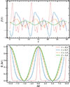 |
Fig. A.1. Upper panel: realisations of a Gaussian process with a periodic kernel at different length scales. Lower panel: rescaled periodic kernel |

where Δt = |ti − tj| with ti, tj being two observations of the timeseries. Note that changes when changing its length scale. From Figure A.1, it is possible to see that, as the length scale decreases, only observations that are very close in time or separated by an integer multiple of the period remain strongly correlated, while the correlation drops rapidly for points in between these peaks, allowing for the modelling of sharp features in the light curves.
The flexibility of the periodic kernel can also be explained by means of the Fourier-Bessel expansion. The periodic kernel can be rewritten as:
![Mathematical equation: $$ \begin{aligned} k_{\mathrm{periodic}}(t_i, t_j) = A^2 \exp \left(-\frac{1}{l^2}\right) \exp \left[\frac{1}{l^2}\cos \left(\frac{2\pi }{P} | t_i - t_j | \right)\right] . \end{aligned} $$](/articles/aa/full_html/2026/07/aa58583-25/aa58583-25-eq16.gif) (A.2)
(A.2)
By recalling that exp[acos(θ)] can be expanded as:
![Mathematical equation: $$ \begin{aligned} \exp [a\cos (\theta )] = I_0(a) + 2\sum _{n = 1}^\infty I_n(a) \cos (n\theta ), \end{aligned} $$](/articles/aa/full_html/2026/07/aa58583-25/aa58583-25-eq17.gif) (A.3)
(A.3)
where In are the modified Bessel functions, we get:
![Mathematical equation: $$ \begin{aligned} \begin{split} k_{\rm periodic}(t_i, t_j)&= A^2 \exp \left(-\frac{1}{l^2}\right) \Bigg [ I_0\left(\frac{1}{l^2}\right) \\&+ 2\sum _{n = 1}^\infty I_n\left(\frac{1}{l^2}\right) \cos \left(\frac{2\pi n}{P} |t_i - t_j|\right) \Bigg ]. \end{split} \end{aligned} $$](/articles/aa/full_html/2026/07/aa58583-25/aa58583-25-eq18.gif) (A.4)
(A.4)
From this expansion, it becomes clear that the kernel describes an infinite series of Fourier modes with weights exp(−1/l2)In(1/l2). As l2 → ∞, the only significant term is the n = 1 harmonic as the Bessel weights In(1/l2) vanish for n > 1 when the argument is small, while for l2 → 0, many harmonics contribute to the signal. Such an expansion shows that, similarly to the Lomb–Scargle periodogram, the periodic kernel represents a periodic signal as a decomposition into harmonics. However, instead of explicitly fitting independent amplitudes for each Fourier mode, the relative weighting of the harmonics is implicitly controlled by the kernel length scale. This allows the periodicity search algorithm to self-consistently leverage the power at different harmonics, resulting in a higher retrieved fraction compared to the LSP-based algorithm searching for an excess of signal at only one frequency.
Appendix B: Searching for spiky signals
As briefly mentioned in Section 1, in both cases of active or dormant massive black holes, depending on the inclination of the system, "spiky" signals are expected because of gravitational lensing, either the lensing of one massive black hole on its companion or because of the lensing of the MBHB onto a background star (see Wang et al. 2026). Similarly to the case of sawtooth signals, when computing the periodogram, the power leaks to frequencies different from the inverse of the true period. Thus, the LSP analysis would encounter the same problems as in the sawtooth case, while the GP analysis would also be able to detect this kind of signal. In Figure B.1, we show that, in the absence of red noise and with an idealised baseline characterised by an even sampling and a cadence sufficient to resolve the sudden rise and fall of the flux (the light curve is sampled 4 times per day in this case), the GP analysis can successfully identify both the shape and period of spiky signals when using the periodic kernel. Similarly to the sawtooth case in Figure 1, the cosine kernel is unable to properly describe the shape of the spiky signal. For the light curve shown in Figure B.1, the Bayes factor between the periodic and cosine kernel is log10Eperiodic/Ecosine ∼ 300. When windows in the sampling are introduced, the GP test begins to struggle and starts to identify longer periods in addition to the true one. This effect can be seen in Figure B.2, where one can see that multimodalities in the retrieved period are introduced due to the windowing. Also in this case, though, the cosine kernel seems unable to describe the spiky nature of the signal, with the periodic kernel being favoured with a Bayes factor of log10Eperiodic/Ecosine ∼ 200.
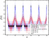 |
Fig. B.1. Posterior predictive distributions obtained by fitting a "spiky" light curve using the cosine kernel (red solid line and shaded region) and periodic kernel (blue solid line and shaded region) defined in Equations 7 and 8, respectively. The light curve is sampled 4 times per day. Similarly to the sawtooth case in Figure 1, the cosine kernel is unable to properly describe the shape of the periodic signal, while the periodic kernel manages to capture it. The time t and signal f(t) are reported in arbitrary units. |
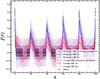 |
Fig. B.2. Posterior predictive distributions obtained by fitting a "spiky" light curve using the cosine kernel (red solid line and shaded region) and periodic kernel (blue solid line and shaded region) defined in Equations 7 and 8, respectively. The light curve is made sparser with respect to the light curve shown in Figure B.1 by the introduction of gaps in the data. The time t and signal f(t) are reported in arbitrary units. |
We repeated the same study done for the sinusoidal and sawtooth light curves for 3000 evenly sampled spiky light curves, finding that 42.53% of the periodicities are detected. The main difference from the previous results is that spiky light curves show a strong dependence on the signal-to-noise ratio, as shown in Figure B.3. This arises because the periodic signal is only visible for a very brief fraction of the observation; during the rest of the time, the light curve is dominated by noise. Consequently, when the noise amplitude becomes comparable to that of the periodic signal, the signal is effectively lost, unlike the sinusoidal or sawtooth cases, where the signal is present more continuously.
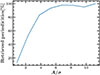 |
Fig. B.3. Fraction of retrieved periodicities as a function of signal-to-noise ratio (S/N) |
Appendix C: Computational cost comparison
As mentioned throughout this paper, the algorithm we propose, which leverages Gaussian and nested sampling, scales very differently compared to the more common Lomb-Scargle periodogram analysis. The latter algorithm, as implemented by Charisi et al. (2016) and Lin et al. (2026), with which we are comparing our results, is dominated by the generation of DRW light curves to assess the probability for a peak observed in the real light curve to be explained by pure-noise realisations. The algorithm presented in this work is instead dominated by the number of likelihood evaluations necessary for the nested sampler to converge, and the computational cost of each likelihood evaluation.
In Figure C.1, we show the very different scaling of the computational times of the two algorithms. We fitted the times to assess the scaling with the number of points, observing that the Lomb-Scargle analysis scales roughly linearly with the number of points, while the algorithm presented in this work scales roughly as N2, where N is the number of points in the light curve. We notice that the computational cost, measured as end-to-end runtimes, does not scale as the computational cost of a GP with an N × N covariance matrix. This is due to the way in which the likelihood is evaluated by GPyTorch, which uses a batched version of linear conjugate gradients (see Gardner et al. 2021) instead of a Cholesky decomposition. This reduces the time complexity of exact GP likelihood evaluation from O(N3) to O(N2). We also note that the total runtime captures any variation in the number of likelihood evaluations required by the nested sampler to reach convergence, which may itself depend on the complexity of the posterior and the data quality. The light curves used to evaluate the computational cost are idealised, and both the Lomb-Scargle and GP analyses have been run with no further parallelisation.
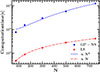 |
Fig. C.1. Comparison between the computational cost in seconds as a function of the number of points in an idealised light curve for the algorithm proposed in this work (blue points) and the Lomb-Scargle analysis as implemented in Charisi et al. (2016) (red points). The blue and red dashed lines show a power law fit to the data. |
All Tables
Fraction of retrieved periodicities with |δP|< 0.15 using the thresholds from the ROC curves.
Fraction of light curves with a retrieved period within 15% of the injected one using the thresholds from the LSP FAP.
All Figures
|
Fig. 1. Posterior predictive distributions from GP inference on a sinusoidal light curve (upper panel) and a sawtooth light curve (lower panel). The results from the cosine kernel (Equation 7) are shown in red, and those from the periodic kernel (Equation 8) are plotted in blue. The shaded regions indicate the 1σ (dark) and 2σ (light) credible intervals. |
| In the text | |
|
Fig. 2. Examples of the same sampled sinusoidal light curve for the three baselines. The LSST light curve is shown in the main panel, and the PTF (blue points) and ideal (orange points) light curves are displayed in the inset (lower right). The dashed red rectangle in the main panel highlights the typical duration of the PTF and ideal sampling, emphasising the longer observational coverage of the LSST baseline. |
| In the text | |
|
Fig. 3. Distribution of the Bayes factors for the 104 noise-only light curves for the PTF using the periodic kernel and cosine kernel (blue and dark blue distributions) and ideal using the periodic kernel and cosine kernel (orange and red distributions) baselines, and the 103 noise-only light curves for the LSST (green distribution) baseline found by analysing the light curves with the generic periodic kernel. The vertical lines refer to the Bayes factor threshold identified for a fair comparison with the LSP analysis discussed in more detail in Section 3.5. |
| In the text | |
|
Fig. 4. Fraction of the realisation containing periodic signals with a Bayes factor greater than a threshold as a function of the assumed threshold. The solid lines show the sinusoidal light curves, and the dotted lines show sawtooth light curves. Orange, blue and green show the ideal, PTF, and LSST baselines, respectively. The vertical lines show the Bayes factor threshold of log10Btrs = 5 for the ideal, PTF (solid line), and log10Btrs = 3 for the LSST baseline (dashed line) used to compare the results with the LSP analysis (see Section 3.5). The circles and squares identify the points at the identified ROC curve-based Bayes threshold for the sinusoidal and sawtooth cases, respectively. The orange markers show ideal-like light curves, blue markers show PTF-like light curves, and finally, green markers show LSST-like light curves. |
| In the text | |
|
Fig. 5. Different combinations of baselines and periodicity shape (ROC curves). The solid lines show sinusoidal light curves, and the dashed lines show sawtooth light curves. The blue lines show the PTF-like baseline, orange lines show the idealised baseline, and green lines show the LSST baseline. The circles and squares identify the points at the identified Bayes threshold for the sinusoidal and sawtooth cases, respectively. The blue markers show PTF-like light curves, orange markers show ideal light curves and finally, green markers show LSST-like light curves. |
| In the text | |
|
Fig. 6. Absolute value of the relative period recovery error as a function of the base-10 logarithm Bayes factor, shown as density contours at the 25th and 75th percentile levels obtained through Gaussian kernel density estimation. The blue, orange, and green markers show the ideal, PTF and LSST baselines, respectively. The horizontal dashed red line shows a reference value |δP| = 0.15. The upper panel shows sinusoidal light curves, and the lower panel shows sawtooth light curves. |
| In the text | |
|
Fig. 7. Different combinations of baselines and periodicity shape found using the cosine kernel (ROC curves). The solid lines show sinusoidal light curves, and the dashed lines show sawtooth light curves. The blue lines show the PTF-like baseline, and the red lines show the idealised baseline. The circles and squares identify the points at the identified Bayes threshold for the sinusoidal and sawtooth cases, respectively. The blue markers show PTF-like light curves, and red markers show ideal light curves. |
| In the text | |
|
Fig. 8. Comparison of the fraction of realisations with a Bayes factor greater than a threshold as a function of the assumed threshold found using the cosine or generic periodic kernels. Dark blue and red lines show the results obtained with the cosine kernel for the PTF and ideal baselines, respectively. Blue and orange lines show the results obtained with the generic periodic kernel for the PTF and ideal baselines, respectively. Solid lines refer to sinusoidal modulations while dashed lines refers to sawtooth modulations. |
| In the text | |
|
Fig. 9. Number of observed cycles plotted against S/N (A/σ), colour-coded by log10B. The marker size is proportional to log10B. |
| In the text | |
|
Fig. 10. Fraction of retrieved periodicities as a function of S/N, periodic signal amplitude (A), and number of observed cycles (Ncycles), shown from left to right. The shaded regions show the uncertainties on the points. |
| In the text | |
|
Fig. A.1. Upper panel: realisations of a Gaussian process with a periodic kernel at different length scales. Lower panel: rescaled periodic kernel |
| In the text | |
|
Fig. B.1. Posterior predictive distributions obtained by fitting a "spiky" light curve using the cosine kernel (red solid line and shaded region) and periodic kernel (blue solid line and shaded region) defined in Equations 7 and 8, respectively. The light curve is sampled 4 times per day. Similarly to the sawtooth case in Figure 1, the cosine kernel is unable to properly describe the shape of the periodic signal, while the periodic kernel manages to capture it. The time t and signal f(t) are reported in arbitrary units. |
| In the text | |
|
Fig. B.2. Posterior predictive distributions obtained by fitting a "spiky" light curve using the cosine kernel (red solid line and shaded region) and periodic kernel (blue solid line and shaded region) defined in Equations 7 and 8, respectively. The light curve is made sparser with respect to the light curve shown in Figure B.1 by the introduction of gaps in the data. The time t and signal f(t) are reported in arbitrary units. |
| In the text | |
|
Fig. B.3. Fraction of retrieved periodicities as a function of signal-to-noise ratio (S/N) |
| In the text | |
|
Fig. C.1. Comparison between the computational cost in seconds as a function of the number of points in an idealised light curve for the algorithm proposed in this work (blue points) and the Lomb-Scargle analysis as implemented in Charisi et al. (2016) (red points). The blue and red dashed lines show a power law fit to the data. |
| In the text | |
Current usage metrics show cumulative count of Article Views (full-text article views including HTML views, PDF and ePub downloads, according to the available data) and Abstracts Views on Vision4Press platform.
Data correspond to usage on the plateform after 2015. The current usage metrics is available 48-96 hours after online publication and is updated daily on week days.
Initial download of the metrics may take a while.