| Issue |
A&A
Volume 699, July 2025
|
|
|---|---|---|
| Article Number | A55 | |
| Number of page(s) | 19 | |
| Section | The Sun and the Heliosphere | |
| DOI | https://doi.org/10.1051/0004-6361/202452818 | |
| Published online | 30 June 2025 | |
A catalogue of candidate milliparsec-separation massive black hole binaries from long-term optical photometric monitoring
1
IRAP, Université de Toulouse, CNRS, CNES, 9 Avenue du Colonel Roche, 31028 Toulouse, France
2
Department of Physics, Norwegian University of Science and Technology, NO-7491 Trondheim, Norway
3
Université Paris Cité, CNRS, CNES, Astroparticule et Cosmologie, F-75013 Paris, France
4
Cahill Center for Astrophysics, California Institute of Technology, 1216 East California Boulevard, Pasadena, CA 91125, USA
5
Dipartimento di Matematica e Fisica, Univsersità Roma Tre, Via della Vasca Navale 84, I-00146 Rome, Italy
6
INAF–Osservatorio Astrofisico di Arcetri, Largo Enrico Fermi 5, I-5025 Firenze, Italy
7
Institut d’Astrophysique de Paris, Sorbonne Université, CNRS, UMR 7095, 98 bis bd Arago, 75014 Paris, France
⋆ Corresponding author: This email address is being protected from spambots. You need JavaScript enabled to view it.
Received:
30
October
2024
Accepted:
5
May
2025
Abstract
Context. The role of mergers in the evolution of massive black holes is still unclear, and their dynamical evolution from the formation of pairs to binaries and the final coalescence carries large physical uncertainties. The identification of the elusive population of close massive binary black holes (MBBHs) is crucial to understand the importance of mergers in the formation and evolution of SMBHs.
Aims. It has been proposed that MBBHs may display periodic optical or ultraviolet variability. Optical surveys provide photometric measurements of a large variety of objects over decades, and searching for periodicities coming from galaxies in their long-term optical or UV light curves may help identify new MBBH candidates.
Methods. Using the Catalina Real-Time Transient Survey (CRTS) and Zwicky Transient Facility (ZTF) data, we studied the long-term periodicity of variable sources in the centre of galaxies identified using the galaxy catalogue Glade+.
Results. We report 36 MBBH candidates, with sinusoidal variability with amplitudes between 0.1 and 0.8 magnitudes over 3−5 cycles, through fitting 15 years of data. The periodicities are also detected when adding a red noise contribution to the sine model. Moreover, the periodicities are corroborated through generalized Lomb-Scargle (GLS) periodogram analysis, providing supplementary evidence for the observed modulation. We also indicate 58 objects that were previously proposed to be MBBH candidates from analysis of CRTS data only. Adding ZTF data clearly shows that the previously claimed modulation is due to red noise. We also created a catalogue of 221 weaker candidates which require further observations over the coming years to help validate their nature. Based on our 36 MBBH candidates, we expect ∼20 MBBHs at z<1, which is commensurate with simulations. Further observations will help confirm these results.
Key words: black hole physics / gravitational waves / catalogs / galaxies: evolution / galaxies: formation / quasars: supermassive black holes
© The Authors 2025
 Open Access article, published by EDP Sciences, under the terms of the Creative Commons Attribution License (https://creativecommons.org/licenses/by/4.0), which permits unrestricted use, distribution, and reproduction in any medium, provided the original work is properly cited.
This article is published in open access under the Subscribe to Open model. This email address is being protected from spambots. You need JavaScript enabled to view it. to support open access publication.
1. Introduction
The evolution and growth of massive black holes is a key unsolved problem in galaxy formation, and it has significant repercussions in the field of gravitational wave astronomy. The recent plausible detection of gravitational waves at nanohertz frequency by pulsar timing arrays (EPTA Collaboration & InPTA Collaboration 2024; Agazie et al. 2023; Reardon et al. 2023; Xu et al. 2023) hints at the ability of supermassive black holes (SMBHs) with a mass of >108 M⊙ and relatively low redshift (z<1−2) to form tight binaries on the way to coalescence through emission of gravitational waves. The formation of massive binary black holes (MBBHs) is expected in the galaxy evolution framework when two galaxies, each hosting an SMBH, merge (e.g., Begelman et al. 1980; Yu 2002; Volonteri et al. 2003). After two galaxies hosting SMBHs merge, the black holes sink towards the centre of mass of the galaxies, and if the dynamical decay is efficient they eventually merge. In this path to coalescence, black holes lose angular momentum from different interactions, in three major stages (Colpi 2014). Firstly, the SMBHs are brought closer by dynamical friction with the gaseous and stellar environment in the galaxy remnant. Secondly, the loss of angular momentum is achieved through the interaction between black holes and stars, in a so-called slingshot interaction, and/or through viscous torques in a circumbinary disk (e.g., Armitage & Natarajan 2002). The dynamics of MBBHs have recently been summarised by Amaro-Seoane et al. (2023). Finally, when black holes are close enough together, the merging is dominated by the loss of energy through gravitational wave (GW) emission. MBBHs of mass M≈104−7 M⊙ are expected to be loud millihertz gravitational wave sources, to be detected by the first space-based gravitational wave detector, LISA (Laser Interferometer Space Antenna; Amaro-Seoane et al. 2017), up to a redshift z≈20 (Amaro-Seoane et al. 2013). The more massive MBBHs (M>108 M⊙) are expected to emit gravitational waves in the nanohertz range and should be detectable with pulsar timing arrays (Foster & Backer 1990; Verbiest et al. 2016; Desvignes et al. 2016).
The geometry of MBBHs has been simulated to determine the observational signatures of such systems (e.g. Shi & Krolik 2015; d’Ascoli et al. 2018). Depending on the orbital separation and mass ratio of the binary, two different configurations can occur. If the infalling gas has enough angular momentum, it has been shown that gravitational torques pull and expel gas, creating a cavity of radius r≈2a(1+e), with a and e being the semi-major axis and the eccentricity of the orbit, respectively (e.g. d’Ascoli et al. 2018). If a circumbinary disk (CBD) is already present, its inner edge is located at distance rCBD∼2a(1+e). Shocks at the inner edge of the disk make the gas plunge into the cavity, forming accretion streams and mini-disks around each black hole (Shi & Krolik 2015; Combi et al. 2022). An overdensity is also expected to form in the circumbinary disk (e.g. Shi et al. 2012; Mignon-Risse et al. 2023). However, if the infalling gas does not have enough angular momentum, the CBD will not form and an accretion disk will form around one or each black hole (Bate & Bonnell 1997). In this case, the disk will be truncated at a radius of r∼1/3 of the orbital separation (Papaloizou & Pringle 1977). Moreover, Savonije et al. (1994) showed that tidal interactions will generate m = 2 spiral waves in the disk. A schematic of both configurations for MBBHs is shown in Fig. 1.
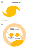 |
Fig. 1. Expected geometry of an MBBH in the presence of a circumprimary disk only (panel a) and in the presence of a circumbinary disk (panel b). In that case, the system is composed of three main features: a CBD, accretion streams, and mini-disks. |
Synergies between future observatories like Athena (Advanced Telescope for High ENergy Astrophysics; Nandra et al. 2013) and LISA are expected to provide constraints on the evolutionary paths leading to SMBHs and improve the detection of MBBHs. LISA will be able to detect mergers of massive black holes and with Athena it may be possible to detect MBBHs before merger. Indeed, as sub-parsec MBBHs in the LISA mass range approach merger, the X-ray modulation produced by the relativistic Doppler boosting of the mini-disks should be detectable. Following the coalescence of the massive black holes, the X-ray Integral Field Unit (X-IFU, Barret et al. 2023) on board Athena should provide important information on the MBBH environment, notably the density, temperature, and chemical enrichment, probing the history of MBBH evolution and formation. However, it may be possible to make some headway in understanding the evolution of SMBHs using current data and observatories. Many confirmed MBBHs and dual active galactic nuclei (AGN) at kiloparsec separation have already been discovered (e.g. Komossa et al. 2003; Bianchi et al. 2008; Fu et al. 2011; Husemann et al. 2018; Voggel et al. 2022; Koss et al. 2011; Trindade Falcão et al. 2024) but close sub-parsec MBBHs are yet to be confirmed. Possibly the best close MBBH candidate is OJ 287 (Sillanpaa et al. 1988). OJ 287 is a BL Lacertae object located at a redshift z = 0.306. It shows periodic outbursts in its optical and X-ray light curve approximately every 12 years (Sillanpaa et al. 1988), possibly due to interactions between the two black holes and their immediate environments. However, the MBBH nature causing the observed flares in OJ 287 has recently been contested, as the model predicted a flare in 2022 that has not yet been observed (e.g. Gorbachev et al. 2024). Other close sub-parsec MBBH candidates have been proposed, such as the galaxy Mrk 533, which shows a Z-shaped radio jet, interpreted by two orbiting massive black holes. Also, Runnoe et al. (2017) propose three quasars as possible sub-parsec MBBHs, identifying systematic and monotonic changes in their Hβ broad emission line profiles. Variability due to accretion flows in the optical light curves of close MBBHs is also expected (Artymowicz & Lubow 1996). It has been shown that AGN are more likely to appear in galaxy mergers, as the mergers trigger inward falling gas and thus accretion onto the galactic nuclei (e.g. Hopkins et al. 2008). Indeed, the fraction of AGN increases in galaxy mergers in comparison to non-mergers (e.g. Gao et al. 2020; Comerford et al. 2024; Lackner et al. 2014; Goulding et al. 2018). Furthermore, observational studies suggest that AGN activity peaks in the post-merging phase of galaxy mergers, as the star formation rate (SFR) and SMBH accretion rate increase in post-merger galaxies (e.g. Ellison et al. 2013; Satyapal et al. 2014). Therefore, detecting AGN activity may help to probe past galaxy mergers and could trace the presence of an MBBH.
In Section 2 of this paper we present our sample selection methodology and describe the different techniques we used to search for the periodicities in the light curves. We show the results of our investigation in Section 3. In Section 4, we compare our results with previous simulations, discuss the origin of the proposed periodicities, analyse X-ray spectra and fluxes of the suggested candidates and present the caveats of our work. Finally, we draw our conclusions in Section 5.
2. Methods
2.1. Sample selection and data processing
In 2015, Graham et al. (2015) undertook a systematic search for close SMBH binaries in quasars of the Catalina Real-Time Transient Survey (CRTS) and report a list of 111 possible candidates. However, quasars are subject to statistical variations called red noise. As discussed by Vaughan et al. (2016), quasars initially proposed as MBBH candidates due to their optical sinusoidal modulation can be better modelled by a red noise process. This is due to the fact that quasar light curves can display seemingly periodic variations due to red noise, and, as proposed by Vaughan et al. (2016), it is essential to observe at least five periods to infer the presence of periodic behaviour. We revisited the Graham et al. (2015) sample of candidates and studied sources from the Chen et al. (2020) catalogue.
2.1.1. Graham et al. sample
We took all the candidates from the Graham et al. (2015) sample (magnitudes between 15 and 20) and included more recent data from the Zwicky Transient Factory (ZTF) to extend the baseline and determine whether the sinusoidal oscillations are sustained over a sufficiently long time period. CRTS observations were made using the Catalina Sky Survey (CSS) Schmidt telescope between 2006 and 2016 in the northern sky, covering around 33 000 square degrees. Magnitudes were measured in the V-band with a limiting magnitude between 20 and 21 (Drake et al. 2009). ZTF is a 48-inch Schmidt telescope located at the Palomar Observatory. It has a 47-square degree field of view and covers ∼30 000 square degrees in the northern sky. ZTF observations started in March 2018 and are still ongoing. They are performed on two-night cadence. Magnitudes are measured in the g, r, and i bands with a limiting magnitude of ∼20.5 (Bellm et al. 2019).
2.1.2. Chen et al. sample
In 2020, Chen et al. (2020) published a catalogue of periodic variable sources using ZTF Data Release 2 (DR2; Bellm et al. 2019), including sources with magnitudes down to r∼20.6. This catalogue contains 781 602 confirmed variable sources and 1 381 527 objects that are possibly variable. Most of these objects are stars, and since we are interested in MBBH candidates, we cross-correlated this catalogue with a galaxy catalogue, Glade+ (Dálya et al. 2022). Glade+ includes ∼23 million objects, separated into 22.5 million galaxies and ∼750 000 quasars. Glade+ is complete to a luminosity distance of 44 Mpc (Dálya et al. 2022). To we obtain statistically reliable results, we investigated sources in Chen et al. (2020) with at least 400 ZTF measurements in a single band. To download ZTF data, we used the Infrared Science Archive (IRSA) website to query the best match between the Glade+ position of the selected objects (right ascension (RA) and declination (Dec)) and the ZTF data, reducing the odds of mismatching sources, in a 0.4 arc seconds radius (Masci et al. 2019). We used a maximum radius of 0.4 arc seconds in order to include all good matches. Fig. 2 shows the distribution of the distance between the matched ZTF and Glade+ sources in our sample. We can clearly see that the number of sources remains similar above 0.4 arc seconds, as the majority of matches are between 0 and 0.4 arc seconds.
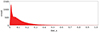 |
Fig. 2. Histogram representing the number of sources detected by ZTF in terms of the distance separation in arc seconds between the Glade+ and ZTF positions, for sources in Chen et al. (2020). |
In ZTF data, observations affected by clouds and/or the Moon are flagged with a catflag of 32 768. As suggested in the ZTF public data release, after downloading the ZTF data, we removed these bad observations by only keeping the data points with a catflag less than 32 768.
2.2. Sine model
As a first test, we fitted only the ZTF light curves for sources from Chen et al. (2020), to select those that appear to have sinusoidal modulation, using the sine function:
 (1)
(1)
where A, P, t0 and B are the amplitude, the period, the phase and the background of the model, respectively. Whilst it is clear that not all MBBHs will show strictly sinusoidal modulation, it is a first approach to search for modulation from such systems, as using more complex methods to search in such a large dataset is computationally prohibitive. We computed the reduced chi-squared value for each object and retained sources with a reduced chi-squared less than 1.3 which corresponds to a 4σ confidence interval that the sinusoidal modulation is a good description of the data. For these sources we added CRTS observations, when available, to evaluate whether or not the variability is sustained in both epochs. CRTS observations were retrieved from the Catalina Surveys Data Release 2 (CSDR) website1, using the sources RA and Dec to query the objects light curves. The sine model is a simplified model as it does not account for quasars’ intrinsic variability (see Sect. 2.5) and assumes accretion disks to be stable apart from the binary modulation. However, we used this model as a tool to identify possible MBBHs candidates, and more complex models are discussed below, considering that disk instabilities might be needed to fully explain the observed variability.
2.3. Data intercalibration
In order to compare the ZTF and CRTS observations of Graham et al. (2015) and Chen et al. (2020) sources, it was essential to perform an intercalibration, as they were taken with different instruments and different filters. We extended the CRTS light curves with ZTF data taken in the g filter. In order to take into account wavelength differences between the CRTS and ZTF-g filters, we intercalibrated CRTS and ZTF-g observations using the Python package PyCALI (Li et al. 2014), taking ZTF data as the reference, in the same way as Chen et al. (2024). Intercalibrating ZTF and CRTS data together takes into account colour variability and wavelength-dependent effects. This allowed us to compare both data sets to see whether or not they show the same variability. Moreover, in order to increase the signal-to-noise ratio, we grouped data points into bins spanning a maximum of 4 days. The new magnitude and errors in each bin were computed using Eqs. (2) and (3), respectively:
 (2)
(2)
 (3)
(3)
where μ, xi, σ(μ), σi and N correspond to the new calculated magnitude on the binned data point, the magnitude of each observed data point, the new calculated error on the binned data point, the magnitude error of each observed data point in the bin interval, and the number of observations in the considered bin, respectively. Also, to limit stochastic effects, we discarded sources with less than 25 CRTS observations after binning.
2.4. Fitting technique
To find the best fit sinusoid to the intercalibrated light curves, we used the nested sampling Monte Carlo algorithm MLFriends (Buchner 2016, 2023), using the Ultranest2 package (Buchner 2021) to derive the posterior probability distribution of the model parameters. Ultranest computes the posterior distribution probability by integrating the marginal likelihood, Z (Eq. 4) over the entire parameter space, where L(D|θ) is the likelihood function and π(θ)dθ is the prior probability density of the parameters, θ (Buchner 2019).
 (4)
(4)
The nested sampling technique consists of zooming towards best-fit models in the whole parameter space by regularly increasing the likelihood threshold. For further information on nested sampling, see Buchner (2019). Ultranest allows us to calculate the posterior distribution of the parameters and their standard deviations for the sinusoid, considering a set of priors; see Table 1. Considering the sampling of the data and the gaps in the light curve, we used a flat period prior between 500 and 2500 days to obtain a reliable number of cycles. We describe the other priors used for the fitting in Table 1. To ensure that the parameter space was correctly sampled, we used 400 live points during the fit. After calculating the posterior distribution for each light curve of the final sample, which contained variable CRTS and ZTF observations, we selected sources that showed a similar period for both data sets in the Graham et al. (2015) and Chen et al. (2020) samples.
Prior distribution for the sine function used to fit the data.
2.5. Damped random walk
AGN exhibit variability in all wavebands. Quasars, which are SMBHs actively accreting matter, display intrinsic optical variability called red noise. Distinguishing between red noise and variability caused by a binary system is a hard task and Vaughan et al. (2016) show that apparently sinusoidal variations might be caused by red noise. The damped random walk (DRW) model, a first-order continuous autoregressive model or CAR(1) process, is used to represent the optical stochastic variability in quasars (Kelly et al. 2009).
The DRW is defined by an auto-covariance function of the form
 (5)
(5)
where τ and c correspond to the characteristic timescale and total variance of the DRW, respectively (Vaughan et al. 2016). In order to introduce the DRW model, we used the Gaussian process (GP) Python package celerite (Foreman-Mackey et al. 2017). A GP model is composed of a mean function μθ(x) and a covariance or “kernel” function kα(xn,xm). The log-likelihood of a GP model L(θ,α) is by
 (6)
(6)
where rθ=y−μθ(t) is the vector of residuals and K is the covariance matrix with elements given by  where δnm is the Kronecker delta and k(tn,tm) the covariance function. We used the covariance function k(|tn−tm|) = aexp(−νbend×|tn−tm|), which is of a similar form to the DRW auto-covariance function and where a is the variance of the DRW. The power spectral density (PSD) of the DRW model has the form of a bending power law νγ, with ν the frequency and γ being 0 and smoothly bending to −2 above the bending frequency, νbend. In order to test our light curves with the DRW model, we fitted the DRW kernel to the light curves of our candidates using the nested sampling package Ultranest (see Section 2.4). Randomly sampling a and νbend from the best-fitting parameter distribution derived with the nested sampling fitting, we simulated 10 000 light curves for each source using the (Timmer & König 1995) algorithm. We sampled the simulated light curves at the same rate as the binary candidates and calculated their
  to evaluate their goodness of fit. We compared the calculated
  for the DRW and the sine model, which gives a probability of the preferred model for each object in our sample.
2.6. Generalised Lomb-Scargle periodogram
In order to further confirm our tentative periodicities, we computed the generalised Lomb-Scargle periodogram (GLS; Zechmeister & Kürster 2009) using the frequency range corresponding to the period prior described in Table 1, for each source retained from the Graham et al. (2015) and Chen et al. (2020) samples. The GLS is a period-finding technique for irregularly sampled light curves. The highest peaks in the GLS periodogram correspond, in general, to the most likely periods. To assess the significance of a given peak, we followed the methodology described by O’Neill et al. (2022) and computed the global p-value of the highest peak in each calculated GLS, i.e., the probability of detecting a peak of this power at any given frequency. This method consists of simulating 10 000 light curves following a DRW PSD (see Section 2.5). The bending frequency of the PSD is defined by νbend = 1/2πτ (see Eq. 5). Using τ calculated in the DRW, we ensured that the whole PSD was properly sampled. The simulated light curves were generated using the same method as described in Section 2.5 and were sampled at the same rate as the tested light curves. Firstly, for a given source, we computed the probability of the highest peak in its GLS periodogram by computing the probability that peak of this power can be reproduced in the simulated light curve at this specific frequency. This probability is called the single p-value. However, spurious periodicities due to red noise can occur at every frequency. So, to evaluate the global significance of a given candidate, we computed the single p-value of the highest peak in each of the 10 000 simulated light curves and determined the global significance, called the global p-value, of the candidate by calculating how many times the simulations produce a single p-value probability lower than the peak candidate.
2.7. A more realistic model
The pure sinusoidal model is a simple model that we used to find potential MBBH candidates. However, AGN are variable objects due to instabilities in the accretion disk. Thus, in the case of an MBBH, the sinusoidal variability should be modulated by red noise. We tested our candidates with a more realistic model composed of a DRW GP kernel (as described in Section 2.5) to account for the red noise modulation added to a sine function. We fitted the light curves for our proposed candidates with the DRW model using the nested sampling algorithm (see Section 2.4). The prior distributions used for the sine function are described in Table 1. To assess whether this model is preferred over the DRW model described in Sect. 2.5, we computed the Bayes ratio. The Bayes ratio, R, is defined as the ratio between the marginal likelihoods, or evidence, of the two models:
 (7)
(7)
In order to interpret the computed Bayes ratio, we adopted the widely used Jeffreys scale (Jeffreys 1939). Values of R in the range 3.2<R<10 and R>10 are, respectively, substantial or strong evidence for the presence of sinusoidal variability in a DRW model. R<1 indicates that the DRW model is preferred over the DRW plus sine modulation model.
2.8. Gravitational decay
The orbital decay due to gravitational wave emission is linked to the inspiral motion of the binary and it is determined analytically through post-Newtonian approximations. The gravitational wave emission of the inspiral motion is related to the separation of the binary. Indeed, the binary's time to merge tm, which depends on the energy loss through gravitational wave emission, is associated with the binary separation according to the power-law function,  (in geometric units G=c = 1, Peters 1964):
 (8)
(8)
where, M is the total mass of the binary and ν is the symmetric mass ratio parameter ν=M1M2/M2, with M1 and M2 the masses of the primary and secondary black holes in the binary, respectively. However, the orbital separation is also linked to the orbital period,  . Thus, for a given period, it is possible to compute, in units of M, the expected binary separation and the orbital decay due to gravitational wave emission, assuming a given mass ratio. However, for milliparsec separation MBBHs, the change of the period due to the emission of gravitational waves is thought to be longer than the time span of the observations used here. We discuss this further in Sect. 4.2.
3. Results
We investigated the Graham et al. (2015) sample of MBBH candidates. Out of 111 possible candidates, 89 sources also have ZTF observations. Fitting intercalibrated CRTS and ZTF data for all 89 objects, we find 26 objects that show similar variability in the CRTS and ZTF data.
We rejected 58 candidates, as the ZTF variability was clearly different from the CRTS variability (see, for example, Fig. 3, top panel). Lastly, for five sources there were insufficient ZTF data to draw reliable conclusions as there was less than half a period of ZTF observations. After cross-matching Chen et al. (2020) with Glade+ (Dálya et al. 2022), we identified 21 862 variable objects referenced either as galaxies or quasars. We fitted the ZTF data for those 21 862 objects with a sine function and selected sources with  , reducing this to 1010 galaxies. We extended their ZTF light curves with CRTS observations and fitted the intercalibrated data altogether. Out of the initial sample of 1010 galaxies, 10 showed consistent variability between CRTS and ZTF observations. We display in Appendix A the CRTS and ZTF light curves of all 36 objects, the CRTS and ZTF observations are, respectively, black and red dots. Note, however, that in the joint light curves, the
  remains quite high for some fits due to some scatter in the data. Graham et al. (2015) identify between 2 and 3 cycles per proposed candidate; for the 36 objects, we identify between ∼3 and 5 cycles for each candidate by extending the light curves using both CRTS and ZTF data. This is close to the number of periods that Vaughan et al. (2016) propose to infer periodic behaviour. We give the SDSS spectral redshift in Table B.1. This allows us to estimate the expected separation of the binary candidates, using redshift-corrected periods, supposing equal masses for the two black holes and using the mass estimates of Rakshit et al. (2020) (see Fig. 4). These mass estimates were obtained using continuum luminosity and Hβ, Mg(II) and C(IV) width measurements in SDSS optical spectra. The results are presented in Table B.1.
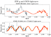 |
Fig. 3. Top: CRTS (black) and ZTF-g (red) intercalibrated light curve for a rejected candidate from the Graham et al. (2015) sample. Bottom: CRTS (black) and ZTF-g (red) intercalibrated light curve for an accepted candidate from the Graham et al. (2015) sample. |
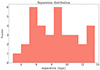 |
Fig. 4. Calculated separation distribution considering circular orbits and equal mass black holes in the binaries. |
The highest peaks in the GLS periodogram for the 36 sources give the same periods, within the error bars, as those inferred through fitting the data (see Table B.1). In Figure 5 we show an example of the GLS periodogram for the quasar SDSS J133654.44+171040.36.
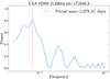 |
Fig. 5. GLS periodogram of the source SDSS J133654.44+171040.3. The period indicated from the strongest peak is in agreement with the fitted period from Ultranest. |
After modelling the light curves with the damped random walk, as described in Section 2.5, we compared the results to those obtained with the sinusoidal fit. The characteristic timescale, τ, found for our sources is similar to the value inferred for quasars as the mean τ in the sample of 36 candidates is ∼125 days (e.g. MacLeod et al. 2010; Burke et al. 2021). For the 36 sources, the sine model gives a better fit, as the  remains higher in the 104 simulated light curves. Using the more realistic model incorporating red noise into the sinusoidal modulation, as described in Section 2.7, the posterior period distributions resulting from the nested sampling computation peak at similar periods but with larger uncertainties than the sine-only model for most of our sources (see Table B.1). We show in Fig. 6 the posterior period distribution for a typical candidate. The Bayes ratio, R, calculated to compare this model with the pure DRW model gives a low value (R<1) for 30 sources, preferring the DRW-only model. Five sources have a Bayes ratio 1<R<3.2 indicating that the two models are equivalent. Finally, one object, J141425+171811, shows strong evidence for the DRW and sine model, as R is greater than seven. However, as discussed in Sect. 4, the Bayes ratio analysis might be inconclusive as it remains low even in the presence of sinusoidal modulation, because of the sparse, noisy data.
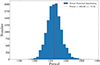 |
Fig. 6. Period posterior distribution for the source SDSS J133654.44+171040.3 using a red noise plus sine modulation model. |
The periods found for each object with the pure sine model, the Lomb-Scargle periodogram, and the sine-modulated red noise model are comparable and are in general consistent within the error bars (see Fig. 7). For the 36 sources, we computed the significance of the highest peaks in their GLS periodograms using the method described in Section 2.6. The significance of the peaks remains quite low for some of the objects, due to the quality of the data and the low number of cycles (three to five). These tests do not completely rule out the red noise origin and additional multi-wavelength evidence is needed to confirm the MBBH possibility.
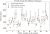 |
Fig. 7. Periods and uncertainties for the candidates in Table B.1 with the different techniques applied. The good agreement of the results from the different techniques can be clearly seen. |
We performed the initial periodicity analysis in the g-band. Additionally, we investigated the light curves with ZTF data in the r-band. We compared the light curves from the two wavebands in an additional check for periodicity. We find the same period in both the r- and the g-band light curves for each galaxy. We also compared the amplitudes of the two bands to constrain the origin of the emission. Figure 8 shows the intercalibrated light curves of SDSS J133654.44+171040.3 for ZTF data taken in the r-band (top) and g-band (bottom). The periodicities are compatible within 3σ, but the amplitude of the oscillation in the g-band is slightly greater; values are given in Table B.1. The increased variability in the blue is expected for MBBHs (Cocchiararo et al. 2024), but can also be observed in single black hole quasars (Vanden Berk et al. 2004).
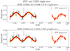 |
Fig. 8. Light curve of SDSS J133654.44+171040.3. Top: CRTS data (black) and ZTF data (red) taken in the r-band. Bottom: CRTS data (black) and ZTF data (red) taken in the g-band. |
4. Discussion
Validating MBBH candidates through light curve analysis is a challenging task. From our initial sample of 1099 sources from our selected ZTF data and the Graham et al. (2015) sample, we identify sinusoidal modulation in the CRTS and the ZTF data sets independently. Of these, 36 sources show similar periodicities in the CRTS and ZTF data. We show in Appendix A the lightcurves of the identified candidates. However, for other objects, when fitted together, the periodic variations identified in individual data sets are different. As an example of such unmatched periodicities, we show in the top panel of Fig. 3 the light curve of the quasar HS1630+2355. HS1630+2355 is a quasar from the Graham et al. (2015) sample to which we added ZTF data. We can see that CRTS data exhibit apparently periodic sinusoidal variations which do not match the ZTF data. According to Eq. (8), and if we consider the variability to probe the orbital period of the binary, the change of period due to the emission of the gravitational waves is too small for this separation scale to explain the observed variation in periodicity. Thus, we assigned this difference in identified periodicities to red noise and discarded the binary scenario to explain the variability. Out of the 89 sources for which there are ZTF observations, we discarded 58 of them as the identified variability observed in CRTS data is not seen in ZTF observations. In the final sample of MBBH candidates, all of our candidates have data spanning between three and five cycles, necessary to help rule out red noise behaviour. We determine similar periods through the Lomb-Scargle analysis and the DRW plus sine model, further reinforcing the likelihood of the presence of periodic modulation, which also lends support to the idea that these galaxies are home to close binary black holes. However, in most of our sources, the Bayes ratio indicates that the DRW model is preferred or is equivalent to the DRW plus a sinusoidal modulation. In order to estimate the Bayes ratio when a sine modulation is present, we simulated light curves with a sine modulation added to a DRW model for each candidate and computed the Bayes ratio. The parameters of the DRW and the sinusoidal modulation (i.e. a, νbend, A, B, P and t0) were set to the best values derived from the fitting of the DRW plus sine model to each candidate. The amplitude of the periodic modulation added in the simulated light curves is ∼0.1−0.2 magnitudes. The variance of the DRW process modelled in the simulations remains lower than the amplitude of the sinusoidal modulation by one order of magnitude for each candidate. The simulated light curves have the same sampling and error bars as the candidates. Despite the fact that we introduced a sinusoidal modulation, we retrieve simulated light curves with lower Bayes ratios than the candidate MBBH Bayes ratios (see, for example, Fig. 9, where R is lower than the lowest R calculated for our proposed candidates). R in the simulated light curves goes as low as ∼0.001. This is likely due to the paucity and low signal-to-noise ratio of the data. Therefore, completing the light curves with additional data taken with the ZTF or the upcoming Vera C. Rubin Observatory will be crucial to confirm which model is more probable.
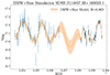 |
Fig. 9. Simulated light curve with a DRW and a sine modulation. The light curve has the same sampling and error bars as the candidate J083349.55+232809.0. The orange envelope corresponds to 1σ uncertainty of the best DRW plus sine fitted model. |
In addition, we checked the SDSS optical spectra of the candidates looking for broadening or asymmetries in the optical lines that could indicate the presence of a binary. However, no definitive evidence for binarity is visible because of the separation of the candidates and the limited spectral resolution.
4.1. Comparison with simulations
Some of the candidates in our sample are from the Chen et al. (2020) catalogue, which gives periodic sources found in ZTF DR2. As DR2 only covers a small part of the sky, see Fig. 10, this creates a selection bias. As a result, the candidates that we retrieved from this catalogue are grouped in the area with the most observations. We calculated the expected number of sub-parsec MBBH candidates at redshift z<1 in the Universe, extrapolating from our candidates. The MBBH candidates we propose have been found with joint CRTS and ZTF observations and the ZTF and CRTS surveys cover around 30 000 square degrees on the sky (Drake et al. 2009). Thus, extrapolating to the whole sky area and considering a homogeneous distribution, we could expect to find 19 sub-parsec supermassive binary quasars at a redshift z<1. Volonteri et al. (2009) found that they are relatively rare objects, with only around ten objects at z<0.7, but growing by a factor of ≈5−10 for a redshift z<1. Our result is slightly lower, as our study might not be complete due to the magnitude limitations of the surveys. Furthermore, our sample seems representative of the whole sample, as the total mass of the objects in our sample is quite high, with only two objects with a mass lower than 108 M⊙ and 20 objects with a mass higher than 109 M⊙ (see Fig. 11). This is expected, as the detection lifetime of MBBHs increases with the binary mass (Haiman et al. 2009). However, our number of candidates is higher than expected from Kelley et al. (2019), as they compute the CRTS survey to be able to detect between 0.2 and 5 binaries. Therefore, our list of candidates might contain a significant number of false positives.
 |
Fig. 10. Number of observations per CCD quadrant in ZTF DR2, in galactic coordinates centred at l,b = 0,0. Left: Number of observations made in r filter. Right: Number of observations made in the g filter. |
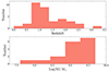 |
Fig. 11. Top: Histogram representing the redshift distribution of proposed MBBH candidates. Bottom: Histogram representing the Log(M) distribution of proposed MBBH candidates. |
4.2. Physical interpretation
We can see that the identified periods are the same in the r and g filters and that the fitted amplitudes differ slightly but are the same within the error for each candidate; see Table B.1. These fitted amplitudes are systematically higher in the g-band (the average amplitude in the blue filter is 0.167 and in the red filter it is 0.145), suggesting that the amplitude of the variability is higher in the g filter. Stronger modulation in the blue band is suggestive of an accretion disk origin (e.g. Cocchiararo et al. 2024). However, a similar increase in the variability in the blue can be seen in regular quasars (Vanden Berk et al. 2004). Different origins for the observed periodicity are plausible, such as a blob of gas orbiting in the CBD, referred to as the ‘lump’ (Farris et al. 2015a; Tang et al. 20183; Mignon-Risse et al. 2024; of plausible instability origin: Mignon-Risse et al. 2023); a periodic accretion flow due to the secondary black hole being closer to the inner edge of the circumbinary disk (Artymowicz & Lubow 1996); quasi-periodic oscillations due to the beat frequency between the orbital frequency and the frequency of the blob of gas in the CBD (e.g. Bowen et al. 2019; Mignon-Risse et al. 2024); or Doppler-boosting emission from the orbiting mini-disks (D’Orazio et al. 2015). Indeed, the relativistic effects due to the orbiting black holes would periodically boost or dim the emitted light of mini-disks moving towards or away from us.
In Fig. 12 we show the theoretical orbital separation under the geometric unit system G=c = 14. This unit system allows for direct comparison between different MBBH sources, since spatial scales are then normalised by the gravitational radius and can be used to estimate the region of gravitational influence of the MBBH. The separation is derived from the observed variability period, corrected for the redshift, and assuming Keplerian orbits and equal-mass binaries (though the mass ratio has a negligible influence on the period in these units), depending on the physical timescale on which the variability occurs: the orbital period P, the semi-orbital period P/2, or the lump (blob) period ∼4−10 P (e.g. Shi et al. 2012; Noble et al. 2012; Westernacher-Schneider et al. 2022; Mignon-Risse et al. 2023) which gives the error bars. This representation helps us to see if the orbital separation is consistent with the MBBH geometry associated with the assumed variability origin (see Fig. 1). Indeed, the larger the separation in the BBH, the less likely it is to possess a CBD, as it would require a larger angular momentum budget for the infalling gas building the CBD, in which case the variability might not be attributed to the lump. We can reasonably assume that BBHs with an orbital separation larger than 1000 M are unlikely to host a CBD. On the one hand, variability in the orbital or semi-orbital period can occur both in circumprimary disks (e.g. via accretion modulation produced by the m = 2 spiral arms) and CBD configurations (e.g. via Doppler boosting of the mini-disks, D’Orazio et al. 2015). The circumprimary disk scenario would be more likely for systems with an orbital separation of 100−1000 M. On the other hand, since the lump period is larger than the orbital period, the derived orbital separation is consistently smaller. As a consequence, except for two sources (J152157.02+181018.6 and J141425.92+171811.2), we get an orbital separation of ≲100 M which is compatible with a CBD configuration and therefore with the lump origin. Hence, interestingly, neither circumprimary disc nor CBD geometry can be ruled out here.
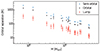 |
Fig. 12. Orbital separation as a function of M, depending on the origin of the modulation (semi-orbital, orbital, or due to the lump's orbit). The orbital separation is given in units of the total MBBH mass M, under the geometric unit system G=c = 1. For the lump-origin points, the error bars are obtained by considering a lump period between 4 P and 10 P. |
To briefly discuss the implications for the time to merger; if the variability is at the orbital or semi-orbital period, all systems are more than 105 days away from merger. In that case, the decrease in the period due to gravitational wave emission is indeed too small to be perceived, as can be expected. However, if the variability is at the lump period, the MBBH could be as close as 600 days before merger, and five of our candidates have a time to merger of less than 10 years: J160730.33+144904.3, J134855.92−032141, J081133.43+065558.1, J083349.55+232809.0 and J104941.01+085548.4. For these systems, the impact of the inspiral motion on the lump-related modulation period may not be negligible and depends also on the time at which MBBH-CBD decoupling occurs (Farris et al. 2015b). From a theoretical point of view, the survival of the lump-related modulation close to merger is still uncertain and calls for dedicated studies. It is, however, very unlikely that five sources have such a short time to merger, so it is highly likely that most, if not all, show modulation due to the binary orbit or semi-orbit. To confirm the origin, further data are necessary.
Other diagnostics can be used to rule out some of the aforementioned scenarios. If the detected emission is due to Doppler boosting of the mini-disks, the variability is expected to be stronger in the UV and the X-rays (De Rosa et al. 2019). Multi-wavelength observations would therefore be useful to help constrain the variability, yet difficult considering the timescales of the detected periodicities. Two sources in our sample, J123527.36+392824.0 and UM 234, have been observed once in X-ray with the XMM-Newton observatory. They show typical AGN spectra, well modelled with an absorbed power law and black body (see Fig. 13); parameters are shown in Table 3. If we suppose an expected geometry as described in Fig. 1, d’Ascoli et al. (2018) show that, for a black hole of 106 M⊙, the soft X-ray emission (∼1 keV) is dominated by the CBD and the mini-disks, while the hard X-ray part (>1 keV) is of coronal origin and found to originate entirely from the mini-disks. Considering the redshift and the masses of the two sources we expect their X-ray spectra to be mainly dominated by the coronal emission of the mini-disks. This is, indeed, what is seen. However, this kind of spectrum is also typical in single type I AGN.
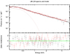 |
Fig. 13. Top: UM 234 X PN (black) and MOS2 (red) spectra modelled with an absorbed power law and black body. Bottom: Residuals of the applied model. |
Galaxy merger studies show that major galaxy mergers can trigger black hole activity, as the AGN evolves from a type II to a type I AGN closer to the end of the merger (e.g. Netzer 2015, and references therein). Then, detecting type I AGN emission could help trace a past galaxy merger (see Section 1). The sources in our sample from Chen et al. (2020) are galaxies, as they were selected by cross-matching with the galaxy catalogue Glade+. Even though only a fraction of our candidates were selected as they are AGN (notably those from the Graham sample), optical spectroscopy from SDSS and X-ray detections using the eRASS DR1 catalogue (Merloni et al. 2024) in the 0.2−2.3 keV band (see Table 2) indicates that all 36 candidates that we propose as MBBHs are actually quasars. This could provide further evidence for their binary black hole nature. We note that the eROSITA catalogue contains data for half the sky, and 18 out of 36 of our candidates fall within the footprint of this catalogue (see Fig. 14).
 |
Fig. 14. Aitoff projection of the eRASS1 DR1 main catalogue. Our candidates’ coordinates are represented with black dots. |
Candidate MBBHs eROSITA sources.
J123527.36+392824.0 and UM 234 X-ray model parameters.
In order to determine if these MBBH candidates accrete at fairly high rates, as expected if they are the result of mergers (e.g. Ellison et al. 2013; Satyapal et al. 2014), we tried to estimate the accretion rate as a percentage of the Eddington rate. Out of the 18 candidates in the eRASS DR1 footprint, 7 objects are detected with eROSITA. The median limiting flux for an extragalactic source in the eRASS1 DR1 main catalogue is 6 × 10⁻¹⁴ erg cm−2 s−1 (Merloni et al. 2024), so we consider this value as an upper limit for non-detected candidates in the catalogue. We show in Table 2 the 18 candidates in the part of the sky covered by the eRASS1 catalogue, along with their redshift, detected flux or upper limit, their predicted flux assuming that they radiate at 20% of their Eddington luminosity, and their computed luminosity. The predicted flux was calculated using the bolometric to X-ray correction proposed by Duras et al. (2020). The detected fluxes or upper limits are compatible with the very high accretion rate of 20% Eddington, except in the case of J115445+244646, which is the only source that shows a flux significantly lower than the predicted flux, putting an upper limit on its accretion rate around 5% of its Eddington accretion rate. These high accretion rates indicate a large reservoir of matter available to be accreted, which may originate from a previous merger (see, for example, Section 1).
We cannot determine if the X-ray flux varies over the orbital period as there is insufficient data in this catalogue version. Future versions will provide further data. If there is a modulation and it is due to periodic Doppler boosting, this would give constraints on the angle at which we are observing the system, as this effect cannot be seen if the object is observed face-on, while the variability amplitude is at a maximum when the orbit is seen edge-on.
4.3. Other possible candidates
For the sources with too little data, it is even more difficult to differentiate between modulations arising due to binarity or due to red noise. These candidates require many more observations to be considered good MBBH candidates, but we nonetheless created a catalogue of possible candidates, for which further observations are required. This catalogue of possible candidates contains 221 objects.
We show in Fig. 15 the Log(M) and redshift distribution of sources in this catalogue. We can see in Fig. 15 that the mass distribution of sources in our catalogue is concentrated towards high values with a mean log(M) value of 8.95. This result is expected for an MBBH population, as discussed in Sect. 4. In the redshift distribution, we can see two peaks; one around a redshift of 1 and the other around a redshift of 2.3. We can see that the number of candidates increases as the redshift increases between 0.5 and 1.0, as predicted by Volonteri et al. (2009). As we probe a larger volume, the chances of detecting more candidates rises. Also, as the number of candidates increases with redshift, it naturally shifts the mass distribution towards high values, as lower-mass black holes cannot be detected due to the limiting magnitudes of the surveys. The second peak is likely to emerge from the distribution of galaxies in the Glade+ catalogue (see Fig. 16), which is compiled from several different surveys and is therefore inhomogeneous in redshift and sky position.
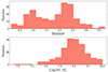 |
Fig. 15. Top: Histogram representing the redshift distribution of possible candidates. Bottom: Histogram representing the Log(M) distribution of possible candidates |
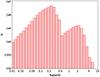 |
Fig. 16. Redshift distribution of galaxies in the Glade+ catalogue. |
4.4. Caveats
Whilst we have identified some sources that seem to have fairly reliable periods, we cannot be sure that these are indeed MBBHs. Indeed, the periods identified may not be due to a binary system but could be caused by other physical processes, or even instabilities occurring in single black hole disks. There is still a chance that the modulation may be due to red noise. Indeed, due to sparse data and low signal-to-noise ratio, the tests performed are unable to discriminate between a DRW model and a DRW plus sinusoidal modulation. Therefore, continued monitoring with current and future surveys, such as the Vera C. Rubin Telescope, will help to confirm these periods. Furthermore, our search focused on finding sinusoidal modulation in optical light curves, so we may miss periodic modulation that differs from a strictly sinusoidal curve, such as that which may be observed from eccentric orbits such as OJ 287 (Sillanpaa et al. 1988).
5. Conclusions
We identify 36 MBBH candidates through the detection of between three and five cycles of sinusoidal modulation in their optical light curves. These periods are corroborated through GLS analysis. The sparse and noisy data prevent us from establishing a clear statistical preference for the periodic model, regardless of the method used. The amplitude of the variability seems to be stronger in g-band than the r-band, as expected for MBBHs. Furthermore, the sources with X-ray observations show typical AGN-like spectra, which is also expected for MBBHs as mergers can trigger AGN activity. We emphasise that the sine model is a simplified model used to identify MBBH candidates but further investigation with more complex models to account for AGN variability might be needed to rigorously explain the observed variability. In the binary scenario, the observed periodicity can be explained by different physical origins, such as periodic accretion flow, Doppler-boosting modulation of the mini-disks, or a lump orbiting in the circumbinary disk. Multi-wavelength follow-up to look for UV or X-ray variability would be a good way to test the binarity of our candidates. Extrapolating from our sample, we determine the number of sub-parsec MBBH candidates at z<1, which is consistent with simulations. Also, we reject 58 objects previously proposed to be MBBHs (Graham et al. 2015) by using additional ZTF data and demonstrating that the sinusoidal modulation was not sustained over many periods. Finally, we created a catalogue of possible MBBH candidates that show some evidence for periodic modulation, but further observations are required to confirm this. The MBBHs at z<1 and with orbital periods between a week and a few years are expected to produce gravitational waves in the nanohertz band accessible to the PTA experiments. We are currently undertaking a targeted search for our z<1 candidates in the PTA data. Additionally, future surveys, such as the upcoming Rubin Observatory's Legacy Survey of Space and Time (LSST, Ivezić et al. 2019), will be useful to help confirm these candidates. Our method does not account for modulation that deviates from a sinusoidal behaviour such as what has been observed for OJ 287 (Sillanpaa et al. 1988) and our sample is likely to be only a fraction of the total population of MBBHs.
Data availability
Full Table C.1 is available at the CDS via anonymous ftp to cdsarc.cds.unistra.fr (130.79.128.5) or via https://cdsarc.cds.unistra.fr/viz-bin/cat/J/A+A/699/A55
Acknowledgments
The authors are grateful to the anonymous referee for careful reading of the paper and the excellent suggestions that helped improve this work. The authors acknowledge funding from the French National Research Agency (grant ANR-21-CE31-0026, project MBH_waves). NW and VF also acknowledge support from the CNES. Based on observations obtained with the Samuel Oschin Telescope 48-inch and the 60-inch Telescope at the Palomar Observatory as part of the Zwicky Transient Facility project. ZTF is supported by the National Science Foundation under Grants No. AST-1440341 and AST-2034437 and a collaboration including current partners Caltech, IPAC, the Weizmann Institute for Science, the Oskar Klein Center at Stockholm University, the University of Maryland, Deutsches Elektronen-Synchrotron and Humboldt University, the TANGO Consortium of Taiwan, the University of Wisconsin at Milwaukee, Trinity College Dublin, Lawrence Livermore National Laboratories, IN2P3, University of Warwick, Ruhr University Bochum, Northwestern University and former partners the University of Washington, Los Alamos National Laboratories, and Lawrence Berkeley National Laboratories. Operations are conducted by COO, IPAC, and UW Funding for SDSS-III has been provided by the Alfred P. Sloan Foundation, the Participating Institutions, the National Science Foundation, and the U.S. Department of Energy Office of Science. The SDSS-III website is http://www.sdss3.org/. SDSS-III is managed by the Astrophysical Research Consortium for the Participating Institutions of the SDSS-III Collaboration including the University of Arizona, the Brazilian Participation Group, Brookhaven National Laboratory, Carnegie Mellon University, University of Florida, the French Participation Group, the German Participation Group, Harvard University, the Instituto de Astrofisica de Canarias, the Michigan State/Notre Dame/JINA Participation Group, Johns Hopkins University, Lawrence Berkeley National Laboratory, Max Planck Institute for Astrophysics, Max Planck Institute for Extraterrestrial Physics, New Mexico State University, New York University, Ohio State University, Pennsylvania State University, University of Portsmouth, Princeton University, the Spanish Participation Group, University of Tokyo, University of Utah, Vanderbilt University, University of Virginia, University of Washington, and Yale University. RMR acknowledges funding from Centre National d’Etudes Spatiales (CNES) through a postdoctoral fellowship (2021–2023). RMR has received funding from the European Research Concil (ERC) under the European Union Horizon 2020 research and innovation programme (grant agreement number No. 101002352, PI: M. Linares).
In Tang et al. (2018), the assumed gas temperature is ∼10 times higher than in other theoretical studies (e.g. Roedig et al. 2014; d’Ascoli et al. 2018), resulting in X-ray rather than optical emission for the CBD.
In this unit system, spatial scales in physical units, denoted d′, are simply given by d′=d (M/1 M⊙)×1.477 km, where d is the spatial scale in geometric units.
References
- Agazie, G., Anumarlapudi, A., Archibald, A. M., et al. 2023, ApJ, 952, L37 [NASA ADS] [CrossRef] [Google Scholar]
- Amaro-Seoane, P., Aoudia, S., Babak, S., et al. 2013, GW Notes, 6, 4 [Google Scholar]
- Amaro-Seoane, P., Audley, H., Babak, S., et al. 2017, ArXiv e-prints [arXiv:1702.00786] [Google Scholar]
- Amaro-Seoane, P., Andrews, J., Arca Sedda, M., et al. 2023, Liv. Rev. Relat., 26, 2 [NASA ADS] [CrossRef] [Google Scholar]
- Armitage, P. J., & Natarajan, P. 2002, ApJ, 567, L9 [NASA ADS] [CrossRef] [Google Scholar]
- Artymowicz, P., & Lubow, S. H. 1996, ApJ, 467, L77 [NASA ADS] [CrossRef] [Google Scholar]
- Barret, D., Albouys, V., Herder, J. -W. D., et al. 2023, Exp. Astron., 55, 373 [NASA ADS] [CrossRef] [Google Scholar]
- Bate, M. R., & Bonnell, I. A. 1997, MNRAS, 285, 33 [NASA ADS] [CrossRef] [Google Scholar]
- Begelman, M. C., Blandford, R. D., & Rees, M. J. 1980, Nature, 287, 307 [Google Scholar]
- Bellm, E. C., Kulkarni, S. R., Graham, M. J., et al. 2019, PASP, 131, 018002 [Google Scholar]
- Bianchi, S., Chiaberge, M., Piconcelli, E., Guainazzi, M., & Matt, G. 2008, MNRAS, 386, 105 [CrossRef] [Google Scholar]
- Bowen, D. B., Mewes, V., Noble, S. C., et al. 2019, ApJ, 879, 76 [Google Scholar]
- Buchner, J. 2016, Stat. Comput., 26, 383 [Google Scholar]
- Buchner, J. 2019, PASP, 131, 108005 [Google Scholar]
- Buchner, J. 2021, J. Open Source Softw., 6, 3001 [CrossRef] [Google Scholar]
- Buchner, J. 2023, Stat. Surv., 17, 169 [NASA ADS] [CrossRef] [Google Scholar]
- Burke, C. J., Shen, Y., Blaes, O., et al. 2021, Science, 373, 789 [NASA ADS] [CrossRef] [Google Scholar]
- Chen, X., Wang, S., Deng, L., et al. 2020, ApJS, 249, 18 [NASA ADS] [CrossRef] [Google Scholar]
- Chen, Y. -J., Zhai, S., Liu, J. -R., et al. 2024, MNRAS, 527, 12154 [Google Scholar]
- Cocchiararo, F., Franchini, A., Lupi, A., & Sesana, A. 2024, A&A, 691, A250 [NASA ADS] [CrossRef] [EDP Sciences] [Google Scholar]
- Colpi, M. 2014, Space Sci. Rev., 183, 189 [Google Scholar]
- Combi, L., Lopez Armengol, F. G., Campanelli, M., et al. 2022, ApJ, 928, 187 [NASA ADS] [CrossRef] [Google Scholar]
- Comerford, J. M., Nevin, R., Negus, J., et al. 2024, ApJ, 963, 53 [NASA ADS] [CrossRef] [Google Scholar]
- Dálya, G., Díaz, R., Bouchet, F. R., et al. 2022, MNRAS, 514, 1403 [CrossRef] [Google Scholar]
- d’Ascoli, S., Noble, S. C., Bowen, D. B., et al. 2018, ApJ, 865, 140 [CrossRef] [Google Scholar]
- De Rosa, A., Vignali, C., Bogdanović, T., et al. 2019, New Astron. Rev., 86, 101525 [Google Scholar]
- Desvignes, G., Caballero, R. N., Lentati, L., et al. 2016, MNRAS, 458, 3341 [Google Scholar]
- D’Orazio, D. J., Haiman, Z., & Schiminovich, D. 2015, Nature, 525, 351 [Google Scholar]
- Drake, A. J., Djorgovski, S. G., Mahabal, A., et al. 2009, ApJ, 696, 870 [Google Scholar]
- Duras, F., Bongiorno, A., Ricci, F., et al. 2020, A&A, 636, A73 [NASA ADS] [CrossRef] [EDP Sciences] [Google Scholar]
- Ellison, S. L., Mendel, J. T., Patton, D. R., & Scudder, J. M. 2013, MNRAS, 435, 3627 [CrossRef] [Google Scholar]
- EPTA Collaboration & InPTA Collaboration (Antoniadis, J., et al.) 2024, A&A, 685, A94 [NASA ADS] [CrossRef] [EDP Sciences] [Google Scholar]
- Farris, B. D., Duffell, P., MacFadyen, A. I., & Haiman, Z. 2015a, MNRAS, 446, L36 [NASA ADS] [CrossRef] [Google Scholar]
- Farris, B. D., Duffell, P., MacFadyen, A. I., & Haiman, Z. 2015b, MNRAS, 447, L80 [NASA ADS] [CrossRef] [Google Scholar]
- Foreman-Mackey, D., Agol, E., Ambikasaran, S., & Angus, R. 2017, ApJ, 154, 220 [CrossRef] [Google Scholar]
- Foster, R. S., & Backer, D. C. 1990, ApJ, 361, 300 [NASA ADS] [CrossRef] [Google Scholar]
- Fu, H., Zhang, Z. -Y., Assef, R. J., et al. 2011, ApJ, 740, L44 [Google Scholar]
- Gao, F., Wang, L., Pearson, W. J., et al. 2020, A&A, 637, A94 [NASA ADS] [CrossRef] [EDP Sciences] [Google Scholar]
- Gorbachev, M. A., Butuzova, M. S., Nazarov, S. V., & Zhovtan, A. V. 2024, Astropart. Phys., 160, 102965 [Google Scholar]
- Goulding, A. D., Greene, J. E., Bezanson, R., et al. 2018, PASJ, 70, S37 [NASA ADS] [CrossRef] [Google Scholar]
- Graham, M. J., Djorgovski, S. G., Stern, D., et al. 2015, MNRAS, 453, 1562 [Google Scholar]
- Haiman, Z., Kocsis, B., & Menou, K. 2009, ApJ, 700, 1952 [CrossRef] [Google Scholar]
- Hopkins, P. F., Hernquist, L., Cox, T. J., & Kereš, D. 2008, ApJS, 175, 356 [Google Scholar]
- Husemann, B., Worseck, G., Arrigoni Battaia, F., & Shanks, T. 2018, A&A, 610, L7 [NASA ADS] [CrossRef] [EDP Sciences] [Google Scholar]
- Ivezić, Ž., Kahn, S. M., Tyson, J. A., et al. 2019, ApJ, 873, 111 [Google Scholar]
- Jeffreys, H. 1939, Theory of Probability (Oxford: Oxford University Press) [Google Scholar]
- Kelley, L. Z., Haiman, Z., Sesana, A., & Hernquist, L. 2019, MNRAS, 485, 1579 [NASA ADS] [CrossRef] [Google Scholar]
- Kelly, B. C., Bechtold, J., & Siemiginowska, A. 2009, ApJ, 698, 895 [Google Scholar]
- Komossa, S., Burwitz, V., Hasinger, G., et al. 2003, ApJ, 582, L15 [NASA ADS] [CrossRef] [Google Scholar]
- Koss, M., Mushotzky, R., Treister, E., et al. 2011, ApJ, 735, L42 [Google Scholar]
- Lackner, C. N., Silverman, J. D., Salvato, M., et al. 2014, ApJ, 148, 137 [Google Scholar]
- Li, Y. -R., Wang, J. -M., Hu, C., Du, P., & Bai, J. -M. 2014, ApJ, 786, L6 [Google Scholar]
- MacLeod, C., Ivezic, Z., Kozlowski, S., et al. 2010, Am. Astron. Soc. Meet. Abstr., 215, 433.26 [Google Scholar]
- Masci, F. J., Laher, R. R., Rusholme, B., et al. 2019, PASP, 131, 018003 [Google Scholar]
- Merloni, A., Lamer, G., Liu, T., et al. 2024, A&A, 682, A34 [NASA ADS] [CrossRef] [EDP Sciences] [Google Scholar]
- Mignon-Risse, R., Varniere, P., & Casse, F. 2023, MNRAS, 520, 1285 [NASA ADS] [CrossRef] [Google Scholar]
- Mignon-Risse, R., Varniere, P., & Casse, F. 2024, MNRAS, submitted [Google Scholar]
- Nandra, K., Barret, D., Barcons, X., et al. 2013, ArXiv e-prints [arXiv:1306.2307] [Google Scholar]
- Netzer, H. 2015, ARA&A, 53, 365 [Google Scholar]
- Noble, S. C., Mundim, B. C., Nakano, H., et al. 2012, ApJ, 755, 51 [NASA ADS] [CrossRef] [Google Scholar]
- O’Neill, S., Kiehlmann, S., Readhead, A. C. S., et al. 2022, ApJ, 926, L35 [CrossRef] [Google Scholar]
- Papaloizou, J., & Pringle, J. E. 1977, MNRAS, 181, 441 [NASA ADS] [CrossRef] [Google Scholar]
- Peters, P. C. 1964, Phys. Rev., 136, 1224 [Google Scholar]
- Rakshit, S., Stalin, C. S., & Kotilainen, J. 2020, ApJS, 249, 17 [Google Scholar]
- Reardon, D. J., Zic, A., Shannon, R. M., et al. 2023, ApJ, 951, L6 [NASA ADS] [CrossRef] [Google Scholar]
- Roedig, C., Krolik, J. H., & Miller, M. C. 2014, ApJ, 785, 115 [NASA ADS] [CrossRef] [Google Scholar]
- Runnoe, J. C., Eracleous, M., Pennell, A., et al. 2017, MNRAS, 468, 1683 [Google Scholar]
- Satyapal, S., Ellison, S. L., McAlpine, W., et al. 2014, MNRAS, 441, 1297 [Google Scholar]
- Savonije, G. J., Papaloizou, J. C. B., & Lin, D. N. C. 1994, MNRAS, 268, 13 [NASA ADS] [CrossRef] [Google Scholar]
- Shi, J. -M., & Krolik, J. H. 2015, ApJ, 807, 131 [NASA ADS] [CrossRef] [Google Scholar]
- Shi, J. -M., Krolik, J. H., Lubow, S. H., & Hawley, J. F. 2012, ApJ, 749, 118 [Google Scholar]
- Sillanpaa, A., Haarala, S., Valtonen, M. J., Sundelius, B., & Byrd, G. G. 1988, ApJ, 325, 628 [NASA ADS] [CrossRef] [Google Scholar]
- Tang, Y., Haiman, Z., & MacFadyen, A. 2018, MNRAS, 476, 2249 [NASA ADS] [CrossRef] [Google Scholar]
- Timmer, J., & König, M. 1995, A&A, 300, 707 [Google Scholar]
- Trindade Falcão, A., Turner, T. J., Kraemer, S. B., et al. 2024, ApJ, 972, 185 [Google Scholar]
- Vanden Berk, D. E., Wilhite, B. C., Kron, R. G., et al. 2004, ApJ, 601, 692 [Google Scholar]
- VanderPlas, J. T. 2018, ApJS, 236, 16 [Google Scholar]
- Vaughan, S., Uttley, P., Markowitz, A. G., et al. 2016, MNRAS, 461, 3145 [Google Scholar]
- Verbiest, J. P. W., Lentati, L., Hobbs, G., et al. 2016, MNRAS, 458, 1267 [Google Scholar]
- Voggel, K. T., Seth, A. C., Baumgardt, H., et al. 2022, A&A, 658, A152 [NASA ADS] [CrossRef] [EDP Sciences] [Google Scholar]
- Volonteri, M., Madau, P., & Haardt, F. 2003, ApJ, 593, 661 [Google Scholar]
- Volonteri, M., Miller, J. M., & Dotti, M. 2009, ApJ, 703, L86 [NASA ADS] [CrossRef] [Google Scholar]
- Westernacher-Schneider, J. R., Zrake, J., MacFadyen, A., & Haiman, Z. 2022, Phys. Rev. D, 106, 103010 [NASA ADS] [CrossRef] [Google Scholar]
- Xu, H., Chen, S., Guo, Y., et al. 2023, RAA, 23, 075024 [NASA ADS] [Google Scholar]
- Yu, Q. 2002, MNRAS, 331, 935 [Google Scholar]
- Zechmeister, M., & Kürster, M. 2009, A&A, 496, 577 [CrossRef] [EDP Sciences] [Google Scholar]
Appendix A: 36 Candidates CRTS/ZTF intercalibrated lightcurves
We show below the CRTS (black) and ZTF (red) lightcurves of the 36 potential MBBH candidates we found. Dashed green line represents the best fitted sine function. Orange envelope is the 3σ best fitted sine function.
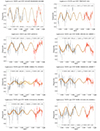 |
Fig. A.1. CRTS (black) and ZTF-g (red) intercalibrated light curves of proposed MBBH candidates. |
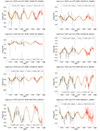 |
Fig. A.2. CRTS (black) and ZTF-g (red) intercalibrated light curves of proposed MBBH candidates. |
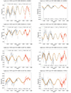 |
Fig. A.3. CRTS (black) and ZTF-g (red) intercalibrated light curves of proposed MBBH candidates. |
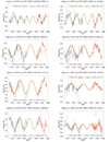 |
Fig. A.4. CRTS (black) and ZTF-g (red) intercalibrated light curves of proposed MBBH candidates. |
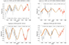 |
Fig. A.5. CRTS (black) and ZTF-g (red) intercalibrated light curves of proposed MBBH candidates. |
Appendix B: Results Table
36 MBBH Candidates results
Appendix C: 20 First rows of the additional candidates catalogue
Additional candidates catalogue
All Tables
All Figures
|
Fig. 1. Expected geometry of an MBBH in the presence of a circumprimary disk only (panel a) and in the presence of a circumbinary disk (panel b). In that case, the system is composed of three main features: a CBD, accretion streams, and mini-disks. |
| In the text | |
|
Fig. 2. Histogram representing the number of sources detected by ZTF in terms of the distance separation in arc seconds between the Glade+ and ZTF positions, for sources in Chen et al. (2020). |
| In the text | |
|
Fig. 3. Top: CRTS (black) and ZTF-g (red) intercalibrated light curve for a rejected candidate from the Graham et al. (2015) sample. Bottom: CRTS (black) and ZTF-g (red) intercalibrated light curve for an accepted candidate from the Graham et al. (2015) sample. |
| In the text | |
|
Fig. 4. Calculated separation distribution considering circular orbits and equal mass black holes in the binaries. |
| In the text | |
|
Fig. 5. GLS periodogram of the source SDSS J133654.44+171040.3. The period indicated from the strongest peak is in agreement with the fitted period from Ultranest. |
| In the text | |
|
Fig. 6. Period posterior distribution for the source SDSS J133654.44+171040.3 using a red noise plus sine modulation model. |
| In the text | |
|
Fig. 7. Periods and uncertainties for the candidates in Table B.1 with the different techniques applied. The good agreement of the results from the different techniques can be clearly seen. |
| In the text | |
|
Fig. 8. Light curve of SDSS J133654.44+171040.3. Top: CRTS data (black) and ZTF data (red) taken in the r-band. Bottom: CRTS data (black) and ZTF data (red) taken in the g-band. |
| In the text | |
|
Fig. 9. Simulated light curve with a DRW and a sine modulation. The light curve has the same sampling and error bars as the candidate J083349.55+232809.0. The orange envelope corresponds to 1σ uncertainty of the best DRW plus sine fitted model. |
| In the text | |
|
Fig. 10. Number of observations per CCD quadrant in ZTF DR2, in galactic coordinates centred at l,b = 0,0. Left: Number of observations made in r filter. Right: Number of observations made in the g filter. |
| In the text | |
|
Fig. 11. Top: Histogram representing the redshift distribution of proposed MBBH candidates. Bottom: Histogram representing the Log(M) distribution of proposed MBBH candidates. |
| In the text | |
|
Fig. 12. Orbital separation as a function of M, depending on the origin of the modulation (semi-orbital, orbital, or due to the lump's orbit). The orbital separation is given in units of the total MBBH mass M, under the geometric unit system G=c = 1. For the lump-origin points, the error bars are obtained by considering a lump period between 4 P and 10 P. |
| In the text | |
|
Fig. 13. Top: UM 234 X PN (black) and MOS2 (red) spectra modelled with an absorbed power law and black body. Bottom: Residuals of the applied model. |
| In the text | |
|
Fig. 14. Aitoff projection of the eRASS1 DR1 main catalogue. Our candidates’ coordinates are represented with black dots. |
| In the text | |
|
Fig. 15. Top: Histogram representing the redshift distribution of possible candidates. Bottom: Histogram representing the Log(M) distribution of possible candidates |
| In the text | |
|
Fig. 16. Redshift distribution of galaxies in the Glade+ catalogue. |
| In the text | |
|
Fig. A.1. CRTS (black) and ZTF-g (red) intercalibrated light curves of proposed MBBH candidates. |
| In the text | |
|
Fig. A.2. CRTS (black) and ZTF-g (red) intercalibrated light curves of proposed MBBH candidates. |
| In the text | |
|
Fig. A.3. CRTS (black) and ZTF-g (red) intercalibrated light curves of proposed MBBH candidates. |
| In the text | |
|
Fig. A.4. CRTS (black) and ZTF-g (red) intercalibrated light curves of proposed MBBH candidates. |
| In the text | |
|
Fig. A.5. CRTS (black) and ZTF-g (red) intercalibrated light curves of proposed MBBH candidates. |
| In the text | |
Current usage metrics show cumulative count of Article Views (full-text article views including HTML views, PDF and ePub downloads, according to the available data) and Abstracts Views on Vision4Press platform.
Data correspond to usage on the plateform after 2015. The current usage metrics is available 48-96 hours after online publication and is updated daily on week days.
Initial download of the metrics may take a while.