


| Issue |
A&A
Volume 711, July 2026
|
|
|---|---|---|
| Article Number | A239 | |
| Number of page(s) | 24 | |
| Section | Interstellar and circumstellar matter | |
| DOI | https://doi.org/10.1051/0004-6361/202557551 | |
| Published online | 20 July 2026 | |
ALMA-IMF
XXI. N2H+ kinematics in the G012.80 protocluster: Evidence of filament rotation and evolution
1
Departamento de Astronomía, Universidad de Conceptión,
Casilla 160-C,
4030000
Conceptión,
Chile
2
Instituto de Radioastronomía y Astrofísica, Universidad Nacional Autónoma de México,
Morelia,
Michoacán
58089,
Mexico
3
Franco-Chilean Laboratory for Astronomy, IRL 3386, CNRS and Universidad de Chile,
Santiago,
Chile
4
Scottish Universities Physics Alliance (SUPA), School of Physics and Astronomy, University of St. Andrews,
North Haugh,
St. Andrews
KY16 9SS,
UK
5
Univ. Grenoble Alpes, CNRS, IPAG,
38000
Grenoble,
France
6
INAF-Osservatorio Astrofisico di Arcetri,
Largo F. Fermi 5,
50125
Firenze,
Italy
7
Laboratoire d'Astrophysique de Bordeaux, Univ. Bordeaux, CNRS,
B18N, allée Geoffroy Saint-Hilaire,
33615
Pessac,
France
8
Department of Astronomy, University of Florida,
PO Box 112055,
Florida,
USA
9
Departamento de Astronomía, Universidad de Chile,
Las Condes,
7591245
Santiago,
Chile
10
Department of Astronomy, School of Science, The University of Tokyo,
7-3-1 Hongo, Bunkyo,
Tokyo
113-0033,
Japan
11
Instituto de Astrofísica de Andalucía (CSIC),
Glorieta de la Astronomía s/n,
18008
Granada,
Spain
12
Departament de Física Quàntica i Astrofísica (FQA), Universitat de Barcelona,
Martí i Franquès 1,
08028
Barcelona,
Catalonia,
Spain
13
Institut de Ciències del Cosmos (ICCUB), Universitat de Barcelona,
Martí i Franquès 1,
08028
Barcelona,
Catalonia,
Spain
14
Institut d'Fstudis Fspacials de Catalunya (IFFC), Fsteve Terradas 1, edifici RDIT,
Parc Mediterrani de la Tecnologia (PMT) Campus del Baix Llobregat – UPC
08860
Castelldefels (Barcelona),
Catalonia,
Spain
15
Departments of Astronomy and Chemistry, University of Virginia,
Charlottesville,
VA
22904,
USA
16
Instituto Argentino de Radioastronomía (CCT-La Plata, CONICFT; UNLP; CICPBA),
C.C. No. 5,
1894,
Villa Flisa,
Buenos Aires,
Argentina
17
Laboratoire de Physique de l'École Normale Supérieure, FNS, Université PSL, CNRS, Sorbonne Université, Université de Paris,
Paris,
France
★ Corresponding author: This email address is being protected from spambots. You need JavaScript enabled to view it.
Received:
3
October
2025
Accepted:
22
May
2026
Abstract
We characterize kinematic processes in the G012.80 protocluster. We primarily focused on the N2H+(1−0) emission to trace the dense and cold gas. Additionally, we used complementary lines such as DCN(3-2), H41α, C18O(2−1), and SiO(5−4), as well as continuum maps. We performed a N2H+ hyperfine spectral line fitting to analyze multiple velocity components and extract spectral parameters. We estimated velocity gradients, column densities, and line-mass profiles for the two main filaments in G012, which we named R1 and R2. The line-mass profiles follow λ(ω) = 5660M⊙pc−1 (ω/pc)0.30 for R1 and λ(ω) = 6943 M⊙pc−1(ω/pc)0.20 for R2. This is much larger than profiles of typical low-mass filaments. R1 and R2 show disparate position-velocity (PV) features. R1 exhibits a transverse velocity gradient of 10.4 km s−1 pc−1 and a few dense cores. This velocity gradient is interpreted with a simple rotation toy model when combined with the line-mass profile, and it corresponds to a rotational timescale of ~0.1 Myr. In contrast, R2 exhibits compact velocity structures (ΔV < 2 km s−1), likely due to collapse, as evidenced by the comparatively large number of massive cores and protostellar outflows. R2 is forming prestellar and protostellar cores at a rate of ~ 55.3 M⊙ Myr−1, with an efficiency similar to the Orion integral shaped filament (ISF). The R1 filament, in contrast, lacks protostellar cores and only contains a few prestellar cores, resulting in an estimated star formation rate of ~4.2M⊙ Myr−1, which is lower by more than an order of magnitude than that of R2. Combining gas kinematics, core incidence, and the line-mass profiles, we suggest that R1 is younger and still rotates, while R2 has evolved to collapse with a higher star formation rate. G012 thus hosts filaments at different evolutionary stages.
Key words: evolution / HII regions / ISM: kinematics and dynamics
© The Authors 2026
 Open Access article, published by EDP Sciences, under the terms of the Creative Commons Attribution License (https://creativecommons.org/licenses/by/4.0), which permits unrestricted use, distribution, and reproduction in any medium, provided the original work is properly cited.
This article is published in open access under the Subscribe to Open model. This email address is being protected from spambots. You need JavaScript enabled to view it. to support open access publication.
1 Introduction
Protoclusters, or embedded star clusters, are gas-dominated regions in which stars are actively forming. Unlike clusters, where gravity is dominated by the stars themselves, protoclusters are defined by the gravitational effect of the dense gas from which the stars emerge (Stutz 2018). It is crucial to study these regions for understanding the early stages of star cluster formation, particularly the formation of high-mass stars, which significantly affect their surroundings through outflows, radiation, and supernovae, and which predominantly form in clusters (Motte et al. 2018). These massive stars play a vital role in shaping galaxy evolution and estimating star formation rates, highlighting the importance of studying protoclusters and their internal assembly processes to understand key astrophysical phenomena.
Molecular gas is often organized in filaments: elongated and dense gas structures that are the birth sites of prestellar and protostellar cores. These cores are embedded within the filaments and represent the sites of star formation. They provide a natural link for investigating the kinematic relation between dense gas and forming protostars. Filaments can be detected at the scale of molecular clouds, but also at small protocluster scales (<1 pc); they constitute the immediate gas reservoir from which cores accrete (e.g., Kirk et al. 2013; Stutz & Gould 2016; Zhou et al. 2022; Hacar et al. 2023; Louvet et al. 2024). In cluster-forming environments, filaments are not expected to be static structures. High-mass star formation (HMSF) environments are characterized by deep gravitational potentials, high gas surface densities, stellar feedback, and strong gas motions (e.g., inflow, turbulence, and outflow), all of which can significantly modify the kinematic state of the filamentary gas. Observational signatures encoded in molecular spectra such as longitudinal and transverse velocity gradients (e.g., Álvarez-Gutiérrez et al. 2021, 2024; Sandoval-Garrido et al. 2025), velocity-coherent substructures (e.g., González Lobos & Stutz 2019; Cunningham et al. 2023), or multiple velocity components (e.g., Csengeri et al. 2011a,b) can trace gas-accretion flows inside filaments (e.g., Kong et al. 2019; Liu et al. 2023), gravitational collapse, rotational motions, or the effect of ionizing feedback and gas ejection (e.g., Galván-Madrid et al. 2010, 2024; Towner et al. 2024; Armante et al. 2024). It is particularly important to distinguish between these scenarios in massive protoclusters, where different theoretical frameworks predict different roles for filamentary gas. For example, models of global hierarchical collapse suggest that filaments funnel material toward cluster centers through gravitation-driven inflows (e.g., Vázquez-Semadeni et al. 2019), while alternative scenarios emphasize converging turbulent flows (e.g., Padoan & Nordlund 2002) or rotationally supported structures as mechanisms shaping the filament dynamics (e.g., André et al. 2014). Therefore, the study of the kinematics of dense gas in filaments at protocluster scales provides a direct way to test how mass is assembled and redistributed during the formation of stellar clusters.
To study these processes in a massive cluster-forming environment, we focused on the G012.80 protocluster (hereafter G012), which is one of the 15 nearby massive protoclusters observed by the Atacama Large Millimeter/submillimeter Array (ALMA) Initial Mass Function (IMF) Large Program1 (ALMAIMF LP, Motte et al. 2022). Specifically, G012 is an active and massive (M870 μm = 1.7 × 10³ M⊙, see Motte et al. 2022) star-forming region centered on the W33 main clump, with a trigonometric parallax distance of 2.4 kpc (Immer et al. 2013) and a local standard of rest velocity of VLSR = 37 km s−1 estimated from maser velocities (Immer et al. 2014). A central star cluster with spectral types from O7.5 to B1.5 has been reported (Immer et al. 2013), along with evidence of dissociation of complex molecules on small scales (e.g., Immer et al. 2014). Detections of HC3N, CO outflows, class I methanol masers, H``II``` regions, OB star clusters, and a high abundance of cores indicate that G012 is an optimal testbed for studying HMSF in an evolved protocluster, particularly the mechanisms regulating the distribution and kinematics of dense gas in a feedback-rich environment (e.g., Haschick & Ho 1983; Yu et al. 2019; Xie et al. 2023; Armante et al. 2024). To probe the dense gas kinematics in G012, we focused on diazenylium (N2H+; e.g., Bergin & Langer 1997; Caselli et al. 1995; Bergin & Tafalla 2007; Lippok et al. 2013; Tatematsu et al. 2008; Busquet et al. 2011; Gómez et al. 2022). This nitrogen-bearing molecule is characterized by lower depletion levels onto dust grains and was first detected in the interstellar medium by Thaddeus & Turner (1975). For the N2H+(1−0) transition, the critical density ranges from 2.0 × 104 cm−3 at 100 K to 6.1 × 104 cm−3 at 10 K (Shirley 2015), indicating the conditions under which this line becomes an effective tracer. Variations in the observed N2H+ emission can therefore be linked to changes in the physical conditions of the protocluster (Tobin et al. 2013; Tafalla et al. 2021; Yu et al. 2022).
When the kinematics and dense gas emission traced by molecules like N2H+ are scrutinized in individual protoclusters, multiple evolutionary stages (or generations of stars) emerge within a single region (Cunningham et al. 2023; Pouteau et al. 2023; Armante et al. 2024). This motivates detailed studies of evolved protoclusters with internal structures at potentially different evolutionary stages. The search for correlations between the kinematic properties of these dense gas structures (e.g., Stutz & Gould 2016; Álvarez-Gutiérrez et al. 2021; Xu et al. 2023; Álvarez-Gutiérrez et al. 2024; Reyes-Reyes et al. 2024; Sandoval-Garrido et al. 2025) and their line-mass profiles (e.g., Stutz 2018) sets the stage for developing observationally driven physical models of protocluster evolution as stellar mass is assembled. In this context, we focused on the two dominant internal cold dense gas structures in G012 identified with N2H+ (1−0). These structures have the form of coherent filaments that show evidence of either rotation or collapse. We characterize the dense gas kinematics and key physical parameters in the protocluster, with particular emphasis on these two main filaments.
This paper is organized as follows. In Sect. 2 we detail the ALMA-IMF dataset and core catalogs for the G012 protocluster. In Sect. 3 we analyze the N2H+ moment maps, PV diagrams, column density, and N2H+ core velocities in the region. We perform a detailed analysis of the two dominant cold dense gas filamentary structures in Sect. 4, focusing on average velocity gradients and line-mass profiles. In Sect. 5, we apply a rotation toy model to the observed dense gas kinematics in the R1 filament. In Sect. 6, we discuss potential evolutionary scenarios by comparing the kinematics and other observables (e.g., core incidence). Finally, we summarize our main conclusions in Sect. 7.
Spectral line setup.
2 Data
We used observations from the ALMA telescope provided by the ALMA-IMF LP. The line parameters for N2H+ and additional tracers are summarized in Table 1.
2.1 ALMA-IMF datacubes
We employed N2H+(J=1−0) observations at a frequency of 93.1734 GHz. We followed a similar data reduction procedure as Álvarez-Gutiérrez et al. (2024) and Sandoval-Garrido et al. (2025). N2H+ observations were cleaned using the ALMA-IMF imaging pipeline2 (Cunningham et al. 2023) and the version 5.6.0 of The Common Astronomy Software Applications package (CASA, CASA Team 2022). We used the imcontsub task to subtract the continuum emission from the N2H+ line emission. To estimate the continuum emission, we only considered emission-free channels in the range of 12−20 km s−1, where we applied a linear fit using fitorder = 0. To recover the cloud emission at all available scales, we combined observations of the 7m and 12m arrays with total power data (TP). To do this, we used the task feather. This combination also allowed us to recover the missing flux, visible as negative bowls in the inter-ferometric spectral data produced by the lack of zero-spacing. We obtained a fully integrated multi-scale emission dataset. The resulting N2H+ datacube contained a total of 217 velocity channels over a range from 12 km s−1 to 61 km s−1, with a spectral resolution of 0.23 km s−1 and a final beam size of ~2.3" (see Table 1), corresponding to ~5.5 kau at the source distance. In Fig. 1 we display Spitzer observations at 8 μm (red), 4.5 μm (green) and 3.6 μm (blue) along with an N2H+ integrated-intensity contours at 25 and 100 K km s−1 (left panel) and N2H+ integrated-intensity map at a signal-to-noise ratio (S/N) > 12 (right panel; see Appendix A for the S/N selection criteria). The N2H+ integrated-intensity map reveals a filamentary and clumpy morphology that traces the dense gas in the region, with a clear absence of emission toward the protocluster center, consistent with the potential chemical destruction of N2H+ in the vicinity of the young stellar cluster (see Sect. 6.1).
In addition to the N2H+ data, we used complementary spectral lines previously analyzed in ALMA-IMF studies. These include the H41α recombination line (Galván-Madrid et al. 2024), which traces HII regions associated with ionizing sources in the protocluster center; DCN(J=2−1; Cunningham et al. 2023), which traces more compact and warmer emission than N2H+; SiO (J=5−4; Towner et al. 2024), used to analyze potential outflow features; and C18O (J=2−1; Koley et al. 2025), which traces compact emission in the central region of the protocluster and more extended and fainter emission in the surroundings.
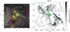 |
Fig. 1 Multiwavelength view and molecular gas distribution of the G012 protocluster. Left panel: Spitzer RGB composite figure of the G012 protocluster at 8 μm (red), 4.5 μm (green), and 3.6 μm (blue). The two cyan contours trace the N2H+ integrated-intensity emission at 25 and 100 K km s−1, respectively. Right panel: N2H+ integrated-intensity map with contours at 25 and 100 K kms−1, corresponding to an S/N > 12, shown in black (same levels as in the left panel). The blue boxes highlight the two main filamentary structures, R1 and R2, with estimated lengths of 0.56 pc for both. We show the average spectra of the two regions in the insets. The black curve represents the data within the black boxes. The red markers represent ionizing regions (crosses), radio sources (plusses), and infrared sources (dots) detected in the region by Haschick & Ho (1983). The green contours show continuum emission from the Atacama Large Millimeter/submillimeter Array Band 6 observations (Ginsburg et al. 2022b). The black ellipse in the bottom right corner represents the beam size of the N2H+ data. |
2.2 ALMA-IMF dense core catalogs
Louvet et al. (2024) constructed the first core catalog of the full ALMA-IMF sample based on the 1.3 mm and 3 mm continuum emission. They used the toolkit Getsf (Men'shchikov 2021) to identify compact continuum sources. In G012, they detected 57 dense cores with estimated masses of 0.6–6.2 M⊙ and temperatures of 25–100K. As a follow-up, Cunningham et al. (2023) used the DCN molecular line emission to study the core population from Louvet et al. (2024). For G012, they were able to estimate spectral parameters of 38 cores, including their line-of-sight velocities. Deeper, Armante et al. (2024) constructed a catalog of G012 cores complementing dust continuum emission (at 1.3 mm and 3 mm) with molecular emission from the 12CO(2−1), SiO(5−4), CH3OCHO, and CH3CN spectral lines. They classified the cores as prestellar or protostellar, finding a total of 94 detections. Additionally, Motte et al. (2025) provided new mass, temperature, and luminosity estimates for cores in the remaining ALMA-IMF protoclusters using radiative transfer modeling. For G012, they found protostellar and prestellar cores distributed over mass ranges of 0.3–9.5 M⊙.
To complement these data and provide a more complete characterization of G012, we used all these core catalogs in our analyses. In particular, we estimate in the Appendix F new velocities for 48 cores from these previous catalogs.
Global parameters of the R1 and R2 filaments.
3 Analysis of the N2H+ data cube
By modeling the hyperfine structure of the N2H+ (as described in Appendix A), we derived key kinematic parameters and simultaneously identified multiple velocity components in the N2H+ spectra. We adopted a similar fitting procedure as Sandoval-Garrido et al. (2025) to model the N2H+ emission. We used the hyperfine line structure model provided by version V.1.0.1 of the PySpecKit spectroscopic analysis toolkit (Ginsburg et al. 2022a). The vast majority of spectra that we inspected are well characterized by either one or two velocity components (see Appendix A). Hence, we applied a fitting model with up to two components, using parameters such as excitation temperature (Tex), optical depth (τ), velocity centroid (Vc), and velocity dispersion (σ). The model-fitting results showed that G012 is characterized by two main velocity structures separated by ~2.5 km s−1, which we defined as the first velocity component (FVC) and the second velocity component (SVC). We adopted 35.6 km s−1 as the reference velocity (see Appendix A) to separate them: FVC refers to spectra with velocities below this value, and SVC refers to those above it. Using the FVC and SVC structures, we further explored the kinematics of G012. First, we reviewed moment maps, which provide a detailed look at the velocity centroid and dispersion patterns in the region and of the particular filamentary structures R1 and R2 (see Fig. 1). We then constructed PV diagrams of the entire region to capture the velocity gradients and dynamical behavior of the protocluster. We also estimated column densities and masses in G012 in order to set constraints on the gas mass and density profiles in the region.
3.1 Moment maps
In Fig. 2, we display the N2H+ integrated-intensity (moment zero map, upper panels), velocity center (moment one map, middle panels), and velocity dispersion (moment two map, bottom panels) maps of the FVC and SVC. In the N2H+ integrated-intensity map, G012 is characterized by a filamentary distribution in the plane of the sky (POS). Specifically, we highlight the two prominent filaments with blue boxes (see also Fig. 1), which are the focus of this study, hereafter called R1 and R2. These structures were identified based on the visual inspection of prominent and kinematically well-separated filamentary structures, where the kinematic patterns described below are more clearly distinguished. However, to complement this more visual inspection, we also applied a more automated method, as described in Appendix B.
The R1 filament is largely dominated by the FVC (see Fig. 2, left panel), which displays one pronounced velocity gradient across the filament. The R1 mean centroid velocity and line width are 〈V〉 = 34.4 km s−1 and 〈σ〉 = 0.81 km s−1, respectively. In contrast, the R2 filament is dominated by the SVC (see Fig. 2, right panel), which exhibits more homogeneous velocity structures. The mean centroid velocity and line width for R2 are 〈V〉 = 36.8 km s−1 and 〈σ〉 = 0.75 km s−1, respectively (see Table 2 for global parameters of the main filaments). Additionally, at the center of G012, we observe an absence of N2H+ emission that may be related to the destruction of the molecule in the region (see Sect. 6). To analyze this absence, we reviewed the integrated-intensity maps of the fitted complementary tracers in Fig. A.3. The C18O emission (upper left panel) traces more extended gas than N2H+ and is primarily distributed around the H41α bubbles (bottom left panel). In addition, we identified high C18O integrated-intensity structures in the surroundings of the R1 and R2 filaments. The SiO integrated intensity reveals elongated features in the R2 filament (upper right panel). Specifically, one perpendicular outflow feature is observed at the top of R2, related to a previously detected hot core (Armante et al. 2024). Furthermore, DCN, which is associated with increased star formation, traces some of the densest parts of the filamentary structures in R1 and R2 (bottom right panel).
3.2 N2H+ PV diagrams
We used the technique developed in González Lobos & Stutz (2019) to construct the N2H+ intensity-weighted position velocity diagrams (e.g., Álvarez-Gutiérrez et al. 2021, 2024; Sandoval-Garrido et al. 2025). To obtain better-defined structures in PV space, we spatially rotated the N2H+ data cubes (45° with respect to the protocluster center) by vertically aligning the most predominant filaments. In Fig. 3, we show PV diagrams of the first velocity component (blue shades) and the second velocity component (green shades) structures. The upper left panel shows the integrated-intensity map after spatial alignment. In the upper right and bottom left panels, we display the PV diagrams perpendicular and parallel to the region, respectively. Additionally, we include the positions of previous cores detected in G012 (Cunningham et al. 2023; Louvet et al. 2024; Armante et al. 2024; Motte et al. 2025). For the PV diagrams, we show a representative timescale of 0.2 Myr3 based on the PV structures that are more strongly spread in velocity (ΔV > 3 km s−1). In addition to the main features mentioned above, we also highlight an elongated structure with high integrated intensity in the bottom left diagram, located at a velocity range (ΔV) of approximately −2 to 0 km s−1. This structure is spatially related to the R1 filament (see Sect. 4). The key features in the PV diagrams are listed below.
R2 reveals a set of characteristic twisting features (Fig. 3, bottom right panel) that are confined to a narrow velocity range (< 2 km s−1), in contrast to the broader velocity spread observed in R1.
The PV features are more spread out in velocity (ΔV > 3 km s−1 ; see the upper right panel in Fig. 3) in regions near H41α and SiO emission (see Fig. A.3), indicating short associated timescales. This potentially highlights the effect of stellar feedback close to the center of G012.
The R1 and R2 filaments reveal the most predominant and intricate PV structures.
The R1 filament exhibits a double-helix feature (Fig. 3, bottom right panel), spanning approximately ~3 km s−1 in velocity. This type of feature has been associated with filament rotation in other regions (e.g., Álvarez-Gutiérrez et al. 2021). We address this point in Sect. 5.
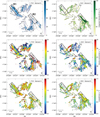 |
Fig. 2 N2H+(1−0) integrated intensity (upper panels), velocity centroid (middle panels), and velocity dispersion (bottom panels) of the FVC (left panels) and SVC (right panels). The black contours trace the N2H+ integrated-intensity emission at 25 and 100 K km s−1. The black boxes in all panels display the spatial location of the R1 and R2 filaments. The black ellipse in the bottom right corner represents the beam size of the N2H+ data. |
3.3 N2H+ column density
The column density and mass in protoclusters provide insights into the amount of material available for star formation. In order to estimate the N2H+ column density, we used the Tex, τ, and σ PySpecKit output parameters (see Appendix A). We applied the column density approximation outlined in Caselli et al. (2002a) and Redaelli et al. (2019), which is described as
 (1)
(1)
Here, ν represents frequency of the N2H+(1−0) emission, g = 3 is the statistical weight (degeneracy) of the upper energy level of the transition level, c is the light speed, A = 3.6e−5 s−1 is the Einstein coefficient, Eu = 4.47 K corresponds to the upper energy level of the transition, Q is the rotational partition function of N2H+, kB is the Boltzmann constant, and h is the Planckconstant (Shirley 2015; Redaelli et al. 2019).
To mitigate potential biases introduced by poorly defined fitting parameters (see Appendix A) and to prevent anomalies in the column density and relative abundance estimates, we excluded all pixels affected by systematic biases in τ and Tex. Specifically, we removed pixels where Tex = 150 K (the fitting upper limit) and τ < 0.2, which resulted in discarding 30% of the affected pixels (see Appendix D). We consider the final column density map as the sum of the FVC and the SVC column densities. Overall, the R1 column density distribution appear more interconnected, compact, and filamentary. In contrast, the R2 column density values are distributed more homogeneously, taking high values of about 1 × 1014 cm−2 in most of the region. We converted the N2H+ column density into mass, obtaining a respective N2H+ mass of 1.72 × 10⁻⁵ M⊙ in the entire protocluster. The two main filaments, R1 and R2, contribute approximately 12% and 17% of the N2H+ protocluster mass, respectively. Moreover, when considering the extended emission associated with these filaments (see Appendix B), their total contribution accounts for about 60 % of the total N2H+ mass, further emphasizing their importance in the kinematics and mass distribution of the region.
 |
Fig. 3 Position-position and position-velocity diagrams of the N2H+ observations. Upper left panel: G012 integrated intensity of FVC (blue shades) and SVC (green shades). We display the DCN cores from Cunningham et al. (2023) catalog with black pluses. The Armante et al. (2024) core catalog is divided into four categories: cores only detected with N2H+ (red crosses), cores only detected with DCN data (red circles), cores detected with N2H+ and DCN (red triangles), and cores detected neither in N2H+ nor DCN (black triangles). The symbol sizes are proportional to the estimated core mass. The black ellipse in the bottom right corner represents the beam size of N2H+ data. Upper right panel: PV diagram along the y-axis; the velocity axis is subtracted from the N2H+ systemic VLSR of the protocluster (35.5 km s−1). The black arrow illustrates a slope of 5 pc (km s−1 )−1, which corresponds to a timescale of ~0.2 Myr, that is, the timescales that approximately correspond to some of the extended structures in this PV diagram. At the top of R1, lies a wrapped (or double-helix) type velocity field with spreads of more than ~3 km s−1. On the other hand, R2 appears very compact in velocity along its extent, with small-scale spatial wiggles. Bottom left panel: PV diagram in the perpendicular direction compared to the upper right panel. This shows the emergence, albeit somewhat hidden in the overall velocity field, of an approximately uniform and extended gradient in R1 that is apparent near ΔX ~ 0.60 to 0.75 pc, ΔV ~ −2 to 0 km s−1. In contrast, R2 appears as the compact blob of cores (triangles and x-symbols) on the right-hand-side of the panel, characterized by the absence of an obvious gradient in position and velocity. Bottom right panel: zoomed PV diagrams of the main filaments R1 (left panel) and R2 (right panel), enclosed in the black boxes of the upper left panel. R1 presents a wrapping double-helix signature that is most obvious toward the top of the diagram and which is dominated by the FVC velocities. R2 exhibits comparatively compact velocity variations (ΔVmax~1.5 km s−1) along the filament and contains a high number of massive cores (1–3 M⊙). |
 |
Fig. 4 Left panel: relative abundance map in G012. The black contour highlights the mask of |

3.4 Relative abundance
In G012, previous estimates of the H2 column density map (Dell'Ova et al. 2024) did not provide the full spatial coverage achieved by the N2H+ map. Nevertheless, despite these limitations, particularly the incomplete coverage of the main filaments in the region, the map from Dell'Ova et al. (2024) remains the most suitable tool currently available for estimating the relative abundance in the region. We used the N2H+ column density to estimate the total mass (Mtot) in the protocluster as a whole and in areas where the H2 map lacks complete spatial coverage. First, we calculated the relative abundance in the N2H+ and H2 column density maps (see Fq. (2)) where we had coverage in both. To estimate this ratio, we reprojected the N2H+ image to match the pixel scale of the H2 data, which is slightly larger (with a pixel scale of 0.83"). Subsequently, we calculated the relative abundance map by taking the pixel-to-pixel ratio of the two maps,
 (2)
(2)
Here, N(N2H+) is the N2H+ column density map described above, and N(H2) is the H2 column density map from Dell'Ova et al. (2024). For the N(H2) map, we considered an S/N > 3 based on the ratio of the column density and the associated errors. In Fig. 4 (left panel) we present the resulting relative abundance map. We identify a clear trend in which the relative abundances values decrease toward regions associated with ionization (see Fig. 8 left panel, for a comparison between the N2H+ emission and the H41α distribution). This behavior likely reflects the effect of stellar feedback on the molecular gas distribution. We discuss this point further in Sect. 6.
We determined representative N2H+ relative abundance values using the mode of its distribution, a choice motivated by its stability under different binning and masking conditions (see Appendix D). We obtained a relative abundance of X(N2H+) = (0.93 ± 0.10) × 10−10 (see Figure 4, right panel), consistent with previous determinations (Caselli et al. 2002c; Sandoval-Garrido et al. 2025). This representative value was then applied to derive total H2 mass. Since these estimates will underpin the line-mass profiles presented in Sect. 4.2, we first validated our choice of mass map by calculating the line-mass profile in a section of the R2 filament covered by the N2H+ and Dell'Ova et al. (2024) column density maps (see Appendix F). We found variations of less than 28% between the two methods, indicating that the use of N2H+ to re-estimate the total H2 mass, and consequently, the line-mass profiles discussed in Sect. 4.2, is robust.
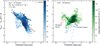 |
Fig. 5 Average velocity gradients perpendicular to R1 (left panel) and R2 (right panel) filaments. In both diagrams, the ΔV and Δr axes have the same range, allowing for a direct comparison of the slopes between the panels. In R1 the red line represents the linear fit weighted by the integrated-intensity points of the velocity gradient (VG). The associated VG timescale (τ) estimate is displayed in the upper left corner. In contrast, R2 lacks a clear velocity gradient structure as in R1 and is instead comparatively compact in its velocity distribution. In addition, we identified two different velocity distributions that spatially correspond to different regions in the R2 filament: 1) the most compact and central structure (compact feature) is related to the densest region of the filament; and 2) the most elongated feature is spatially related to the eastern edge of the R2 filament, characterized by elongated SiO emission. In the diagram, the lower intensity and scattered points represent regions surrounding the filament. |
4 R1 and R2 characterization
The R1 and R2 filaments are the predominant N2H+ integrated-intensity structures in the G012 protocluster. These regions present different velocity structures in PV diagrams (see Sect. 3), suggesting the presence of two different star-forming environments taking place in the same protocluster. In this section, we focus on the characterization of these two filaments with the aim to set constraints on their star-forming stage.
4.1 Average filament velocity gradients
As shown in Fig. 3 (bottom right panel), the R1 filament is associated with a potential signature of rotation, while R2 presents a relatively compact velocity distribution. We analyzed the velocity gradients perpendicular to the two filaments through average-velocity gradients estimations. We adapted the method described by Álvarez-Gutiérrez et al. (2021) for the filament rotation analysis and divided the procedure into the following steps:
We determined the total integrated intensity in each region (i.e., the moment 0 of the FVC and SVC, see Sect. 3) and calculated peak integrated-intensity values along the long axis of the two filaments in order to determine a representative filament ridge line (see Appendix C).
For each slice along the y-axis, we straightened the two filaments by centering the peak integrated intensity from the ridge line to a fixed arbitrary position. Then, each point of the integrated intensity, velocity centroid, and velocity dispersion maps had a projected radius to the center of the filament.
We generated ridge line-averaged PV diagrams as follows. For each point, at each radius from the ridge line, we plot the radial velocities as shown in Fig. 5. Here, the color of each point indicates their integrated intensity. These velocity versus radius diagrams therefore capture PV structures integrated over the length of the filament. If a given filament has a prominent velocity gradient approximately perpendicular to the ridge line, these diagrams will reveal these structures. Since the projected radius is measured perpendicular to the filament ridge line, a coherent velocity gradient in these velocity versus projected radius diagrams is naturally interpreted as rotation around the filament axis. This is the case for R1, while for R2, no such equivalently prominent structure is observed.
We applied a linear fit to the velocity gradient in the R1 filament using the integrated intensity as a statistical weight.
In Fig. 5, we show the R1 (left panel) and R2 (right panel) ridge line-averaged PV diagram described above. In this representation, a linear and elongated structure reflects a systematic change in velocity with projected radius, as expected from rotation around the filament axis. The global R1 velocity gradient (VG) has a magnitude of VG ~ 10.4 km s−1 pc−1 (with an associated statistical fitting error of ± 0.29 km s−1 pc−1). In R2, in sharp contrast to R1, we do not observe an equivalent global average velocity gradient. In contrast, R2 is dominated by a compact velocity structure, clumping at velocities around ~1 km s−1 in the center of the diagram. This compact feature traces the central and densest part of the filament. We also observe a more spread-out structure in projected radius and velocity extending up and to the left in the diagram and ending near - 0.05 pc, 0.75 km s−1 (elongated feature). This structure is approximately associated with the eastern edge of the R2 filament and has associated elongated SiO emission that likely traces protostellar outflows and shocks (Towner et al. 2024).
4.2 Line-mass profiles and associated 3D model quantities
The characterization of the mass distribution, and hence, of the gravitational potential, is a requirement for interpreting the kinematics in these systems since the gravitational field of the gas serves as governor of the dynamics of a system (e.g., Stutz 2018; González Lobos & Stutz 2019; Álvarez-Gutiérrez et al. 2021; Reyes-Reyes et al. 2024). We followed the formalism outlined in Stutz & Gould (2016) to estimate these line-mass profiles in the main filaments of the G012 protocluster. We first aligned the filament mass maps with respect to their ridge lines (see Appendix C). We used a box region to capture the densest parts of the two filaments (see Fig. 1) and constructed N2H+ cumulative mass distributions for both regions. As expected for elongated and dense structures, the cumulative mass distribution profiles in R1 and R2 are nearly linear (see Fig. F.1), indicating that the mass distribution along the filament is approximately uniform. This allowed us to derive an averaged line-mass profile as a function of projected radius from the ridge line over the entire filament. While the two distributions share this linear behavior, they differ in normalization: R2 is systematically shifted toward higher masses than R1. Following the formalism in Stutz & Gould (2016), we found that the line-mass profiles are well-described by power laws of the form
 (3)
(3)
where ω is the projected radius in the POS (or impact paramenter from the ridge line), γ corresponds to the index in the enclosed mass over length (M/L) versus projected radius diagram (see Fig. 6), and ζ is the M/L normalization constant. For R1 and R2, we obtained
 (4)
(4)
In Fig. 6, we display the M/L profiles of the R1 and R2 filaments (red and blue lines, respectively), along with other star-forming regions (dashed black lines) described below and in Table 3.
We followed Stutz & Gould (2016); Stutz (2018), and Álvarez-Gutiérrez et al. (2021) in estimating the density, gravitational potential, and acceleration assuming cylindrical 3D geometry. All quantities were estimated in the POS since we lack access to inclination information. We refer to these as "apparent" profiles following Álvarez-Gutiérrez et al. (2021). We estimated the apparent volume density as
 (5)
(5)
where for the R1 and R2 filaments, we obtained βR1 = 211.3 M⊙ pc−3 and βR2 = 181.3 M⊙ pc−3. We estimated the gravitational potential as
 (6)
(6)
where, considering the R1 and R2 parameters described above, we estimated ψR1 = 123.1 km2 s−2 and ψR2 = 269.3 km2 s−2.
Finally, we estimated the gravitational acceleration as follows:
 (7)
(7)
For R1 and R2, we obtained ξR1 =37.4 km2 s−2 pc−1 and ξR2 = 51.3 km2 s−2 pc−1, respectively.
Relative to other star-forming regions (see Fig. 6), the filaments in G012 exhibit significantly higher line-mass profiles that are up to three times more dense than extended regions such as the G351.77 protocluster (Reyes-Reyes et al. 2024). This trend remains even in more extended regions along the filaments, as detailed in Appendix B. The corresponding line-mass profile parameters, including the filament extensions, are listed in Table 3.
Line-mass profiles, volume density, gravitational potential, and acceleration distributions.
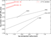 |
Fig. 6 Line-mass profile of the R1 and R2 filaments (red lines). The red shaded area represents the uncertainty in the two estimates, derived from the relative abundance uncertainty. This percentage therefore provides a lower limit to the error of 11% in both distributions. We include profiles of the Orion ISF (Stutz & Gould 2016), the ONC (Stutz 2018), the California L1482 region (Álvarez-Gutiérrez et al. 2021), and the G351.77 protocluster (Reyes-Reyes et al. 2024) with black lines. The main filaments of G012 reveal denser line-mass distributions than those found in other star-forming regions. |
4.3 Star formation rate and efficiency
The star formation rate (SFR) and efficiency (SFE) are critical parameters for understanding the current star formation activity, offering insight into the efficiency with which gas is converted into stars. To estimate the SFR (Eq. (8)), we assumed lifetimes based on observational studies of pre- and protostellar cores. Specifically, the lifetimes of prestellar cores vary significantly with environment and initial conditions, ranging from 0.5 to 2 Myr in low-mass regions (e.g., Jessop & Ward-Thompson 2000; Merín et al. 2008; Evans et al. 2009; Könyves et al. 2015) to as short as 0.05–0.24 Myr in high-mass cores, where collapse is driven by fast-converging flows (Csengeri et al. 2011a,b; Motte et al. 2018; Valeille-Manet et al. 2025). As cores evolve into protostellar phases, accretion becomes dominant, and the lifetimes decrease with increasing mass from ~0.5Myr for low-mass protostars (Megeath et al. 2022) to 0.1–0.3 Myr for high-mass cores (Duarte-Cabral et al. 2013; Valeille-Manet et al. 2025). Gravitational contraction, temperature increase, and accretion rates are strongly affected by the initial core mass and local conditions (Bontemps et al. 2010; Dunham et al. 2014).
For the SFR and SFE estimates, we used the formalism outlined in Megeath et al. (2022) and considered the G012 core masses provided in Motte et al. (2025). In R1 and R2, Armante et al. (2024) and Motte et al. (2025) identified a total of 16 cores. Fourteen of these are located in R2, and only two are in R1. These cores are classified as either prestellar or protostellar, with masses ranging from 0.3 to 3 M⊙. For our analysis, we adopted a prestellar timescale of 1.2 Myr, which is the expected value for prestellar cores in the mass range of 0.003–10 M⊙ (Könyves et al. 2015). We also used a protostellar lifetime of 0.5 Myr, assuming a low-mass protostellar regime around 0.5 M⊙ (Megeath et al. 2022). The two cores in R1 are classified as prestellar, while the R2 filament exhibits five cores in this phase. In addition, the R2 filament contains nine protostellar cores. Considering the pre- and protostellar lifetimes described above, we estimated the SFR as follows:
 (8)
(8)
Here, Mcores is the mass of the core population (prestellar and/or protostellar) and tcores is the approximate lifetime of the cores in million years. For R1 and R2, we obtained
SFRR1–prestellar = (4.24 ± 0.29) M⊙Myr−1,
SFRR2–prestellar = (12.1 ± 1.90) M⊙Myr−1,
SFRR2–protostellar = (43.2 ± 6.67) M⊙Myr−1,
SFRR2–total = SFRprestellar + SFRprotostellar = (55.3 ± 6.93) M⊙Myr−1.
Errors were estimated solely from the mass uncertainties reported in the Motte et al. (2025) catalog, without possible uncertainties on the adopted timescales. For instance, a lifetime of 0.3 Myr for the intermediate- to high-mass protostellar regime would increase the SFR to (71.9 ± 11.2) M⊙ Myr−1.
In addition, we estimated the SFE as
 (9)
(9)
In this case, Mcores represents the same core mass as we used for the SFR estimate, and Mcloud corresponds to the R1 or R2 filament mass (see Table 2). In R1 and R2, we obtained
SFER1–prestellar = (1.6 ± 0.1) × 10−3,
SFER2–prestellar = (3.3 ± 0.4) × 10−3,
SFER2–prestellar = (4.8 ± 0.4) × 10−3,
SFER2–total = SFEprestellar + SFEprotostellar = (8.1 ± 0.5) × 10−3.
In this case, we adopted the same assumptions for the core mass uncertainties as for the SFR. For the cloud (filament) mass, we assumed an 11% error, corresponding to the uncertainty associated with the relative abundance values in the region. Our estimates of SFR and SFE should be regarded as lower limits, since they are based exclusively on the population of pre- and protostellar cores traced by some specific tracers. Unlike nearby star-forming regions, more distant regions such as G012 require a more complete core census for accurate determinations. Overall, the SFR and SFE in R1 are lower by roughly an order of magnitude than in R2. This trend even persists in more extended filamentary regions (see Appendix B).
5 A filament rotation toy model applied to R1
In the N2H+ PV diagram, the R1 filament shows a helical pattern. This feature is also observed in the California L1482-S cloud and was attributed to filamentary rotation (Álvarez-Gutiérrez et al. 2021; Hsieh et al. 2021). In Fig. 3 (bottom right panel) we highlight this feature at the top of R1, which is also associated with a clear average-velocity gradient of ~ 10.4 km s−1 pc−1 (see Fig. 5, left panel).
To determine whether rotation or gravity is the dominant factor in the R1 filament, we compared the velocity gradient to the gravitational acceleration implied by the filament mass distribution. We applied the formalism from Álvarez-Gutiérrez et al. (2021) to estimate the centrifugal force associated with rotation of the R1 filament. We then calculated the ratio of the centrifugal and gravitational forces as follows:
 (10)
(10)
Here, Fc and Fg represent the centrifugal and gravitational forces, respectively. VG is the average-velocity gradient associated with the R1 filament rotation, ξ is the constant associated with the gravitational acceleration distribution (see Table 3), and θ represents the (unknown) inclination angle of the filament relative to the POS.
In Fig. 7, we show the resulting profile for the ratio of forces in the R1 filament (red line) compared to the L1482-S profile (black line) in the California cloud (Álvarez-Gutiérrez et al. 2021). For this comparison, we assumed cos(θ)=1, that is, the filament is not inclined with respect to the POS. For reference, an inclination of 45° moves the R1 curve upward in this diagram by a factor of ~0.45, closer to the L1482-S curve. In other words, a nonzero POS inclination would increase the role of rotation in the filament. For cos(θ) = 1, the R1 profile indicates that the filament is predominantly affected by gravity rather than rotation, similar to the internal rotation pattern observed in the California L1482-S cloud. The high line-mass profile seen in the R1 filament, combined with the gravitational dominance in this profile, suggests that the filament might primarily be dominated by gravity, even in the presence of rotation. Thus, its most likely fate is to collapse into a state similar to that of R2.
Interestingly, despite the differences in global properties such as total mass and environment for R1 and the California L1482-S filament, both structures exhibit remarkably similar kinematic signatures, including helical patterns and comparable ratios of the centrifugal and gravitational forces. This suggests that such rotation-like features arise in structures filamentary covering a very wide range in line-mass values. Hence, these signatures might reflect more general kinematic processes inherent to filament evolution, potentially making them a common feature in low- and high-mass star-forming environments.
However, the features of potential rotation do not generically always appear in the same line tracer, although we only know of two examples to date (and one is presented here, in N2H+). In contrast to California L1482-S, no rotation is observed in the C18O gas in the R1 filament. N2H+ and C18O trace different physical conditions within molecular clouds, reflecting variations in density, temperature, and chemistry that evolve during star formation (e.g., Tafalla et al. 2004; Tanaka et al. 2013). C18O, a stable CO isotopolog, remains in the gas phase in relatively warm, low-density environments, and it thus traces material prior to significant CO depletion (e.g., Friesen et al. 2010; Punanova et al. 2016; Sabatini et al. 2022). As clouds contract and cool, CO freezes onto dust grains, creating conditions that favor the survival of N2H+ (Caselli et al. 2002b). This chemical progression marks the transition from quiescent to dense, star-forming gas. Hence, rotation detected in different tracers provides clues about the evolutionary stage of a region. While L1482-S (Álvarez-Gutiérrez et al. 2021) and R1 share similar kinematics and low core formation rates, their contrasting linemass profiles suggest that R1 is in a slightly more advanced evolutionary phase.
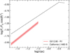 |
Fig. 7 Ratio of the centrifugal (Fc) and gravitational (Fg) forces in the R1 filament (red line), where θ represents the inclination angle of the filament relative to the POS. We assumed cos(θ) = 1, corresponding to a filament aligned with the POS. The red shaded area represents the lower limit error of 11 %, derived from the relative abundance uncertainty. For N2H+, the gravitational force dominates, with a distribution similar to the internal rotation observed in the California L1482-S filament (Álvarez-Gutiérrez et al. 2021). |
6 Discussion
Despite the morphological similarities between the two main G012 filaments, our analysis revealed differences in their gas kinematics, mass distributions, and core population. In the following discussion, we explore the different star-forming scenarios that may be associated with the R1 and R2 filaments and emphasize their potentially different evolutionary paths.
6.1 N2H+ destruction
In Sect. 3, we compared N2H+ emission with complementary tracers related to ionization, outflows, and dense gas in the G012 protocluster. Specifically, we highlighted a spatial anticorrelation between N2H+, C18O emission, and the H41α recombination line. Previously, Tobin et al. (2013) estimated the abundances of N2H+ in protostellar systems. In one of these systems (L1157), C18O traces regions without N2H+. Specifically, the authors found that as the C18O peaks decrease, N2H+ increases, indicating a clear anticorrelation between the two tracers. This anticorrelation was also detected by Tafalla et al. (2021), who also showed that N2H+ is detected at high column densities (N(H2) ≥ 1022 cm−2; see their Fig. 7). In addition, Yu et al. (2022) analyzed a H ``II``` bubble (S156) associated with the G305 star-forming complex and reported that N2H+ increased far to the edges of S156. This implies that N2H+ might be destroyed by the hot and expanding gas in the bubble. Together with increased CO near H ``II``` regions, the free electrons traced by recombination lines (e.g., H41α), ionized metal emission lines, and continuum emission provide additional methods for mapping these zones in which N2H+ is destroyed (e.g., Yu et al. 2018; Ginsburg et al. 2022b; Armante et al. 2024).
Galván-Madrid et al. (2024) analyzed the 3 mm continuum emission and H41α recombination line data for the full ALMAIMF sample and reported that an increase in emission is mostly seen in evolved regions with OB associations. All of these studies, along with the effect of temperature on the critical density of the N2H+ molecule (ranging from 6.1 × 104 cm−3 at 10 K to 2.0 × 104 cm−3 at 100 K), suggested a close relation between the decrease in N2H+ and the evolutionary stages of the protocluster. The critical density indicates the conditions under which N2H+ becomes an effective tracer, and they thus link its observed decrease to changes in the protocluster condition. In G012, the 1.3 mm continuum emission is concentrated at the center of the region and north of the R2 filament (see Fig. 1, right panel). Moreover, the 3 mm continuum exhibits high flux intensity distributions that appear as bubbles in the protocluster center (Ginsburg et al. 2022b), similar to the H41α distribution (bottom left panel of Fig. A.3). In addition, the relative N2H+ abundance distribution decreases in regions near H41α bubbles and ionizing emission from hot cores, highlighting the effect of feedback mechanisms in the distribution and abundance of the dense gas traced by N2H+. Because of the high concentrations of H41α and C18 O in the center of G012, it is likely that the central H ``II``` regions heat the gas in the protocluster and destroy the N2H+ molecule through interactions with free electrons (Vigren et al. 2012) and with the CO molecule (Bergin & Langer 1997; Caselli et al. 2002b; Caselli & Ceccarelli 2012).
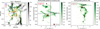 |
Fig. 8 DCN PV diagrams along the R2 filament and toward the central H ``II``` region. The left panel shows a zoom-in of the N2H+ moment 0 map, overlaid with DCN (green) and H41α (yellow) contours. The middle and right panels present DCN PV diagrams extracted from the red and brown boxes shown in the left panel, respectively. The red box highlights the filament extending toward the central H ``II``` bubble in the protocluster, and the brown box traces the R2 filament, including the northern region without N2H+ emission. The red stars indicate the cores detected in DCN (Cunningham et al. 2023). In the middle panel, the dashed black lines mark the center of the H ``II``` bubble (horizontal line) and the systemic velocity estimated from masers (Immer et al. 2014), corresponding to the approximate velocity of the H ``II``` bubble (37 km s−1 ; vertical line). |
6.2 DCN accretion evidence in the R2 filament and toward the central OB star cluster
As N2H+ is significantly affected by stellar feedback, particularly by the increase in temperature associated with the central massive OB star cluster, we further investigated the kinematics of the gas in these regions using DCN emission, which is more resilient to temperature enhancements. Although DCN does not trace filamentary structures as extended as those revealed by N2H+, it highlights hotter and denser gas components and reveals filamentary features within the R2 filament and in structures located close to the central OB cluster and the respective H ``II``` bubble.
First, we assessed whether the R2 filament showed evidence of ongoing core accretion processes. Recently, Dell'Ova et al. (2024) derived a dust temperature map of the G012 protocluster, finding values of ~35 K at the top of R2. They also reported a spatial shift between the H2 and N2H+ column density peaks, which they interpreted as the effect of a detected hot core (Armante et al. 2024) that heats the gas and destroys N2H+ at the top of the filament. The DCN emission in this region reveals a clear V-shaped structure. This feature was observed in other filaments undergoing accretion (e.g., Liu et al. 2019; Bonne et al. 2020, 2023; Álvarez-Gutiérrez et al. 2024; Sandoval-Garrido et al. 2025) and is coincident with the hot core location (see Fig. 8, right panel), along with an SiO-elongated feature perpendicular to the filament that is related to an outflow component (see Fig. 3 in Armante et al. 2024, and Fig. A.3). Additional kinematic evidence is found along the filament. Fig. 5 (right panel) shows that the average-velocity diagram reveals a clumping of velocities around ~1 km s−1 in the central and densest region of R2 that is spatially coincident with the integrated-intensity peak. Such clumps in PV space are commonly interpreted as signatures of accretion-driven core formation (e.g., Hacar et al. 2013; Kainulainen et al. 2016; Ladjelate et al. 2020), marking regions where gravity overcomes thermal support (e.g., André et al. 2010; Palau et al. 2013). Thus, the observed velocity clumping in addition to the small velocity spreads in the PV diagrams features along the R2 filament and the similar values in velocity between cores and dense gas further indicates an active role of cores in shaping the filament kinematics.
To place R2 in context, we compared its star-forming properties with those of the ISF OMC-2 filament. From previous catalogs (Megeath et al. 2012, Megeath et al. 2016; Furlan et al. 2016; Kainulainen et al. 2017; Stutz 2018; González Lobos & Stutz 2019), we derived an SFR of 95 M⊙ Myr−1 and an SFE of 0.008 for protostellar cores in OMC-2. In addition, previous studies estimated a line-mass profile of λ(ω) = 385 M⊙pc−1 (ω/pc)0.38 (Stutz 2018). Although the R2 line-mass profile is even steeper, its SFR is lower than that in OMC-2 (see Fig. 6), while both regions exhibit similar efficiencies. This comparison suggests that R2 is already in an evolved phase of filamentary accretion, possibly slightly earlier than OMC-2, but progressing toward a comparable state. This makes R2 an excellent candidate for testing filamentary accretion scenarios with upcoming James Webb Space Telescope (JWST) observations of YSOs in these filaments.
In addition to the accretion evidence identified in the R2 filament, we show in Fig. 8 a set of coherent velocity structures traced by DCN emission extending across the southern portion of R1 (blue box in the left panel) and toward the central region of the protocluster where the OB cluster is located (red box in the left panel). These structures appear as elongated features in DCN (green contours in the left panel) and display organized velocity patters in parallel PV diagrams toward the central region (middle panel). In particular, the parallel PV diagrams reveal multiple velocity gradients that form characteristic V-shaped patterns. While such V-shaped structures are often interpreted as signatures of gas inflow, we note that similar PV morphologies can arise from different kinematic configurations (e.g., rotation or outflows), and therefore do not uniquely trace accretion. One of these structures is detected toward the southern extended portion of the R1 filament (blue box). Here, DCN traces a relatively shallow V-shape that coincides spatially with a similar but weaker velocity pattern seen in the N2H+ emission. Unlike the more prominent structures discussed below, this feature does not appear to be directly associated with a compact core. This may indicate that the V-shaped structure traces gas motions along the filament that are not associated with a compact and localized gravitational potential (e.g., a prestellar or protostellar core, as observed in the R2 filament), and it might be consistent with large-scale gas flows along the southern portion of R1 that might include inflow.
More prominent V-shaped structures are observed closer to the central region of the cloud (red boxes). Specifically, we found two well-defined V-shaped patterns in DCN (see Fig. 8, middle panel), one of which appears to converge toward the position of a massive core detected in Cunningham et al. (2023). The coincidence of the vertex of the V-shaped and the location of the core suggests that this velocity gradient might trace gas flows feeding this object along the filamentary structure (Álvarez-Gutiérrez et al. 2024; Sandoval-Garrido et al. 2025). A second V-shaped velocity structure is detected nearby, whose vertex lies closer to the central region associated with the OB star cluster (represented by a horizontal dashed black line in the figure). The projected position of this feature is consistent with the location of one of the H ``II``` ionized bubbles in G012. While the spatial proximity to the ionized region raises the possibility that this observed gradient might be affected by stellar feedback, several observational characteristics suggest that it is more consistent with inflow motions than with outflowing gas. In particular, the relatively low velocity variations (around 4 km s−1) are significantly smaller than those typically observed in outflows, and the emission is traced by DCN, which probes cold and dense gas not usually associated with high-velocity ejected material. Together, these properties favor an interpretation in terms of gas motions directed toward the central H ``II``` region, possibly related to inflow, although contributions from feedback-induced perturbations or other complex velocity configurations cannot be entirely ruled out. We highlight that these types of patterns that connect R1 with the central region are not found for the R2 filament in N2H+ or DCN.
6.3 Potential star-forming scenarios in G012
The formation of stars occurs over diverse timescales, reflecting the intricate processes governing their evolution (Bergin & Tafalla 2007; Evans et al. 2009; Dunham & Vorobyov 2012; Dunham et al. 2014; Motte et al. 2018). These variations have direct implications for the G012 protocluster. In the R1 filament, which contains only two prestellar cores (Armante et al. 2024), the low SFR of ~4.24 M⊙ Myr−1 and an SFF of ~0.002 suggest that star formation is proceeding slowly despite the high gas density. In contrast, the R2 filament contains prestellar and protostellar cores and shows a significantly higher SFR of ~55.3 M⊙ Myr−1 and an SFF of ~0.008 (see Sect. 4.3). Although these estimates were derived from subregions (R1 and R2) selected to isolate the kinematically coherent portions of the filaments and not from their full spatial extent, the same trend is also observed for the larger scale structures (see Appendix B): the extended R1 filament still shows lower SFR and SFF values than the extended R2 filament.
The presence of multiple protostellar cores indicates that R2 has so far been more active in forming cores and is a more efficient star-forming region. The lack of protostellar cores and very limited number of prestellar cores in R1, together with the kinematic differences previously reviewed, show the marked contrasts between the two filaments. The differences suggest that R1 is at an earlier evolutionary stage, prior to the filament concentration and active star formation already evident in R2. This implies that, while potentially less evolved than R2, the R1 filament can eventually reach a higher level of core formation as its dense gas reservoir becomes more active. However, the physical processes driving this activity remain uncertain. Similar contrasts in core populations have also been reported in young filaments, such as those in the G351 protocluster (Sandoval-Garrido et al. 2025). However, the extended structure of R1 suggests that its internal evolutionary state might not be uniform. In particular, the lower portion of the filament, located closer to the central region hosting the OB star cluster and its associated H ``II``` bubbles, shows a higher concentration of dense cores and more complex kinematic signatures than the upper part of the R1 filament. The DCN PV diagrams reveal several V-shaped velocity patterns in the extended area at the bottom of R1, some of which converge toward massive cores, while others appear to be spatially connected to the central ionized region. These features might trace localized gas inflows along filamentary structures toward either individual cores or the cluster environment. One possible interpretation is that the expansion of the nearby H ``II``` bubble compresses the surrounding molecular gas, potentially enhancing core formation in the lower portion of R1. Such feedback-driven triggering has been suggested in other star-forming regions where expanding ionized bubbles interact with dense filaments (e.g., Arzoumanian et al. 2022; Neupane et al. 2024). In this context, the higher abundance of dense cores in this bottom and extend part of R1 might reflect a locally accelerated phase of star formation (compared to the upper part, which exhibits potential rotation signatures) superposed on an otherwise less evolved filament.
Additional evidence supporting this evolutionary contrast comes from chemical differentiation in other regions where molecular tracers such as DCN and N2D+ highlight different physical conditions (e.g., Sakai et al. 2022; Cunningham et al. 2023), suggesting that similar mechanisms might be at play in G012. Moreover, the estimated lifetimes of high-mass prestellar cores in Valeille-Manet et al. (2025) are comparable to the velocity gradient timescale in R1 (~0.1 Myr), suggesting that the observed kinematic conditions might set a characteristic timescale for core formation. This supports a causal view where gas kinematics drive core assembly and evolution and do not simply result from it. However, this interpretation likely applies primarily to the filament regions that are not strongly affected by external feedback. In the lower part of the extended R1 structure (the region traced by DCN), which lies closer to the central H ``II``` region, the gas kinematics might also be affected by the expansion of the ionized bubble, which might modify the local conditions for core formation (see above). The contrasting core populations and timescales in R1 and R2 thus highlight how local dynamical conditions regulate the star formation efficiency and rate. Comparisons with other regions reinforce this evolutionary interpretation. As shown in Fig. 9, the PV-diagram features and line-mass profiles of R1 and R2 resemble those of filaments at different stages: R1 shares characteristics with the early-stage quiescent L1482-S region (Álvarez-Gutiérrez et al. 2021), while R2 resembles the more evolved Orion ISF (González Lobos & Stutz 2019). For this comparison to be meaningful, it is important to verify that the datasets probe similar physical and kinematics scales. Although the angular resolutions differ among the above mentioned datasets, the physical resolutions are comparable. The N2H+ observations of González Lobos & Stutz (2019) and Álvarez-Gutiérrez et al. (2021) have spatial resolutions of 17–22" at distances of 420–500 pc, corresponding to 7–11 kau, respectively. Our observations have a beam of 2.3" at 2.4 kpc, corresponding to 6 kau. Therefore, all datasets probe similar physical scales along the filaments. The spectral resolution in our data (0.23 km s−1) is moderately higher than in those studies (0.12-0.16 km s−1), which might smooth very fine velocity substructure but does not affect the identification of global velocity gradients or velocity spread features discussed here.
The coexistence of filaments in distinct evolutionary phases within the same protocluster has been observed in other regions (e.g., Tafalla et al. 2004; André et al. 2010; Schneider et al. 2012; Hacar et al. 2013; Peretto et al. 2014; Zhou et al. 2022; Sandoval-Garrido et al. 2025). For instance, in the Taurus cloud, Hacar et al. (2013) identified coherent filaments exhibiting quiescent and active regions. Similar findings were reported in SDC13 (Peretto et al. 2014) and the Rosette cloud (Schneider et al. 2012), where filaments with different densities, temperatures, and fragmentation levels coexist. Several factors can explain this diversity, including initial density variations, differential gas accretion, and local feedback from protostellar outflows and H ``II```. Denser filaments tend to collapse earlier, while diffuse structures can remain stable or be affected by nearby activity. These mechanisms can lead to asynchronous star formation, where young stellar objects in the same cluster span a wide range of ages (Peretto et al. 2014; Nony et al. 2021). Recognizing the presence of filaments at different stages within a single region like G012 is key to understanding the temporal and spatial complexity of star formation in protoclusters. An intriguing open question is whether the apparent rotation of R1 reflects a genuine large-scale rotational motion with potential inherited angular momentum from the parent molecular cloud or arises from other kinematic configurations. Several alternative scenarios can produce apparent transverse velocity gradients. We list the scenarios below.
A coherent rotation of the filament would naturally produce a smooth and approximately linear velocity gradient perpendicular to the filament ridge line. This behavior is indeed observed in the R1 filament, where the ridge line-averaged velocity versus radius diagram reveals a well-defined and continuous gradient (Fig. 5, left panel);
The observed gradient might result from unresolved dense substructures, such as fibers, forming cores, or accretion streamers. Simulations and observations suggest that young filaments can retain rotational signatures from their fragmentation process, with cores often exhibiting rotation axes preferentially aligned relative to the filament orientation (Kong et al. 2019; Hsieh et al. 2021; Lee et al. 2025). Alternatively, sub-filamentary networks such as fibers and streamers that are common in turbulent clouds can serve as conduits for organized flows and potentially impart angular momentum to host filaments (Hacar et al. 2017; Maud et al. 2017; Hacar et al. 2018; Pineda et al. 2023; Olguin et al. 2025). In this case, we would expect a more fragmented velocity structure, with discontinuities or localized deviations along the filament. While such substructures may be present below the current angular resolution, the smoothness of the averaged gradient in the top of R1 suggests that they do not dominate the large-scale kinematics;
Organized inflows of gas along sub-filamentary networks can also imprint velocity gradients. These flows typically produce asymmetric or localized velocity patterns such as V-shaped structures in parallel PV diagrams. In R1, we analyzed parallel gradients, but found no V-shaped structures in the region that exhibits the proposed rotation feature. We only found a weaker V-shaped pattern that is detected in the bottom extended portion of R1 traced by DCN and N2H+, and near the central H ``II``` region. This might suggest localized inflows toward the central H ``II``` bubble environment rather than along the entire filament (Fig. 8, middle panel);
External feedback, such as the expansion of nearby H ``II``` regions, might strongly perturb filament kinematics by compressing gas and enhancing velocity dispersions (Zhou et al. 2022; Arzoumanian et al. 2022; Neupane et al. 2024; Zhao et al. 2025). Although these effects can contribute locally, the absence of a comparable transverse gradient in the nearby R2 filament, which lies within the same large-scale environment, suggests that feedback alone cannot explain the kinematic behavior observed in R1.
Of the possible explanations, a coherent rotation of the filament provides the most straightforward interpretation of the observed transverse velocity gradient. While localized inflows or feedback-related perturbations can contribute to the kinematics in specific regions, particularly in the bottom and extended portion of R1 near to the H ``II``` region, the overall smoothness and continuity of the transverse gradient along the filament are most consistent with large-scale rotational motion. Separating these other alternative scenarios requires higherresolution observations capable of resolving sub-parsec structures such as fibers, forming cores, and accretion streamers, and detailed comparisons with simulations of feedback-affected filaments.
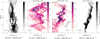 |
Fig. 9 Comparative PV diagrams of California L1482-south (left panel, Álvarez-Gutiérrez et al. 2021), OMC-2 (right panel, González Lobos & Stutz 2019), and the R1 and R2 filaments (center panels). Similar to California, R1 presents a double-helix feature, low presence of cores, and low temperatures (<25 K, see Dell'Ova et al. 2024). Despite this, line-mass profile of both regions (estimated within the range of the red lines on the central panels) shows that R1 is more massive and dense than California L1482-south. Furthermore, R2 shows PV diagram features comparable to the ISF OMC-2 region. Specifically, R2 presents smooth undulations in velocities characterized with uniform velocities. R2 is also characterized by a high presence of cores. |
7 Conclusions
G012 is one of the most evolved and massive regions in the ALMA-IMF protocluster sample. Its dense gas emission, traced by the N2H+ molecule, reveals a morphology mainly composed of two large filaments, and additional irregular but similarly dense structures. The center of G012 presents an absence of N2H+, which agrees with the existence of large-scale H ``II``` regions, which destroys the dense gas that forms a disrupted structure in the protocluster center. We focused on the kinematical analysis of the N2H+ emission of the G012 protocluster, including a line-mass distribution analysis, and the kinematic characterization of its two main filamentary structures, which we named R1 and R2. Our main conclusions are summarized below:
We found multiple velocity components in G012. About 55% of the N2H+ spectra are well fitted by two velocity components, and the remainder are well described by a single velocity component. We defined the two main velocity structures in the protocluster as the first and second velocity components, FVC and SVC, respectively;
The integrated-intensity map revealed two dominant filamentary structures: the R1 and R2 filaments. Despite their similarity in morphology, we found obvious differences in their kinematics;
R1 is characterized by a velocity gradient across its spine in the moment 1 map. We review the PV diagram features, which showed a helical structure at the top of the filament that might be associated with filament rotation. We found an average velocity gradient of ~ 10.4 km s−1 pc−1 (or ~0.1 Myr timescale) in this feature;
R2 is characterized by smooth, compact velocity undulations (<2 km s−1) and the absence of a large-scale velocity gradient;
The mean line-mass profiles of the two filaments are well described by λ(ω) = 5660 M⊙ pc−1 (ω/pc)0.30 and λ(ω) = 6943 M⊙ pc−1 (ω/pc)0.20 for R1 and R2, respectively. When we compared these distributions with those from other well-studied regions, we found that R1 and R2 stand out as having significantly higher line-mass profiles, which is consistent with higher densities than the structures mentioned above. Based on these line-mass profiles, we calculated the gravitational field, force, and potential for R1 and R2, assuming cylindrical symmetry;
Using simple toy models, we estimated in R1 the ratio of the centrifugal to gravitational force (the latter based on the line-mass profile). We found that rotation in the R1 filament is subdominant compared to gravity, but as the radius increases, the role of rotation increases. This is very similar to the behavior reported for the California L1482 filament (Álvarez-Gutiérrez et al. 2021);
While the kinematic features appear to be similar between L1482 and R1, the line-mass profile normalization at 1 pc of R1 is almost 30 times higher than that of L1482. Hence, the similarities in the kinematics and the force-ratio profiles might indicate a common angular momentum evolution of filaments across wide ranges in mass and line-mass scales;
In terms of the estimated star formation activity, R1 lacks protostellar cores, and the few cores that are present are in the prestellar phase, implying an SFR ~ 4.24 M⊙ Myr−1. In contrast, R2 hosts a larger population of massive cores than R1 and contains an SiO outflow oriented perpendicular to the filament. Specifically, R2 forms protostellar cores at a rate of SFR ~ 55.3 M⊙ Myr−1 with a similar efficiency as the Orion ISF;
We identified filamentary structures traced by DCN exhibiting signatures of potential accretion toward the center of the protocluster, where the OB stellar cluster is located and N2H+ is largely destroyed, suggesting that these structures might represent the remnants of a former hub-filament system;
Using N2H+ (1−0) and DCN (3−2) spectral lines, we estimated updated velocities for 48 previously identified cores. In general, the cores appear to be kinematically coupled to the dense gas traced by N2H+ and DCN from which they are forming;
Considering the differences of R1 versus R2 in gas kinematics, core incidence, and estimated SFRs, we proposed that R1 is still rotating and younger than the R2 filament, which has collapsed to a more efficient mode of star formation, likely by shedding its angular momentum.
The results we presented emphasize the role of dense filamentary structures in high-mass star formation, especially when found at different stages of evolution within the same protocluster. The detection of filaments in different evolutionary phases within a single protocluster allowed us to characterize multiple stages of star formation, from the earliest accretion processes to later stages of core collapse, but after feedback effects from H ``II``` regions. By uncovering these structures, we gained valuable insights into the diverse mechanisms governing the gas kinematics, including gas accretion and filament rotation evolution. This ability to observe a snapshot of the different stages in one region presents a unique window into the ongoing processes shaping Milky Way protoclusters.
Acknowledgements
ADS/JAO.ALMA#2017.1.01355.L. ALMA is a partnership of ESO (representing its member states), NSF (USA) and NINS (Japan), together with NRC (Canada), MOST and ASIAA (Taiwan), and KASI (Republic of Korea), in cooperation with the Republic of Chile. The Joint ALMA Observatory is operated by ESO, AUI/NRAO and NAOJ. The project leading to this publication has received support from ORP, which is funded by the European Union's Horizon 2020 research and innovation program under grant agreement No. 101004719 [ORP]. A.S., J.S., N.S.G., R.A.G., N.C.T., and G.B.M. gratefully acknowledge support by the Fondecyt Regular (project code 1220610), and ANID BASAL project FB210003. R.G.M. and J.S. acknowledge support from UNAM-DGAPA-PAPIIT project IN105225. R.A.G. gratefully acknowledges support from ANID Beca Doctorado Nacional 21200897. F.L. and F.M. acknowledge funding from the European Research Council (ERC) via the ERC Synergy Grant ECOGAL (grant 855130) and from the French Agence Nationale de la Recherche (ANR) through the project COSMHIC (ANR-20-CE31-0009). A.K. gratefully acknowledges support from Fondecyt postdoctoral grant. L.B. gratefully acknowledges support by the ANID BASAL project FB210003. N.S.G. gratefully acknowledges support from ANID Beca Doctorado Nacional 21250244. G.B. acknowledges support from the PID2023-146675NB-I00 (MCI-AEI-FEDER, UE) program.
References
- Álvarez-Gutiérrez, R. H., Stutz, A. M., Law, C. Y., et al. 2021, ApJ, 908, 86 [CrossRef] [Google Scholar]
- Álvarez-Gutiérrez, R. H., Stutz, A. M., Sandoval-Garrido, N., et al. 2024, A&A, 689, A74 [NASA ADS] [CrossRef] [EDP Sciences] [Google Scholar]
- André, P., Men'shchikov, A., Bontemps, S., et al. 2010, A&A, 518, L102 [CrossRef] [EDP Sciences] [Google Scholar]
- André, P., Di Francesco, J., Ward-Thompson, D., et al. 2014, Protostars and Planets VI, 27 [Google Scholar]
- Armante, M., Gusdorf, A., Louvet, F., et al. 2024, A&A, 686, A122 [NASA ADS] [CrossRef] [EDP Sciences] [Google Scholar]
- Arzoumanian, D., Russeil, D., Zavagno, A., et al. 2022, A&A, 660, A56 [NASA ADS] [CrossRef] [EDP Sciences] [Google Scholar]
- Bergin, E. A. & Langer, W. D., 1997, ApJ, 486, 316 [Google Scholar]
- Bergin, E. A., & Tafalla, M. 2007, ARA&A, 45, 339 [Google Scholar]
- Bonfand, M., Csengeri, T., Bontemps, S., et al. 2024, A&A, 687, A163 [NASA ADS] [CrossRef] [EDP Sciences] [Google Scholar]
- Bontemps, S., Motte, F., Csengeri, T., et al. 2010, A&A, 524, A18 [NASA ADS] [CrossRef] [EDP Sciences] [Google Scholar]
- Bonne, L., Bontemps, S., Schneider, N., et al. 2020, A&A, 644, A27 [EDP Sciences] [Google Scholar]
- Bonne, L., Bontemps, S., Schneider, N., et al. 2023, ApJ, 951, 39 [CrossRef] [Google Scholar]
- Busquet, G., Estalella, R., Zhang, Q., et al. 2011, A&A, 525, A141 [NASA ADS] [CrossRef] [EDP Sciences] [Google Scholar]
- CASA Team (Bean, B., et al.) 2022, PASP, 134, 114501 [NASA ADS] [CrossRef] [Google Scholar]
- Caselli, P., & Ceccarelli, C. 2012, A&A Rev., 20, 56 [NASA ADS] [Google Scholar]
- Caselli, P., Myers, P. C., & Thaddeus, P. 1995, ApJ, 455, L77 [Google Scholar]
- Caselli, P., Walmsley, C. M., Zucconi, A., et al. 2002a, ApJ, 565, 344 [Google Scholar]
- Caselli, P., Walmsley, C. M., Zucconi, A., et al. 2002b, ApJ, 565, 331 [NASA ADS] [CrossRef] [Google Scholar]
- Caselli, P., Benson, P. J., Myers, P. C., et al. 2002c, ApJ, 572, 238 [CrossRef] [Google Scholar]
- Csengeri, T., Bontemps, S., Schneider, N., et al. 2011a, A&A, 527, A135 [NASA ADS] [CrossRef] [EDP Sciences] [Google Scholar]
- Csengeri, T., Bontemps, S., Schneider, N., et al. 2011b, ApJ, 740, L5 [NASA ADS] [CrossRef] [Google Scholar]
- Csengeri, T., Bontemps, S., Wyrowski, F., et al. 2017, A&A, 601, A60 [NASA ADS] [CrossRef] [EDP Sciences] [Google Scholar]
- Cunningham, N., Ginsburg, A., Galván-Madrid, R., et al. 2023, A&A, 678, A194 [NASA ADS] [CrossRef] [EDP Sciences] [Google Scholar]
- Dell'Ova, P., Motte, F., Gusdorf, A., et al. 2024, A&A, 687, A217 [NASA ADS] [CrossRef] [EDP Sciences] [Google Scholar]
- Duarte-Cabral, A., Bontemps, S., Motte, F., et al. 2013, A&A, 558, A125 [NASA ADS] [CrossRef] [EDP Sciences] [Google Scholar]
- Dunham, M. M., & Vorobyov, F. I. 2012, ApJ, 747, 52 [NASA ADS] [CrossRef] [Google Scholar]
- Dunham, M. M., Stutz, A. M., Allen, L. F., et al. 2014, Protostars and Planets VI, 195 [Google Scholar]
- Evans, N. J., Dunham, M. M., Jørgensen, J. K., et al. 2009, ApJS, 181, 321 [NASA ADS] [CrossRef] [Google Scholar]
- Fndres, C. P., Schlemmer, S., Schilke, P., et al. 2016, arXiv e-prints [arXiv:1603.03264] [Google Scholar]
- Friesen, R. K., Di Francesco, J., Myers, P. C., et al. 2010, ApJ, 718, 666 [NASA ADS] [CrossRef] [Google Scholar]
- Furlan, F., Fischer, W. J., Ali, B., et al. 2016, ApJS, 224, 5 [Google Scholar]
- Galván-Madrid, R., Zhang, Q., Keto, F., et al. 2010, ApJ, 725, 17 [NASA ADS] [CrossRef] [Google Scholar]
- Galván-Madrid, R., Díaz-González, D. J., Motte, F., et al. 2024, ApJS, 274, 15 [CrossRef] [Google Scholar]
- Ginsburg, A., Csengeri, T., Galván-Madrid, R., et al. 2022, A&A, 662, A9 [NASA ADS] [CrossRef] [EDP Sciences] [Google Scholar]
- Ginsburg, A., Sokolov, V., de Val-Borro, M., et al. 2022, AJ, 163, 291 [NASA ADS] [CrossRef] [Google Scholar]
- González Lobos, V., & Stutz, A. M. 2019, MNRAS, 489, 4771 [CrossRef] [Google Scholar]
- Gómez, G. C., Walsh, C., & Palau, A. 2022, MNRAS, 513, 1244 [CrossRef] [Google Scholar]
- Hacar, A., & Tafalla, M. 2011, A&A, 533, A34 [NASA ADS] [CrossRef] [EDP Sciences] [Google Scholar]
- Hacar, A., Tafalla, M., Kauffmann, J., et al. 2013, A&A, 554, A55 [NASA ADS] [CrossRef] [EDP Sciences] [Google Scholar]
- Hacar, A., Tafalla, M., & Alves, J. 2017, A&A, 606, A123 [NASA ADS] [CrossRef] [EDP Sciences] [Google Scholar]
- Hacar, A., Tafalla, M., Forbrich, J., et al. 2018, A&A, 610, A77 [NASA ADS] [CrossRef] [EDP Sciences] [Google Scholar]
- Hacar, A., Clark, S. F., Heitsch, F., et al. 2023, Protostars and Planets VII, 534, 153 [NASA ADS] [Google Scholar]
- Haschick, A. D., & Ho, P. T. P. 1983, ApJ, 267, 638 [Google Scholar]
- Hsieh, C.-H., Arce, H. G., Mardones, D., et al. 2021, ApJ, 908, 92 [CrossRef] [Google Scholar]
- Immer, K., Reid, M. J., Menten, K. M., et al. 2013, A&A, 553, A117 [NASA ADS] [CrossRef] [EDP Sciences] [Google Scholar]
- Immer, K., Galvân-Madrid, R., König, C., et al. 2014, A&A, 572, A63 [NASA ADS] [CrossRef] [EDP Sciences] [Google Scholar]
- Jessop, N. F., & Ward-Thompson, D. 2000, MNRAS, 311, 63 [NASA ADS] [CrossRef] [Google Scholar]
- Kainulainen, J., Hacar, A., Alves, J., et al. 2016, A&A, 586, A27 [NASA ADS] [CrossRef] [EDP Sciences] [Google Scholar]
- Kainulainen, J., Stutz, A. M., Stanke, T., et al. 2017, A&A, 600, A141 [NASA ADS] [CrossRef] [EDP Sciences] [Google Scholar]
- Kirk, H., Myers, P. C., Bourke, T. L., et al. 2013, ApJ, 766, 115 [Google Scholar]
- Koch, F. W., & Rosolowsky, F. W. 2016, Astrophysics Source Code Library [record ascl:1608.009] [Google Scholar]
- Koley, A., Stutz, A. M., Louvet, F., et al. 2025, A&A, 702, A133 [NASA ADS] [CrossRef] [EDP Sciences] [Google Scholar]
- Kong, S., Arce, H. G., Maureira, M. J., et al. 2019, ApJ, 874, 104 [Google Scholar]
- Könyves, V., André, P., Men'shchikov, A., et al. 2015, A&A, 584, A91 [NASA ADS] [CrossRef] [EDP Sciences] [Google Scholar]
- Ladjelate, B., André, P., Könyves, V., et al. 2020, A&A, 638, A74 [NASA ADS] [CrossRef] [EDP Sciences] [Google Scholar]
- Lee, H.-T., Tang, Y.-W., Koch, P. M., et al. 2025, A&A, 696, A163 [NASA ADS] [CrossRef] [EDP Sciences] [Google Scholar]
- Lippok, N., Launhardt, R., Semenov, D., et al. 2013, A&A, 560, A41 [NASA ADS] [CrossRef] [EDP Sciences] [Google Scholar]
- Liu, H.-L., Stutz, A., & Yuan, J.-H. 2019, MNRAS, 487, 1259 [Google Scholar]
- Liu, H.-L., Tej, A., Liu, T., et al. 2023, MNRAS, 522, 3719 [NASA ADS] [CrossRef] [Google Scholar]
- Louvet, F., Sanhueza, P., Stutz, A., et al. 2024, A&A, 690, A33 [NASA ADS] [CrossRef] [EDP Sciences] [Google Scholar]
- Maud, L. T., Hoare, M. G., Galván-Madrid, R., et al. 2017, MNRAS, 467, L120 [NASA ADS] [Google Scholar]
- Megeath, S. T., Gutermuth, R., Muzerolle, J., et al. 2012, AJ, 144, 192 [NASA ADS] [CrossRef] [Google Scholar]
- Megeath, S. T., Gutermuth, R., Muzerolle, J., et al. 2016, AJ, 151, 5 [Google Scholar]
- Megeath, S. T., Gutermuth, R. A., & Kounkel, M. A. 2022, PASP, 134, 042001 [CrossRef] [Google Scholar]
- Men'shchikov, A. 2021, A&A, 649, A89 [NASA ADS] [CrossRef] [EDP Sciences] [Google Scholar]
- Merín, B., Jørgensen, J., Spezzi, L., et al. 2008, ApJS, 177, 551 [Google Scholar]
- Motte, F., Bontemps, S., & Louvet, F. 2018, ARA&A, 56, 41 [Google Scholar]
- Motte, F., Bontemps, S., Csengeri, T., et al. 2022, A&A, 662, A8 [NASA ADS] [CrossRef] [EDP Sciences] [Google Scholar]
- Motte, F., Pouteau, Y., Nony, T., et al. 2025, A&A, 694, A24 [NASA ADS] [CrossRef] [EDP Sciences] [Google Scholar]
- Neupane, S., Wyrowski, F., Menten, K. M., et al. 2024, A&A, 692, A114 [NASA ADS] [CrossRef] [EDP Sciences] [Google Scholar]
- Nony, T., Robitaille, J.-F., Motte, F., et al. 2021, A&A, 645, A94 [NASA ADS] [CrossRef] [EDP Sciences] [Google Scholar]
- Nony, T., Galván-Madrid, R., Motte, F., et al. 2023, A&A, 674, A75 [NASA ADS] [CrossRef] [EDP Sciences] [Google Scholar]
- Olguin, F. A., Sanhueza, P., Ginsburg, A., et al. 2025, Sci. Adv., 11, 34, eadw4512 [Google Scholar]
- Padoan, P., & Nordlund, Å. 2002, ApJ, 576, 870 [NASA ADS] [CrossRef] [Google Scholar]
- Palau, A., Fuente, A., Girart, J. M., et al. 2013, ApJ, 762, 120 [NASA ADS] [CrossRef] [Google Scholar]
- Peretto, N., Fuller, G. A., André, P., et al. 2014, A&A, 561, A83 [NASA ADS] [CrossRef] [EDP Sciences] [Google Scholar]
- Pineda, J. F., Arzoumanian, D., André, P., et al. 2023, Protostars and Planets VII, 534, 233 [NASA ADS] [Google Scholar]
- Pouteau, Y., Motte, F., Nony, T., et al. 2022, A&A, 664, A26 [NASA ADS] [CrossRef] [EDP Sciences] [Google Scholar]
- Pouteau, Y., Motte, F., Nony, T., et al. 2023, A&A, 674, A76 [NASA ADS] [CrossRef] [EDP Sciences] [Google Scholar]
- Punanova, A., Caselli, P., Pon, A., et al. 2016, A&A, 587, A118 [NASA ADS] [CrossRef] [EDP Sciences] [Google Scholar]
- Redaelli, F., Bizzocchi, L., Caselli, P., et al. 2019, A&A, 629, A15 [NASA ADS] [CrossRef] [EDP Sciences] [Google Scholar]
- Reyes-Reyes, S. D., Stutz, A. M., Megeath, S. T., et al. 2024, MNRAS, 529, 2220 [NASA ADS] [CrossRef] [Google Scholar]
- Sabatini, G., Bovino, S., Sanhueza, P., et al. 2022, ApJ, 936, 80 [NASA ADS] [CrossRef] [Google Scholar]
- Sandoval-Garrido, N. A., Stutz, A. M., Álvarez-Gutiérrez, R. H., et al. 2025, A&A, 696, A202 [NASA ADS] [CrossRef] [EDP Sciences] [Google Scholar]
- Sakai, T., Sanhueza, P., Furuya, K., et al. 2022, ApJ, 925, 144 [NASA ADS] [CrossRef] [Google Scholar]
- Schneider, N., Csengeri, T., Hennemann, M., et al. 2012, A&A, 540, L11 [NASA ADS] [CrossRef] [EDP Sciences] [Google Scholar]
- Shirley, Y. L. 2015, PASP, 127, 299 [Google Scholar]
- Stutz, A. M. 2018, MNRAS, 473, 4890 [NASA ADS] [CrossRef] [Google Scholar]
- Stutz, A. M., & Gould, A. 2016, A&A, 590, A2 [NASA ADS] [CrossRef] [EDP Sciences] [Google Scholar]
- Stutz, A. M., Gonzalez-Lobos, V., & Gould, A. 2018, arXiv e-prints [arXiv:1807.11496] [Google Scholar]
- Tafalla, M., Santiago, J., Johnstone, D., et al. 2004, A&A, 423, L21 [NASA ADS] [CrossRef] [EDP Sciences] [Google Scholar]
- Tanaka, T., Nakamura, F., Awazu, Y., et al. 2013, ApJ, 778, 34 [NASA ADS] [CrossRef] [Google Scholar]
- Tafalla, M., Usero, A., & Hacar, A. 2021, A&A, 646, A97 [NASA ADS] [CrossRef] [EDP Sciences] [Google Scholar]
- Tatematsu, K., Kandori, R., Umemoto, T., et al. 2008, PASJ, 60, 407 [Google Scholar]
- Thaddeus, P., & Turner, B. F. 1975, ApJ, 201, L25 [Google Scholar]
- Tobin, J. J., Bergin, F. A., Hartmann, L., et al. 2013, ApJ, 765, 18 [NASA ADS] [CrossRef] [Google Scholar]
- Towner, A. P. M., Ginsburg, A., Dell'Ova, P., et al. 2024, ApJ, 960, 48 [NASA ADS] [CrossRef] [Google Scholar]
- Valeille-Manet, M., Bontemps, S., Csengeri, T., et al. 2025, A&A, 696, A11 [NASA ADS] [CrossRef] [EDP Sciences] [Google Scholar]
- Vázquez-Semadeni, F., Palau, A., Ballesteros-Paredes, J., et al. 2019, MNRAS, 490, 3061 [CrossRef] [Google Scholar]
- Vigren, F., Zhaunerchyk, V., Hamberg, M., et al. 2012, ApJ, 757, 34 [NASA ADS] [CrossRef] [Google Scholar]
- Xie, J., Li, J., Wang, J., et al. 2023, ApJ, 949, 89 [Google Scholar]
- Xu, F.-W., Wang, K., Liu, T., et al. 2023, MNRAS, 520, 3259 [NASA ADS] [CrossRef] [Google Scholar]
- Yu, N.-P., Xu, J.-L., Wang, J.-J., et al. 2018, ApJ, 865, 135 [NASA ADS] [CrossRef] [Google Scholar]
- Yu, N., Wang, J.-J., & Xu, J.-L. 2019, MNRAS, 489, 4497 [CrossRef] [Google Scholar]
- Yu, N.-P., Xu, J.-L., Zhang, C.-P., et al. 2022, ApJ, 928, 83 [Google Scholar]
- Zhou, J.-W., Liu, T., Fvans, N. J., et al. 2022, MNRAS, 514, 6038 [NASA ADS] [CrossRef] [Google Scholar]
- Zhao, M., Tang, X., Qiu, K., et al. 2025, A&A, 696, A178 [NASA ADS] [CrossRef] [EDP Sciences] [Google Scholar]
Proposal ID 2017.1.01355.L. ALMA-IMF aims to probe the origin of the IMF in our Galaxy, providing unprecedented multi-scale data on cores, filaments, and chemically rich regions. This LP focuses on a variety of separate but related topics and techniques, such as the analysis of the different populations of cores in the sample (e.g., Cunningham et al. 2023; Pouteau et al. 2022, 2023; Nony et al. 2023; Louvet et al. 2024; Motte et al. 2025), search for chemically rich regions using complex organic molecules (e.g., Bonfand et al. 2024; Armante et al. 2024), study of outflows (e.g., Towner et al. 2024; Valeille-Manet et al. 2025), and also (but not exclusively) gas kinematics in dense filaments (e.g., Álvarez-Gutiérrez et al. 2024; Sandoval-Garrido et al. 2025).
We consider the timescale  , neglecting projection effects and assuming a linear velocity gradient, where v is the velocity axis and p the position axis in the PV.
Appendix A N2H+ (1−0) line fitting: one and two velocity components
In this appendix, we describe the data preparation steps prior to line fitting, including S/N analysis and input parameter selection. We also characterize the output modeling parameters and associated uncertainties, identifying the velocity structures used in the above analysis.
Appendix A.1 Data preparation
Before fitting, we evaluate the robustness of the N2H+ data cube by inspecting negative bowls and noise levels. The most negative values are concentrated toward the compact central region of G012. To identify reliable spectra, we construct an S/N map, where the noise is estimated pixel-by-pixel from the RMS in emission-free channels between 12-20 km s−1 and 49–61 km s−1. The S/N ratio is defined as the peak intensity per pixel divided by its RMS noise. We adopt an S/N threshold of 12, preserving most of the N2H+ structure while excluding noisy or unresolved spectra unsuitable for fitting. Preliminary moment 0 and 1 maps are constructed using the full line for the integrated-intensity and the isolated component for the mean velocity (see Álvarez-Gutiérrez et al. 2024, for details on isolated component identification). The integrated-intensity map (right panel in Fig. 1) reveals two main N2H+ filaments and a disrupted central morphology in G012. The moment 1 map shows a velocity gradient perpendicular to the R1 filament ridge line (Sect. 4.1) and broad velocity dispersion in the central region, likely associated with multiple velocity components.
Appendix A.2 Choosing input parameters
To model the N2H+ data, we used the specfit fitting tool based on the built-in n2hp_vtau fitter. The specfit task requires the following input values: fittype specifies the model type and requires the number of velocity components and model parameters; guesses are initial model parameter values (only applied to the first pixel fit); limits are lower and upper parameter bounds used across all pixels via the Levenberg-Marquardt algorithm optimizing the χ2 function; limited applies or disregards the limits defined above; errmap is the error map, calculated as the standard deviation in the noise channels (see above); signal_cut defines the signal lower limit for the modeling, where S/N > signal_cut; and start_from_point is the initial pixel for fitting.
We test models with one and two velocity components, using four main parameters: the excitation temperature (Tex), optical depth (τ), velocity centroid (Vc), and velocity dispersion (σ). For the initial guesses and limits, we select values based on the preliminary moment maps described above. The start_from_point is chosen as a pixel with high S/N and a well-defined spectrum. Testing various signal_cut values confirms that pixels below an S/N of 12 yield poor fits or large uncertainties in critical parameters like radial velocities errors. The input parameters for one- and two-component fits are listed in Table A.1.
Appendix A.3 Output parameters and dependencies
PySpecKit produces cubes containing the best-fit parameters (Tex, τ, Vc, and σ) and their associated uncertainties for each spectrum and velocity component. Using these parameters, we construct a modeled N2H+ cube and separate the first (FVC) and second (SVC) velocity components into individual cubes. To evaluate the dependence of the fitting on the input parameters, we analyze the two most prominent N2H+ filaments (R1 and R2; Fig. 1). We test the start_pixel parameter while keeping all other inputs fixed, performing 716 fits for R1 and 576 for R2, each using a different initial pixel. We find that the derived parameters and uncertainties are largely independent of the initial pixel. However, when fitting multiple velocity components, the starting pixel must correspond to a spectrum where the components are clearly resolved. We also test different parameter limits and find that our adopted ranges are sufficiently broad to avoid biasing the results.
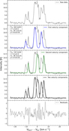 |
Fig. A.1 N2H+ two velocity component fitting example: The panels, from top to bottom, display the raw data (grey curve), the first velocity component (blue curve) overlaid on the raw data, the second velocity component (green curve) overlaid on the raw data, the total model (black curve) fitted to the raw data, and the residuals of the model (grey dashed curve). The PySpecKit parameters for the first and second velocity components are shown in each respective panel. |
Appendix A.4 Output cleaning
With this modeling approach, some spectra may yield poor fits due to noise or an incorrect number of velocity components. Therefore, it is essential to identify the appropriate number of components and assess the quality of the fitted parameters and uncertainties. In particular, we analyze the error distributions of the fitted parameters. Errors in centroid velocity and velocity dispersion are mostly below 0.3 km s−1, with only 5 and 26 pixels exceeding this value, respectively. Since this threshold is conservative relative to the N2H+ velocity resolution, we adopt it as the maximum allowed uncertainty for Vc and σ. We also find 184 fits with σ uncertainties equal to 0 km s−1, indicating that the best-fit values lie at the edge of the allowed parameter range. These spectra likely contain unresolved velocity structure and may require multiple velocity components.
Starting guesses for spectral fitting
The parameter τ is more difficult to constrain because it can become arbitrarily large. We therefore apply a mask requiring τ/e(τ) > 1, where e(τ) is the uncertainty in τ. Large τ values are typically associated with large uncertainties and flat-top spectral profiles, leading us to exclude ~860 pixels from the model. Most retained τ values are below 25. For Tex, optically thin pixels (τ < 1) often converge to the upper input limit with uncertainties of 0 K. However, because Tex has little impact on the spectral profile in this regime, we retain the original fitted values until the column density analysis (Sect. 3.3).
Inspection of the rejected spectra shows that many are associated with multiple velocity components, including cases where the components are difficult to resolve. To address this, we refit the entire cube using two velocity components and evaluate whether the fits improve inside and outside the previous selection criteria. For spectra containing a single velocity component, the two-component model often produces poor fits for either the bluest or reddest component. In these cases, we retain the single-component fit when its uncertainties are low and the fit quality is satisfactory. In addition, poor two-component fits are generally associated with velocity uncertainties larger than 0.3 km s−1 (~15% of pixels), large relative τ uncertainties (~30%), zero-valued parameters (11% of pixels), and high τ values. We additionally impose an upper limit of τ = 100 for each velocity component, removing 52 pixels above this threshold.
In total, we obtain ~15 000 spectra with a well defined model for one (~45%) or two (~55%) velocity components. Two velocity components are spatially distributed in the whole region, without a preferred location, but with a slight concentration in the R2 filament and in regions with large σ values.
Appendix A.5 Model cube merging
We obtain the final modeled cube by merging the fits with single and double velocity component. To carry out this step we follow a similar method than the one performed by Sandoval-Garrido et al. (2025).
To separate the two velocity components, we define a boundary using the midpoint between the upper limit of the first component (mean plus one standard deviation) and the lower limit of the second component (mean minus one standard deviation). Components below 35.6 km s−1 (~3535 pixels) are assigned to the first velocity component (FVC), while those above (~2984 pixels) are assigned to the second velocity component (SVC). This results in two velocity structures containing 7675 pixels in the FVC and 7124 pixels in the SVC.
 (A.1)
(A.1)
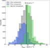 |
Fig. A.2 Histograms of the velocity distributions for single-(grey) and two-component (blue and green) velocity fits to the spectra (see text). The black dashed line shows the velocity boundary, at 35.6 km s−1, used to distribute one velocity component fits in the merged model cube. |
Here Vc,1 and Vc,2 correspond to the velocity center parameter of the first (bluest) and second (reddest) velocity component from the double component model, respectively. This approach ensures the limit reflects a balanced division between the two velocity distributions observed in the histogram in Figure A.2, resulting in a velocity boundary of 35.6 km s−1.
Appendix A.6 Complementary tracers line fitting
For tracers not previously modeled (DCN, H41α, and SiO), we apply a single-Gaussian fit using PySpecKit. The model includes three free parameters: amplitude (Amp), centroid velocity (Vc), and velocity dispersion (σ), with initial guesses derived from the moment maps. Given the simplicity and low computational cost of the model, we do not constrain the parameter ranges. We additionally apply tracer-dependent S/N thresholds through the signal_cut parameter. The S/N is calculated from the peak intensity of each spectrum divided by its RMS noise, estimated from emission-free channels (Table 1).
 |
Fig. A.3 Integrated intensity of the complementary tracers: C18O (J=2−1, upper-left panel; Koley et al. 2025), SiO (J=5−4, upper-right panel; Towner et al. 2024), H41α (bottom left panel; Galván-Madrid et al. 2024), and DCN (J=3−2, bottom right panel; Cunningham et al. 2023). The black contour shows N2H+ integrated intensity at 25 and 100 K km s−1. The scale bar indicates 0.3 pc at the distance of the G012 protocluster. The H41α recombination line and C18O emission are mostly concentrated at the center of G012, where N2H+ is mostly absent and an OB type stars cluster is located (see Fig. 1). In the areas surrounding the main N2H+ filaments, we observe a distribution of lower C18O integrated-intensity emission (~15 K km s−1 ). DCN traces some regions of the main N2H+ structures, and its emission is associated with cores and filaments. Specifically, DCN dominates the top of the R2 filament, central regions of the protocluster, at the edges of R1, and surroundings of the H41α bubbles. |
Appendix B Alternative filament detection using FilFinder
Our current filament selection is based on the visual identification of prominent and kinematically well-separated filamentary structures. More specifically, we are interested in the filamentary structures where the most clear and significatively kinematic patterns are. However, the R1 and R2 selected regions could be part of more extended structures or be conected to other protocluster regions. To addres this, and in order to validate the robustness of our filament selection, we use the FilFinder algortihm to independently identify filamentary structures, which we then compare to our original selection.
FilFinder parameters adopted for the filament detection.
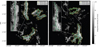 |
Fig. B.1 Results from FilFinder filament detection over the FVC (left panel) and SVC (right panel) integrated-intensity maps. In both panels, the yellow contours represent the final masking area where we apply the algorithm (estimated by SNR and spatial extension considerations), green rigdelines represent the skeletons and branches identifying by FilFinder, black rigdelines shows the filament spine identification in Sect. 4.1 based on the integrated-intensity emission in the R1 and R2 regions. We add a zoom in the R1 and R2 regions to compare the differences between FilFinder (green lines) and our previous (black lines) rigdeline identification. |
Appendix B.1 Method
We use the FilFinder python package (Koch & Rosolowsky 2016) to identify and characterize filamentary structures in 2D emission maps. The analysis is performed on the integrated-intensity maps of each velocity component, since the structures are primarily separated in velocity space (upper panels of Fig. 2). Filament detection is restricted to regions with S/N > 12. The images are first preprocessed using percentile-based flattening to suppress bright compact emission and enhance extended low-contrast structures. Filament masks are then generated through adaptive thresholding, combined with minimum area criteria and optional hole filling to remove small-scale noise features. The minimum filament sizes are selected based on the spatial resolution of the data. Table B.1 summarizes the adopted mask parameters prior to filament identification. All spatial thresholds (see below) are larger than the beam minor axis (2.1" ≈ 0.024 pc), ensuring that the detected structures are spatially resolved filaments.
We adopt a smoothing scale of 5 pixels (0.05 pc; ~2 beam sizes) to reduce pixel-scale noise while preserving resolved filamentary structures. A minimum area threshold of ~0.05 pc2 is used to reject compact or marginally resolved features. The adaptive threshold window is set to ~0.5 pc, matching the characteristic filament scales. We retain only skeletons longer than 0.8 pc to focus on parsec-scale filaments, and prune branches shorter than 0.2 pc to remove minor substructures while preserving the main filamentary morphology. From the final mask, the algorithm computes a medial skeleton representation, reducing each filament to a one-pixel-wide spine (equidistant from the filament edges). This rigdeline estimation differ of our method to estimate the filament spine in Sect. 4.1 where we use the integrated emission in each filament. The resulting skeleton network is analyzed to identify connected components and branches, and is pruned according to length thresholds in order to keep only the main filamentary paths.
Appendix B.2 Variations in physical parameters
In Fig. B.1 we present the results of the FilFinder detection applied to the two velocity component integrated-intensity maps (see upper panels in Fig. 2). The final skeletons identified in the R1 and R2 regions appear more extended than assumed in our baseline definition. Nevertheless, in R1 we recover a ridge line that closely follows the structure adopted in our analysis. In some cases, FilFinder identifies more complex morphologies, particularly in the R2 filament, where most of the elongated structure follows a single main skeleton, but the lower part splits into approximately four possible branches (see right panel in Fig. B.1). Although one could select only the longest path as the main spine of the filament, we consider that it would not be fully reliable to claim that this represents the principal structure. Higher-resolution data will be required to confirm whether these features correspond to dependent or independent substructures near the filament end. For this reason, and to maintain consistency and simplicity in our main kinematic analysis, we restrict our study to the R1 and R2 regions defined at the beginning of this paper (see Fig. 1, right panel), which we consider our main filamentary structures of interest.
To quantify potential variations in our main analysis, we derived key parameters (mass estimation, mass profiles and associated metrics, SFR, and SFF) within the areas identified by FilFinder for the R1 and R2 regions. Within the yellow contours shown in Fig. B.1, which trace the more extended filamentary areas, we derive an H2 mass of 2450 M⊙ for the extended R1 structure and 5000 M⊙ for the extended R2 filament. These values are approximately a factor of two higher than those obtained using our baseline regions alone, emphasizing the significant contribution of these dominant filaments to the total protocluster mass. Overall, about 60% of the protocluster mass is contained within these main filamentary structures.
The cumulative mass profiles of the two extended filaments preserve the approximately linear behavior previously found for R1 and R2. We therefore evaluate how strongly the mass profiles change when considering the extended structures. To align the data, we adopt the FilFinder skeleton output as the ridge-line reference. For R1 we use the single skeleton returned by the algorithm, while for R2 we select the most extended skeleton as the filament ridge line. On average, we find differences of about 30% relative to the metrics derived using only the R1 and R2 regions (see Table 3 for details). The extended filaments show lower M/L values but larger projected radius, which is a direct consequence of the ridge-line alignment. Despite these lower M/L ratios compared to the baseline R1 and R2 regions, the profiles remain significantly higher than those measured in the comparison regions shown in Fig. 6, reinforcing the conclusion that these filaments correspond to highly dense environments and are dominant mass reservoirs in the G012 protocluster.
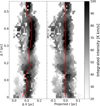 |
Fig. B.2 Example of the R1 filament alignment relative to the integrated-intensity moment map. Left panel: integrated-intensity map of the FVC in the R1 region. The red line represent the ridge line estimated based on the integrated-intensity peak along to the filament. The X and Y axis represent the R1 length and width in units of pc. Right panel: integrated-intensity map aligned respect to the ridge line. The X axis represent the projected radius result of the alignment process. |
In addition, we quantify the number of cores, their classification (prestellar or protostellar), and their masses to estimate the SFR and SFE within the extended areas. In the extended R1 filament, we now identify a protostellar contribution (in contrast to the original R1 selection, which contained only prestellar cores). In total, we detect nine cores in the R1 extension (two proto-stellar and seven prestellar) and 15 cores in the R2 extension (11 protostellar and 4 prestellar). Following the same timescale assumptions described in Sect. 4.3, we estimate the SFR for each core population and for the total. For the extended R1 filament, we derive a prestellar SFR of 6.25 M⊙ Myr−1 and a protostellar SFR of 5.40 M⊙ Myr−1, resulting in a total SFR of 11.65 M⊙ Myr−1, corresponding to an increase of approximately 60% relative to the baseline region. For the extended R2 filament, we estimate a prestellar SFR of 6.3 M⊙ Myr−1 and a protostellar SFR of 47.5 M⊙ Myr−1, yielding a total SFR of 53.9 M⊙ Myr−1, which represents only a 2% difference compared to the baseline region.
For the SFE, the extended R1 region has a total value of 0.0041 (with a prestellar contribution of 0.0030 and a protostellar contribution of 0.0011) that differ in around 60% with the SFE in the original R1 region, while the extended R2 region has a total SFE of 0.0062 (with a prestellar contribution of 0.0015 and a protostellar contribution of 0.0047), here the SFE differs only by 20% respect to our previous estimation in Sect. 4.3. This indicates that the R2 region forms cores with approximately twice the efficiency of the R1 filament. Despite the larger changes in SFR and SFE in the R1 filament, the extended R2 filament maintains a broader diversity in its core population, with a slight tendency toward more evolved cores, and a higher SFR than R1 (SFR in R2 is around a factor of five higher). The main difference compared to the parameters estimated within the smaller baseline regions is that the SFE gap between the two filaments becomes smaller (SFE in R2 is higher by about a factor of 1.5 than in R1).
The kinematic patterns of rotation and collapse discussed in the main analysis for R1 and R2 regions not change when considering the extended filaments. However, we highlight a kinematic transition between the upper and lower parts of the R1 filament. Specifically, the upper part exhibits the rotation signatures discussed in Sect. 4.1, whereas the lower part shows more dispersed velocity patterns and V-shaped structures that we discuss in Sect. 6. This transition may reflect the influence of the core population in that region or the impact of the feedback produced by the H ``II``` bubbles in the region.
Appendix C Data alignment
We apply a filament alignment procedure throughout this work. For example, in Sect. 4.1 the filaments are aligned relative to the peak integrated intensity to estimate average velocity gradients, while in Sect. 4.2 the alignment is based on the column density distribution. Below we describe the procedure for the first case (Fig. B.2), although the same method can be applied to other datasets:
Map rotation: We first rotate the N2H+ maps (e.g., integrated-intensity and velocity centroid) to align the main filaments along the vertical axis (see Fig. 3, upper-left panel).
Ridge-line estimation: Using the N2H+ integrated-intensity map, we estimate the filament ridge line with a custom function that traces the peak intensity along the y-axis, defining the filament spine (red line in Fig. B.2). The procedure is applied independently to the R1 and R2 filaments.
Ridge-line smoothing: We smoothed the ridge line using a one-dimensional uniform filter from scipy.ndimage with a window size of 1 pixel. This reduces sharp fluctuations and produces a smoother representation of the filament path.
Alignment and analysis: The maps are aligned to the smoothed ridge line (Fig. B.2, right panel), transforming the x-axis into projected radius and enabling a more robust analysis of velocity and mass profiles.
Appendix D Technical considerations to estimate relative abundance
Reprojection of the N2H+ column density map can introduce edge artifacts because the regions with sufficient signal-to-noise are highly irregular. To mitigate this effect, we follow the methodology of Sandoval-Garrido et al. (2025) to identify affected pixels: a) We generate a binary mask from the N2H+ column density map, assigning values of 1 to valid pixels and 0 to pixels below the signal-to-noise threshold. b) The mask is reprojected to the H2 pixel scale of Dell'Ova et al. (2024). Pixels with intermediate values between 0 and 1 identify reprojection artifacts, primarily affecting regions within 1–3 pixels of the image boundaries. c) We exclude all pixels with values < 1 in the reprojected mask, producing a reprojection-artifact-free N2H+ column density map.
To analyze the relative abundance distribution, we construct a histogram using the Freedman-Diaconis method (Sandoval-Garrido et al. 2025), obtaining an optimal bin width of 0.377 × 10⁻¹⁰ and 40 bins. We adopt the mode as the representative abundance value, since previous studies showed it is robust against changes in binning (Sandoval-Garrido et al. 2025). For the full sample, the mode is 0.84 × 10⁻¹⁰. To evaluate the impact of stricter τ uncertainty constraints on the abundance estimate, we apply progressively stronger masks:
 (~3% pixels removed)
 (~7% pixels removed)
 (~15% pixels removed)
The mode remains stable between 0.84 × 10⁻¹⁰ and 1.07 × 10⁻¹⁰. To minimize the impact of large τ uncertainties while preserving most of the filamentary structure, we adopt the τ/e(τ) > 2 mask, which removes only ~7% of the pixels.
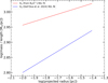 |
Fig. D.1 Mass over length profile of the selected region for the mass validation step. Red line represents the resulting profile considering H2 mass estimated in Sect. 4.3, while blue line shows the final profile considering H2 mass from the column density estimated in Dell'Ova et al. (2024). |
Appendix E Mass validation
To validate the mass selection used for the line-mass profiles (Sect. 4.2), we compare the mass distributions derived from the H2 column density map (Dell'Ova et al. 2024) and the N2H+-based mass estimate from Sect. 3.3. We select a well-detected elongated region within the R2 filament, with a length of 0.4 pc and width of 0.03 pc, and align the filament to compare their cumulative mass distributions. Both distributions follow a similar linear trend, differing only slightly in mass (ΔM ~ 300 M⊙). We therefore derive the M/L profiles following the method described in Sect. 4.2. The resulting profiles show minor differences in slope and the expected offset in normalization (Fig. D.1). We additionally estimate the normalization constants of the apparent volume density (Fq. 5), gravitational potential (Fq. 6), and gravitational acceleration (Fq. 7) using both mass distributions, finding average differences of ~35%.
Given the overall agreement between the two distributions and the improved mass profile obtained for the R1 filament, we adopt the total H2 mass map (Mtot) derived from the N2H+ data for the analysis in Sect. 4.2. Using Mtot, we obtain an approximately linear cumulative mass profile in the R1 filament over a filament length of 0.6 pc (Fig. F.1).
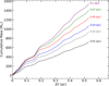 |
Fig. F.1 Fxample of cumulative mass profile in the R1 filament. Color curves highlights cumulative mass measurements at different filament radius. Profiles show a linear trend of the cumulative mass along the filament. |
Appendix F Core velocities
We estimate the velocities of the G012 cores identified in the catalogs described in Sect. 2 using N2H+ and DCN spectral lines. Of the 38 cores previously detected in DCN (Cunningham et al. 2023), 36 are also detected in N2H+ with S/N > 12. We additionally use the 96 continuum cores identified by Armante et al. (2024), 58 of which lack previous velocity measurements. To derive velocities, we fit the DCN and N2H+ emission with a single-Gaussian model (see Appendix A). The major and minor axes of each core (Tables F.1 and F.2) define the region used to extract average spectra and estimate velocity centroids and mean fitted parameters.
From the Armante et al. (2024) catalog, we identify 24 cores detected in both tracers (DCN ⋂ N2H+ sample), 20 detected only in N2H+, 2 detected only in DCN (DCN new sample), and 12 undetected in both tracers. We define VDCN and  as the velocity centroids derived from the DCN and N2H+ fits, respectively. Since DCN traces denser, warmer, and more compact gas, we adopt VDCN when available. To estimate velocities for the N2H+-only sample, we compute the offset
  using 60 cores detected in both tracers: 36 from the previous DCN catalog and 24 from the DCN ⋂ N2H+ sample (similar to the method applied in G353.41 by Álvarez-Gutiérrez et al. 2024).
We find that N2H+ velocities are blueshifted by ~0.16 km s−1 relative to DCN, smaller than the spectral resolutions of both tracers (N2H+: 0.23 km s−1 ; DCN: 0.34 km s−1). Using this correction, we increased the sample of cores with velocity estimates by 48 objects: 24 from the DCN ⋂ N2H+ sample, 20 from the N2H+ sample, and 2 from the DCN new sample.
Cores velocities.
N2H+ velocity differences for DCN core catalog by Cunningham et al. (2023)
All Tables
Line-mass profiles, volume density, gravitational potential, and acceleration distributions.
All Figures
|
Fig. 1 Multiwavelength view and molecular gas distribution of the G012 protocluster. Left panel: Spitzer RGB composite figure of the G012 protocluster at 8 μm (red), 4.5 μm (green), and 3.6 μm (blue). The two cyan contours trace the N2H+ integrated-intensity emission at 25 and 100 K km s−1, respectively. Right panel: N2H+ integrated-intensity map with contours at 25 and 100 K kms−1, corresponding to an S/N > 12, shown in black (same levels as in the left panel). The blue boxes highlight the two main filamentary structures, R1 and R2, with estimated lengths of 0.56 pc for both. We show the average spectra of the two regions in the insets. The black curve represents the data within the black boxes. The red markers represent ionizing regions (crosses), radio sources (plusses), and infrared sources (dots) detected in the region by Haschick & Ho (1983). The green contours show continuum emission from the Atacama Large Millimeter/submillimeter Array Band 6 observations (Ginsburg et al. 2022b). The black ellipse in the bottom right corner represents the beam size of the N2H+ data. |
| In the text | |
|
Fig. 2 N2H+(1−0) integrated intensity (upper panels), velocity centroid (middle panels), and velocity dispersion (bottom panels) of the FVC (left panels) and SVC (right panels). The black contours trace the N2H+ integrated-intensity emission at 25 and 100 K km s−1. The black boxes in all panels display the spatial location of the R1 and R2 filaments. The black ellipse in the bottom right corner represents the beam size of the N2H+ data. |
| In the text | |
|
Fig. 3 Position-position and position-velocity diagrams of the N2H+ observations. Upper left panel: G012 integrated intensity of FVC (blue shades) and SVC (green shades). We display the DCN cores from Cunningham et al. (2023) catalog with black pluses. The Armante et al. (2024) core catalog is divided into four categories: cores only detected with N2H+ (red crosses), cores only detected with DCN data (red circles), cores detected with N2H+ and DCN (red triangles), and cores detected neither in N2H+ nor DCN (black triangles). The symbol sizes are proportional to the estimated core mass. The black ellipse in the bottom right corner represents the beam size of N2H+ data. Upper right panel: PV diagram along the y-axis; the velocity axis is subtracted from the N2H+ systemic VLSR of the protocluster (35.5 km s−1). The black arrow illustrates a slope of 5 pc (km s−1 )−1, which corresponds to a timescale of ~0.2 Myr, that is, the timescales that approximately correspond to some of the extended structures in this PV diagram. At the top of R1, lies a wrapped (or double-helix) type velocity field with spreads of more than ~3 km s−1. On the other hand, R2 appears very compact in velocity along its extent, with small-scale spatial wiggles. Bottom left panel: PV diagram in the perpendicular direction compared to the upper right panel. This shows the emergence, albeit somewhat hidden in the overall velocity field, of an approximately uniform and extended gradient in R1 that is apparent near ΔX ~ 0.60 to 0.75 pc, ΔV ~ −2 to 0 km s−1. In contrast, R2 appears as the compact blob of cores (triangles and x-symbols) on the right-hand-side of the panel, characterized by the absence of an obvious gradient in position and velocity. Bottom right panel: zoomed PV diagrams of the main filaments R1 (left panel) and R2 (right panel), enclosed in the black boxes of the upper left panel. R1 presents a wrapping double-helix signature that is most obvious toward the top of the diagram and which is dominated by the FVC velocities. R2 exhibits comparatively compact velocity variations (ΔVmax~1.5 km s−1) along the filament and contains a high number of massive cores (1–3 M⊙). |
| In the text | |
|
Fig. 4 Left panel: relative abundance map in G012. The black contour highlights the mask of |
| In the text | |
|
Fig. 5 Average velocity gradients perpendicular to R1 (left panel) and R2 (right panel) filaments. In both diagrams, the ΔV and Δr axes have the same range, allowing for a direct comparison of the slopes between the panels. In R1 the red line represents the linear fit weighted by the integrated-intensity points of the velocity gradient (VG). The associated VG timescale (τ) estimate is displayed in the upper left corner. In contrast, R2 lacks a clear velocity gradient structure as in R1 and is instead comparatively compact in its velocity distribution. In addition, we identified two different velocity distributions that spatially correspond to different regions in the R2 filament: 1) the most compact and central structure (compact feature) is related to the densest region of the filament; and 2) the most elongated feature is spatially related to the eastern edge of the R2 filament, characterized by elongated SiO emission. In the diagram, the lower intensity and scattered points represent regions surrounding the filament. |
| In the text | |
|
Fig. 6 Line-mass profile of the R1 and R2 filaments (red lines). The red shaded area represents the uncertainty in the two estimates, derived from the relative abundance uncertainty. This percentage therefore provides a lower limit to the error of 11% in both distributions. We include profiles of the Orion ISF (Stutz & Gould 2016), the ONC (Stutz 2018), the California L1482 region (Álvarez-Gutiérrez et al. 2021), and the G351.77 protocluster (Reyes-Reyes et al. 2024) with black lines. The main filaments of G012 reveal denser line-mass distributions than those found in other star-forming regions. |
| In the text | |
|
Fig. 7 Ratio of the centrifugal (Fc) and gravitational (Fg) forces in the R1 filament (red line), where θ represents the inclination angle of the filament relative to the POS. We assumed cos(θ) = 1, corresponding to a filament aligned with the POS. The red shaded area represents the lower limit error of 11 %, derived from the relative abundance uncertainty. For N2H+, the gravitational force dominates, with a distribution similar to the internal rotation observed in the California L1482-S filament (Álvarez-Gutiérrez et al. 2021). |
| In the text | |
|
Fig. 8 DCN PV diagrams along the R2 filament and toward the central H ``II``` region. The left panel shows a zoom-in of the N2H+ moment 0 map, overlaid with DCN (green) and H41α (yellow) contours. The middle and right panels present DCN PV diagrams extracted from the red and brown boxes shown in the left panel, respectively. The red box highlights the filament extending toward the central H ``II``` bubble in the protocluster, and the brown box traces the R2 filament, including the northern region without N2H+ emission. The red stars indicate the cores detected in DCN (Cunningham et al. 2023). In the middle panel, the dashed black lines mark the center of the H ``II``` bubble (horizontal line) and the systemic velocity estimated from masers (Immer et al. 2014), corresponding to the approximate velocity of the H ``II``` bubble (37 km s−1 ; vertical line). |
| In the text | |
|
Fig. 9 Comparative PV diagrams of California L1482-south (left panel, Álvarez-Gutiérrez et al. 2021), OMC-2 (right panel, González Lobos & Stutz 2019), and the R1 and R2 filaments (center panels). Similar to California, R1 presents a double-helix feature, low presence of cores, and low temperatures (<25 K, see Dell'Ova et al. 2024). Despite this, line-mass profile of both regions (estimated within the range of the red lines on the central panels) shows that R1 is more massive and dense than California L1482-south. Furthermore, R2 shows PV diagram features comparable to the ISF OMC-2 region. Specifically, R2 presents smooth undulations in velocities characterized with uniform velocities. R2 is also characterized by a high presence of cores. |
| In the text | |
|
Fig. A.1 N2H+ two velocity component fitting example: The panels, from top to bottom, display the raw data (grey curve), the first velocity component (blue curve) overlaid on the raw data, the second velocity component (green curve) overlaid on the raw data, the total model (black curve) fitted to the raw data, and the residuals of the model (grey dashed curve). The PySpecKit parameters for the first and second velocity components are shown in each respective panel. |
| In the text | |
|
Fig. A.2 Histograms of the velocity distributions for single-(grey) and two-component (blue and green) velocity fits to the spectra (see text). The black dashed line shows the velocity boundary, at 35.6 km s−1, used to distribute one velocity component fits in the merged model cube. |
| In the text | |
|
Fig. A.3 Integrated intensity of the complementary tracers: C18O (J=2−1, upper-left panel; Koley et al. 2025), SiO (J=5−4, upper-right panel; Towner et al. 2024), H41α (bottom left panel; Galván-Madrid et al. 2024), and DCN (J=3−2, bottom right panel; Cunningham et al. 2023). The black contour shows N2H+ integrated intensity at 25 and 100 K km s−1. The scale bar indicates 0.3 pc at the distance of the G012 protocluster. The H41α recombination line and C18O emission are mostly concentrated at the center of G012, where N2H+ is mostly absent and an OB type stars cluster is located (see Fig. 1). In the areas surrounding the main N2H+ filaments, we observe a distribution of lower C18O integrated-intensity emission (~15 K km s−1 ). DCN traces some regions of the main N2H+ structures, and its emission is associated with cores and filaments. Specifically, DCN dominates the top of the R2 filament, central regions of the protocluster, at the edges of R1, and surroundings of the H41α bubbles. |
| In the text | |
|
Fig. B.1 Results from FilFinder filament detection over the FVC (left panel) and SVC (right panel) integrated-intensity maps. In both panels, the yellow contours represent the final masking area where we apply the algorithm (estimated by SNR and spatial extension considerations), green rigdelines represent the skeletons and branches identifying by FilFinder, black rigdelines shows the filament spine identification in Sect. 4.1 based on the integrated-intensity emission in the R1 and R2 regions. We add a zoom in the R1 and R2 regions to compare the differences between FilFinder (green lines) and our previous (black lines) rigdeline identification. |
| In the text | |
|
Fig. B.2 Example of the R1 filament alignment relative to the integrated-intensity moment map. Left panel: integrated-intensity map of the FVC in the R1 region. The red line represent the ridge line estimated based on the integrated-intensity peak along to the filament. The X and Y axis represent the R1 length and width in units of pc. Right panel: integrated-intensity map aligned respect to the ridge line. The X axis represent the projected radius result of the alignment process. |
| In the text | |
|
Fig. D.1 Mass over length profile of the selected region for the mass validation step. Red line represents the resulting profile considering H2 mass estimated in Sect. 4.3, while blue line shows the final profile considering H2 mass from the column density estimated in Dell'Ova et al. (2024). |
| In the text | |
|
Fig. F.1 Fxample of cumulative mass profile in the R1 filament. Color curves highlights cumulative mass measurements at different filament radius. Profiles show a linear trend of the cumulative mass along the filament. |
| In the text | |
Current usage metrics show cumulative count of Article Views (full-text article views including HTML views, PDF and ePub downloads, according to the available data) and Abstracts Views on Vision4Press platform.
Data correspond to usage on the plateform after 2015. The current usage metrics is available 48-96 hours after online publication and is updated daily on week days.
Initial download of the metrics may take a while.