


| Issue |
A&A
Volume 711, July 2026
Euclid Quick Data Release (Q1)
|
|
|---|---|---|
| Article Number | A13 | |
| Number of page(s) | 28 | |
| Section | Extragalactic astronomy | |
| DOI | https://doi.org/10.1051/0004-6361/202554611 | |
| Published online | 30 June 2026 | |
Euclid Quick Data Release (Q1)
XIII. Exploring galaxy properties with a multi-modal foundation model
1
Instituto de Astrofísica de Canarias (IAC); Departamento de Astrofísica, Universidad de La Laguna (ULL), 38200 La Laguna, Tenerife, Spain
2
Institute of Space Sciences (ICE, CSIC), Campus UAB, Carrer de Can Magrans, s/n, 08193 Barcelona, Spain
3
Instituto de Astrofísica de Canarias, Vía Láctea, 38205 La Laguna, Tenerife, Spain
4
Université PSL, Observatoire de Paris, Sorbonne Université, CNRS, LERMA, 75014 Paris, France
5
Université Paris-Cité, 5 Rue Thomas Mann, 75013 Paris, France
6
School of Physics, Astronomy and Mathematics, University of Hertfordshire, College Lane, Hatfield AL10 9AB, UK
7
UniverseTBD, https://universetbd.org
8
Aspia Space, Falmouth TR10 9TA, UK
9
Instituto de Astrofísica de Andalucía, CSIC, Glorieta de la Astronomía, 18080 Granada, Spain
10
Université Paris-Saclay, Université Paris Cité, CEA, CNRS, AIM, 91191 Gif-sur-Yvette, France
11
Center for Computational Astrophysics, Flatiron Institute, 162 5th Avenue, 10010 New York, NY, USA
12
Center for Cosmology and Particle Physics, Department of Physics, New York University, New York, NY 10003, USA
13
Princeton University, Princeton, NJ 08540, USA
14
Universidad de La Laguna, Departamento de Astrofísica, 38206 La Laguna, Tenerife, Spain
15
Faculdade de Ciências da Universidade do Porto, Rua do Campo de Alegre, 4150-007 Porto, Portugal
16
Instituto de Astrofísica e Ciências do Espaço, Universidade do Porto, CAUP, Rua das Estrelas, PT4150-762 Porto, Portugal
17
Instituto de Física de Cantabria, Edificio Juan Jordá, Avenida de los Castros, 39005 Santander, Spain
18
Leiden Observatory, Leiden University, Einsteinweg 55, 2333 CC Leiden, The Netherlands
19
Kapteyn Astronomical Institute, University of Groningen, PO Box 800, 9700 AV Groningen, The Netherlands
20
INAF-Osservatorio Astronomico di Capodimonte, Via Moiariello 16, 80131 Napoli, Italy
21
Max Planck Institute for Extraterrestrial Physics, Giessenbachstr. 1, 85748 Garching, Germany
22
Institut d’Estudis Espacials de Catalunya (IEEC), Edifici RDIT, Campus UPC, 08860 Castelldefels, Barcelona, Spain
23
School of Physics, HH Wills Physics Laboratory, University of Bristol, Tyndall Avenue, Bristol BS8 1TL, UK
24
Centro de Estudios de Física del Cosmos de Aragón (CEFCA), Plaza San Juan, 1, planta 2, 44001 Teruel, Spain
25
Université Paris-Saclay, CNRS, Institut d’astrophysique spatiale, 91405 Orsay, France
26
ESAC/ESA, Camino Bajo del Castillo, s/n., Urb. Villafranca del Castillo, 28692 Villanueva de la Cañada, Madrid, Spain
27
School of Mathematics and Physics, University of Surrey, Guildford, Surrey GU2 7XH, UK
28
INAF-Osservatorio Astronomico di Brera, Via Brera 28, 20122 Milano, Italy
29
INAF-Osservatorio di Astrofisica e Scienza dello Spazio di Bologna, Via Piero Gobetti 93/3, 40129 Bologna, Italy
30
IFPU, Institute for Fundamental Physics of the Universe, Via Beirut 2, 34151 Trieste, Italy
31
INAF-Osservatorio Astronomico di Trieste, Via G. B. Tiepolo 11, 34143 Trieste, Italy
32
INFN, Sezione di Trieste, Via Valerio 2, 34127 Trieste TS, Italy
33
SISSA, International School for Advanced Studies, Via Bonomea 265, 34136 Trieste TS, Italy
34
Dipartimento di Fisica e Astronomia, Università di Bologna, Via Gobetti 93/2, 40129 Bologna, Italy
35
INFN-Sezione di Bologna, Viale Berti Pichat 6/2, 40127 Bologna, Italy
36
Space Science Data Center, Italian Space Agency, Via del Politecnico snc, 00133 Roma, Italy
37
Dipartimento di Fisica, Università di Genova, Via Dodecaneso 33, 16146 Genova, Italy
38
INFN-Sezione di Genova, Via Dodecaneso 33, 16146 Genova, Italy
39
Department of Physics “E. Pancini”, University Federico II, Via Cinthia 6, 80126 Napoli, Italy
40
Dipartimento di Fisica, Università degli Studi di Torino, Via P. Giuria 1, 10125 Torino, Italy
41
INFN-Sezione di Torino, Via P. Giuria 1, 10125 Torino, Italy
42
INAF-Osservatorio Astrofisico di Torino, Via Osservatorio 20, 10025 Pino Torinese (TO), Italy
43
European Space Agency/ESTEC, Keplerlaan 1, 2201 AZ Noordwijk, The Netherlands
44
Institute Lorentz, Leiden University, Niels Bohrweg 2, 2333 CA Leiden, The Netherlands
45
INAF-IASF Milano, Via Alfonso Corti 12, 20133 Milano, Italy
46
Centro de Investigaciones Energéticas, Medioambientales y Tecnológicas (CIEMAT), Avenida Complutense 40, 28040 Madrid, Spain
47
Port d’Informació Científica, Campus UAB, C. Albareda s/n, 08193 Bellaterra (Barcelona), Spain
48
Institute for Theoretical Particle Physics and Cosmology (TTK), RWTH Aachen University, 52056 Aachen, Germany
49
INAF-Osservatorio Astronomico di Roma, Via Frascati 33, 00078 Monteporzio Catone, Italy
50
INFN section of Naples, Via Cinthia 6, 80126 Napoli, Italy
51
Institute for Astronomy, University of Hawaii, 2680 Woodlawn Drive, Honolulu, HI 96822, USA
52
Dipartimento di Fisica e Astronomia “Augusto Righi” – Alma Mater Studiorum Università di Bologna, Viale Berti Pichat 6/2, 40127 Bologna, Italy
53
Institute for Astronomy, University of Edinburgh, Royal Observatory, Blackford Hill, Edinburgh EH9 3HJ, UK
54
Jodrell Bank Centre for Astrophysics, Department of Physics and Astronomy, University of Manchester, Oxford Road, Manchester M13 9PL, UK
55
European Space Agency/ESRIN, Largo Galileo Galilei 1, 00044 Frascati, Roma, Italy
56
Université Claude Bernard Lyon 1, CNRS/IN2P3, IP2I Lyon, UMR 5822, Villeurbanne F-69100, France
57
Institut de Ciències del Cosmos (ICCUB), Universitat de Barcelona (IEEC-UB), Martí i Franquès 1, 08028 Barcelona, Spain
58
Institució Catalana de Recerca i Estudis Avançats (ICREA), Passeig de Lluís Companys 23, 08010 Barcelona, Spain
59
UCB Lyon 1, CNRS/IN2P3, IUF, IP2I Lyon, 4 rue Enrico Fermi, 69622 Villeurbanne, France
60
Mullard Space Science Laboratory, University College London, Holmbury St Mary, Dorking, Surrey RH5 6NT, UK
61
Departamento de Física, Faculdade de Ciências, Universidade de Lisboa, Edifício C8, Campo Grande, PT1749-016 Lisboa, Portugal
62
Instituto de Astrofísica e Ciências do Espaço, Faculdade de Ciências, Universidade de Lisboa, Campo Grande, 1749-016 Lisboa, Portugal
63
Department of Astronomy, University of Geneva, ch. d’Ecogia 16, 1290 Versoix, Switzerland
64
INAF-Istituto di Astrofisica e Planetologia Spaziali, Via del Fosso del Cavaliere, 100, 00100 Roma, Italy
65
INFN-Padova, Via Marzolo 8, 35131 Padova, Italy
66
Aix-Marseille Université, CNRS/IN2P3, CPPM, Marseille, France
67
INFN-Bologna, Via Irnerio 46, 40126 Bologna, Italy
68
Universitäts-Sternwarte München, Fakultät für Physik, Ludwig-Maximilians-Universität München, Scheinerstrasse 1, 81679 München, Germany
69
INAF-Osservatorio Astronomico di Padova, Via dell’Osservatorio 5, 35122 Padova, Italy
70
NRC Herzberg, 5071 West Saanich Rd, Victoria, BC V9E 2E7, Canada
71
Institute of Theoretical Astrophysics, University of Oslo, P.O. Box 1029 Blindern, 0315 Oslo, Norway
72
Jet Propulsion Laboratory, California Institute of Technology, 4800 Oak Grove Drive, Pasadena, CA 91109, USA
73
Department of Physics, Lancaster University, Lancaster LA1 4YB, UK
74
Felix Hormuth Engineering, Goethestr. 17, 69181 Leimen, Germany
75
Technical University of Denmark, Elektrovej 327, 2800 Kgs. Lyngby, Denmark
76
Cosmic Dawn Center (DAWN), Denmark
77
Max-Planck-Institut für Astronomie, Königstuhl 17, 69117 Heidelberg, Germany
78
NASA Goddard Space Flight Center, Greenbelt, MD 20771, USA
79
Department of Physics and Helsinki Institute of Physics, Gustaf Hällströmin katu 2, 00014 University of Helsinki, Finland
80
Université de Genève, Département de Physique Théorique and Centre for Astroparticle Physics, 24 quai Ernest-Ansermet, CH-1211 Genève 4, Switzerland
81
Department of Physics, P.O. Box 64, 00014 University of Helsinki, Finland
82
Helsinki Institute of Physics, Gustaf Hällströmin katu 2 University of Helsinki, Helsinki, Finland
83
Centre de Calcul de l’IN2P3/CNRS, 21 avenue Pierre de Coubertin 69627 Villeurbanne Cedex, France
84
Laboratoire d’etude de l’Univers et des phenomenes eXtremes, Observatoire de Paris, Université PSL, Sorbonne Université, CNRS, 92190 Meudon, France
85
Aix-Marseille Université, CNRS, CNES, LAM, Marseille, France
86
SKA Observatory, Jodrell Bank, Lower Withington, Macclesfield, Cheshire SK11 9FT, UK
87
Dipartimento di Fisica “Aldo Pontremoli”, Università degli Studi di Milano, Via Celoria 16, 20133 Milano, Italy
88
INFN-Sezione di Milano, Via Celoria 16, 20133 Milano, Italy
89
University of Applied Sciences and Arts of Northwestern Switzerland, School of Computer Science, 5210 Windisch, Switzerland
90
Universität Bonn, Argelander-Institut für Astronomie, Auf dem Hügel 71, 53121 Bonn, Germany
91
INFN-Sezione di Roma, Piazzale Aldo Moro, 2 – c/o Dipartimento di Fisica, Edificio G. Marconi, 00185 Roma, Italy
92
Dipartimento di Fisica e Astronomia “Augusto Righi” – Alma Mater Studiorum Università di Bologna, Via Piero Gobetti 93/2, 40129 Bologna, Italy
93
Department of Physics, Institute for Computational Cosmology, Durham University, South Road, Durham DH1 3LE, UK
94
Université Côte d’Azur, Observatoire de la Côte d’Azur, CNRS, Laboratoire Lagrange, Bd de l’Observatoire, CS 34229, 06304 Nice cedex 4, France
95
Institut d’Astrophysique de Paris, UMR 7095, CNRS, and Sorbonne Université, 98 bis boulevard Arago, 75014 Paris, France
96
Université Paris Cité, CNRS, Astroparticule et Cosmologie, 75013 Paris, France
97
CNRS-UCB International Research Laboratory, Centre Pierre Binétruy, IRL2007, CPB-IN2P3, Berkeley, USA
98
University of Applied Sciences and Arts of Northwestern Switzerland, School of Engineering, 5210 Windisch, Switzerland
99
Institut d’Astrophysique de Paris, 98bis Boulevard Arago, 75014 Paris, France
100
Institute of Physics, Laboratory of Astrophysics, Ecole Polytechnique Fédérale de Lausanne (EPFL), Observatoire de Sauverny, 1290 Versoix, Switzerland
101
Aurora Technology for European Space Agency (ESA), Camino bajo del Castillo, s/n, Urbanizacion Villafranca del Castillo, Villanueva de la Cañada, 28692 Madrid, Spain
102
Institut de Física d’Altes Energies (IFAE), The Barcelona Institute of Science and Technology, Campus UAB, 08193 Bellaterra (Barcelona), Spain
103
School of Mathematics, Statistics and Physics, Newcastle University, Herschel Building, Newcastle-upon-Tyne, NE1 7RU, UK
104
DARK, Niels Bohr Institute, University of Copenhagen, Jagtvej 155, 2200 Copenhagen, Denmark
105
Waterloo Centre for Astrophysics, University of Waterloo, Waterloo, Ontario N2L 3G1, Canada
106
Department of Physics and Astronomy, University of Waterloo, Waterloo, Ontario N2L 3G1, Canada
107
Perimeter Institute for Theoretical Physics, Waterloo, Ontario N2L 2Y5, Canada
108
Centre National d’Etudes Spatiales – Centre spatial de Toulouse, 18 avenue Edouard Belin, 31401 Toulouse Cedex 9, France
109
Institute of Space Science, Str. Atomistilor, nr. 409Măgurele, Ilfov 077125, Romania
110
Dipartimento di Fisica e Astronomia “G. Galilei”, Università di Padova, Via Marzolo 8, 35131 Padova, Italy
111
Institut für Theoretische Physik, University of Heidelberg, Philosophenweg 16, 69120 Heidelberg, Germany
112
Institut de Recherche en Astrophysique et Planétologie (IRAP), Université de Toulouse, CNRS, UPS, CNES, 14 Av. Edouard Belin, 31400 Toulouse, France
113
Université St Joseph; Faculty of Sciences, Beirut, Lebanon
114
Departamento de Física, FCFM, Universidad de Chile, Blanco Encalada 2008, Santiago, Chile
115
Universität Innsbruck, Institut für Astro- und Teilchenphysik, Technikerstr. 25/8, 6020 Innsbruck, Austria
116
Satlantis, University Science Park, Sede Bld 48940, Leioa-Bilbao, Spain
117
Instituto de Astrofísica e Ciências do Espaço, Faculdade de Ciências, Universidade de Lisboa, Tapada da Ajuda, 1349-018 Lisboa, Portugal
118
Cosmic Dawn Center (DAWN)
119
Niels Bohr Institute, University of Copenhagen, Jagtvej 128, 2200 Copenhagen, Denmark
120
Universidad Politécnica de Cartagena, Departamento de Electrónica y Tecnología de Computadoras, Plaza del Hospital 1, 30202 Cartagena, Spain
121
Infrared Processing and Analysis Center, California Institute of Technology, Pasadena, CA 91125, USA
122
Dipartimento di Fisica e Scienze della Terra, Università degli Studi di Ferrara, Via Giuseppe Saragat 1, 44122 Ferrara, Italy
123
Istituto Nazionale di Fisica Nucleare, Sezione di Ferrara, Via Giuseppe Saragat 1, 44122 Ferrara, Italy
124
INAF, Istituto di Radioastronomia, Via Piero Gobetti 101, 40129 Bologna, Italy
125
Department of Physics, Oxford University, Keble Road, Oxford OX1 3RH, UK
126
INAF – Osservatorio Astronomico di Brera, Via Emilio Bianchi 46, 23807 Merate, Italy
127
INAF-Osservatorio Astronomico di Brera, Via Brera 28, 20122 Milano, Italy, and INFN-Sezione di Genova, Via Dodecaneso 33, 16146 Genova, Italy
128
ICL, Junia, Université Catholique de Lille, LITL, 59000 Lille, France
129
ICSC – Centro Nazionale di Ricerca in High Performance Computing, Big Data e Quantum Computing, Via Magnanelli 2, Bologna, Italy
130
Instituto de Física Teórica UAM-CSIC, Campus de Cantoblanco, 28049 Madrid, Spain
131
CERCA/ISO, Department of Physics, Case Western Reserve University, 10900 Euclid Avenue, Cleveland, OH 44106, USA
132
Technical University of Munich, TUM School of Natural Sciences, Physics Department, James-Franck-Str. 1, 85748 Garching, Germany
133
Max-Planck-Institut für Astrophysik, Karl-Schwarzschild-Str. 1, 85748 Garching, Germany
134
Laboratoire Univers et Théorie, Observatoire de Paris, Université PSL, Université Paris Cité, CNRS, 92190 Meudon, France
135
Departamento de Física Fundamental. Universidad de Salamanca, Plaza de la Merced s/n, 37008 Salamanca, Spain
136
Université de Strasbourg, CNRS, Observatoire astronomique de Strasbourg, UMR 7550, 67000 Strasbourg, France
137
Center for Data-Driven Discovery, Kavli IPMU (WPI), UTIAS, The University of Tokyo, Kashiwa, Chiba 277-8583, Japan
138
California Institute of Technology, 1200 E California Blvd, Pasadena, CA 91125, USA
139
Department of Physics & Astronomy, University of California Irvine, Irvine CA 92697, USA
140
Department of Mathematics and Physics E. De Giorgi, University of Salento, Via per Arnesano, CP-I93, 73100 Lecce, Italy
141
INFN, Sezione di Lecce, Via per Arnesano, CP-193, 73100 Lecce, Italy
142
INAF-Sezione di Lecce, c/o Dipartimento Matematica e Fisica, Via per Arnesano, 73100 Lecce, Italy
143
Departamento Física Aplicada, Universidad Politécnica de Cartagena, Campus Muralla del Mar, 30202 Cartagena, Murcia, Spain
144
CEA Saclay, DFR/IRFU, Service d’Astrophysique, Bat. 709, 91191 Gif-sur-Yvette, France
145
Institute of Cosmology and Gravitation, University of Portsmouth, Portsmouth PO1 3FX, UK
146
Department of Computer Science, Aalto University, PO Box 15400 Espoo FI-00 076, Finland
147
Instituto de Astrofísica de Canarias, c/ Via Lactea s/n, La Laguna 38200, Spain. Departamento de Astrofísica de la Universidad de La Laguna, Avda. Francisco Sanchez, La Laguna, 38200, Spain
148
Caltech/IPAC, 1200 E. California Blvd., Pasadena, CA 91125, USA
149
Ruhr University Bochum, Faculty of Physics and Astronomy, Astronomical Institute (AIRUB), German Centre for Cosmological Lensing (GCCL), 44780 Bochum, Germany
150
Department of Physics and Astronomy, Vesilinnantie 5, 20014 University of Turku, Finland
151
Serco for European Space Agency (ESA), Camino bajo del Castillo, s/n, Urbanizacion Villafranca del Castillo, Villanueva de la Cañada, 28692 Madrid, Spain
152
ARC Centre of Excellence for Dark Matter Particle Physics, Melbourne, Australia
153
Centre for Astrophysics & Supercomputing, Swinburne University of Technology, Hawthorn, Victoria 3122, Australia
154
Department of Physics and Astronomy, University of the Western Cape, Bellville, Cape Town, 7535, South Africa
155
DAMTP, Centre for Mathematical Sciences, Wilberforce Road, Cambridge CB3 0WA, UK
156
Kavli Institute for Cosmology Cambridge, Madingley Road, Cambridge CB3 0HA, UK
157
Department of Astrophysics, University of Zurich, Winterthurerstrasse 190, 8057 Zurich, Switzerland
158
Department of Physics, Centre for Extragalactic Astronomy, Durham University, South Road, Durham DH1 3LE, UK
159
IRFU, CEA, Université Paris-Saclay, 91191 Gif-sur-Yvette Cedex, France
160
Oskar Klein Centre for Cosmoparticle Physics, Department of Physics, Stockholm University, Stockholm SE-106 91, Sweden
161
Astrophysics Group, Blackett Laboratory, Imperial College London, London SW7 2AZ, UK
162
Univ. Grenoble Alpes, CNRS, Grenoble INP, LPSC-IN2P3, 53, Avenue des Martyrs, 38000 Grenoble, France
163
INAF-Osservatorio Astrofisico di Arcetri, Largo E. Fermi 5, 50125 Firenze, Italy
164
Dipartimento di Fisica, Sapienza Università di Roma, Piazzale Aldo Moro 2, 00185 Roma, Italy
165
Centro de Astrofísica da Universidade do Porto, Rua das Estrelas, 4150-762 Porto, Portugal
166
HE Space for European Space Agency (ESA), Camino bajo del Castillo, s/n, Urbanizacion Villafranca del Castillo, Villanueva de la Cañada, 28692 Madrid, Spain
167
Dipartimento di Fisica – Sezione di Astronomia, Università di Trieste, Via Tiepolo 11, 34131 Trieste, Italy
168
Department of Astrophysical Sciences, Peyton Hall, Princeton University, Princeton, NJ 08544, USA
169
Theoretical astrophysics, Department of Physics and Astronomy, Uppsala University, Box 516, 751 37 Uppsala, Sweden
170
Mathematical Institute, University of Leiden, Einsteinweg 55, 2333 CA Leiden, The Netherlands
171
Institute of Astronomy, University of Cambridge, Madingley Road, Cambridge CB3 0HA, UK
172
Space physics and astronomy research unit, University of Oulu, Pentti Kaiteran katu 1, FI-90014 Oulu, Finland
173
Univ. Lille, CNRS, Centrale Lille, UMR 9189 CRIStAL, 59000 Lille, France
★ Corresponding author: This email address is being protected from spambots. You need JavaScript enabled to view it.
Received:
18
March
2025
Accepted:
23
May
2025
Abstract
Modern astronomical surveys, such as the Euclid mission, produce high-dimensional, multi-modal datasets that include imaging and spectroscopic information for millions of galaxies. These data serve as an ideal benchmark for large, pre-trained multi-modal models, which can leverage vast amounts of unlabelled data. In this work, we present the first exploration of Euclid data with AstroPT, an autoregressive multi-modal foundation model trained on approximately 300000 optical and infrared Euclid images and spectral energy distributions (SEDs) from the first Euclid Quick Data Release. We compare self-supervised pre-training with baseline fully supervised training across several tasks: galaxy morphology classification; redshift estimation; similarity searches; and outlier detection. Our results show that: (a) AstroPT embeddings are highly informative, correlating with morphology and effectively isolating outliers; (b) including infrared data helps to isolate stars, but degrades the identification of edge-on galaxies, which are better captured by optical images; (c) simple fine-tuning of these embeddings for photometric redshift and stellar mass estimation outperforms a fully supervised approach, even when using only 1% of the training labels; and (d) incorporating SED data into AstroPT via a straightforward multi-modal token-chaining method improves photo-z predictions, and allow us to identify potentially more interesting anomalies (such as ringed or interacting galaxies) compared to a model pre-trained solely on imaging data.
Key words: methods: data analysis / galaxies: general
© The Authors 2026
 Open Access article, published by EDP Sciences, under the terms of the Creative Commons Attribution License (https://creativecommons.org/licenses/by/4.0), which permits unrestricted use, distribution, and reproduction in any medium, provided the original work is properly cited.
This article is published in open access under the Subscribe to Open model. This email address is being protected from spambots. You need JavaScript enabled to view it. to support open access publication.
1. Introduction
Astronomy’s abundance of data requires appropriately scalable, automated frameworks to be mined effectively. This demand has already driven the adoption of advanced machine-learning and deep-learning techniques for a variety of purposes (see for example Domínguez Sánchez et al. 2018; Cheng et al. 2020, 2021; Vega-Ferrero et al. 2021; Walmsley et al. 2022a, 2023; Huertas-Company et al. 2024, or see Huertas-Company & Lanusse 2023; Smith & Geach 2023 for general reviews). However, in most prior work a small subset of labelled examples have been used to train supervised models. This means that only a small fraction of available data is used, and that the trained models are very sensitive to ‘domain drift’ (Domínguez Sánchez et al. 2019), thus limiting their full deployment for scientific analysis (Huertas-Company & Lanusse 2023).
Recent works have demonstrated the transformative impact of models pre-trained on large amounts of unlabelled data (that is, ‘foundation models’), which can then be fine-tuned to perform a variety of tasks. This is particularly evident for language processing, in which the best-performing ‘frontier’ models now contain many billions of parameters and require ‘web-scale’ data of the order of terabytes to petabytes to be sufficiently pre-trained (e.g. Grattafiori et al. 2024). Furthermore, the recent rediscovery of neural scaling laws – empirical relationships that demonstrate how model performance improves predictably with increases in model size, dataset size, or computational resources – has led to great growth in the size of deep-learning models (Cortes et al. 1993; Kaplan et al. 2020; Henighan et al. 2020).
Astronomical datasets are also growing rapidly in size and complexity, creating the need for models that can scale with dataset size and perform multiple tasks effectively (Smith et al. 2024; Pan et al. 2024; Walmsley et al. 2024; Merz et al. 2025; The Multimodal Universe Collaboration 2024). The advent of the next generation of large-scale sky surveys such as Euclid (Laureijs et al. 2011), the Dark Energy Spectroscopic Instrument Legacy Survey (DESI; DESI Collaboration 2022, 2024a), and the Vera C. Rubin Legacy Surveys of Space and Time (LSST; Ivezić et al. 2019) opens new opportunities for developing a new generation of astronomical foundation models. These datasets offer multi-wavelength imaging and spectroscopy of millions of galaxies with relatively little labelled data, and thus provide an ideal sandbox for developing the next generation of machine-learning models. Euclid’s mission is especially valuable for its combination of high-resolution imaging with spectroscopy over a wide field of view, which creates a unique opportunity for advancing the next generation of large-scale machine-learning models. This synergy between cutting-edge surveys and artificial intelligence-driven methods will be instrumental in accelerating the adoption of machine learning in astrophysics (Euclid Collaboration: Humphrey et al. 2023; Euclid Collaboration: Leuzzi et al. 2024; Euclid Collaboration: Aussel et al. 2024; Euclid Collaboration: Enia et al. 2024; Euclid Collaboration: Mellier et al. 2025).
Several works have started exploring large pre-trained models in astronomy (e.g. Vega-Ferrero et al. 2024). Hayat et al. (2021) and Sarmiento et al. (2021) first demonstrated the quality of the embedding spaces on Sloan Digital Sky Survey (SDSS; Gunn et al. 1998, 2006) and Mapping Nearby Galaxies at APO (MaNGA; Bundy et al. 2015) data using contrastive learning, a self-supervised technique whereby a model is trained to bring similar samples closer in an embedding space while pushing dissimilar ones apart (Chen et al. 2020; Radford et al. 2021). Smith et al. (2024) showed that autoregressive galaxy imaging models follow similar scaling laws to the ones reported for text. Complementing these imaging methods, AstroCLIP (Parker et al. 2024) pioneered a multi-modal strategy by aligning spectra and imaging via contrastive learning. Following a similar approach, the PAPERCLIP framework (Mishra-Sharma et al. 2024) explores the intersection of astronomical imaging and natural language by fine-tuning a contrastive language–image pre-training (CLIP; Radford et al. 2021) CLIP model to align observations (e.g. galaxy images) and textual descriptions. This allows users to search for images based on descriptive language, and vice versa. Zhang et al. (2024) and Rizhko & Bloom (2025) present the first attempts to incorporate time-series data with CLIP, constructing an astronomical multi-modal dataset from time-series photometry data, spectra, and astrophysical metadata. These advancements illustrate the expanding frontier of multi-modal approaches, which combine data modalities to provide a more comprehensive understanding of astronomical phenomena. As just one example of a downstream use-case, researchers can use these models to gain insights into both the structural properties and the dynamical evolution of galaxies, reaching a state-of-the-art performance on classification and redshift estimation without any explicit optimisations towards these tasks.
Following these developments, in this work we pre-train and use a multi-modal autoregressive foundation model (AstroPT) to explore the optical and infrared imaging components and the spectral energy distributions (SEDs) of Euclid Q1 galaxies (Euclid Quick Release Q1 2025). Multi-modal models are capable of integrating and learning from different types of data (such as images, spectra, and text) simultaneously, while autoregressive models predict data sequentially by learning dependencies across inputs, such as pixel sequences in images or wavelength features in spectra or SEDs. Furthermore, autoregressive models can operate on the union of available observations without being restricted solely to cross-matched datasets, which typically represent only a small fraction of the available data. These properties make models like AstroPT wellsuited to analysing the diverse, high-dimensional data produced by modern surveys. In Fig. 1 we illustrate the rapid growth of foundation models in astronomy, demonstrating an increasing trend in model size as astronomical datasets expand. This trend is motivated by model scaling laws – empirical observations that model performance improves predictably with increasing data, compute, or parameter count, provided the other two are sufficient (Kaplan et al. 2020; Hoffmann et al. 2022). While recent work has started to explore potential environmental and economic limitations to these laws (e.g. Muennighoff et al. 2023; Diaz & Madaio 2023; Sengupta et al. 2025), they remain a useful guide for forecasting model capabilities, and thus continue to drive the state of the art in language modelling. We define the number of tokens as subword units for text (GPT), image pairs for contrastive models, or image patches for the AstroPT model. With each new Euclid data release – assuming that galaxy scaling laws hold in the same way as was previously found in textual models – models are projected to scale closer to the size of GPT-2 and GPT-3, large-scale transformer-based language models developed by OpenAI, representing significant advancements in natural language processing (Brown et al. 2020). Additionally, incorporating spectral data into multi-modal models significantly enhances their complexity, potentially requiring a further increase in model size.
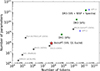 |
Fig. 1. Scaling laws for foundation models in astronomy compared to the GPT series. The number of tokens is defined as subword units in text (GPT models); pairs of augmented images (contrastive learning models); or a number of patches (AstroPT model). The projected scaling of future models incorporating Euclid data in upcoming data releases are marked with green stars. Our current model, trained on Q1 Euclid data, is represented by a red star. The models from the literature are referenced as follows: AH21 (Hayat et al. 2021); S21 (Sarmiento et al. 2021), GS21 (Stein et al. 2021); GMS24 (Martínez-Solaeche et al. 2024); P24 (Parker et al. 2024); and MS24 (Smith et al. 2024). |
We evaluate the performance of an AstroPT model on a variety of downstream tasks – specific, practical applications of a pre-trained model – such as galaxy morphology classification, redshift prediction, or stellar mass estimations. By comparing these results to those achieved by a baseline fully supervised model, we assess the advantages of pre-training and multi-modal learning for astronomical data analysis. Unsupervised and self-supervised learning methods are particularly appealing for downstream tasks because they can generate semantically meaningful representations without requiring extensive labelled datasets. Such methods were successfully applied in astronomy for galaxy morphology studies (e.g. Hocking et al. 2018; Slijepcevic et al. 2024), estimations of photometric redshift (photo-z; e.g. Merz et al. 2025; Pattnaik et al. 2025), and physical properties (e.g. Euclid Collaboration: Bisigello et al. 2023; Chu et al. 2024; Euclid Collaboration: Enia et al. 2024; Gai et al. 2024), as well as for anomaly detection (see Fotopoulou 2024, for a review), and similarity searches (e.g. Stein et al. 2021; Walmsley et al. 2022b; Parker et al. 2024). Recent advancements in self-supervised learning have significantly closed the performance gap between unsupervised and supervised learning (e.g. Cheng et al. 2020; Mohale & Lochner 2024), with self-supervised models now achieving comparable accuracy on downstream tasks such as classification and regression.
This paper is structured as follows. In Sect. 2, we introduce the Euclid mission and the Q1 sample selection. The AstroPT framework is presented in Sect. 3, together with other approaches to predict galaxy properties. In Sect. 4 we discuss the performance of AstroPT on Euclid imaging data, in comparison to other methods. Section 5 summarises the main results. In Appendix A the hyperparameters of the model are given, Appendix B presents the embeddings for VIS, and NISP imaging. The star–galaxy separation is discussed in Appendix C, and physical properties in Appendix D. Finally, the accuracy of morphological classification, and predictions of stellar masses and photo-z is detailed in Appendix E.
2. Data
The Euclid mission, launched in 2023, is a mission of the European Space Agency (ESA) that is dedicated to investigating the nature of dark energy, and dark matter by measuring the accelerated expansion of the Universe. Euclid primarily focuses on gathering high-resolution imaging and spectroscopic data of around 109 galaxies out to z ≈ 3, and millions of galaxies out to z ≈ 6 over 14 000 deg2 (Euclid Collaboration: Mellier et al. 2025). Euclid provides broadband optical imaging through the visible imaging channel (VIS; Euclid Collaboration: McCracken et al. 2026), and multi-band near-infrared spectroscopy and imaging with the near-infrared spectrometer and photometer (NISP; Euclid Collaboration: Jahnke et al. 2025). The VIS instrument captures optical data in the visible range corresponding to r, i, and z filters (IE covers λ = 0.53–0.92 μm; Euclid Collaboration: Cropper et al. 2025), with a spatial resolution of approximately 0 18 (Euclid Collaboration: Cropper et al. 2025). This high-resolution imaging provides an excellent foundation for morphological studies, allowing for the extraction of detailed structural properties of galaxies. The NISP captures infrared data (YE, JE, and HE cover λ = 0.95–2.02 μm; Euclid Collaboration: Schirmer et al. 2022) and is designed for photometric redshift (photo-z) determination and galaxy clustering measurements, which complement the VIS data by providing additional depth and accuracy for cosmic surveys.
2.1. Q1 sample
As part of the Euclid mission, Q1 represents the first major public data release. Q1 provides a snapshot of early observations taken during the initial phase of the mission, covering ∼29.7 million sources over 63 deg2 of the Euclid Deep Fields (EDFs). These fields are the Euclid Deep Field North (EDF-N), the Euclid Deep Field South (EDF-S), and Euclid Deep Field Fornax (EDF-F). The Q1 release includes raw and processed images (calibrated VIS, NISP frames, and background-subtracted mosaics, and segmentation maps), along with the MER photometric catalogue (Euclid Collaboration: Romelli et al. 2026). A detailed description of the Q1 data release is presented in Euclid Collaboration: Aussel et al. (2026), Euclid Collaboration: McCracken et al. (2026), Euclid Collaboration: Polenta et al. (2026), and Euclid Collaboration: Romelli et al. (2026).
The MER catalogue includes multi-wavelength photometry, combining data from Euclid VIS and NISP photometry with external photometric surveys spanning the ultraviolet to the near-infrared wavelengths. In particular, the catalogue includes fluxes in the IE, HE, JE, and YEEuclid bands, complemented by optical bands (u, g, r, i, and z) from the Dark Energy Survey (Dark Energy Survey Collaboration 2016), and the ultraviolet near-infrared optical northern survey (UNIONS; Gwyn et al. in prep.). UNIONS imaging includes CFHT u, r, HSC g, z, and Pan-STARRS i, z, and is an independent collaboration aimed at enhancing the scientific yield of large and deep surveys of the northern sky. To ensure robust cross-ground-based survey comparisons, the photometry is measured using A-PHOT (Merlin et al. 2019), employing fixed circular apertures with diameters of two full widths at half maximum (FWHMs) of the worstseeing band (typically around 2″), computed individually for each source based on PSF-matched images. The bands used to construct SEDs (i.e. the collection of photometric measurements), and their corresponding fields are listed in Table 1.
Photometric bands, instruments, observed depths, and fields included in the Euclid photometric catalogue used to build the SEDs of Q1 sources.
This dataset is further complemented by a {star, galaxy, quasar (QSO)} trinary classification, the photo-z, and galaxy physical properties estimated with the k-nearest-neighbour algorithm (NNPZ; Tanaka et al. 2018; Euclid Collaboration: Enia et al. 2024, 2026; Euclid Collaboration: Tucci et al. 2026), among others. While these estimates are useful for certain downstream tasks (see Sect. 4.2), spectroscopic redshifts (DESI Collaboration 2024b) and stellar masses (Siudek et al. 2024) from DESI are used for validation to ensure reliability. The DESI sample constitutes only a small fraction of the entire Q1 dataset, and does not cover the full panoply of Euclid Q1 galaxies (see Fig. 2).
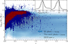 |
Fig. 2. Stellar mass-redshift relation for the Q1 sample (in cyan), the sample used in this work (in navy blue), and our sample with DESI spectroscopic information (in red). The inset plots show the residuals of redshift and stellar mass differences between the Euclid pipeline and DESI, respectively. |
2.2. Parent sample
In this work, we have selected sources with a segmentation area greater than 800 pixels in the VIS data, which corresponds to galaxies that are sufficiently large to have accurate morphological classifications (Euclid Collaboration: Walmsley et al. 2026a). The Euclid survey operates with a pixel scale of approximately 0 1 per pixel, corresponding to a physical resolution of approximately 0.5 kpc at z ≈ 0.5. This criterion ensures that the sample includes only well-resolved objects, allowing for accurate morphological characterisation. We additionally restricted our sample to galaxies with HE < 22.5. This magnitude limit ensures the inclusion of objects that are bright enough to be detectable in the near-infrared bands, which is crucial for obtaining their spectra. Figure 3 shows the distribution of Euclid magnitudes for sources in our sample, broken down by the IE, YE, JE, and HE bands. For the selected sample, the images are complemented with the SEDs of sources covering the optical through to infrared fluxes. An example SED constructed from Euclid and auxiliary survey data is shown in Figure 4. This work solely builds on the imaging and photometric data, while we leave the addition of the spectra for future work.
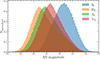 |
Fig. 3. Distribution of Euclid photometry for the sample used in this paper. |
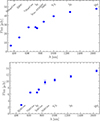 |
Fig. 4. Representative SEDs of galaxies from the Q1 EDF-N (top) and EDF-S fields (bottom). The SED includes multi-wavelength photometric data spanning the ultraviolet to the near-infrared listed in Table 1. |
Our final set comprises approximately 330 000 galaxies spread across the Q1 fields, shown in blue in Fig. 2. We split our galaxy dataset using an 80/10/10 training-test-validation split. This selection introduces constraints in both redshift and stellar mass, which may influence the representation of our data and the performance of downstream tasks. In particular, our sample is mostly limited to z ≲ 1 and log10(M*/M⊙) ≳ 7. These cuts ensure higher-quality images for our analysis but could introduce biases, particularly in studies of low-mass and high-redshift galaxies. The spectroscopic subset from DESI further refines the selection, potentially impacting our ability to characterise the most massive systems with precise redshift information.
3. Methodology
In this section, we outline the machine learning methodologies employed to analyse the galaxy dataset, starting with AstroPT in Sect. 3.1. In Sect. 3.2 we introduce three separate models used to evaluate the performance of different techniques in downstream tasks (Sect. 4.2).
3.1. AstroPT
AstroPT1 is an autoregressive transformer designed to extract scientifically useful embeddings from high-resolution galaxy images. A visualisation of the AstroPT architecture is shown in the right panel in Fig. 5. Due to space constraints, we do not go into detail about the transformer architecture in this paper. We instead recommend Sect. 4(d) of Smith & Geach (2023) for an astronomy-friendly introduction of the transformer model, and Sects. 7 and 9 of the same publication for a further discussion of the ideas behind AstroPT and other foundation models.
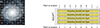 |
Fig. 5. AstroPT’s training objective is predicting the next patch in a sequence of galaxy image (and other modalities’) patches. On the left we show the order of galaxy patches used in this work, and on the right we show how each patch is processed by AstroPT. |
AstroPT is initially trained to predict the next image patch in a sequence of image patches. This training process incentivises the model to learn a compact representation of the data, which captures the essential patterns and relationships inherent in the astronomical observations it is pre-trained on. Our dataset consists of 224 × 224 pixel FITS cut-outs in the VIS and NISP bands fixed to the same angular size from mosaics, i.e. MER background-subtracted calibrated frames. The cut-out size is an arbitrary choice, corresponding to a commonly used input size for deep-learning models due to their compatibility with standard convolutional neural network architectures and AstroCLIP (Parker et al. 2024). The fixed size allows for efficient training on GPUs while maintaining a balance between spatial resolution and computational cost. However, this choice has implications for the representation of galaxy morphology: (i) smaller galaxies may be dominated by background noise or multiple objects might be in the frame; and (ii) larger galaxies might not fit entirely within the cut-out, leading to truncation of their outer regions. These effects introduce potential biases into the embeddings, as their descriptive power may depend on the relative size of the galaxy within the cut-out. A potential way to mitigate these biases would be to adopt a variable cut-out size based on the galaxy’s angular size (e.g. Petrosian radius or half-light radius), enabling better coverage of large galaxies while minimising background contamination in small ones. For images, the training process involves optimising a Huber loss (Huber 1964) objective, with the model attempting to predict the next 16 × 16 pixel patch in a sequence of galaxy image patches (as illustrated in the left panel of Fig. 5). In this study, we use the same model architecture as the 90 million parameter model described in Smith et al. (2024). To ensure consistency across inputs, each image patch is normalised by taking its zscore, defined as
 (1)
(1)
where x is the pixel value, μ is the mean, and σ is the standard deviation of the pixel values across the patch. This normalisation centres the data around zero and scales it to have unit variance, improving stability during pre-training (e.g. El-Nouby et al. 2024). However, we acknowledge that global normalisation may have an impact on information, like a contrast reduction in faint structures, particularly in the outskirts of galaxies. The verification of alternative normalisation strategies, such as local normalisation or ‘min-max’ scaling, is left to future work. To incorporate SEDs, we used a simple token-chaining mechanism. This process involves concatenating the SED data as a token sequence to be fed in after the imaging tokens allowing the model to process both modalities (imaging, and SED information) simultaneously. The SEDs are divided into patches of a length of one, and the SEDs are normalised using the z-score over the entire SED sequence. While the zscore normalisation preserves the relative shape of SEDs, it could, in principle, reduce the distinctiveness of extreme SEDs (e.g. very blue or very red galaxies). Testing alternative approaches, such as converting fluxes to magnitudes before normalisation, is left for future work. We used separate encoder and decoder layers for the images and SEDs. The encoders take as input the raw image or SED patch data, and process these data so that they produce embedding patches that are of a fixed size. These embedding patches are then passed into the model ‘trunk’, shown on the right of Fig. 5. After the model trunk processes these patches, the output is then projected back into a prediction of the next image or SED patch by the decoder head, which consists of the final layers of the model.
In our case, AstroPT was pre-trained three times: firstly on solely optical (VIS) images; secondly on optical and NISP (VIS + NISP) images; and thirdly on a chained modality stream of optical and NISP images and pre-calculated SEDs (VIS + NISP + SED). A 90-million parameter model2 was used in all cases due to its efficiency, as larger architectures did not show significant performance improvements. We state our full hyperparameters in Appendix A.
3.2. Models and evaluation metrics
We investigated three methodologies for predicting galaxy properties, utilising supervised and self-supervised techniques. These approaches leverage the same dataset, and are applied to both regression tasks (such as photo-z and stellar mass estimation) and classification tasks (such as morphological classification of early- and late-type galaxies).
-
Supervised convolutional neural network (CNN): This approach involves training a CNN (Fukushima 1980) using the same cut-outs as are used for AstroPT, ensuring consistency in the input data. The implementation of SEDs is beyond the scope of this paper, and so is left for future work. Our CNN consists of convolutional layers followed by dense layers, which are trained end-to-end using the mean squared error loss (MSE) function for regression tasks, and the binary cross-entropy (BCE) loss function for classification tasks. This method is a fully supervised approach whereby the network relies entirely on labelled datasets to learn the mapping from input features to output predictions.
-
Linear model: Here we evaluate the quality of our representations derived from the AstroPT framework via a simple linear or logistic regression model. This is a minimalistic and interpretable approach, whereby we trained our regressor directly on the embeddings generated by the AstroPT framework. This approach leverages the representations learned by the self-supervised model and evaluates their utility without additional modifications to the embeddings. For regression tasks, the linear regression model outputs continuous values, while for classification tasks, the logistic regression model outputs class probabilities.
-
Multi-layer perceptron (MLP) model: This method also uses self-supervised embeddings from the AstroPT model as fixed input features. An MLP (Rosenblatt 1958) is then trained on labelled data for either regression or classification tasks. The MLP consists of four fully connected layers. To ensure stable, efficient training, batch normalisation is applied after each layer and dropout regularisation (with a 30% probability) is used to prevent overfitting. We use the leaky rectified linear unit (ReLU; Nair & Hinton 2010; Xu et al. 2015) as our activation function. The model is trained using the AdamW optimiser (Loshchilov & Hutter 2017) with weight decay, and the Huber (Huber 1964) or BCE loss is used as the loss function for regression or classification tasks, respectively.
All source code and full implementation details for our downstream tasks are available in the AstroPT GitHub repository3, which provides further insights into the underlying methods. Table 2 summarises the key details about the methodologies used for downstream tasks.
Comparison of different methodologies for regression and classification downstream tasks.
The morphological labels for all our sample come from the morphology catalogue (GZ; Euclid Collaboration: Walmsley et al. 2026b), for ≈5% of our sample the stellar mass labels, and the spectroscopic redshift are taken from DESI Early Data Release (DESI Collaboration 2024b), and associated Value-Added Catalogue of physical properties of DESI galaxies (Siudek et al. 2024). The GZ catalogue was constructed by fine-tuning Zoobot foundation models (Walmsley et al. 2024) using annotations from a one-month Galaxy Zoo campaign, where ∼10 000 volunteers classified 114 000 Euclid Wide Survey galaxies. A logistic regression ‘head’ was trained on frozen Zoobot features to predict morphology labels, allowing the pipeline model to classify Q1 galaxies even though it was not trained on Q1 data. The DESI Value-Added Catalogue provides stellar masses and star formation rates for over 1.3 million galaxies across redshifts z ∼ 0 − 6, derived via CIGALE SED fitting using optical (g, r, and z) and mid-infrared (WISE) photometry.
To assess the robustness of the models, a Monte Carlo simulation was conducted with 50 (reduced to 10 for supervised CNN due to time limitations) runs for different percentages of data used for training, each time evaluating key metrics given below. To evaluate our models’ performance, we used different sets of metrics depending on whether the tasks were regression or classification.
To predict continuous values, such as photo-z, or stellar mass estimates, we relied on the following metrics commonly used in regression tasks
-
Bias (Δx): Indicates systematic offsets in predictions. We applied the normalisation to account for the scale dependence of redshift errors that scale with 1 + xtrue. We also kept it for stellar mass estimates:
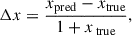 (2)
(2)where xtrue and xpred correspond to the true and predicted values, respectively.
-
Normalised median absolute deviation (NMAD): A robust statistic to measure scatter that is less sensitive to outliers. It is defined as
 (3)
(3) -
Outlier fraction: The fraction of predictions with |Δx| exceeding 0.15, and 0.25 for photo-z, and stellar mass, respectively, quantifying catastrophic prediction errors:
 (4)
(4)The choice of the threshold of 0.15 for photo-z is commonly used to define catastrophic outliers. For stellar mass, while no strict convention exists, a threshold of 0.25 corresponds to the standard stellar mass error (Siudek et al. 2024).
For binary classification tasks such as morphological classification (such as early-type versus late-type galaxies), we used the following metrics.
-
Accuracy: The proportion of correct predictions (both true positives and true negatives) among all predictions:
 (5)
(5)where NTP, NTN, NFP, and NFN are the number of true positives, true negatives, false positives, and false negatives, respectively.
-
Precision: The proportion of true positives among all instances predicted as positive:
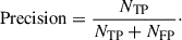 (6)
(6) -
Recall (true positive rate, TPR): The proportion of true positives among all actual positive instances:
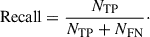 (7)
(7) -
False positive rate (FPR): The proportion of false positives among all actual negatives:
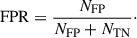 (8)
(8) -
F1 score: The harmonic mean of precision and recall, balancing the trade-off between them:
 (9)
(9)
4. Results
In this work, we explore the latent representations of galaxies derived from our pre-trained AstroPT models applied to three distinct datasets. The complementary nature of VIS, VIS + NISP, and VIS + NISP + SED data facilitates a systematic evaluation of the information content in the latent spaces derived from our models. This comparison also allows us to assess how well each wavelength constrains a galaxy’s physical parameters and to understand the limitations of relying solely on optical imaging.
4.1. AstroPT: Quality of self-supervised embeddings
In this section, we assess the quality and interpretability of self-supervised embeddings obtained from the Euclid VIS, VIS + NISP, and VIS + NISP + SED data via AstroPT. We do this by analysing their correlation with source properties. In all downstream tasks (including anomaly and similarity search, see Sect. 4.2), we used the raw 768-dimensional neural network embeddings as input. For visualisation purposes, we projected this high-dimensional embedding space onto two dimensions using uniform manifold approximation and projection (UMAP; McInnes et al. 2018). We initialised UMAP with a consistent set of hyperparameters for all visualisations (n_neighbours = 15, min_dist = 0.1, n_components = 2, random_state = 42) to ensure consistency across tasks. We validated different UMAP parametrisations, to: (i) determine whether the randomness in UMAP initialisation impacts the visualisations; (ii) to emphasize local structures that can potentially create tighter clusters; and (iii) to highlight the global relationships. While the shapes of the projections varied slightly across these settings, the trends related to galaxy morphological and physical properties remained consistent. Thus, we stuck to the default values that provide a good trade-off between the local, and global structures. The UMAP projection facilitates an intuitive exploration of clustering patterns and structures within the data. UMAP is particularly effective in preserving local and global structures, often outperforming methods such as principal component analysis (PCA) in revealing underlying relationships in the data (e.g. McInnes et al. 2018). However, we note that the dimensionality reduction algorithm ultimately influences the patterns and separations observed in these visualisations. While the UMAP projections suggest that relevant morphological and physical information is encoded in the AstroPT embeddings, the degree of separation achieved depends on the algorithm’s ability to preserve the global structure.
To more directly evaluate the utility of these embeddings, we also examined their performance in downstream tasks through approaches like the linear and MLP models (see Sect. 4.2). These analyses provide a complementary and quantitative assessment of the embeddings’ capacity to capture source properties, independent of the visualisation technique used.
A visualisation of the self-supervised embeddings trained on the VIS + NISP + SEDs images with example cut-outs and SEDs is shown in Fig. 6. The figure was created by binning the embedding space into a 50 × 50 grid and randomly selecting a sample from each cell, plotting its corresponding colour-mapped galaxy image at that location. The images were colour-mapped based on the VIS and NISP band images. The RGB image was generated only for visualisation purposes by averaging the YE-, JE-, and HE-band images to form an NISP channel, combining the VIS channel with this NISP channel to form a composite, and then stacking these three channels: VIS, NISP, and the composite. To preserve luminance, the luminosity channel of the resulting RGB image was replaced with the VIS channel, maintaining the brightness information while allowing for distinct colour contrasts. Zoom-in panels around the edges show that galaxies with similar morphologies tend to be clustered in different areas allowing for a separation of edge-on (left zoom-in panel), elliptical (top zoom-in panel), and spiral (bottom zoom-in panel) galaxies, while stars and low-quality images are separated in distinct cluster (right zoom-in panel). The zoom-in panels of spiral, and elliptical galaxies are selected within a photo-z range of 0.5 to 0.7, ensuring a fair comparison of their SEDs. While no striking differences are observed, the SEDs appear to broadly reflect morphological trends. Specifically, edge-on disc galaxies and ellipticals tend to be redder. However, this distinction is subtle and subject to interpretation. Additionally, the SEDs of stars and sources with lower data quality show spurious features. A similar plot, but generated using the AstroPT embeddings trained on VIS, and VIS + NISP data, is provided in Appendix B.
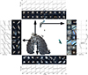 |
Fig. 6. UMAP visualisations of the embeddings from AstroPT trained on VIS + NISP + SEDs with example cut-outs and SEDs, see Sect. 4.1 for more details. |
The visual similarity of sources located close to each other in the representative space is also confirmed by their properties. The outlier regions are clearly separated from the main representations and are mostly attributed to bad-quality imaging and stars. Figure 7 shows the relationship between the embeddings trained on VIS images only, on VIS + NISP images, and VIS + NISP + SED, and the detection quality flag. The detection quality flag (DET_QUALITY_FLAG) is a flag indicating specific issues with sources, such as contamination, blending, or proximity to bright stars (Merlin et al. 2015, 2016, 2019; Kümmel et al. 2022). The UMAP projections reveal significant structure within the embedding space, reflecting the quality of the data: sources with high-quality images (DET_QUALITY_FLAG < 4) cluster tightly, whereas sources with contamination (e.g. blending or proximity to bright stars) form distinct outlier clusters. Including NISP data enhances the separation of poorly flagged sources, suggesting that NIR data provides complementary morphological information compared to VIS data. This improvement may arise because NIR observations are less affected by dust extinction and better trace the underlying stellar mass distribution, which can help distinguish extended or blended sources that are challenging to classify in VIS alone. In particular, embeddings trained on VIS + NISP images reveal two primary branches: one dominated by sources flagged as unknown (i.e. not fitting galaxy, star, or QSO templates); and another branch associated with sources of lower quality. However, the separation between galaxies, stars, and QSOs remains less defined (see details in Appendix C). When SED information is incorporated into the training (VIS + NISP + SED), the embeddings show a bimodal structure, which is driven by the spatial distribution: the EDF-N and EDF-S are targeted by different telescopes (see Sect. 2). Besides these two main branches, stars are also more distinctly separated, benefiting from the additional spectral information provided by SEDs. Furthermore, the unknown sources form a more coherent and distinguishable cluster, indicating that the combination of imaging and SED data aids in isolating these objects from other classes. This highlights the potential of SED data to complement imaging in disentangling complex or ambiguous cases, such as blended sources or objects with uncertain classifications.
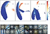 |
Fig. 7. Top: UMAP visualisations of the self-supervised embeddings from AstroPT trained on VIS (left), VIS + NISP (centre), and VIS + NISP + SED (right) images coloured by the detection quality flag. This flag allows one to identify sources with contaminants, e.g. proximity star (DET_QUALITY_FLAG ≥4). Bottom: Example VIS + NISP cut-outs of the outliers in the representative space. |
We also examined the correlation of the self-supervised embeddings with morphological parameters derived from the GZ catalogue (Euclid Collaboration: Walmsley et al. 2026b). Early-type galaxies typically exhibit smooth profiles, while late-type galaxies tend to show distinct features such as spiral arms or a bulging core, contributing to a more complex, less smooth morphology. Although not identical, the GZ classification between smooth and featured galaxies provided with the Euclid Q1 release (Euclid Collaboration: Walmsley et al. 2026b) closely approximates an early- and late-type separation. The UMAP visualisations reveal distinct clustering patterns that correspond to an early and late-type separation and the presence of spiral arms as shown in Fig. 8. Across all embeddings – whether AstroPT is trained on VIS, VIS + NISP, or VIS + NISP + SED – specific regions of the latent space are consistently associated with early-type galaxies, which also exhibit a low probability of hosting spiral arms. Conversely, other areas correspond to late-type galaxies with pronounced spiral structures. While the gradients within VIS + NISP + SED embeddings are clear, the separations between morphological types become harder to identify. This suggests that the embeddings prioritise spectral diversity over morphological clarity when SED data are included, highlighting a trade-off between the abstraction of spectral information and the preservation of morphological distinctions. This highlights the ability of automatic separation of elliptical and star-forming galaxy populations.
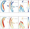 |
Fig. 8. UMAP visualisations of the self-supervised embeddings from AstroPT trained on VIS (left), VIS + NISP (centre), and VIS + NISP + SED (right) coloured by morphological parameters derived from the GZ catalogue (Euclid Collaboration: Walmsley et al. 2026b). Representations show clear clustering of smooth, non-spiral, and non-smooth, spiral galaxies. |
Interestingly, edge-on galaxies form a clearly identifiable region in the embeddings trained on VIS images alone, highlighting the capability of AstroPT to capture these specific morphological features (see the left panel in Fig. 9). This morphological distinctiveness aligns with their SED properties: a rising flux towards longer wavelengths, indicative of more dust, supports expectations for edge-on star-forming disc galaxies. However, as additional data from the NISP bands, and SEDs are incorporated, this distinct separation becomes less pronounced in the VIS + NISP and VIS + NISP + SED embeddings, as seen in the middle, and right panels of Fig. 9. While the inclusion of NISP and SED data enriches the latent space by providing additional spectral information, it does not necessarily enhance the clarity of morphological separations. Instead, the embeddings appear to encode a broader range of physical and morphological characteristics, becoming more abstract as additional data are integrated. The reduction in morphological separation, particularly for edge-on galaxies, may also be attributed to the lower resolution of NISP images relative to VIS, which limits the preservation of finer structural details. This does not imply that AstroPT’s performance degrades with lower-resolution data but instead highlights the trade-offs in representation fidelity when combining datasets of varying resolutions. These findings demonstrate the adaptability of AstroPT to encode rich, multidimensional information, albeit at the cost of losing some morphological specificity in certain contexts.
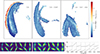 |
Fig. 9. UMAP visualisations of the self-supervised embeddings from AstroPt coloured by morphological parameters derived from the GZ catalogue (Euclid Collaboration: Walmsley et al. 2026b). Left: Representations from VIS images alone, showing a distinct region for edge-on galaxies. Middle: Representations incorporating both VIS and NISP data, where the separation of edge-on galaxies becomes less distinct. Right: Representations incorporating VIS, NISP, and SED data. Bottom: Example cut-outs and SEDs of the edge-on galaxies. |
Similarly, we find that physical properties are correlated with the latent space and morphological parameters. Namely, the region associated with spiral galaxies is characterised by lower stellar masses, while the space occupied by elliptical galaxies tends to have higher masses. There is though no trend with the Euclid spectroscopic redshift and only a subtle trend of higher redshift for more massive galaxies using photo-zs. More details are given in Appendix D.
These visualisations confirm that the self-supervised embeddings capture meaningful physical and morphological properties, with improved performance when both VIS and NISP data are utilised, except for the shape elongation (i.e. edge-on, ellipticity) which are caught by VIS embeddings but blended when using VIS + NISP imaging. The latent space’s ability to distinguish between low- and high-quality data, as well as between source types, underscores the robustness of the AstroPT framework for image analysis.
4.2. Downstream tasks
In our work, we evaluate the utility of self-supervised representations for different downstream tasks: morphology classification (see Sect. 4.2.1), photo-z estimations (see Sect. 4.2.2), and stellar mass predictions (see Sect. 4.2.3).
4.2.1. Morphological properties
The performance of three different methods – a supervised CNN, a linear model, and an MLP model (see Sect. 3.2) –is evaluated for their ability to classify galaxy as early-type or late-type based on the morphological catalogue (see Euclid Collaboration: Walmsley et al. 2026b). We define galaxies as early-type if the probability of being classified as smooth exceeds 0.5 and as late-type otherwise. However, this threshold-based classification may introduce inaccuracies, as it relies on predicted continuous probabilities rather than an inherent binary distinction. The accuracy, precision, and recall as a function of the percentage of labelled data are shown in Fig. 10. Table 3 shows a statistical summary for models trained on 100% of the labels, while Table E.1 extends this comparison across all percentages of labelled data. As expected, the results suggest that performance varies with the percentage of the labelled data used for training, but this dependence is neither uniform nor consistent across methods. In particular, the linear and MLP models present relatively stable performance, with only minor fluctuations, suggesting that even modest amounts of labelled data are sufficient for robust classification. However, the supervised CNN shows a more pronounced dependence on labelled data, with a clear decline in accuracy, precision, and recall as the labelled dataset size decreases. Interestingly, incorporating NISP imaging does not enhance classification performance; in some cases, it even slightly lowers accuracy, precision, and recall, possibly due to the NISP spatial resolution (see also discussion about edge-on galaxies in Sect. 4.1) or due to z-score normalisation (see Sect. 3). Similarly, adding SEDs does not improve classification, likely because the SEDs contain little direct morphological information. These findings suggest that while increasing the number of labelled examples provides some benefits, a self-supervised pre-training dramatically reduces the need for labelled samples. The self-supervised embeddings, trained on a relatively small labelled sample, already provide a robust foundation for morphological classification. Notably, the MLP model consistently achieves the highest performance across all metrics, particularly in distinguishing between early-type and late-type galaxies.
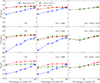 |
Fig. 10. Comparison of the accuracy, precision, and recall as functions of the percentage of labels used for training, for early-type/late-type classification. Results are shown for the VIS (left), VIS + NISP (centre), and VIS + NISP + SED configurations. |
Comparison of early- and late-type galaxy classification performance for different approaches.
4.2.2. Photometric redshifts
We verified the performance of different methods in predicting photo-z using the metrics described in Sect. 3.2. The spec-zs from DESI, available for about 5% of our sample, were assumed to be the true redshifts. The accuracy of Euclid photo-z derived with NNPZ as part of the Q1 release is shown in the top panel in Fig. 11. Figure 12 shows the bias, NMAD, and outlier fraction as a function of the percentage of labels used for training for photo-z obtained through these methods. A statistical summary is provided in Table 4 for a 100% of labels used for training, for the full table see Table E.2. The results highlight the impact of adding NISP imaging data, and SED information, and the effectiveness of different training approaches. The inclusion of NISP imaging improves photo-z accuracy, reducing metrics to levels comparable to those achieved by the official Euclid pipeline coming from the NNPZ template fitting algorithm (Euclid Collaboration: Tucci et al. 2026). These improvements are consistent with previous findings, such as those by Salvato et al. (2019), who demonstrated the importance of including NIR bands to constrain galaxy redshifts, particularly at higher redshifts. The performance is further improved when the SED information is included in the training. The bottom panel in Fig. 11 illustrates the ability of the MLP model to predict photo-zs, showing that the VIS + NISP + SED configuration achieves tighter clustering of predictions around the ideal 1:1 line, while the NNPZ photo-zs exhibit a more significant offset. Notably, the MLP model that catches the non-linearity tends to outperform other methods across all metrics, particularly for low percentages of labelled data. This approach achieves lower NMAD, and outlier fractions demonstrating its ability to adaptively leverage the added NISP, and SED information. For instance, with 100% labelled data, the MLP model achieves an NMAD = 0.048 ± 0.002 and an outlier fraction of 2.13 ± 0.38%, for training on VIS + NISP + SEDs approaching the performance of the official Euclid photo-z pipeline (NMAD = 0.037 and an outlier fraction of 2.21%). Linear models, while simpler, deliver competitive results for higher percentages of labelled data, where they approach the performance of Euclid pipeline, and more complex models. We note that we observe a non-monotonic behaviour in model performance as a function of training sample size. Specifically, the NMAD and outlier fraction peak at 5% training data, while performance improves at both smaller (1%) and larger (20%) sample sizes. This behaviour suggests the combination of the presence of the double descent effect (e.g. Schaeffer et al. 2023) in our regression model, and sample size balance. The double descent phenomenon occurs when test error initially decreases with increasing data size (classical regime), then spikes at an interpolation threshold, and finally decreases again as overparameterisation allows for better generalisation. In our case, with larger sample sizes (> 10%), the model moves into the overparameterised regime, where it can better capture meaningful patterns. On the other hand, when training on extremely limited data, the model may underfit, but given the low parameter count in linear regression this underfitting is less pronounced compared to the interpolation threshold. The fact that 1% performs comparably to 10% suggests that at extremely low sample sizes, the model is unable to overfit noise significantly, leading to stable results. In comparison, supervised CNN models exhibit modest improvements with increased labelled data, but generally underperform compared to other methods.
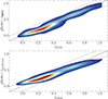 |
Fig. 11. Comparison of photo-z from Euclid official NNPZ pipeline (top) and predictions from the MLP model trained on AstroPT embeddings (bottom) versus DESI spec-z. A solid black line represents the 1:1 relation, while dotted lines indicate the outlier thresholds of 0.15. |
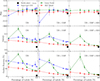 |
Fig. 12. Comparison of the bias, NMAD, and outlier fraction as functions of the percentage of labels used for training, for true redshift (DESI spec-z) versus Euclid photo-z predictions. Results are shown for the VIS (left), VIS + NISP (middle), and VIS + NISP + SED (right) configurations. |
Comparison of photo-z prediction performance for different approaches.
Overall, an MLP model trained with SED (VIS + NISP + SED data), not only achieves the best overall metrics, with improvements in bias and outlier fraction values in comparison to photo-zs from NNPZ for higher labelled data percentages, but also maintains superior results under low-data scenarios, demonstrating its robustness and adaptability for photo-z estimation tasks requiring only the SED information. These results underscore the effectiveness of leveraging advanced training strategies for accurate photometric redshift estimation.
4.2.3. Stellar masses
In this section we evaluated how AstroPT model is able to predict the stellar masses in comparison to more traditional approaches. As the ground truth, we assume the stellar masses of the DESI Value-Added Catalogue (Siudek et al. 2024), which provides a robust dataset derived from the SED fitting of optical and infrared photometry. First, we compare the stellar masses from Euclid official pipeline (Euclid Collaboration: Tucci et al. 2026) with the ones from DESI (see Fig. 13). The stellar masses are in agreement, as shown by the following 1:1 relation, but there is also a wide spread.
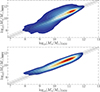 |
Fig. 13. Comparison of stellar mass from Euclid official NNPZ pipeline (top) and predictions from MLP model trained on AstroPT embeddings (bottom) versus DESI stellar masses from Siudek et al. (2024). A solid black line represents the 1:1 relation, while dotted lines indicate the outlier thresholds of 0.25 dex. |
Similarly, as for the morphological parameters and photo-zs, we predict stellar mass using different methods and metrics introduced in Sect. 3.2. We compare this property for both VIS and VIS + NISP models, but do not compare for our VIS + NISP + SED model as the z-score normalisation across the SEDs removes the additional information needed to predict this property. The bias, NMAD, and outlier fraction as a function of the percentage of labelled data for the stellar mass are shown in Fig. 14. A statistical summary is given in Table 5. The MLP model, and linear model consistently achieve the lowest NMAD across, but only MLP is independent on the number of labels used for training, demonstrating its robustness even with limited labelled data. The linear method, similarly to the photo-z estimates, shows the non-homogenous behaviour due to sample size, and the double descent effect (see Sect. 4.2.2 for details). Nevertheless, for all labels used in training, both linear and MLP methods outperform estimates from Euclid official pipeline when the AstroPT is trained on both VIS and NISP data. In particular, stellar mass predictions with the linear model are statistically even closer to DESI stellar masses than official NNPZ estimates (with NMAD 0.023 ± 0.001, and 0.027, and outlier fraction 0.3 ± 0.1%, 2.34% for MLP, and NNPZ, respectively. The performance degrades when solely VIS images are used for training. This highlights the added value of NISP’s complementary wavelength coverage in constraining stellar mass. The distributions of the MLP stellar mass predictions is shown in the bottom panel in Fig. 13.
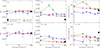 |
Fig. 14. Comparison of the NMAD and outlier fraction as functions of the percentage of labels used for training, for DESI stellar masses from Siudek et al. (2024) versus Euclid predictions. Results are shown for the VIS (left) and VIS + NISP (right) configurations. |
Comparison of stellar mass prediction performance for different approaches.
4.2.4. Anomaly search
To identify peculiar objects within the learned feature space, we applied two unsupervised anomaly detection algorithms – isolation forest (IF; Liu et al. 2008) and local outlier factor (LOF; Breunig et al. 2000) – to the AstroPT embeddings. Both methods were implemented using the Scikit-learn Python package (Pedregosa et al. 2011). Before running the algorithms, we filtered out spurious detections by removing sources with DET_QUALITY_FLAG > 0. To ensure robustness against sensitivity to parameter choices, we executed each algorithm multiple times with varying hyperparameters. Specifically, IF was tested with different numbers of base estimators, ranging from 50 to 200 in increments of 50, and the maximum number of features for splitting is varied between 1 and 20 in steps of 5. Additionally, we set the contamination parameter to an estimated fraction of outliers in the dataset and do not use bootstrap sampling. For LOF, we explored the effect of different neighbourhood sizes by varying the number of neighbours from 5 to 50 in steps of 5. We used the ‘ball-tree’ (Dolatshah et al. 2015) algorithm for nearest neighbour searches and employed the cosine distance metric, as it has been shown to better capture similarities in high-dimensional spaces (Aggarwal et al. 2001; You 2025). The contamination parameter is set to reflect the expected proportion of outliers.
In the embeddings trained solely with VIS images, LOF predominantly detects anomalies often associated with spurious features, such as cosmic rays, bright stars in close proximity, or ghost artefacts (see upper panel in Fig. 15). We note that these objects were not flagged by standard quality-control metrics, indicating LOF’s ability to identify subtle irregularities that might otherwise be overlooked. Additionally, LOF identifies extended objects in the outskirts of the cut-out region, sometimes galaxies located far from image centres. These galaxies tend to be brighter and more extended than the central source, though such cases are relatively rare since most relevant features are concentrated near the image centre. In contrast, IF predominantly identifies large galaxies with rich morphological structures, including those with prominent rings indicative of recent merger events (see lower panel in Fig. 15). A key distinction between the two methods emerges in the spatial distribution of detected anomalies within the embedding space: LOF-identified outliers are scattered throughout, whereas IF-detected anomalies cluster closely together in the latent space (see Fig. 16). These differences highlight the sensitivity of each method to different types of anomalies, with LOF favouring local density variations, and IF is adept at detecting sources with complex morphological structures.
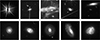 |
Fig. 15. Example VIS cut-outs of anomaly detections found with LOF (upper panel) and IF (bottom panel) on VIS embeddings. |
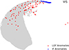 |
Fig. 16. UMAP visualisations of the self-supervised embeddings trained on VIS images with anomalies detected with LOF, and IF algorithms. |
When incorporating both VIS and NISP embeddings, the nature of the detected anomalies shifts. Both with IF and LOF algorithms, the VIS + NISP embedding highlights objects with multiple sources appearing within the field of view, potentially identifying interacting galaxies (see Fig. B.2). However, this embedding is also prone to contamination by non-interacting systems, as the algorithms do not inherently account for redshift differences and instead focus on structural features within the images. Including redshift information as an additional constraint within the anomaly detection process could help disentangle interacting systems from unrelated projections of nearby and distant galaxies. Alternatively, utilising smaller image cut-outs centred on each source might reduce confusion from neighbouring objects, improving both the accuracy and physical interpretability of detected anomalies. These refinements would enable a more reliable identification of astrophysically meaningful outliers within the embedding space.
When SED information is included, the nature of the detected anomalies changes once again. This exemplifies how complementary information can alter the structure of the embedding space and, consequently, the anomaly detection results. As more information is incorporated, anomalies become potentially more interesting. When using the IF algorithm, we detect objects with significant dust presence, predominantly in the HE band (see Fig. 17). The inclusion of SED data provides a measure of the relative importance of emission across different wavelengths, encoding valuable physical information. Interestingly, although the LOF algorithm still tends to detect anomalies driven by spurious features, it is nonetheless able to identify the two most prominent anomalies found with IF.
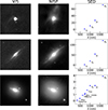 |
Fig. 17. Anomalies detected with the IF algorithm in the VIS + NISP + SED embedding. For each galaxy we show VIS and NSIP images and the SED. Fluxes are normalised to the Euclid VIS value. |
4.2.5. Similarity search
AstroPT projects objects with comparable features into the same regions of the embedding space, facilitating efficient similarity searches to identify objects of interest. This approach has shown great promise in various applications, particularly in identifying interacting galaxies. By using an interacting galaxy as a query, one can probe the embedding space to assess how many of its neighbouring galaxies also exhibit signs of interaction. This method allows for the rapid identification of potential interacting galaxies, contributing to large-scale surveys and studies of galaxy dynamics. In this work, we explore the potential of similarity search for identifying interacting galaxies and investigate how this approach can be adapted to astronomical datasets. As shown in Fig. 18, a significant fraction of the neighbouring galaxies to a query galaxy – chosen as an interacting galaxy – hereafter referred to as ‘similar objects’ – are indeed interacting. In particular, the distribution of the merging_merger parameter, which quantifies the probability of galaxies being in a merger process (Euclid Collaboration: Walmsley et al. 2026a), shows a higher fraction of merger candidates among the similar objects compared to the general galaxy population. This suggests that the similarity search effectively identifies galaxies involved in interactions. However, we also observe that the distribution of similar objects remains elongated, extending towards non-interacting galaxies as indicated by merging_merger ≈0, similar to the general distribution. This implies that, while the method is generally effective, it is not without contamination. In particular, the similarity search identifies some galaxies that are not truly interacting, highlighting the need for further refinement of the approach to reduce such false positives.
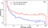 |
Fig. 18. Distribution of merging_merger parameter for similar objects computed with VIS embedding and general galaxy distribution. |
The presence of non-interacting neighbours, or ‘false positives’, in the identified clusters can be explained by the way AstroPT was trained and operates. During the training process, a fixed image size was chosen to ensure that the largest galaxies were fully captured within the image frame. This approach works well for galaxies at lower redshifts, where the central regions of galaxies can be clearly separated. However, for higher-redshift galaxies, the fixed image size may include multiple objects or extended outskirts of galaxies within the same frame. As a result, the algorithm may erroneously prioritise similarities in the outskirts of these galaxies, where there may be multiple objects or extended features, rather than focusing solely on the central regions where interactions are more likely to be detected. This can lead to the identification of objects as interacting when they are not, especially if the objects in question lie at different redshifts or are not truly interacting.
Despite these limitations, the approach shows great potential in identifying interacting galaxies. The contamination in the results, while non-negligible, offers insight into the nuances of the similarity search method and highlights the need for further refinement, particularly in distinguishing objects that are at different redshifts or in disentangling the central regions of interacting galaxies from their outskirts. These findings contribute to the broader understanding of similarity search applications in astrophysics and suggest areas for improvement in future models to enhance the accuracy of interaction detection.
5. Summary
In this paper, we have explored AstroPT, an autoregressive foundation model pre-trained on approximately 300 000 optical and infrared Q1 imaging and SEDs for deriving galaxy properties. By learning a unified and informative representation from multi-modal data, AstroPT provides a scalable solution for analysing large, unlabelled datasets, reducing dependence on human-labelled training samples while maintaining high performance for a variety of downstream tasks (such as photometric redshift estimation, morphology classification, anomaly detection).
The paper’s highlights are as follows.
-
Advancing foundation models in astronomy: AstroPT showcases the potential of multi-modal foundation models for a scalable and efficient resolution of many crucial astrophysical tasks, such as morphology classification, galaxy characterisation, and the search for peculiar sources. Unlike traditional task-specific models, AstroPT provides a generalisable feature space applicable across multiple domains, demonstrating the feasibility of self-supervised learning for astronomy at scale. Our results provide critical insight into the synergy between optical, infrared, and SED data, guiding future strategies for galaxy characterisation and cosmological analysis with Euclid.
-
Multi-modal synergies: The integration of optical, and NIR photometry highlights the advantages of multi-modal approaches. Pre-trained embeddings capture the inherent diversity of galaxy morphologies (see Figs. 6 and 8), clearly isolating galaxy classes hardly distinguishable with standard methods, such as edge-on galaxies (see Fig. 9), and outliers, such as spurious objects and stars missed by standard techniques (see Figs. 7 and C.1).
-
Unified representations for multiple tasks: Self-supervised embeddings provide a consistent representation for various downstream tasks, including photo-z and stellar mass estimates, anomalies, and similarity searches. This cross-task applicability underscores the flexibility of AstroPT’s learned representations, which remain effective across different astrophysical domains. By leveraging the task-agnostic nature of self-supervised embeddings, we reduce dependence on large labelled datasets while maintaining high performance. This scalability is crucial for addressing the challenges of analysing large multi-modal datasets in future surveys.
-
Morphological classification: Using solely optical images, our models achieve robust performance in predicting galaxy types. Surprisingly, incorporating NIR data and SEDs does not improve classification results, indicating that the additional spectral coverage does not introduce significant morphological information. The MLP and linear models demonstrate consistent performance across different dataset sizes, maintaining higher robustness compared to traditional supervised approaches, even with a limited number of labels (see Fig. 10 and Table 3). This suggests that deep-learning-based embeddings effectively capture morphological characteristics using only optical imaging, potentially simplifying future survey strategies.
-
Photo-z estimations: By integrating NIR, optical images, and SEDs, our models achieve competitive accuracy in photo-z estimates compared to the standard Euclid pipeline relying on traditional methods. Notably, the MLP model shows reduced bias and a lower fraction of catastrophic outliers, demonstrating that self-supervised embeddings can enhance photometric redshift predictions while being less reliant on large labelled training samples (see Fig. 12, and Table 4). This highlights the potential of deep-learning models adapted for standard tasks such as photo-z estimations, and the importance of multi-band photometry for capturing diverse galaxy properties and achieving higher precision.
-
Stellar mass estimations: We explore the ability of AstroPT to reconstruct fundamental galaxy properties, such as stellar mass, showing that MLP-based models achieve high accuracy even in low-label regimes. The linear model performs comparably well, showcasing the flexibility of the learned representations (see Fig. 14 and Table 5). This result highlights the robustness of self-supervised learning in deriving astrophysical parameters, even when traditional template-fitting approaches require extensive labelled training sets.
-
Outlier and similarity search: AstroPT’s anomaly and similarity search capabilities allow for the identification of rare astrophysical objects, including galaxies with rings, interacting systems, and other unusual morphologies. Including SEDs in training, we can also identify very dusty sources. This demonstrates the model’s utility in detecting previously overlooked populations in large-scale galaxy surveys, paving the way for new discoveries in Euclid and future astronomical datasets. This work underscores the transformative potential of combining multi-modal datasets, self-supervised learning, and foundation models for tackling large-scale challenges in galaxy analysis.
-
Limitations, and future perspectives: While AstroPT demonstrates strong performance across multiple tasks, some limitations remain. The reliance on pre-training with Q1 data means that domain adaptation might be required for different survey depths or observational conditions. Additionally, the current classification thresholds, and sample selection, could introduce selection biases, necessitating further refinement. Future work should explore strategies to mitigate these biases and improve generalisation to different datasets.
Acknowledgments
The Euclid Consortium acknowledges the European Space Agency and a number of agencies and institutes that have supported the development of Euclid, in particular the Agenzia Spaziale Italiana, the Austrian Forschungsförderungsgesellschaft funded through BMK, the Belgian Science Policy, the Canadian Euclid Consortium, the Deutsches Zentrum für Luft- und Raumfahrt, the DTU Space and the Niels Bohr Institute in Denmark, the French Centre National d’Etudes Spatiales, the Fundação para a Ciência e a Tecnologia, the Hungarian Academy of Sciences, the Ministerio de Ciencia, Innovación y Universidades, the National Aeronautics and Space Administration, the National Astronomical Observatory of Japan, the Netherlandse Onderzoekschool Voor Astronomie, the Norwegian Space Agency, the Research Council of Finland, the Romanian Space Agency, the State Secretariat for Education, Research, and Innovation (SERI) at the Swiss Space Office (SSO), and the United Kingdom Space Agency. A complete and detailed list is available on the Euclid web site (www.euclid-ec.org). This work has made use of the Euclid Quick Release Q1 data from the Euclid mission of the European Space Agency (ESA), 2025, https://doi.org/10.57780/esa-2853f3b. Based on data from UNIONS, a scientific collaboration using three Hawaii-based telescopes: CFHT, Pan-STARRS, and Subaru www.skysurvey.cc. Based on data from the Dark Energy Camera (DECam) on the Blanco 4-m Telescope at CTIO in Chile https://www.darkenergysurvey.org. DESI construction and operations is managed by the Lawrence Berkeley National Laboratory. This research is supported by the U.S. Department of Energy, Office of Science, Office of High-Energy Physics, under Contract No. DE–AC02–05CH11231, and by the National Energy Research Scientific Computing Center, a DOE Office of Science User Facility under the same contract. Additional support for DESI is provided by the U.S. National Science Foundation, Division of Astronomical Sciences under Contract No. AST-0950945 to the NSF’s National Optical-Infrared Astronomy Research Laboratory; the Science and Technology Facilities Council of the United Kingdom; the Gordon and Betty Moore Foundation; the Heising-Simons Foundation; the French Alternative Energies and Atomic Energy Commission (CEA); the National Council of Science and Technology of Mexico (CONACYT); the Ministry of Science and Innovation of Spain, and by the DESI Member Institutions. The DESI collaboration is honored to be permitted to conduct astronomical research on Iolkam Du’ag (Kitt Peak), a mountain with particular significance to the Tohono O’odham Nation. MHC and MS acknowledge support from the State Research Agency (AEIMCINN) of the Spanish Ministry of Science and Innovation under the grants “Galaxy Evolution with Artificial Intelligence” with reference PGC2018-100852-A-I00 and “BASALT” with reference PID2021-126838NBI00. MS acknowledges also support by the Polish National Agency for Academic Exchange (Bekker grant BPN/BEK/2021/1/00298/DEC/1). HDS acknowledges financial support by RyC2022-030469-I grant, funded by MCIN/AEI/10.13039/501100011033 and FSE+.
References
- Aggarwal, C. C., Hinneburg, A., & Keim, D. A. 2001, in Database Theory – ICDT 2001, eds. J. Van den Bussche, & V. Vianu (Berlin, Heidelberg: Springer), 420 [Google Scholar]
- Breunig, M. M., Kriegel, H.-P., Ng, R. T., & Sander, J. 2000, Proceedings of the 2000 ACM SIGMOD International Conference on Management of Data, SIGMOD ’00 (New York, NY, USA: Association for Computing Machinery), 93 [Google Scholar]
- Brown, T. B., Mann, B., Ryder, N., et al. 2020, ArXiv e-prints [arXiv:2005.14165] [Google Scholar]
- Bundy, K., Bershady, M. A., Law, D. R., et al. 2015, ApJ, 798, 7 [Google Scholar]
- Chen, T., Kornblith, S., Norouzi, M., & Hinton, G. 2020, ArXiv e-prints [arXiv:2002.05709] [Google Scholar]
- Cheng, T.-Y., Conselice, C. J., Aragón-Salamanca, A., et al. 2020, MNRAS, 493, 4209 [Google Scholar]
- Cheng, T.-Y., Huertas-Company, M., Conselice, C. J., et al. 2021, MNRAS, 503, 4446 [NASA ADS] [CrossRef] [Google Scholar]
- Chu, J., Tang, H., Xu, D., Lu, S., & Long, R. 2024, MNRAS, 528, 6354 [NASA ADS] [CrossRef] [Google Scholar]
- Cortes, C., Jackel, L. D., Solla, S. A., Vapnik, V., & Denker, J. S. 1993, Guide Proceedings (San Francisco, CA, USA: Morgan Kaufmann Publishers Inc.), 327 [Google Scholar]
- Dark Energy Survey Collaboration (Abbott, T., et al.) 2016, MNRAS, 460, 1270 [Google Scholar]
- DESI Collaboration (Abareshi, B., et al.) 2022, AJ, 164, 207 [NASA ADS] [CrossRef] [Google Scholar]
- DESI Collaboration (Adame, A. G., et al.) 2024a, AJ, 167, 62 [NASA ADS] [CrossRef] [Google Scholar]
- DESI Collaboration (Adame, A. G., et al.) 2024b, AJ, 168, 58 [NASA ADS] [CrossRef] [Google Scholar]
- Diaz, F., & Madaio, M. 2023, ArXiv e-prints [arXiv:2307.03201] [Google Scholar]
- Dolatshah, M., Hadian, A., & Minaei-Bidgoli, B. 2015, ArXiv e-prints [arXiv:1511.00628] [Google Scholar]
- Domínguez Sánchez, H., Huertas-Company, M., Bernardi, M., Tuccillo, D., & Fischer, J. L. 2018, MNRAS, 476, 3661 [Google Scholar]
- Domínguez Sánchez, H., Huertas-Company, M., Bernardi, M., et al. 2019, MNRAS, 484, 93 [Google Scholar]
- El-Nouby, A., Klein, M., Zhai, S., et al. 2024, ArXiv e-prints [arXiv:2401.08541] [Google Scholar]
- Euclid Collaboration (Desprez, G., et al.) 2020, A&A, 644, A31 [EDP Sciences] [Google Scholar]
- Euclid Collaboration (Schirmer, M., et al.) 2022, A&A, 662, A92 [NASA ADS] [CrossRef] [EDP Sciences] [Google Scholar]
- Euclid Collaboration (Bisigello, L., et al.) 2023, MNRAS, 520, 3529 [NASA ADS] [CrossRef] [Google Scholar]
- Euclid Collaboration (Humphrey, A., et al.) 2023, A&A, 671, A99 [NASA ADS] [CrossRef] [EDP Sciences] [Google Scholar]
- Euclid Collaboration (Aussel, B., et al.) 2024, A&A, 689, A274 [NASA ADS] [CrossRef] [EDP Sciences] [Google Scholar]
- Euclid Collaboration (Enia, A., et al.) 2024, A&A, 691, A175 [NASA ADS] [Google Scholar]
- Euclid Collaboration (Leuzzi, L., et al.) 2024, A&A, 681, A68 [NASA ADS] [CrossRef] [EDP Sciences] [Google Scholar]
- Euclid Collaboration (Cropper, M., et al.) 2025, A&A, 697, A2 [Google Scholar]
- Euclid Collaboration (Jahnke, K., et al.) 2025, A&A, 697, A3 [Google Scholar]
- Euclid Collaboration (Mellier, Y., et al.) 2025, A&A, 697, A1 [Google Scholar]
- Euclid Collaboration (Aussel, H., et al.) 2026, A&A, 711, A1 (Euclid Q1 SI) [Google Scholar]
- Euclid Collaboration (Enia, A., et al.) 2026, A&A, 711, A14 (Euclid Q1 SI) [Google Scholar]
- Euclid Collaboration (McCracken, H. J., et al.) 2026, A&A, 711, A2 (Euclid Q1 SI) [Google Scholar]
- Euclid Collaboration (Polenta, G., et al.) 2026, A&A, 711, A3 (Euclid Q1 SI) [Google Scholar]
- Euclid Collaboration (Romelli, E., et al.) 2026, A&A, 711, A4 (Euclid Q1 SI) [Google Scholar]
- Euclid Collaboration (Tucci, M., et al.) 2026, A&A, 711, A5 (Euclid Q1 SI) [Google Scholar]
- Euclid Collaboration (Walmsley, M., et al.) 2026a, A&A, 711, A26 (Euclid Q1 SI) [Google Scholar]
- Euclid Collaboration (Walmsley, M., et al.) 2026b, A&A, 711, A9 (Euclid Q1 SI) [Google Scholar]
- Euclid Quick Release Q1. 2025, https://doi.org/10.57780/esa-2853f3b [Google Scholar]
- Fotopoulou, S. 2024, Astron. Comput., 48, 100851 [Google Scholar]
- Fukushima, K. 1980, Biol. Cybern., 36, 193 [CrossRef] [PubMed] [Google Scholar]
- Gai, M., Bove, M., Bonetta, G., Zago, D., & Cancelliere, R. 2024, MNRAS, 532, 1391 [Google Scholar]
- Grattafiori, A., Dubey, A., Jauhri, A., et al. 2024, ArXiv e-prints [arXiv:2407.21783] [Google Scholar]
- Gunn, J. E., Carr, M., Rockosi, C., et al. 1998, AJ, 116, 3040 [NASA ADS] [CrossRef] [Google Scholar]
- Gunn, J. E., Siegmund, W. A., Mannery, E. J., et al. 2006, AJ, 131, 2332 [NASA ADS] [CrossRef] [Google Scholar]
- Hayat, M. A., Stein, G., Harrington, P., Lukić, Z., & Mustafa, M. 2021, ApJ, 911, L33 [NASA ADS] [CrossRef] [Google Scholar]
- Henighan, T., Kaplan, J., Katz, M., et al. 2020, ArXiv e-prints [arXiv:2010.14701.] [Google Scholar]
- Hocking, A., Geach, J. E., Sun, Y., & Davey, N. 2018, MNRAS, 473, 1108 [CrossRef] [Google Scholar]
- Hoffmann, J., Borgeaud, S., Mensch, A., et al. 2022, ArXiv e-prints [arXiv:2203.15556] [Google Scholar]
- Huber, P. J. 1964, Ann. Math. Stat., 35, 73 [CrossRef] [Google Scholar]
- Huertas-Company, M., & Lanusse, F. 2023, PASA, 40, e001 [NASA ADS] [CrossRef] [Google Scholar]
- Huertas-Company, M., Iyer, K. G., Angeloudi, E., et al. 2024, A&A, 685, A48 [NASA ADS] [CrossRef] [EDP Sciences] [Google Scholar]
- Ivezić, Ž., Kahn, S. M., Tyson, J. A., et al. 2019, ApJ, 873, 111 [Google Scholar]
- Kaplan, J., McCandlish, S., Henighan, T., et al. 2020, ArXiv e-prints [arXiv:2001.08361] [Google Scholar]
- Kümmel, M., Álvarez-Ayllón, A., Bertin, E., et al. 2022, ArXiv e-prints [arXiv:2212.02428] [Google Scholar]
- Laureijs, R., Amiaux, J., Arduini, S., et al. 2011, ArXiv e-prints [arXiv:1110.3193] [Google Scholar]
- Liu, F. T., Ting, K. M., & Zhou, Z.-H. 2008, 2008 Eighth IEEE International Conference on Data Mining, 413 [Google Scholar]
- Loshchilov, I., & Hutter, F. 2017, ArXiv e-prints [arXiv:1711.05101] [Google Scholar]
- Mampaso, A., García de la Rosa, I., Arias, P., et al. 2022, Study on Environmental Sustainability at the Instituto de Astrofísica de Canarias and Proposed Actions, Technical Report, Instituto de Astrofísica de Canarias [Google Scholar]
- Martínez-Solaeche, G., García-Benito, R., González Delgado, R. M., et al. 2024, A&A, 688, A160 [NASA ADS] [CrossRef] [EDP Sciences] [Google Scholar]
- McInnes, L., Healy, J., & Melville, J. 2018, ArXiv e-prints [arXiv:1802.03426] [Google Scholar]
- Merlin, E., Fontana, A., Ferguson, H. C., et al. 2015, A&A, 582, A15 [NASA ADS] [CrossRef] [EDP Sciences] [Google Scholar]
- Merlin, E., Amorín, R., Castellano, M., et al. 2016, A&A, 590, A30 [NASA ADS] [CrossRef] [EDP Sciences] [Google Scholar]
- Merlin, E., Pilo, S., Fontana, A., et al. 2019, A&A, 622, A169 [NASA ADS] [CrossRef] [EDP Sciences] [Google Scholar]
- Merz, G., Liu, X., Schmidt, S., et al. 2025, Open J. Astrophys., 8, 40 [Google Scholar]
- Mishra-Sharma, S., Song, Y., & Thaler, J. 2024, ArXiv e-prints [arXiv:2403.08851] [Google Scholar]
- Mohale, K., & Lochner, M. 2024, MNRAS, 530, 1274 [NASA ADS] [CrossRef] [Google Scholar]
- Muennighoff, N., Rush, A. M., Barak, B., et al. 2023, ArXiv e-prints [arXiv:2305.16264] [Google Scholar]
- Nair, V., & Hinton, G. E. 2010, Proceedings of the 27th International Conference on International Conference on Machine Learning, ICML’10 (Madison, WI, USA: Omnipress), 807 [Google Scholar]
- Pan, J.-S., Ting, Y.-S., Huang, Y., Yu, J., & Liu, J.-F. 2024, ArXiv e-prints [arXiv:2405.17156] [Google Scholar]
- Parker, L., Lanusse, F., Golkar, S., et al. 2024, MNRAS, 531, 4990 [Google Scholar]
- Pattnaik, R., Kartaltepe, J. S., & Binu, C. 2025, ApJ, submitted [arXiv:2501.01070] [Google Scholar]
- Pedregosa, F., Varoquaux, G., Gramfort, A., et al. 2011, J. Mach. Learn. Res., 12, 2825 [Google Scholar]
- Radford, A., Kim, J. W., Hallacy, C., et al. 2021, International Conference on Machine Learning (PMLR), 8748 [Google Scholar]
- Rizhko, M., & Bloom, J. S. 2025, AJ, 170, 28 [Google Scholar]
- Rosenblatt, F. 1958, Psychol. Rev., 65, 386 [CrossRef] [Google Scholar]
- Salvato, M., Ilbert, O., & Hoyle, B. 2019, Nature, 3, 212 [Google Scholar]
- Sarmiento, R., Huertas-Company, M., Knapen, J. H., et al. 2021, ApJ, 921, 177 [NASA ADS] [CrossRef] [Google Scholar]
- Schaeffer, R., Khona, M., Robertson, Z., et al. 2023, ArXiv e-prints [arXiv:2303.14151] [Google Scholar]
- Sengupta, A., Goel, Y., & Chakraborty, T. 2025, ArXiv e-prints [arXiv:2505.00985] [Google Scholar]
- Siudek, M., Pucha, R., Mezcua, M., et al. 2024, A&A, 691, A308 [NASA ADS] [CrossRef] [EDP Sciences] [Google Scholar]
- Slijepcevic, I. V., Scaife, A. M. M., Walmsley, M., et al. 2024, RASTI, 3, 19 [Google Scholar]
- Smith, M. J., & Geach, J. E. 2023, R. Soc. Open Sci., 10, 221454 [NASA ADS] [CrossRef] [Google Scholar]
- Smith, M. J., Roberts, R. J., Angeloudi, E., & Huertas-Company, M. 2024, ArXiv e-prints [arXiv:2405.14930] [Google Scholar]
- Stein, G., Harrington, P., Blaum, J., Medan, T., & Lukic, Z. 2021, ArXiv e-prints [arXiv:2110.13151] [Google Scholar]
- Strubell, E., Ganesh, A., & Mccallum, A. 2019, ACL Anthology, 3645 [Google Scholar]
- Tanaka, M., Coupon, J., Hsieh, B.-C., et al. 2018, PASJ, 70, S9 [Google Scholar]
- The Multimodal Universe Collaboration (Audenaert, J., et al.) 2024, ArXiv e-prints [arXiv:2412.02527] [Google Scholar]
- Vega-Ferrero, J., Domínguez Sánchez, H., Bernardi, M., et al. 2021, MNRAS, 506, 1927 [NASA ADS] [CrossRef] [Google Scholar]
- Vega-Ferrero, J., Huertas-Company, M., Costantin, L., et al. 2024, ApJ, 961, 51 [NASA ADS] [CrossRef] [Google Scholar]
- Walmsley, M., Lintott, C., Géron, T., et al. 2022a, MNRAS, 509, 3966 [Google Scholar]
- Walmsley, M., Scaife, A. M. M., Lintott, C., et al. 2022b, MNRAS, 513, 1581 [NASA ADS] [CrossRef] [Google Scholar]
- Walmsley, M., Géron, T., Kruk, S., et al. 2023, MNRAS, 526, 4768 [Google Scholar]
- Walmsley, M., Bowles, M., Scaife, A. M. M., et al. 2024, ArXiv e-prints [arXiv:2404.02973] [Google Scholar]
- Xu, B., Wang, N., Chen, T., & Li, M. 2015, ArXiv e-prints [arXiv:1505.00853] [Google Scholar]
- You, K. 2025, ArXiv e-prints [arXiv:2504.16318] [Google Scholar]
- Zhang, G., Helfer, T., Gagliano, A. T., Mishra-Sharma, S., & Ashley Villar, V. 2024, Mach. Learn.: Sci. Technol., 5, 045069 [Google Scholar]
Appendix A: Hyperparameters, computations, and carbon emissions
The training of deep-learning models requires considerable energy, which can contribute to carbon emissions. To counteract further emission from unnecessary retraining we follow the recommendations of (Strubell et al. 2019) and make available our model weights and inference code in the Hugging Face repository4. While this study made use of the 100% renewable energy-powered ITER Teide HPC cluster (Mampaso et al. 2022) for pre-training, for the sake of transparency we estimate and show our energy usage during the pre-training of AstroPT here: AstroPT-90M takes 2 hours to train on 4xA100-40G NVIDIA GPUs, which corresponds to 2 kWh of energy use according to the Machine Learning CO2 Impact Calculator (https://mlco2.github.io/impact/).
Hyperparameters used in pre-training AstroPT-90M.
Appendix B: AstroPT embeddings for VIS and VIS+NISP imaging
Figure B.1 presents a visualisation of the AstroPT embeddings trained on the VIS (left) and combined VIS and NISP data (right). This plot demonstrates how the inclusion of both optical and infrared wavelengths influences the organisation and clustering of different galaxy types and stars in the embedding space.
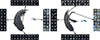 |
Fig. B.1. UMAP visualisations of the embeddings from AstroPT trained on VIS (left) and VIS+NISP (right) images with example cut-outs, see text for more details. |
In Fig. B.2, we show typical anomalies found with LOF (upper panel) and IF (bottom panel) for the VIS+NISP embedding. As can be observed, anomalies consist of images that include multiple objects within the cut-outs.
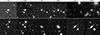 |
Fig. B.2. Example VIS and NISP cut-outs of anomaly detections found on VIS+NISP embeddings with IF (upper panel) and LOF (bottom panel). |
Appendix C: Star-QSO-galaxy separation
Figure C.1 shows the correlation of the embeddings with the source type (unknown, galaxy, star, QSO) derived from the spectroscopic pipeline. Clearly, the outlier regions of embeddings are occupied by stars and unknown sources, but stars are also found over all regions (see Fig. C.1). Galaxies, QSOs, and stars tend to occupy a broad distribution. Adding NISP data sharpens the separation of unknown objects where a long tail gathers the invalid NISP data. Incorporating SEDs further enhance the separation of unknown sources from the main space.
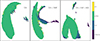 |
Fig. C.1. UMAP visualisations of the self-supervised embeddings from AstroPT coloured by the source type (QSO, galaxy, star, or unknown). The left panel corresponds to VIS-only embeddings, the centre panel includes both VIS and NISP data, and the right panel includes VIS, NISP, and SED data. |
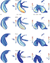 |
Fig. C.2. UMAP visualisations of the self-supervised embeddings from AstroPT. Top: Coloured by the stars. Bottom: Coloured by QSO. Left panels correspond to VIS-only embeddings, centre panels include both VIS, and NISP data, and the right panels include VIS, NISP, and SED data. |
Appendix D: Quality of the embeddings: Physical properties
Figures D.1, and D.2 highlight the relationship between the latent space and physical properties, such as stellar mass, and redshift. There is a clear connection between morphological trends (see Fig. 8) and stellar masses. Early-type galaxies, which are typically more massive, occupy regions of the UMAP space associated with higher stellar masses. In contrast, spiral galaxies, known for their lower stellar masses, cluster in distinct, separate regions. This differentiation is especially pronounced when embeddings are trained with VIS+NISP data, suggesting that the additional NISP features help to better constrain stellar mass distributions. This is further enhanced when the SEDs are included in the training. The Euclid photometric redshift shows no strong correlation with the embeddings, although there is a subtle trend of higher stellar masses being linked to slightly higher redshifts, especially for VIS+NIS+SED, consistent with the evolutionary connection between galaxy mass and formation epoch. The trend with the redshift is clearer when the spectroscopic redshift from DESI is used. These results underscore the utility of self-supervised representations in capturing key physical galaxy properties, particularly with multi-band data.
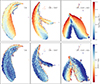 |
Fig. D.1. UMAP visualisation of self-supervised embeddings, highlighting correlations with stellar mass and photometric redshift. The left panels show the distribution of galaxies when AstroPT is trained on VIS images, while the centre panels represent the training with VIS+NISP images, and the right panels correspond to training on VIS, NISP images, and SEDs. The top UMAP visualisations are colour-coded by stellar mass from Euclid official pipeline (top). The bottom UMAP visualisations are colour-coded by Euclid official photometric redshifts. |
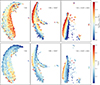 |
Fig. D.2. UMAP visualisation of self-supervised embeddings, highlighting correlations with stellar mass and photometric redshift. The left panels show the distribution of galaxies when AstroPT is trained on VIS images, while the centre panels represent the training with VIS+NISP images, and the right panels correspond to training on VIS, NISP images, and SEDs. The left UMAP visualisations are colour-coded by stellar mass from DESI VAC (Siudek et al. 2024). The right UMAP visualisations are colour-coded by the DESI spectroscopic redshift (DESI Collaboration 2024b) available for about 5% of the sample. |
Appendix E: Accuracy of predictions
Table E.1, E.2, and E.3 provide a detailed summary of the performance metrics for morphology classification, photo-z, and stellar mass predictions, respectively, across different models and data configurations (see Sect. 3.2). Metrics are reported for various percentages of labelled data used during training. These tables complements Figs. 10, 12, 14 by offering a more detailed view of the performance differences between the models. MLP model consistently achieves the best overall metrics, particularly when leveraging self-supervised embeddings with even a minimal set of labels. The linear model also demonstrates competitive performance, and serves as a robust baseline for comparison.
Comparison of early-type/late-type galaxy classification performance for different approaches. Results are reported for different percentages of labelled data used for training (1%, 5%, 10%, 50%, 80%, and 100%).
Comparison of photo-z prediction performance for different approaches. Results are reported for different percentages of labelled data used for training (1%, 5%, 10%, 50%, 80%, and 100%).
Comparison of stellar mass prediction performance for different approaches. Results are reported for different percentages of labelled data used for training (1%, 10%, 50%, 80%, and 100%).
All Tables
Photometric bands, instruments, observed depths, and fields included in the Euclid photometric catalogue used to build the SEDs of Q1 sources.
Comparison of different methodologies for regression and classification downstream tasks.
Comparison of early- and late-type galaxy classification performance for different approaches.
Comparison of early-type/late-type galaxy classification performance for different approaches. Results are reported for different percentages of labelled data used for training (1%, 5%, 10%, 50%, 80%, and 100%).
Comparison of photo-z prediction performance for different approaches. Results are reported for different percentages of labelled data used for training (1%, 5%, 10%, 50%, 80%, and 100%).
Comparison of stellar mass prediction performance for different approaches. Results are reported for different percentages of labelled data used for training (1%, 10%, 50%, 80%, and 100%).
All Figures
|
Fig. 1. Scaling laws for foundation models in astronomy compared to the GPT series. The number of tokens is defined as subword units in text (GPT models); pairs of augmented images (contrastive learning models); or a number of patches (AstroPT model). The projected scaling of future models incorporating Euclid data in upcoming data releases are marked with green stars. Our current model, trained on Q1 Euclid data, is represented by a red star. The models from the literature are referenced as follows: AH21 (Hayat et al. 2021); S21 (Sarmiento et al. 2021), GS21 (Stein et al. 2021); GMS24 (Martínez-Solaeche et al. 2024); P24 (Parker et al. 2024); and MS24 (Smith et al. 2024). |
| In the text | |
|
Fig. 2. Stellar mass-redshift relation for the Q1 sample (in cyan), the sample used in this work (in navy blue), and our sample with DESI spectroscopic information (in red). The inset plots show the residuals of redshift and stellar mass differences between the Euclid pipeline and DESI, respectively. |
| In the text | |
|
Fig. 3. Distribution of Euclid photometry for the sample used in this paper. |
| In the text | |
|
Fig. 4. Representative SEDs of galaxies from the Q1 EDF-N (top) and EDF-S fields (bottom). The SED includes multi-wavelength photometric data spanning the ultraviolet to the near-infrared listed in Table 1. |
| In the text | |
|
Fig. 5. AstroPT’s training objective is predicting the next patch in a sequence of galaxy image (and other modalities’) patches. On the left we show the order of galaxy patches used in this work, and on the right we show how each patch is processed by AstroPT. |
| In the text | |
|
Fig. 6. UMAP visualisations of the embeddings from AstroPT trained on VIS + NISP + SEDs with example cut-outs and SEDs, see Sect. 4.1 for more details. |
| In the text | |
|
Fig. 7. Top: UMAP visualisations of the self-supervised embeddings from AstroPT trained on VIS (left), VIS + NISP (centre), and VIS + NISP + SED (right) images coloured by the detection quality flag. This flag allows one to identify sources with contaminants, e.g. proximity star (DET_QUALITY_FLAG ≥4). Bottom: Example VIS + NISP cut-outs of the outliers in the representative space. |
| In the text | |
|
Fig. 8. UMAP visualisations of the self-supervised embeddings from AstroPT trained on VIS (left), VIS + NISP (centre), and VIS + NISP + SED (right) coloured by morphological parameters derived from the GZ catalogue (Euclid Collaboration: Walmsley et al. 2026b). Representations show clear clustering of smooth, non-spiral, and non-smooth, spiral galaxies. |
| In the text | |
|
Fig. 9. UMAP visualisations of the self-supervised embeddings from AstroPt coloured by morphological parameters derived from the GZ catalogue (Euclid Collaboration: Walmsley et al. 2026b). Left: Representations from VIS images alone, showing a distinct region for edge-on galaxies. Middle: Representations incorporating both VIS and NISP data, where the separation of edge-on galaxies becomes less distinct. Right: Representations incorporating VIS, NISP, and SED data. Bottom: Example cut-outs and SEDs of the edge-on galaxies. |
| In the text | |
|
Fig. 10. Comparison of the accuracy, precision, and recall as functions of the percentage of labels used for training, for early-type/late-type classification. Results are shown for the VIS (left), VIS + NISP (centre), and VIS + NISP + SED configurations. |
| In the text | |
|
Fig. 11. Comparison of photo-z from Euclid official NNPZ pipeline (top) and predictions from the MLP model trained on AstroPT embeddings (bottom) versus DESI spec-z. A solid black line represents the 1:1 relation, while dotted lines indicate the outlier thresholds of 0.15. |
| In the text | |
|
Fig. 12. Comparison of the bias, NMAD, and outlier fraction as functions of the percentage of labels used for training, for true redshift (DESI spec-z) versus Euclid photo-z predictions. Results are shown for the VIS (left), VIS + NISP (middle), and VIS + NISP + SED (right) configurations. |
| In the text | |
|
Fig. 13. Comparison of stellar mass from Euclid official NNPZ pipeline (top) and predictions from MLP model trained on AstroPT embeddings (bottom) versus DESI stellar masses from Siudek et al. (2024). A solid black line represents the 1:1 relation, while dotted lines indicate the outlier thresholds of 0.25 dex. |
| In the text | |
|
Fig. 14. Comparison of the NMAD and outlier fraction as functions of the percentage of labels used for training, for DESI stellar masses from Siudek et al. (2024) versus Euclid predictions. Results are shown for the VIS (left) and VIS + NISP (right) configurations. |
| In the text | |
|
Fig. 15. Example VIS cut-outs of anomaly detections found with LOF (upper panel) and IF (bottom panel) on VIS embeddings. |
| In the text | |
|
Fig. 16. UMAP visualisations of the self-supervised embeddings trained on VIS images with anomalies detected with LOF, and IF algorithms. |
| In the text | |
|
Fig. 17. Anomalies detected with the IF algorithm in the VIS + NISP + SED embedding. For each galaxy we show VIS and NSIP images and the SED. Fluxes are normalised to the Euclid VIS value. |
| In the text | |
|
Fig. 18. Distribution of merging_merger parameter for similar objects computed with VIS embedding and general galaxy distribution. |
| In the text | |
|
Fig. B.1. UMAP visualisations of the embeddings from AstroPT trained on VIS (left) and VIS+NISP (right) images with example cut-outs, see text for more details. |
| In the text | |
|
Fig. B.2. Example VIS and NISP cut-outs of anomaly detections found on VIS+NISP embeddings with IF (upper panel) and LOF (bottom panel). |
| In the text | |
|
Fig. C.1. UMAP visualisations of the self-supervised embeddings from AstroPT coloured by the source type (QSO, galaxy, star, or unknown). The left panel corresponds to VIS-only embeddings, the centre panel includes both VIS and NISP data, and the right panel includes VIS, NISP, and SED data. |
| In the text | |
|
Fig. C.2. UMAP visualisations of the self-supervised embeddings from AstroPT. Top: Coloured by the stars. Bottom: Coloured by QSO. Left panels correspond to VIS-only embeddings, centre panels include both VIS, and NISP data, and the right panels include VIS, NISP, and SED data. |
| In the text | |
|
Fig. D.1. UMAP visualisation of self-supervised embeddings, highlighting correlations with stellar mass and photometric redshift. The left panels show the distribution of galaxies when AstroPT is trained on VIS images, while the centre panels represent the training with VIS+NISP images, and the right panels correspond to training on VIS, NISP images, and SEDs. The top UMAP visualisations are colour-coded by stellar mass from Euclid official pipeline (top). The bottom UMAP visualisations are colour-coded by Euclid official photometric redshifts. |
| In the text | |
|
Fig. D.2. UMAP visualisation of self-supervised embeddings, highlighting correlations with stellar mass and photometric redshift. The left panels show the distribution of galaxies when AstroPT is trained on VIS images, while the centre panels represent the training with VIS+NISP images, and the right panels correspond to training on VIS, NISP images, and SEDs. The left UMAP visualisations are colour-coded by stellar mass from DESI VAC (Siudek et al. 2024). The right UMAP visualisations are colour-coded by the DESI spectroscopic redshift (DESI Collaboration 2024b) available for about 5% of the sample. |
| In the text | |
Current usage metrics show cumulative count of Article Views (full-text article views including HTML views, PDF and ePub downloads, according to the available data) and Abstracts Views on Vision4Press platform.
Data correspond to usage on the plateform after 2015. The current usage metrics is available 48-96 hours after online publication and is updated daily on week days.
Initial download of the metrics may take a while.