


| Issue |
A&A
Volume 710, June 2026
|
|
|---|---|---|
| Article Number | A194 | |
| Number of page(s) | 25 | |
| Section | Planets, planetary systems, and small bodies | |
| DOI | https://doi.org/10.1051/0004-6361/202659683 | |
| Published online | 12 June 2026 | |
Mitigating stellar radial velocity jitter using orthogonal activity indices and a time-aware neural network
1
Institut de Ciències de l’Espai (ICE, CSIC),
Campus UAB, Carrer de Can Magrans s/n,
08193
Bellaterra,
Spain
2
Institut d’Estudis Espacials de Catalunya (IEEC), Edifici RDIT,
Campus UPC,
08860
Castelldefels,
Barcelona,
Spain
3
Facultat de Física, Universitat de Barcelona (UB),
Martí Franquès 1,
08028,
Barcelona,
Spain
4
Department of Physics, University of Warwick,
Gibbet Hill Road,
Coventry
CV4 7AL,
UK
5
Centre for Exoplanets and Habitability, University of Warwick,
Coventry
CV4 7AL,
UK
6
Delft University of Technology, Department of Imaging Physics,
Gebouw 22, Lorentzweg 1,
2628 CJ
Delft,
The Netherlands
7
Data Science Center, Barcelona School of Economics,
Ramon Trias-Fargas 25-27,
08005
Barcelona,
Spain
★ Corresponding author: This email address is being protected from spambots. You need JavaScript enabled to view it.
Received:
3
March
2026
Accepted:
30
April
2026
Abstract
Context. Despite recent advances in the precision of high-resolution spectrographs, the detection of Earth-like exoplanets is still limited by the effects of stellar activity, which introduce radial velocity variations at the metre-per-second level or larger.
Aims. We present a framework to disentangle stellar effects from planetary signals by exploiting high-order distortions of the cross-correlation function (CCF; a measure of the average spectral line profile), thus moving beyond the commonly applied Gaussian fit approximation.
Methods. We decomposed the CCF using a Gram–Schmidt orthogonal basis function, enabling the separation of pure line shifts from line-shape distortions. To model activity-induced contributions to the radial velocities, we have developed a time-aware convolutional attention network dubbed CANSTAR. This network was trained on synthetic line-shape distortion coefficients produced with the realistic stellar simulator StarSim to learn the temporal evolution of stellar activity features.
Results. We validated our framework using HARPS and CARMENES observations of two active stars, ϵ Eridani and TZ Arietis. The network effectively mitigates stellar activity, reducing the radial velocity RMS to 52.5% and 62.4% of the uncorrected variability, respectively. This correction enables a more precise determination of the orbital parameters of TZ Arietis b compared to a Gaussian process regression.
Conclusions. Our results demonstrate that neural networks that incorporate the temporal context can outperform state-of-the-art methods in complex activity regimes. Future improvements on StarSim that will allow us to train CANSTAR on 3D magnetohydrodynamic spectra and more complex instrumental modelling are expected to bridge the performance gap between synthetic and real data, offering a robust pathway towards detecting Earth-mass planets around Sun-like stars.
Key words: methods: data analysis / techniques: radial velocities / planets and satellites: detection / stars: activity / stars: individual: e Eridani / stars: individual: TZ Arietis
© The Authors 2026
 Open Access article, published by EDP Sciences, under the terms of the Creative Commons Attribution License (https://creativecommons.org/licenses/by/4.0), which permits unrestricted use, distribution, and reproduction in any medium, provided the original work is properly cited.
This article is published in open access under the Subscribe to Open model. This email address is being protected from spambots. You need JavaScript enabled to view it. to support open access publication.
1 Introduction
Since the discovery of 51 Pegasi b in 1995 (Mayor & Queloz 1995), the radial velocity (RV) method has allowed for the detection of over a thousand exoplanets, moving over time from large Jupiter-like planets to smaller rocky worlds orbiting in the temperate zone of their host stars (e.g. Hatzes et al. 2000; McArthur et al. 2004; Anglada-Escudé et al. 2016). This progress has been largely due to technical improvements on spectrographs, which have gradually pushed detection limits from signals in the tens of metres per second down to the m s−1 domain, with instruments such as HARPS (Mayor et al. 2003), HARPS-N (Cosentino et al. 2012), CARMENES (Quirrenbach et al. 2016), and SPIRou (Donati et al. 2018). The newest spectrographs, for example, ESPRESSO (Pepe et al. 2010), with an instrumental precision reaching down to around 10 cm s−1, represent a big leap towards the detection of even smaller Keplerian signals induced by Earth-like rocky planets (Figueira et al. 2025).
Despite these instrumental advancements, stellar magnetic activity remains a fundamental barrier to detecting low-amplitude RV signals. Surface inhomogeneities such as spots, faculae, and granulation can induce RV variations greater than 1 m s−1, even in relatively quiet stars (e.g. Dumusque et al. 2012; Perger et al. 2017). These stellar activity effects distort spectral line shapes, potentially mimicking or obscuring planetary signals. The two main RV extraction methods are affected by these wavelength-dependent distortions, and the community has developed different strategies for each technique to disentangle planetary signals from instrumental or stellar activity variability.
In the cross-correlation function (CCF) method, the observed spectrum is cross-correlated with a weighted mask tailored to the stellar spectral type (Baranne et al. 1996). The resulting CCF represents an average stellar absorption line. For most stars, the CCF is well described by a Gaussian profile. The centroid yields the RV, while the contrast (CON) and the full width at half maximum ( , where σ2 is the variance of the Gaussian) are line-shape activity indicators. The bisector inverse slope (BIS), defined as the velocity difference between the upper (60–90%) and lower (10–40%) parts of the CCF, is used as a measurement of line asymmetry (Queloz et al. 2001). Several alternative approaches have been developed to extract activity information from the CCF, including bi-Gaussian fitting with asymmetric widths (Figueira et al. 2013), Fourier decomposition (Zhao & Tinney 2020), principal component analysis (PCA) of the auto-correlation function (Collier Cameron et al. 2021), and PCA on shape-driven CCFs orthogonalised with respect to the first derivative of a template (Klein et al. 2024).
In spectral-level methods, RVs are computed directly from the observed spectra using high signal-to-noise templates. The optimal wavelength shift that aligns an observation with the template is typically obtained through one of two main formalisms: (i) a numerical approach that performs a least-squares minimisation by exploring the velocity parameter space or (ii) an analytical approach based on the Bouchy et al. (2001) formalism, where the shift is inferred from a first-order Taylor expansion of the spectrum. The latter requires calculating the derivative of the flux with respect to wavelength from a nearly noise-free template. Either of these formalisms can be applied over different wavelength ranges, thus broadly dividing their practical application into two techniques. (1) Global template matching applies the shift measurement to the entire spectrum at once (Anglada-Escudé & Butler 2012; Zechmeister et al. 2018; Silva et al. 2022). Line-width variations are captured in the differential line width activity indicator (Zechmeister & Kürster 2009), and the difference in RV variability as a function of wavelength is measured with the chromatic index (Zechmeister et al. 2018; Baroch et al. 2020). (2) The line-by-line RV method allows us to measure the RV signal from each individual line with respect to the template, rather than only producing a single global RV value (Dumusque 2018; Artigau et al. 2022; Lafarga et al. 2023). This allows for detailed studies of differential line responses to activity, making it possible to select subsets of lines based on their line-by-line RV sensitivity to parameters such as line depth (Cretignier et al. 2022), formation temperature (Al Moulla et al. 2022), or spot-to-photosphere temperature contrast (Larue et al. 2025). More data-driven approaches, such as PCA-based line selection, have also been explored (Cretignier et al. 2023).
Several techniques have been developed to correct for stellar activity using either CCF-based or spectral-level diagnostics. Gaussian process (GP) regression has become a widely adopted method for modelling the quasi-periodic variability induced by stellar magnetic activity in RV time series (Haywood et al. 2014; Ambikasaran et al. 2015; Foreman-Mackey et al. 2017; Perger et al. 2021). More recently, multi-dimensional GP frameworks have been introduced, combining RVs with ancillary indicators such as photometry, CCF diagnostics, or chromospheric line indicators (e.g. Barragán et al. 2022; Delisle et al. 2022). Neural network (NN)-based methods have also gathered significant interest. Convolutional neural networks (CNNs) have been applied to solar CCFs (de Beurs et al. 2022) and to other input data, such as the spectral-shell representations (Cretignier et al. 2022; Zhao et al. 2024), though without explicit temporal modelling. Perger et al. (2023) extended CNNs to time series modelling of CCF indicators using physically motivated training data generated with the StarSim code (Herrero et al. 2016). Architectures such as autoencoders have also been proposed, for example, to distinguish real from apparent spectral-line shifts in simulated data (Liang et al. 2023).
In this work, we propose an alternative approach based on separating line shifts from line shape distortions with an orthogonal basis function whose derived activity indicators are used to train a time-aware NN to mitigate stellar activity in the RV data. We apply the methodology to two test stars: ϵ Eridani (ϵ Eri) and TZ Arietis (TZ Ari). These represent two distinct cases with different CCF shapes, so we aim to prove the capability of our method to derive activity indicators on CCFs with Gaussian and non-Gaussian shapes.
The paper is organised as follows. The test stars are presented in Sect. 2. In Sect. 3, we introduce the method to extract line-shape-indicator coefficients from the CCF, and in Sect. 4 we apply this theoretical framework to the test cases. In Sect. 5, we explain how we fed these indicators into a NN architecture for time series modelling (convolutional attention network) and compare its performance to a network agnostic to time information (fully connected network). We trained both networks on synthetic data produced with the StarSim code. In Sect. 6, we evaluate the best-performing network on the two test cases and study the improved sensitivity to planetary signals provided by the network’s stellar activity mitigation. In Sect. 7 we discuss the results, and in Sect. 8 we summarise the main findings and implications of the study.
2 Test cases ϵ Eri and TZ Ari
The decomposition framework of this study was validated on two test stars. These specific targets were chosen to showcase the framework’s ability to capture both Gaussian-like and non-Gaussian-like CCF profiles.
2.1 Target characteristics
2.1.1 ϵ Eri
ϵ Eri is a young (400–800 Myr; Mamajek & Hillenbrand 2008) K2 dwarf located at a distance of 3.22 pc, making it one of the closest known exoplanet hosts. With a rotation period of 11.2 d (Fröhlich 2007) and v sin i = 2.4 ± 0.5 km s−1 (Valenti & Fischer 2005), it serves as a representative example of a moderately active star of this age. The system hosts a prominent debris disk (Greaves et al. 1998) and a Jupiter-mass planet, ϵ Eri b, with an orbital period of approximately seven years (Hatzes et al. 2000; Llop-Sayson et al. 2021). Giguere et al. (2016) estimated a stellar inclination of the rotation axis to be  deg by modelling spot modulation in photometric and RV data. We summarise the relevant stellar parameters in Table 1.
For this study, we used 205 publicly available spectra from the HARPS spectrograph, on the ESO 3.6 m telescope at La Silla Observatory, Chile. HARPS covers the optical wavelength range from 0.38 to 0.69 µm at a resolving power of R ≈ 120,000. Our dataset covers a baseline of 88 days between October 5, 2019 (JD 2458762) and January 1, 2020 (JD 2458850). To mitigate short-term variations, we binned the observations nightly, resulting in 66 final data points.
2.1.2 TZ Ari
TZ Ari (Gl 83.1) is a nearby M5.0 dwarf located at 4.47 pc from Earth. Quirrenbach et al. (2022) reported a rotation period of 1.96 d based on spectroscopic indicators and ground-based photometric data from multiple facilities. This is confirmed by our analysis of TESS photometry (Ricker et al. 2015) from September to November 2023 (Appendix A). The rotation period combined with the upper limit on the projected rotational velocity v sin i < 2 km s−1 (Reiners et al. 2018) implies an upper limit on the stellar inclination of 28°. Quirrenbach et al. (2022) also identified a Saturn-mass planet, TZ Ari b, with an orbital period of  d, a minimum mass of 0.21 ± 0.02 MJup, and an orbital eccentricity of
  .
.
For this work, we used 92 spectra (after discarding three clear outliers as identified on the CCF activity indicators time series) obtained with the high-resolution CARMENES spectrograph on the 3.5 m telescope at the Calar Alto Observatory. We employed CARMENES visual channel, which covers the optical wavelength range from 0.52 to 0.96 µm at a resolving power of R ≈ 94,600. The observations span 92 nights between January 31, 2016 (JD 2457419), and November 29, 2019 (JD 2458817). The last observing season, starting on July 17, 2019 (JD 2458682), was conducted at a higher cadence to properly sample the stellar rotation period.
Stellar parameters and adopted values for the StarSim simulations for ϵ Eri and TZ Ari.
2.2 Spectroscopic data
The data for each target star were analysed with the CCF method using the raccoon pipeline (Lafarga et al. 2020). We employed masks tailored to the spectral type of each star (Table 1), adopting the detector pixel size as the velocity sampling step for the CCF computation. We computed the templates for each target star by time-averaging the flux-normalised CCFs. We normalised the flux by dividing each CCF by its baseline continuum and subtracting the result from unity, ensuring that the final profiles act as strictly positive, probability-like functions. The final templates are shown in Fig. 1. For the ϵ Eri template (red), a Gaussian function provides an accurate description of the shape. The TZ Ari template (blue) shows a Gaussian shape in the core of the CCF, but displays two humps at either side, which is typical of CCFs of cool M dwarfs measured at visible wavelengths (Lafarga et al. 2020). General characteristics of the RV, CON, FWHM and BIS time series for both targets are presented in the table of Appendix B.
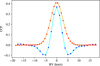 |
Fig. 1 Time-averaged CCFs (templates) of ϵ Eri (red) and TZ Ari (blue) with the corresponding Gaussian model fit for ϵ Eri (orange) and the two-component Gaussian model fit for TZ Ari (cyan). |
2.3 Basic data analysis
To identify periodicities in the time series, we employ the Generalised Lomb–Scargle (GLS, Zechmeister & Kürster 2009) periodogram. The significance of the detected peaks is assessed using false-alarm probability (FAP) levels derived via bootstrap resampling (Efron & Tibshirani 1985). We classify signals as tentative or significant if their power exceeds the 1% or 0.1% FAP levels, respectively.
We present the RV and activity indicator time series together with their GLS periodograms for ϵ Eri in Fig. 2. All time series exhibit significant power at the stellar rotation period and its first harmonic, both highlighted in purple. Similarly, Fig. 3 shows the corresponding data for TZ Ari. In this case, the RV, CON, and BIS time series display significant variability at the stellar rotation period as well as at its daily alias (1 − 1/1.96 = 1/2.04 d−1). In addition, we observe long-term variability in the RVs associated with the orbital motion of TZ Ari b. Since GLS models are sinusoidal, the planet’s eccentricity shifts the highest peak slightly with respect to the literature value (Quirrenbach et al. 2022). The CON time series exhibits a downwards trend, introducing excess power at low frequencies in the periodogram, while the FWHM shows a significant signal at 40.17 d.
In Appendix B, we list the significant periods and amplitudes retrieved via a pre-whitening procedure. This process involves iteratively identifying the most significant periodogram peak, fitting the RVs with a sinusoidal function of the same frequency as that peak, and subtracting it from the time series until no power crossing the 10% FAP threshold remains.
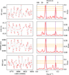 |
Fig. 2 Time series (left) and GLS periodograms (right) of the RV and activity indicators derived from the CCFs for ϵ Eri. We mark in purple the stellar rotation period (11.2 d) and its first harmonic (5.6 d). The 0.1, 1, and 10% FAP levels are shown with dashed orange lines. |
2.4 Synthetic data
2.4.1 StarSim modelling
We generated synthetic time series data using the StarSim1 code (Herrero et al. 2016; Rosich et al. 2020; Gomes et al., in prep.) in order to model the test stars. StarSim is a physically motivated stellar activity simulator that produces synthetic photometric and spectroscopic observables by modelling the inhomogeneous surface of a rotating star. The stellar disk is discretised into surface elements corresponding to three distinct components: quiet photosphere, cool spots, and bright faculae. Each component is represented using a high-resolution synthetic spectrum from the PHOENIX library (Husser et al. 2013), selected to match the appropriate temperature, surface gravity, and metallicity. The library also includes spectra computed at different limb angles to account for centre-to-limb variations across the stellar disk. Rather than synthesising full high-resolution spectra from the surface maps, the simulator computes the CCF corresponding to each surface element directly, resulting in a considerable reduction of the computing time. This CCF computation process explicitly emulates the raccoon pipeline, employing the identical masks and velocity sampling steps applied to the observational data.
We constructed tailored stellar models for each target star using constraints on stellar parameters from the literature (see Table 1). To estimate the contrast temperature difference between photosphere and spot and the convective blueshift, we adopted the empirical relations from Herbst et al. (2021) and Liebing et al. (2021). However, we allowed for wide uniform priors on these parameters rather than fixing them to a single best-fit value. This ensured that the relationships do not impose overly strong constraints on the simulated values, providing the NN with a diverse training set required to generalise well.
We also simulated a large ensemble of stellar surface maps with active regions randomly distributed across the visible disk. Each active region is modelled as a circular spot, characterised by seven parameters: (1) appearance time, (2) lifetime, (3) colatitude, (4) longitude, (5) spot radius, (6) linear growth rate, and (7) linear decay rate. Surrounding each spot is a facular region, modelled as a concentric ring. The facular area is parametrized using a global facula-to-spot area ratio, Q, which is fixed for each simulation. As shown in previous studies (Lanza et al. 2003; Silva-Valio et al. 2010; Dumusque et al. 2014; Herrero et al. 2016), modelling circular spots surrounded by a facular corona successfully reproduces spot maps for high precision photometry of the Sun and other stars.
However, several studies combining Solar Dynamics Observatory (SDO) images and magnetograms of the Sun with RVs have demonstrated that the Sun is facula-dominated, possessing an extensive network of standalone faculae that persists even during solar minimum when spots are absent (Collier Cameron et al. 2021; Haywood et al. 2022). Consequently, an independent treatment of spots and faculae is typically preferred to accurately simulate such networks (Zhao et al. 2025). Given the high activity levels of our specific test targets (Sect. 2) and our objective to restrict the dimensionality of the parameter space, we keep the Q-factor approximation for this study. We note that this simplification is no longer present in the upcoming solar-benchmarked branch of the StarSim code (SunSim, Stucki et al., in prep.).
For simplicity, we assumed that each active region maintains a constant maximum size over most of its lifetime, with linear growth and decay timescales lasting a few days. Although more complex evolution laws for active regions could be implemented, the large number of simultaneously evolving regions, each with different lifetimes, locations, and appearance times, effectively captures the stochastic nature of surface inhomogeneities and approximates the effects of more realistic evolution scenarios.
We calibrate the simulations by adjusting the parameters of the active regions – specifically their number and size distributions – in order to reproduce the typical observed amplitudes and scatter in the spectroscopic time series. It is important to note that our objective was not to recreate the exact epoch-by-epoch RV pattern of the observations, nor did we perform a simultaneous fit (e.g. via Markov chain Monte Carlo, MCMC) of the spot contrast, convective blueshift, and active region geometries to the exact time series. Instead, our goal is to generate a robust training dataset that statistically matches the macroscopic properties of the observed stellar jitter, such as the overall root-mean-square (RMS) scatter, typical periodogram amplitudes, and the amplitude ratios between different CCF indicators. By maintaining a wide range for these parameters, we ensure the simulations retain sufficient generality to account for unexplained variability in the observed RV data, such as instrumental noise or unknown planetary signals. In Sect. 7.5, we discuss the current shortcomings of our simulations in matching some of these statistical metrics.
We simulated between 15 and 25 active regions for ϵ Eri, while we used between 80 and 110 for TZ Ari. This number is significantly larger in the latter case due to its longer observational time baseline of over 1400 d. Spot radii are drawn from a uniform distribution in the range of 3–6° for ϵ Eri and 6–8° for TZ Ari. We also vary the Q parameter, using values between 0 and 9 for ϵ Eri. For TZ Ari, we fix Q = 0 as it is an M5 dwarf, where spot-induced variability dominates (Herrero et al. 2016; Baroch et al. 2020) and faculae have been found to be dark, rather than bright, in 3D magnetohydrodynamic simulations (Johnson et al. 2021; Bhatia et al. 2026).
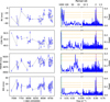 |
Fig. 3 Time series (left) and GLS periodograms (right) of the RV and activity indicators derived from the CCF for TZ Ari. The stellar rotation period (1.96 d) is marked in purple; the planetary orbital period from the literature (722.05 d; Quirrenbach et al. 2022) is marked in light blue; and the 0.1%, 1%, and 10% FAP levels are shown with dashed orange lines. The frequency axis of the periodogram show two scales split at 0.035 d−1 to better visualise long-term variability. The RVs display low-frequency signals associated with the Keplerian motion of TZ Ari b, while the CON and FWHM show lower-frequency stellar activity signals. |
2.4.2 Noise injection
In addition to modelling stellar activity using StarSim, we simulate the impact of photon noise on the CCF. To ensure our synthetic observations are realistic, we inject noise patterns that match the statistical characteristics of the actual observations. We quantify the noise budget for each target star by computing the ratio of the mean observational error of each spectroscopic data to the total root-mean-square (RMS) of its observed time series (Sect. 3.4). This allows us to estimate the fractional contribution of noise to each time series and injects Gaussian noise according to this ratio. A summary of the estimated noise levels for each time series is provided in Appendix B.
3 Theoretical framework
When not considering the influence from instrumental effects, we assume that a spectroscopic observation O(v, t) in the exo-planet domain (e.g. spectrum, single line, CCF), depending on the vector of RV v, and the time of observation t, can be influenced by the following two effects: (1) an orbiting planetary companion that induces a non-chromatic Doppler shift in v, and which we denote in the following with ϵ, and (2) by stellar activity, which induces distortions on the spectral line shapes, including apparent line shifts, and which we denote in the following with κ.
We can decompose any spectroscopic observation, O(v, t), as
 (1)
(1)
where Bn(v) is a set of functions, hereafter basis functions, parametrized by time-dependent coefficients an(t). The term E(v, t) represents the residual uncertainty of the decomposition, and N is the number of decomposition terms, where N ≤ Nv. Nv refers to the number of elements at which u is evaluated. Strictly speaking, no information is lost if N = Nv. However, our aim is to condense the original observation into a smaller number of components with minimal loss of physical information. In the following, we explain how to isolate an orthonormal component from Bn(v), which contains only information on the velocity shifts, from other components only containing information on the shape distortions.
3.1 Isolating the line shift component
If we separate the contribution from Doppler shifts (Oϵ) from the effects of stellar activity (O∗)2, we can write
 (2)
(2)
where I(v) is a function of ones and c0(t) is a constant. In the case where the observation is only affected by ϵ, this induces a shift:
 (3)
(3)
Therefore, we can apply the Taylor expansion of Oϵ with respect to ϵ around v:
 (4)
(4)
where Or(v) is the undistorted rest frame, and  . In practical applications, this theoretical undistorted rest frame is approximated by our empirically derived time-averaged template CCF, T(v), as discussed in Sect. 4.1. Second-order expansion terms 𝒪(ϵ2) are negligible for the case of small ϵ, typical of planetary companions.
On the other hand, the stellar activity changes in v can be written in the most general way as
 (5)
(5)
Here, s(t) is a vector with an unknown number of components describing pure line shape distortions. Since we do not know the functional dependence of these components on physical parameters, a multivariate Taylor expansion is not feasible. The only constraints we imposed on s(t) is that they are orthogonal to the line shift component, ensuring that κ(t) captures the net line shift. In the most general way, we can then decompose the stellar activity part O∗(v, t) of the observation with a Taylor expansion with respect to κ and capture the pure line shape distortions with Gn(v), hereafter the distortion basis function:
 (6)
(6)
where gn(t) are the time-dependent coefficients describing Gn(v). If we combine Eqs. (2)–(6), we can write
 (7)
(7)
where l(t) includes both the Doppler shift and the shift induced by the distorted line, i.e. l(t) = ϵ(t) + κ(t), and c1(t) is a scaling factor that multiplies the undistorted rest frame Or(v), which in this case is equal to 13.
We thereby decomposed our observation O(v, t) into a basis function B that contains a line-shifted component captured by  and a distortion basis function, G(u). Comparing the above with Eq. (1), we found
![Mathematical equation: $B(v) = [I(v),{O_r}(v),O_r^\prime (v),{G_2}(v), \ldots ,{G_{N - 1}}(v)],$](/articles/aa/full_html/2026/06/aa59683-26/aa59683-26-eq18.png) (8)
(8)
![Mathematical equation: $a(t) = [{c_0}(t),{c_1}(t),l(t),{g_2}(t), \ldots ,{g_{N - 1}}(t)].$](/articles/aa/full_html/2026/06/aa59683-26/aa59683-26-eq19.png) (9)
(9)
We note, that ϵ and κ cannot be determined independently and are mathematically degenerate. This degeneracy can only be broken by relating the physical or statistical properties of the c0, c1 and gn coefficients to κ (see Sect. 5).
3.2 Distortion basis functions
For the general framework many different choices for the distortion basis functions Gn(v) can be used. PCA isolates the principal modes of variability of O(v, t). But this method does not distinguish between the different sources of variability (Doppler, activity and instrumental) nor does it ensure the orthogonality of its components to  . PCA was applied in Doppler-free observations on an orthogonalised O(v, t) with respect to
  in Klein et al. (2024), and on the autocorrelation function of O(v, t), in Collier Cameron et al. (2021). An alternative option would be to use the Fourier basis, as proposed in Zhao & Tinney (2020). The basis consists of sine and cosine functions of different frequencies that are orthogonal to each other. However, since the basis is periodic overall v, it puts equal weight on the central part of the CCF and in the wings, which are heavily affected by noise.
For a Gaussian-like observation O(v, t), such as a CCF or a specific spectral line, we propose using the Hermite basis as the distortion basis function, which is defined as
 (10)
(10)
where x = (v − v0)/σ is the normalised velocity coordinate centred at v0, scaled by the width σ, and Hn(x) are the Hermite polynomials. These are defined by the recurrence relation
 (11)
(11)
where H0(x) = 1 and H1(x) = 2x.
A Hermite basis can be understood as a weighted generalisation of the monomial basis xn, which is used to compute the central moments of a function. However, using pure monomials as basis functions leads to their divergence at large |x|. By introducing a Gaussian weight function to the monomial basis function, the Hermite basis effectively suppresses these divergences and delivers an estimate of the orthonormal central moments of a Gaussian-like function O(v, t). Crucially, a Gaussian multiplied by Hermite polynomials forms a basis that is mathematically orthogonal and complete. This completeness is a primary motivation for our choice, as it guarantees that any smooth deviation or asymmetry in the line profile can be accurately represented.
In principle, the distortion basis functions can be constructed using the n-th order derivatives of the Gaussian fit to the observation O(v), with n > 2, given that the G0(x) and G1(x) components are already accounted for in our general basis function B(v) by the Or(v) and  components (Eq. (8)). For non-Gaussian profiles, such as M dwarfs similar to TZ Ari (Fig. 1), we apply a multi-Hermite basis. We model the reference Or(v) by fitting a sum of two Gaussians, prioritising the simplest solution with the fewest free parameters. In the case of TZ Ari, the optimal fit combines a narrow positive Gaussian for the core with a broad negative Gaussian for the wings (Fig. 1).
3.3 Calculation of coefficients
We determined the optimal coefficients an through a χ2 minimisation process:
 (12)
(12)
This process can be rewritten as
 (13)
(13)
If we orthonormalise Bn, so  , this simplifies to
 (14)
(14)
The coefficients that minimise χ2 are then obtained by solving
 (15)
(15)
and hence can be directly determined from the basis function Bn and the observation O(t). The different an(t) coefficients are independent from each other if B(v) is orthogonal. As explained in Sect. 3.2, the Hermite basis is an orthogonal basis, but it may not be orthogonal to the other components of the basis B(v), namely I(v), Or(v), or  .
.
The orthogonality of B(v) can be achieved using the algebraic Gram-Schmidt process, which transforms any set of linearly independent functions into an orthogonal set. Given a non-orthogonal function FN, we orthogonalised it with respect to Bn using the iterative procedure
 (16)
(16)
 (17)
(17)
where fN is the intermediate unnormalised function and ∥ · ∥ denotes its norm.
3.4 Coefficient errors
The uncertainties in the coefficients are obtained by propagating the errors from two independent sources: (1) the flux uncertainties of the observations, and (2) the uncertainties in the single-or multi-Gaussian fit to the template, from which the distortion basis functions are constructed. The total uncertainty in each coefficient can therefore be expressed as
![Mathematical equation: $\delta {a_n}(t) = \sqrt {\mathop \sum \limits_{i = 1}^{{N_v}} [{B_n}{{({v_{i)}}\delta O({v_{i,}}t)]}^2} + [O({v_{i,}}t)\delta {B_n}{{({v_{i)}}]}^2}} .$](/articles/aa/full_html/2026/06/aa59683-26/aa59683-26-eq33.png) (18)
(18)
The uncertainty in the observed profile O(v, t) includes both photon noise and read-out noise (Appendix C), as described in Lafarga et al. (2020). To compute realistic noise estimates per pixel, O(v, t) must be sampled at the physical pixel size of the detector. However, the Gram-Schmidt orthonormalisation used to construct the basis functions Bn makes an analytical expression for δBn intractable. Instead, we propagated the uncertainties from the Gaussian-fit parameters into the orthonormalised basis by computing the formal covariance from the fit and propagating it through the coefficient definition
 (19)
(19)
where Jn is the Jacobian vector of partial derivatives of the coefficient an(t) with respect to the set of fitted parameters p, and Σp is the full covariance matrix of the fit. The Jacobian is defined as
![Mathematical equation: ${J_n} = {{\partial {a_n}(t)} \over {\partial p}} = \left[ {{{\partial {a_n}(t)} \over {\partial {p_1}}},{{\partial {a_n}(t)} \over {\partial {p_2}}}, \ldots ,{{\partial {a_n}(t)} \over {\partial {p_k}}}} \right],$](/articles/aa/full_html/2026/06/aa59683-26/aa59683-26-eq35.png) (20)
(20)
where k is the number of fit parameters. Since these derivatives are not analytically tractable, we estimated them numerically using finite differences. For each parameter pk, we computed
 (21)
(21)
where ∆ is a small perturbation to the parameter pk.
3.5 Explained variance ratio
To evaluate the contribution of each coefficient an to the reconstruction of the original time series, we compute the explained variance ratio (EVR), a metric analogous to that used in PCA. The EVR quantifies the fraction of the total variability in the full time series of O(v, t) captured by a given time series coefficient:
![Mathematical equation: $EV{R_n} = {{\mathop \sum \nolimits_{j = 0}^{{N_T}} {a_n}{{(t)}^2}} \over {1/{N_v}\mathop \sum \nolimits_{i = 1}^{{N_v}} \mathop \sum \nolimits_{j = 0}^{{N_T}} {{\left[ {w({v_{i)}}\left( {O({v_i},{t_j}) - {{\left\langle {O({v_i})} \right\rangle }_t}} \right)} \right]}^2}}},$](/articles/aa/full_html/2026/06/aa59683-26/aa59683-26-eq37.png) (22)
(22)
where, in the most general case, a weight function w can be used for the observations. Further, ⟨⟩t is the expected value over t, and NT is the number of observations.
4 Application of the method
Several considerations must be taken into account when applying the theoretical framework to real observational data. The observations shall be flux normalised before applying this framework using, for example, AFS (Xu et al. 2019), rassine (Cretignier et al. 2020), or raccoon (Lafarga et al. 2020). If the continuum is not properly corrected to match the baseline flux level of Or(v), this propagates to the computation of all an(t), given that this continuum level is a multiplicative factor in Eq. (1). Moreover, real observational data are affected by noise, which can bias the estimate of the EVR. We adopt the Gaussian fit to Or(v) as a weight function, so we can properly weigh down the wings of the CCF, which are predominantly dominated by noise.
4.1 Template construction
As seen in Eq. (7), the decomposition is performed with respect to Or(v), which represents the observation in an undistorted reference frame. This reference is also used to compute its first derivative,  , in order to measure the line shift l(t). In general, however, we do not have access to an undistorted reference observation Or(v). We therefore decomposed our observations with respect to a template T(v) that is constructed by averaging all observations of the time series, t, as explained in Sect. 2.2. We aim to reduce the influence of time-variable distortions and obtain a more stable representation of the stellar signal. The template provides a valid approximation to the undistorted reference profile required for the decomposition. Given that we use a template, generally, c1 ≠ 0, and it will estimate the changes in amplitude.
Consequently, we approximated  by the first derivative of the template T(v). We note that T′(v) was calculated from the first derivative of a cubic spline on T(v). The first element of the Gram–Schmidt process is T′(v), so we could ensure that all other elements of our basis function are orthogonal to line shifts.
4.2 ϵ Eri
As can be seen in the left panel of Fig. 1, the template of ϵ Eri is in good agreement with a single Gaussian profile. We therefore adopted a single Hermite basis for its decomposition. In Fig. 4 the first six components of the decomposition of the ϵ Eri CCFs are shown in red, including the Hermite basis from G2 to G4. In Fig. 5, we show in red the individual and cumulative EVR per component. The individual EVR peaks at the c1 component, connected to the template T, and decreases monotonously as we go to higher order distortion coefficients. The first five coefficients explain 91.7% of the variance, while 11 components account for 97.8%. Notably, our method enables the quantification of the contribution to the variance by line shifts via the l coefficient, which alone accounts for 19.3% of the total variance.
In Fig. 6, we show (i) the reconstruction of the differential (template-subtracted) CCFs at six random epochs by adding the contribution from the different basis function components (left column), (ii) the time series of the first eight coefficients (middle column), and (iii) their corresponding GLS periodograms, (right column). Coefficients up to g6 trace the stellar rotation period, marked with purple lines, with l, g2 and g3 also showing sensitivity to the first harmonic at ∼5.6 d. The slight shifts in the exact periodogram peaks across different coefficient orders can be physically attributed to stellar differential rotation (as reported in Croll et al. 2006) and active region evolution. We also note that the baseline offset term, c0, also exhibits sensitivity to stellar rotation. While mathematically defined as a constant, c0 naturally absorbs changes in the overall integrated area of the CCF, whether caused by imperfect flux normalisation or, as in this case, stellar activity driving variations in both the continuum level and line amplitude.
As expected from their lower EVRs, higher-order coefficients contribute less to the signal reconstruction and are increasingly affected by noise, therefore reducing their sensitivity to rotationally modulated stellar activity. For a summary of the general statistics of the distortion coefficients and the identified signals from a pre-whitening process we refer to Appendix B.
Figure D.1 shows the correlation between decomposition coefficients and classical CCF indicators. The strongest correlations are CON with c1, RV with l, FWHM with g2, and BIS with g3, confirming that the decomposition recovers the classical CCF activity indicators. The strongest correlation between decomposition coefficients is between l and g3, and between c1 and g2. Beyond this, higher-order coefficients extend the sensitivity to distortions not captured by classical CCF activity indicators.
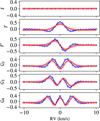 |
Fig. 4 First six basis components for ϵ Eri (Hermite, red) and TZ Ari (multi-Hermite, blue). |
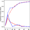 |
Fig. 5 Explained variance ratio (solid) and cumulative variance (dashed) per component for ϵ Eri (Hermite, red) and TZ Ari (multi-Hermite, blue). |
4.3 TZ Ari
Figure 1 shows the template used to compute the basis functions. It displays the characteristic shape of cool M dwarfs (Lafarga et al. 2020). As a result, a double Hermite basis is used to fit this template, consisting of a narrow positive-amplitude Gaussian for the core and a broader negative-amplitude Gaussian for the wings. In Fig. 4, the first six components of the decomposition of the TZ Ari CCFs are depicted in blue, showing a distinct shape for the multi-Hermite case. Figure 5 illustrates the EVRs for the multi-Hermite decomposition coefficients applied to TZ Ari. The EVR peaks at the c1 coefficient, explaining 47.1% of the EVR. The l coefficient alone accounts for 19.6% of the total variance. The g2 coefficient contributes only marginally, while g5 provides a comparatively large contribution to the variance. The cumulative EVR reaches 86.8% at this coefficient, reaching the 97.1% mark if we extend it up to the g9 coefficient.
Figure 7 shows the differential CCF reconstructions (left), coefficient time series (middle), and their corresponding GLS periodograms (right). The stellar rotation period (1.96 d) and its daily alias are clearly recovered in the low-order coefficients; c1, l, g2 and g3. Long-period signals are also observed in c1, l, g2, and g4 (Appendix B). The exoplanetary signal at 772.05 d is significantly detected in the GLS periodogram of l only, as expected.
Figure D.2 displays correlations between decomposition coefficients and classical CCF activity indicators. As for the case of ϵ Eri, the strongest correlations are found between CON and c1, RV and l, FWHM and g2, and BIS and g3. However, the correlations between FWHM and g2, and between BIS and g3 are not as strong as in the ϵ Eri case. The strongest correlation between decomposition coefficients is between c0 and c1, and between l and g3.
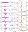 |
Fig. 6 Cross-correlation function decomposition of ϵ Eri with a Hermite basis. Left: contribution of consecutive basis components to the differential CCF reconstruction. We displayed six illustrative epochs randomly selected to visualise the temporal variability of the line-shape distortions. The observed differential CCFs are shown in grey, while the reconstructed components are colour-coded according to the observation time. Middle: time series of the corresponding coefficients. Right: GLS periodograms of the coefficients. The 0.1%, 1%, and 10% FAP levels are indicated in orange, and the stellar rotation period and its first harmonic are marked in purple. |
5 Neural networks for stellar activity correction
In this section we introduce the NN framework. The goal is to predict and remove the activity-induced RV shifts using the information from the line-shape distortion coefficients.
5.1 Architectures
We have developed a deep-learning model that we refer to as Convolutional-Attention Network for STellar Activity Removal (CANSTAR). An overview of the CANSTAR architecture is provided in Fig. 8. Several (Nc) convolutional layers apply Nf localised filters to the input time series, which consist of the amplitude coefficient c1(t) and the distortion coefficients gi(t). We explicitly exclude the baseline offset term, c0(t), from the inputs because it is highly susceptible to flux normalisation issues and sensitive to noise sources not accounted for in our simulations. These filters extract short-term, high-frequency features in the input according to the filter size Ns. The convolutions are applied with appropriate padding and stride, ensuring that the output feature maps keep the same temporal dimension as the input. Each convolutional layer uses multiple filters, producing a set of feature maps that capture different local attributes of the data.
Following the convolutional layers, the extracted feature maps are passed into Nte transformer encoder layers. These layers consist of a multi-headed self-attention mechanism followed by a position-wise feed-forward network, as defined in Vaswani et al. (2017). The self-attention mechanism captures dependencies across the full temporal domain, allowing the network to model both short- and long-term correlations in the data. The embedding dimension of the attention layer is matched to the number of convolutional filters, and Nh attention heads are used to extract different temporal features. Finally, the output of the transformer block is flattened and passed through a linear projection layer, producing the predicted κ(t) time series. This hybrid architecture follows principles similar to those proposed by Liu et al. (2020) and Guo et al. (2022), who demonstrated the effectiveness of combining convolution and attention in the analysis of time series and image data.
We also tested a simpler fully connected network (FCN). This architecture processes only instantaneous snapshots of the line-shape distortion coefficients, gi, without explicitly modelling their temporal evolution. The FCN architecture consists of a sequence Nff of feed forward layers. All input coefficients from a single observation are concatenated into a one-dimensional feature vector, which is fed into the network. The outputs of each layer are fully connected to the inputs of the next by Nn number of neurons. The final layer of the FCN is a linear layer which predicts the final κ.
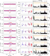 |
Fig. 7 Same as Fig. 6 but for the multi-Hermite basis applied to TZ Ari. We also mark in light blue the planetary orbital period from the literature (722.05 d; Quirrenbach et al. 2022). |
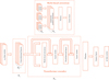 |
Fig. 8 Schematic representation of CANSTAR (bottom), a convolutional attention network designed to predict the stellar activity contribution to line shifts, κ(t), from the time series of distortion coefficients, gi(t). The input coefficients are treated as independent channels and processed through a series of one-dimensional convolutional layers that extract local temporal features. The convolutional outputs are then passed to a transformer encoder module, which consists of a multi-head self-attention part (top) with different ‘heads’, where each one of them focuses on different temporal dependencies within the data, and their outputs are combined, normalised, and propagated through additional attention layers. Finally, the resulting features are flattened and projected through a linear layer to produce the predicted κ(t) time series. |
5.2 Neural network training
Training is performed using synthetic datasets generated with the StarSim code (Sect. 2.4.1). For each target star, we generate a dataset of 500 000 time series simulations. The dataset is divided into training (80%), validation (10%), and test (10%) sets. The training set is used to find the optimal parameters of the NN based on the minimisation of the Mean Squared Error (MSE) between the true labels, i.e. the κ(t) component of l(t), and the prediction by the network. We apply z-score normalisation to the input and output dataset, meaning we subtract the mean value of each simulated dataset and rescale them according to the standard deviation of the full dataset.
We optimised all network architectures using the Adam optimiser (Kingma 2014) implemented in PyTorch (Paszke et al. 2019). We selected as the final model the model just before the improvement in validation MSE plateaus while the training MSE continues to decrease significantly, ensuring we avoid the over-fitting regime. We reserved this test set for the evaluation of the performance of this final network on unseen data. We saved the residual relative error (RRE) from the final model, defined as the ratio of the residual RMS after correction to the original RMS (Perger et al. 2023).
Tested and adopted hyper-parameters for CANSTAR (top) and FCN (bottom).
5.3 Hyper-parameter choices
Each architecture is defined by several hyper-parameters. We performed a systematic hyper-parameter search to determine these values. The tested and final selected configurations are summarised in the upper and lower parts of Table 2 for CANSTAR and the FCN, respectively. The final selection was based on minimising the validation set MSE, prioritising the simplest effective choices.
6 Results
We trained separate CANSTAR models for each target star (ϵ Eri and TZ Ari) for different noise-level regimes (noiseless and similar to the observations; see Sect. 2.4.2) and including different numbers of distortion coefficients. The aim with this training strategy was to evaluate the ability of CANSTAR to mitigate stellar activity as a function of the target star and S/N of the observations. In order to test the capability of modelling stellar activity by the different distortion coefficients, we iteratively trained CANSTAR networks using more coefficients as inputs, following the natural order of the coefficients from the Hermite and multi-Hermite formalism. We repeated this same training strategy for the FCN.
After the training phase, we selected the best-performing network trained on noise similar to the observations, defined as the model that minimises the RRE while requiring a smaller number of distortion coefficients. To quantify the stability of the solution, we trained five independent instances of this architecture. Although the variance in the predictions on the synthetic test set is negligible, it can have an effect when predicting on the real observational data. To account for this, we applied the full ensemble of five networks to the data. Furthermore, to propagate the observational uncertainties, we generated 1000 Monte Carlo realisations of the input distortion coefficients, perturbed according to their measurement errors. Each of the five networks generates predictions for all 1000 realisations. We adopted the median of this combined distribution as the final activity model and used the standard deviation as the total uncertainty.
6.1 Simulated data
We show the performance on the simulated test set of CANSTAR and FCN in Fig. 9. In the noiseless case, CANSTAR achieves an RRE of 3.7% for ϵ Eri and 3.3% for TZ Ari, when trained with 15 coefficients. Notably, the performance already saturates at 7 coefficients, reaching an RRE 5.9% for ϵ Eri and 3.9% for TZ Ari. By contrast, the FCN achieves an RRE of 12.7% for ϵ Eri and 4.9% for TZ Ari after training with 15 coefficients. CANSTAR outperforms the FCN in RRE reduction, requiring fewer coefficients to reach the same level of activity correction.
With noise matched to the observed RV uncertainties, CANSTAR reaches an RRE of 12.9% for ϵ Eri and 35.7% for TZ Ari, when trained with 15 coefficients. On the other hand, the FCN network reaches an RRE of 38.8% for ϵ Eri and 49.1% for TZ Ari. In both regimes, the RRE reduction plateaus at a smaller number of coefficients than in the noiseless case, highlighting the fact that higher-order coefficients are increasingly dominated by noise and contribute little to the correction.
There is also a difference in the performance of the network between the two target stars. For ϵ Eri, the most significant coefficients when correcting for activity are the c1, g2 and g3 coefficient. In the case of TZ Ari, c1 and g2 are not as correlated to the line shift component as g3, which is the most informative for training both CANSTAR and the FCN network. We also note that we reached a lower overall RRE reduction for the cases of ϵ Eri with observational noise when compared to TZ Ari. This is because the former is a much brighter star with significantly higher S/N observations.
6.2 ϵ Eri
For ϵ Eri, we selected the network trained on the first five distortion coefficients as the best-performing configuration. We applied z-score normalisation to the real observed datasets in order to minimise the discrepancy in the scale between observed and synthetic datasets (Appendix E). We explored the inclusion of a linear scaling parameter to fine-tune the amplitude of the predictions given the loss of the absolute scale due to this. The scaling parameter converged to a value of α = 0.9. This value is close to unity, as expected, given that the RV variability of ϵ Eri is dominated by stellar activity on these timescales. Therefore, the z-score normalisation used during training accurately reflects the scale of the observed activity signal (Appendix E).
CANSTAR’s correction for ϵ Eri is shown in Fig. 10. The predicted RV time series closely matches the observed data, and the GLS periodogram reveals that the model effectively captures the dominant stellar rotation signal and its first harmonic. After subtracting the predicted κ component from the observations, we obtain an RRE of 52.5%, resulting in a final RMS of 2.46 m s−1 (Table 3). The power of signals associated with stellar activity, which peak at 12.53 d and 6.26 d, is significantly diminished, decreasing below the 10% FAP level. No signal remains in the periodogram above the 10% FAP level. The residuals are in agreement with the ϵ Eri b solution presented in Thompson et al. (2025), which just produces a trend for the narrow observing window.
We injected sinusoidal signals directly into the RV time series to quantify the detection limits at different frequency ranges. We injected sinusoidal signals with frequencies ranging from 0.5 to 1/Tbase (where Tbase is the time baseline of the observations), in steps of 1/5Tbase. The semi-amplitude grid spans from 0.5 m s−1 to the RMS of the observations, 4.5 m s−1, in steps of 0.1 m s−1. For each combination of frequency and semi-amplitude, we injected ten evenly spaced phases from 0 to 2π. The phase-averaged results are illustrated in Fig. 11 as heat maps showing the relative difference between the injected and recovered semi-amplitudes (K) and frequencies for the CANSTAR activity-corrected residuals. We defined the detection limit as the minimum injected amplitude required to recover the semi-amplitude with a specific precision (e.g. 10% or 30%), provided the frequency is also retrieved within a 10% relative error. Using this criterion, the detection limits are 2.51 ± 0.43 m s−1 for a 10% precision threshold and 1.99 ± 0.41 m s−1 for a 30% threshold. As expected, the recovery of planetary signals becomes more challenging around the stellar rotation period and its harmonics due to the inherent degeneracy between Keplerian and activity-induced variability. We also show in Appendix F the detection limits for the null hypothesis case. The detection limits are 3.99 ± 0.18 m s−1 (10% precision) and 3.87 ± 0.18 m s−1 (30% precision).
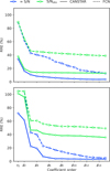 |
Fig. 9 Residual relative error of ϵ Eri (top) and TZ Ari (bottom) StarSim data after correction with CANSTAR (solid line with circle marker) and an FCN (dashed line with square marker) for the noiseless case (blue) and for the case with noise equivalent to the observations (green). |
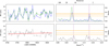 |
Fig. 10 Top: Radial velocity time series (left) and GLS periodogram (right) of the HARPS ϵ Eri data (blue) compared to the stellar activity signal predicted by CANSTAR (green). Bottom: Residuals after subtracting the prediction (grey), with their corresponding periodogram (right). The 10%, 1%, and 0.1% FAP levels are indicated by dashed orange lines and the stellar rotation period (11.2 d), and its first harmonic (5.6 d) is marked in purple. The residuals are compatible with the ϵ Eri b solution (red; Thompson et al. 2025). |
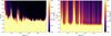 |
Fig. 11 Detection limits in the ϵ Eri residuals after applying CANSTAR’s correction, shown as a function of the difference between injected and retrieved frequencies (left) and semi-amplitudes (right) for the different injected frequencies and semi-amplitudes sinusoidal signals. |
6.3 TZ Ari
For TZ Ari, we similarly select the network trained on the first three order coefficients as the best-performing configuration. Unlike ϵ Eri, the RV variability of TZ Ari is dominated by the high-amplitude Keplerian signal of the planet (K = 21.11 m s−1; Quirrenbach et al. 2022). Consequently, we need to perform a joint fit for the Keplerian solution of the planet together with the CANSTAR activity correction. We use the MCMC sampler emcee (Foreman-Mackey et al. 2013), simultaneously solving for the orbital parameters of TZ Ari b and the optimal value of the scaling parameter of the CANSTAR activity correction, α. For the MCMC parameter optimisation, we employed 700 walkers, each run for 32 000 steps to ensure convergence of the chains. The first 2000 steps were discarded as burn-in. The adopted priors and the resulting optimised parameter values are listed in Table 4, together with the Kep-lerian solution we retrieve if we do not apply the CANSTAR activity correction. We also compare these results to a GP framework using a simple harmonic oscillator (SHO) kernel, reproducing the strategy of Quirrenbach et al. (2022) but restricting their multi-instrument dataset to CARMENES only (Appendix G).
We compare in Fig. 12 the posterior distribution of the common parameters between the CANSTAR and GP model. CANSTAR activity correction allows for a better determination of the period and semi-amplitude of the planet, compared to the GP modelling. The GP solution outperforms CANSTAR in reducing the RV scatter, as illustrated by its lower fitted jitter term, which captures additional noise sources not captured by the model. This is expected given the strong flexibility of GPs at filtering white noise and being prone to overfitting (Blunt et al. 2023). The posterior distributions of the CANSTAR + Keplerian model parameters are shown as corner plots in Appendix H.
Figure 13 presents the time series and GLS periodograms of the CARMENES RV observations (blue), together with the CANSTAR activity correction (green), the Keplerian solution (red), and the residuals (grey). In the time series plot (left), the green curve represents the sum of the CANSTAR correction and the Keplerian orbit. This allowed us to visualise the total fit to the observations. The resulting model successfully captures both the Doppler and stellar activity signals present in the data. Notably, the planetary origin of the long-period signal is confirmed by the periodogram (right panel), where the CANSTAR model (green) is shown in isolation and is clearly insensitive to the planetary signal. After applying the correction, the RV residuals show an RRE of 62.4%, measuring the ratio with respect to the variability after subtracting the fitted Keplerian model (Table 3). The residual GLS periodogram of the CANSTAR correction is largely flat, showing only a minor insignificant peak at 64.7 d (FAP = 11.7%). In contrast, the residuals of the GP + Keplerian model (Fig. 14) display two distinct signals above the 1% FAP level at 37.2 d and 41.4 d. These periodicities correspond to yearly aliases of one another (1/37.2 ≈ 1/41.4 + 1/365) and are likely caused by uncorrected stellar activity, given the significant variability observed in the FWHM and g2 indicators at 40.18 d (Figs. 3 and 7).
During the final CARMENES observing season, when the star was monitored more intensively, the temporal sampling becomes sufficient to mitigate rotationally modulated stellar activity more effectively with CANSTAR. A zoom-in of this last season is shown in Fig. 13, where the RRE is further reduced to 33.4%.
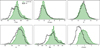 |
Fig. 12 Histograms showing the posterior distribution of the shared parameters between the CANSTAR and GP correction methods used to model the TZ Ari RV data. |
Radial velocity statistics before and after CANSTAR correction.
7 Discussion
7.1 The value of orthogonal decomposition
Standard activity indicators derived from the CCF rely on a simple Gaussian fit. This approach is suboptimal for capturing complex line deformations, requiring ad hoc diagnostics such as the BIS to quantify asymmetries. Furthermore, as shown in Fig. 1, the Gaussian model fails to accurately reproduce the non-Gaussian, double-humped CCFs characteristic of many M dwarfs.
A key advantage of the theoretical framework presented here is its generality, allowing for the construction of basis functions tailored to the specific spectral type of the star. We demonstrate that the standard Hermite basis is optimal for describing Gaussian-like CCFs, while M dwarf CCFs exhibiting pronounced double humps are better modelled by the multi-Hermite basis. For the specific case of TZ Ari, the humps are largely symmetric, making a two-Gaussian fit sufficient to construct G0. However, more complex or asymmetric CCF morphologies might necessitate three or more Gaussians. A robust and automated approach to determine the optimal number of Gaussians for the mother function is to perform a systematic model selection – for instance, by minimising the Bayesian Information Criterion (BIC) – when fitting the time-averaged template CCF.
This theoretical framework enables the recovery of the classical CCF activity indicators, as seen in the high level of correlation between c1-CON, g2-FWHM and g3-BIS (Sects. 4.2 and 4.3), in addition to extending the analysis to higher order variability. Moreover, the EVR allowed us to quantify the actual number of distortion basis components needed to describe the observed CCFs.
While a mathematical degeneracy remains between true Doppler shifts induced by planets (ϵ) and apparent shifts caused by stellar activity (κ), the orthogonal decomposition ensures that our inputs to the NN, the coefficients gn(t), capture shape information that is mathematically independent of the target variable l(t). Using the first three distortions coefficients, (c1, g2 and g3), we are effectively using similar information to the classical CCF activity indicators, but extending the analysis to higher order coefficients allowed us to improve the activity mitigation performance.
More generally, the distortion coefficients are not limited to the specific architecture proposed. They could serve as inputs for other stellar mitigation techniques, such as the multi-dimensional GP framework. Finally, this parametrisation is computationally efficient and agnostic to the specific pipeline used. It can be easily implemented in standard reduction codes such as raccoon or the ESO DRS.
Comparison of orbital parameters for TZ Ari b.
7.2 Temporal awareness in activity correction
The comparison between CANSTAR and the FCN highlights the critical role of temporal information. As shown in Fig. 9, the FCN, which treats observations as independent snapshots, fails to reach the same correction performance as CANSTAR, particularly in noisy regimes.
Stellar activity is inherently a time-correlated process. Active regions evolve, migrate, and reappear over the stellar rotation period. The inclusion of self-attention mechanisms allows CANSTAR to ‘learn’ these temporal correlations, effectively using the past and future context of the distortion coefficients to mitigate stellar activity occurring at different timescales. This capability is illustrated by the fact that CANSTAR effectively saturates its performance with fewer input coefficients than the FCN. By including the temporal context, the network can extract more information from the lower-order coefficients (c1, g2, g3), reducing the reliance on higher-order terms that are more affected by photon noise.
For exoplanet host stars with sparse RV monitoring, temporal correlations may be lost. In such cases, activity mitigation strategies that do not rely on temporal continuity remain necessary. Our results with the FCN demonstrate the advantage of using the full set of distortion coefficients as inputs compared to classical CCF activity indicators, which are equivalent to using only the lower-order terms (c1, g2, g3).
7.3 Noise estimation in neural network predictions
We emphasise the critical importance of correctly propagating photon noise from the spectral level to the CCF and subsequently to the derived activity indicators (see Sect. 3.4 and Appendix C). These precise noise estimates allowed us to inject realistic noise into the synthetic dataset (Sect. 2.4.2). Training on data with realistic noise properties is essential to prevent the network from over-fitting to specific noise patterns. Furthermore, these estimates enable us to quantify the uncertainty of the NN predictions. As detailed in Sect. 6, we achieve this by evaluating the network on noisy realisations of the input data (propagating measurement error) and by training an ensemble of independent networks to estimate the model variance.
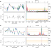 |
Fig. 13 Radial velocity time series and GLS periodograms for TZ Ari showing (a) the complete multi-season dataset and (b) a detailed view of the final observing season. For each panel, the top row displays the CARMENES data (blue), the CANSTAR prediction (green), and the Keplerian solution (red). In the time series, the green curve includes the Keplerian signal to illustrate the full fit, whereas in the periodogram it represents the activity model alone. The bottom row shows the residuals after subtracting both the CANSTAR activity correction and the Keplerian model (grey). The 10%, 1%, and 0.1% FAP levels are indicated by dashed orange lines. The stellar rotation period (1.96 d) is marked with a purple dashed line, and the newly derived planetary orbital period (789.92 d) is marked in light blue (not shown in panel (b) due to its shorter time baseline). |
7.4 Comparison with previous studies
This study builds upon the previous work developed in Perger et al. (2023). We have explored different input data, transitioning from classical CCF activity indicators (CON, FWHM and BIS) to time series of distortion coefficients, and different NN architectures, from a CNN to a convolutional attention network. Both studies relied on StarSim data for training. However, in this work, we utilised a newer version of the code that has been improved, both in its physical model as well as on the practical implementation (Gomes et al., in prep.).
We can directly compare the performance of Perger et al. (2023) against CANSTAR regarding stellar activity correction on the ϵ Eri dataset (Fig. 15). The CANSTAR correction matches the observed data better, resulting in an RRE reduction to 52.5% of the original variability, compared to the 67% reduction level of the Perger et al. (2023) results4. The residuals from both approaches show significant differences. The GLS periodogram of the CANSTAR residuals shows a clear mitigation of the rotational period (FAP > 10%). On the other hand, the peak at the rotation period remains highly significant (FAP < 0.1%) in the GLS periodogram of the Perger et al. (2023) residuals. The residuals from both methods display a low degree of correlation, with a Pearson correlation coefficient of 0.38.
In Sect. 6.3, we compared the CANSTAR activity correction on TZ Ari against the GP framework with the SHO kernel from Quirrenbach et al. (2022), but we limited the analysis to CARMENES. CANSTAR achieves compatible but more precise determinations of the semi-amplitude and period of the Keplerian parameters (Fig. 12). The GP achieves a larger reduction of RRE, as illustrated in the lower fitted jitter term. This is expected due to the flexibility of GP modelling solely on RV data, which can lead to over-fitting leaving small residual amplitudes (Blunt et al. 2023). However, two residual signals in the GLS periodogram remain above the 1% FAP level after the GP solution, with periods 37.2 d and 41.4 d. These periods are likely yearly aliases of a stellar activity signal, as evidenced by significant variability in the g2 and FWHM indicators at 40.18 d (Table B.2). In contrast, CANSTAR effectively removes these signals because its correction is explicitly conditioned on the line-shape distortion coefficients. This demonstrates that CANSTAR provides a physically motivated correction that avoids the over-fitting pitfalls of pure RV modelling.
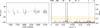 |
Fig. 14 Residual time series (left) and GLS periodogram (right) after subtracting the GP + Keplerian model to the TZ Ari RV data (grey). The 10%, 1%, and 0.1% FAP levels are indicated by dashed orange lines. The stellar rotation period (1.96 d) is shown in purple, the newly derived planetary orbital period (789.92 d) is in light blue, and the two signals exceeding the 1% FAP level (37.2 d and 41.4 d) are marked in black. These likely correspond to stellar activity given the significant (40.18 d) periodicity observed in the FWHM and g2 indicators. |
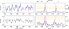 |
Fig. 15 Top: radial velocity time series (left) and GLS periodogram (right) of the HARPS ϵ Eri data (blue) compared to the stellar activity signal predicted by CANSTAR (green) and Perger et al. (2023, magenta). We note that the Perger et al. (2023) did not provide uncertainties to their NN predictions. Bottom: Residuals after subtracting the prediction with their corresponding periodogram (right). The 10%, 1%, and 0.1% FAP levels are indicated by dashed orange lines. |
7.5 Bridging the synthetic gap
We find a difference in performance when evaluating the CANSTAR network on synthetic versus real data. In our noiseless simulations, CANSTAR achieves nearly perfect correction, and even in datasets with injected noise matching the observations, the network achieves an RRE of 12.9% for ϵ Eri and 35.7% for TZ Ari. However, when applied to the real datasets, the RRE becomes 52.5% and 61.6%, respectively. This performance gap indicates that while StarSim provides a physically realistic output, it still lacks certain stellar activity and instrumental effects present in reality.
First, our noise injection procedure currently accounts only for photon noise measured at the spectral level (white noise). However, real observations are affected by instrumental systematics and atmospheric effects that introduce correlated noise into the data. Since our network is trained solely on white noise, it may be less effective at filtering out these complex, non-Gaussian systematic trends. Future synthetic datasets should therefore integrate instrumental systematics to better simulate the red noise floor of the specific spectrograph.
Second, current StarSim simulations rely on 1D PHOENIX stellar spectra (Husser et al. 2013) combined with modified bisector line shapes to simulate the photosphere, spots, and faculae. However, spots and faculae are direct manifestations of the interplay between magnetic fields and the complex 3D structure of the photosphere (Witzke et al. 2022). This dependence on 1D atmospheric models is a shared limitation among current simulators, such as SOAP-GPU (Zhao & Dumusque 2023) and SOAP 4.0 (Cristo et al. 2025).
A significant step towards bridging this physical gap is the use of synthetic spectra derived from 3D magnetohydrodynamic (MHD) simulations. The upcoming version of StarSim (Gomes et al., in prep., Stucki et al., in prep.) is designed to incorporate spectra from the MURaM MPS-ATLAS 3D MHD models (Witzke et al. 2024). By explicitly modelling the 3D structure of the stellar atmosphere driven by convection, this approach will improve the physical prescription of the photosphere, spots and faculae, while enabling the inclusion of other convective phenomena such as granulation and super-granulation. Simulating these phenomena will be essential for extending this framework to less active stars (Reinhold et al. 2019; Meunier & Lagrange 2020).
On the other hand, accurately modelling very active, flaring M dwarfs would require StarSim to simulate coronal heating driven by high-intensity magnetic fields. The self-consistent simulation of stellar chromospheres and flare events remains a significant limitation shared across the entire field (Allen et al. 2026).
8 Conclusions
We have introduced CANSTAR, a novel framework that exploits information on CCF line-shape distortions and their temporal evolution. The framework consists of two main steps: (1) separating pure Doppler shifts from line-shape distortions using an orthonormal basis expansion, which enables the subtraction of distortion coefficients time series, and (2) modelling the temporal evolution of these stellar activity distortions with a convolutional attention network trained on synthetic datasets generated with StarSim.
We have demonstrated that CANSTAR achieves near-perfect stellar activity correction on simulated data, outperforming an FCN that does not explicitly model temporal correlations. The performance worsens when noise resembling that of real observations is injected, primarily because higher-order coefficients become increasingly noise dominated.
When trained on synthetic noisy data and applied to real observations of ϵ Eri and TZ Ari, CANSTAR successfully mitigated a significant fraction of the stellar activity signal. For ϵ Eri, we improved the activity correction provided in Perger et al. (2023) by reducing the RRE from 67% to 52.5%. Applying the CANSTAR correction improves the detection limit for a 10% relative precision in K to 2.51 ± 0.43 m s−1, compared to the baseline of 3.99 ± 0.18 m s−1 obtained for the uncorrected (null hypothesis) case.
For TZ Ari, the network successfully disentangles planetary Doppler shifts from activity-induced signals, yielding improved orbital parameter estimates for TZ Ari b compared to a GP fit. This demonstrates that CANSTAR outperforms the current state-of-the-art solution, enabling both robust activity correction and precise planetary characterisation. After subtracting the Keplerian solution, CANSTAR achieves an RRE of 62.4% on the full dataset. Notably, this residual scatter is further reduced to 33.4% for the final observing season, where the higher cadence allowed for proper sampling of the 1.96 d stellar rotation period.
Beyond the integrated framework, the individual components of CANSTAR offer independent utility. The distortion coefficients obtained from the orthonormal basis expansion can reproduce classical activity indicators while providing sensitivity to additional stellar phenomena via higher-order terms. Furthermore, the convolutional attention network has a general time–aware architecture capable of capturing variability on multiple timescales. Its inputs are not limited to CCF coefficients, but it can be readily adapted to use photometry, chromospheric indices, or line-by-line activity indicators.
Looking forward, there is a clear path to bridge the performance gap between simulations and real data. Future StarSim developments will incorporate spectra from 3D MHD simulations, allowing us to model less active stars where granulation and faculae dominate. By integrating these physical effects along with instrumental systematics into the training sets, we expect to further enhance the network’s predictive power.
Ultimately, this work demonstrates that NNs are not just a future prospect but a present capability, and they already outperform established state-of-the-art solutions, such as GPs, in regimes dominated by complex stellar activity. By effectively using temporal context and high-order line shape distortions, CANSTAR offers a robust pathway to disentangling planetary signals from stellar activity effects. This approach, with further maturation and work closing the gap between synthetic and real data, can be instrumental in pushing detection limits towards the photon-noise floor, which would enable the discovery of lower-mass planets and eventually unlock the domain of exo-Earths.
Acknowledgements
The authors thank the anonymous referee and the editor for their constructive feedback and careful reading of the manuscript. We also warmly thank Pedro Figueira for providing valuable comments that helped improve this work. J.B.-P., M.P., G.A.-E., I.R., J.C.M., O.P. and S.S. acknowledge financial support from Spanish grants PID2021-125627OB-C31 funded by MCIU/AEI/10.13039/501100011033 and by “ERDF A way of making Europe”, PID2024-158486OB-C31 funded by MCIU/AEI, by the programme Unidad de Excelencia María de Maeztu CEX2020-001058-M and by the MaX-CSIC Excellence Award MaX4-SOMMA-ICE, by the Generalitat de Catalunya/CERCA programme, and by the European Research Council (ERC) under the European Union’s Horizon Europe programme (ERC Advanced Grant SPOTLESS; no. 101140786). Views and opinions expressed are however those of the author(s) only and do not necessarily reflect those of the European Union or the European Research Council. Neither the European Union nor the granting authority can be held responsible for them. J.B.-P., M.P. and G.A.-E. also acknowledge financial support from Spanish grant PID2020-120375GB-I00, funded by MCIU/AEI, and Consolidación 2022 CNS2022-136050. J.B.-P. also acknowledges financial support from Spanish grant PRE2022-101942 funded by MICIU/AEI/10.13039/501100011033 and ESF+. M.L acknowledges support by the UKRI (Grant EP/X027562/1). The data production, processing and analysis tools for this paper have been developed, implemented and operated in collaboration with the Port d’Informació Científica (PIC) data center. PIC is maintained through a collaboration agreement between the Institut de Física d’Altes Energies (IFAE) and the Centro de Investigaciones Energéticas, Medioambientales y Tecnológicas (CIEMAT).
References
- Al Moulla, K., Dumusque, X., Cretignier, M., Zhao, Y., & Valenti, J. 2022, A&A, 664, A34 [NASA ADS] [CrossRef] [EDP Sciences] [Google Scholar]
- Allen, N. H., Espinoza, N., Boehm, V., et al. 2026, AJ, 171, 105 [Google Scholar]
- Ambikasaran, S., Foreman-Mackey, D., Greengard, L., Hogg, D. W., & O’Neil, M. 2015, IEEE Trans. Pattern Anal. Mach. Intell., 38, 252 [Google Scholar]
- Anglada-Escudé, G., & Butler, R. P. 2012, ApJS, 200, 15 [Google Scholar]
- Anglada-Escudé, G., Amado, P. J., Barnes, J., et al. 2016, Nat, 536, 437 [Google Scholar]
- Artigau, É., Cadieux, C., Cook, N. J., et al. 2022, AJ, 164, 84 [NASA ADS] [CrossRef] [Google Scholar]
- Baines, E. K., & Armstrong, J. T. 2011, ApJ, 744, 138 [Google Scholar]
- Baranne, A., Queloz, D., Mayor, M., et al. 1996, A&AS, 119, 373 [Google Scholar]
- Baroch, D., Morales, J. C., Ribas, I., et al. 2020, A&A, 641, A69 [EDP Sciences] [Google Scholar]
- Barragán, O., Aigrain, S., Rajpaul, V. M., & Zicher, N. 2022, MNRAS, 509, 866 [Google Scholar]
- Bhatia, T. S., Cameron, R. H., Solanki, S. K., et al. 2026, A&A, 706, A308 [NASA ADS] [CrossRef] [EDP Sciences] [Google Scholar]
- Blunt, S., Carvalho, A., David, T. J., et al. 2023, AJ, 166, 62 [NASA ADS] [CrossRef] [Google Scholar]
- Bouchy, F., Pepe, F., & Queloz, D. 2001, A&A, 374, 733 [NASA ADS] [CrossRef] [EDP Sciences] [Google Scholar]
- Brown, A. G., Vallenari, A., Prusti, T., et al. 2021, A&A, 649, A1 [NASA ADS] [CrossRef] [EDP Sciences] [Google Scholar]
- Collier Cameron, A., Ford, E., Shahaf, S., et al. 2021, MNRAS, 505, 1699 [NASA ADS] [CrossRef] [Google Scholar]
- Cosentino, R., Lovis, C., Pepe, F., et al. 2012, in Ground-based and Airborne Instrumentation for Astronomy IV, 8446, SPIE, 657 [Google Scholar]
- Cretignier, M., Francfort, J., Dumusque, X., Allart, R., & Pepe, F. 2020, A&A, 640, A42 [NASA ADS] [CrossRef] [EDP Sciences] [Google Scholar]
- Cretignier, M., Dumusque, X., & Pepe, F. 2022, A&A, 659, A68 [NASA ADS] [CrossRef] [EDP Sciences] [Google Scholar]
- Cretignier, M., Dumusque, X., Aigrain, S., & Pepe, F. 2023, A&A, 678, A2 [NASA ADS] [CrossRef] [EDP Sciences] [Google Scholar]
- Cristo, E., Faria, J., Santos, N., et al. 2025, A&A, 702, A84 [NASA ADS] [CrossRef] [EDP Sciences] [Google Scholar]
- Croll, B., Walker, G. A., Kuschnig, R., et al. 2006, ApJ, 648, 607 [NASA ADS] [CrossRef] [Google Scholar]
- de Beurs, Z. L., Vanderburg, A., Shallue, C. J., et al. 2022, AJ, 164, 49 [NASA ADS] [CrossRef] [Google Scholar]
- Delisle, J.-B., Unger, N., Hara, N., & Ségransan, D. 2022, A&A, 659, A182 [NASA ADS] [CrossRef] [EDP Sciences] [Google Scholar]
- Donati, J.-F., Kouach, D., Lacombe, M., et al. 2018, arXiv preprint [arXiv:1803.08745] [Google Scholar]
- Dumusque, X. 2018, A&A, 620, A47 [NASA ADS] [CrossRef] [EDP Sciences] [Google Scholar]
- Dumusque, X., Pepe, F., Lovis, C., et al. 2012, Nat, 491, 207 [Google Scholar]
- Dumusque, X., Boisse, I., & Santos, N. 2014, ApJ, 796, 132 [Google Scholar]
- Efron, B., & Tibshirani, R. 1985, Behaviormetrika, 12, 1 [CrossRef] [Google Scholar]
- Figueira, P., Santos, N., Pepe, F., Lovis, C., & Nardetto, N. 2013, A&A, 557, A93 [NASA ADS] [CrossRef] [EDP Sciences] [Google Scholar]
- Figueira, P., Faria, J., Silva, A., et al. 2025, A&A, 700, A174 [NASA ADS] [CrossRef] [EDP Sciences] [Google Scholar]
- Foreman-Mackey, D., Hogg, D. W., Lang, D., & Goodman, J. 2013, PASP, 125, 306 [Google Scholar]
- Foreman-Mackey, D., Agol, E., Ambikasaran, S., & Angus, R. 2017, AJ, 154, 220 [Google Scholar]
- Fröhlich, H.-E. 2007, Astron. Nachr., 328, 1037 [CrossRef] [Google Scholar]
- Giguere, M. J., Fischer, D. A., Zhang, C. X., et al. 2016, ApJ, 824, 150 [Google Scholar]
- Gonzalez, G., Carlson, M., & Tobin, R. 2010, MNRAS, 403, 1368 [NASA ADS] [CrossRef] [Google Scholar]
- Greaves, J. S., Holland, W., Moriarty-Schieven, G., et al. 1998, ApJ, 506, L133 [NASA ADS] [CrossRef] [Google Scholar]
- Guo, J., Han, K., Wu, H., et al. 2022, in Proceedings of the IEEE/CVF Conference on Computer Vision and Pattern Recognition, 12175 [Google Scholar]
- Hatzes, A. P., Cochran, W. D., McArthur, B., et al. 2000, ApJ, 544, L145 [Google Scholar]
- Haywood, R., Collier Cameron, A., Queloz, D., et al. 2014, MNRAS, 443, 2517 [NASA ADS] [CrossRef] [Google Scholar]
- Haywood, R. D., Milbourne, T. W., Saar, S. H., et al. 2022, ApJ, 935, 6 [NASA ADS] [CrossRef] [Google Scholar]
- Heiter, U., Jofré, P., Gustafsson, B., et al. 2015, A&A, 582, A49 [NASA ADS] [CrossRef] [EDP Sciences] [Google Scholar]
- Herbst, K., Papaioannou, A., Airapetian, V. S., & Atri, D. 2021, ApJ, 907, 89 [NASA ADS] [CrossRef] [Google Scholar]
- Herrero, E., Ribas, I., Jordi, C., et al. 2016, A&A, 586, A131 [NASA ADS] [CrossRef] [EDP Sciences] [Google Scholar]
- Husser, T.-O., Wende-von Berg, S., Dreizler, S., et al. 2013, A&A, 553, A6 [NASA ADS] [CrossRef] [EDP Sciences] [Google Scholar]
- Johnson, L. J., Norris, C. M., Unruh, Y. C., et al. 2021, MNRAS, 504, 4751 [NASA ADS] [CrossRef] [Google Scholar]
- Keenan, P. C., & McNeil, R. C. 1989, ApJS, 71, 245 [Google Scholar]
- Kingma, D. P. 2014, arXiv preprint [arXiv:1412.6980] [Google Scholar]
- Klein, B., Aigrain, S., Cretignier, M., et al. 2024, MNRAS, 531, 4238 [Google Scholar]
- Lafarga, M., Ribas, I., Lovis, C., et al. 2020, A&A, 636, A36 [NASA ADS] [CrossRef] [EDP Sciences] [Google Scholar]
- Lafarga, M., Ribas, I., Zechmeister, M., et al. 2023, A&A, 674, A61 [NASA ADS] [CrossRef] [EDP Sciences] [Google Scholar]
- Lanza, A., Rodonò, M., Pagano, I., Barge, P., & Llebaria, A. 2003, A&A, 403, 1135 [NASA ADS] [CrossRef] [EDP Sciences] [Google Scholar]
- Larue, P., Delfosse, X., Carmona, A., et al. 2025, A&A, 701, A216 [NASA ADS] [CrossRef] [EDP Sciences] [Google Scholar]
- Lépine, S., Hilton, E. J., Mann, A. W., et al. 2013, AJ, 145, 102 [Google Scholar]
- Liang, Y., Winn, J. N., & Melchior, P. 2023, AJ, 167, 23 [Google Scholar]
- Liebing, F., Jeffers, S. V., Reiners, A., & Zechmeister, M. 2021, A&A, 654, A168 [NASA ADS] [CrossRef] [EDP Sciences] [Google Scholar]
- Liu, Z., Luo, S., Li, W., et al. 2020, arXiv preprint [arXiv:2011.10185] [Google Scholar]
- Llop-Sayson, J., Wang, J. J., Ruffio, J.-B., et al. 2021, AJ, 162, 181 [NASA ADS] [CrossRef] [Google Scholar]
- Mamajek, E. E., & Hillenbrand, L. A. 2008, ApJ, 687, 1264 [Google Scholar]
- Mayor, M., Pepe, F., Queloz, D., et al. 2003, The Messenger, 114, 20 [NASA ADS] [Google Scholar]
- Mayor, M., & Queloz, D. 1995, Nat, 378, 355 [Google Scholar]
- McArthur, B. E., Endl, M., Cochran, W. D., et al. 2004, ApJ, 614, L81 [Google Scholar]
- Meunier, N., & Lagrange, A.-M. 2020, A&A, 642, A157 [NASA ADS] [CrossRef] [EDP Sciences] [Google Scholar]
- Passegger, V. M., Schweitzer, A., Shulyak, D., et al. 2019, A&A, 627, A161 [NASA ADS] [CrossRef] [EDP Sciences] [Google Scholar]
- Paszke, A., Gross, S., Massa, F., et al. 2019, Adv. Neural Inform. Process. Syst., 32 [Google Scholar]
- Pepe, F. A., Cristiani, S., Rebolo Lopez, R., et al. 2010, SPIE Conf. Ser., 7735, 77350F [Google Scholar]
- Perger, M., García-Piquer, A., Ribas, I., et al. 2017, A&A, 598, A26 [NASA ADS] [CrossRef] [EDP Sciences] [Google Scholar]
- Perger, M., Anglada-Escudé, G., Ribas, I., et al. 2021, A&A, 645, A58 [EDP Sciences] [Google Scholar]
- Perger, M., Anglada-Escudé, G., Baroch, D., et al. 2023, A&A, 672, A118 [NASA ADS] [CrossRef] [EDP Sciences] [Google Scholar]
- Queloz, D., Henry, G. W., Sivan, J.-P., et al. 2001, A&A, 379, 279 [NASA ADS] [CrossRef] [EDP Sciences] [Google Scholar]
- Quirrenbach, A., Amado, P., Caballero, J., et al. 2016, Ground-based and Airborne Instrumentation for Astronomy VI, 9908, 296 [Google Scholar]
- Quirrenbach, A., Passegger, V. M., Trifonov, T., et al. 2022, A&A, 663, A48 [NASA ADS] [CrossRef] [EDP Sciences] [Google Scholar]
- Reiners, A., Zechmeister, M., Caballero, J., et al. 2018, A&A, 612, A49 [NASA ADS] [CrossRef] [EDP Sciences] [Google Scholar]
- Reinhold, T., Bell, K. J., Kuszlewicz, J., Hekker, S., & Shapiro, A. I. 2019, A&A, 621, A21 [NASA ADS] [CrossRef] [EDP Sciences] [Google Scholar]
- Ricker, G. R., Winn, J. N., Vanderspek, R., et al. 2015, J. Astron. Telesc. Instrum. Syst., 1, 014003 [Google Scholar]
- Rosich, A., Herrero, E., Mallonn, M., et al. 2020, A&A, 641, A82 [NASA ADS] [CrossRef] [EDP Sciences] [Google Scholar]
- Schweitzer, A., Passegger, V., Cifuentes, C., et al. 2019, A&A, 625, A68 [NASA ADS] [CrossRef] [EDP Sciences] [Google Scholar]
- Silva, A. M., Faria, J. P., Santos, N. C., et al. 2022, A&A, 663, A143 [NASA ADS] [CrossRef] [EDP Sciences] [Google Scholar]
- Silva-Valio, A., Lanza, A., Alonso, R., & Barge, P. 2010, A&A, 510, A25 [NASA ADS] [CrossRef] [EDP Sciences] [Google Scholar]
- Thompson, W., Nielsen, E. L., Ruffio, J.-B., Blunt, S., & Marois, C. 2025, AJ, 170, 301 [Google Scholar]
- Valenti, J. A., & Fischer, D. A. 2005, ApJS, 159, 141 [Google Scholar]
- Vaswani, A., Shazeer, N., Parmar, N., et al. 2017, arXiv e-prints [arXiv:1706.03762] [Google Scholar]
- Witzke, V., Shapiro, A. I., Kostogryz, N. M., et al. 2022, ApJ, 941, L35 [NASA ADS] [CrossRef] [Google Scholar]
- Witzke, V., Shapiro, A. I., Kostogryz, N. M., et al. 2024, A&A, 681, A81 [NASA ADS] [CrossRef] [EDP Sciences] [Google Scholar]
- Xu, X., Cisewski-Kehe, J., Davis, A. B., Fischer, D. A., & Brewer, J. M. 2019, AJ, 157, 243 [NASA ADS] [CrossRef] [Google Scholar]
- Zechmeister, M., & Kürster, M. 2009, A&A, 496, 577 [CrossRef] [EDP Sciences] [Google Scholar]
- Zechmeister, M., Reiners, A., Amado, P. J., et al. 2018, A&A, 609, A12 [NASA ADS] [CrossRef] [EDP Sciences] [Google Scholar]
- Zhao, J., & Tinney, C. 2020, MNRAS, 491, 4131 [NASA ADS] [CrossRef] [Google Scholar]
- Zhao, Y., & Dumusque, X. 2023, A&A, 671, A11 [NASA ADS] [CrossRef] [EDP Sciences] [Google Scholar]
- Zhao, Y., Dumusque, X., Cretignier, M., et al. 2024, A&A, 687, A281 [NASA ADS] [CrossRef] [EDP Sciences] [Google Scholar]
- Zhao, Y., Dumusque, X., Cretignier, M., et al. 2025, A&A, 693, A262 [NASA ADS] [CrossRef] [EDP Sciences] [Google Scholar]
We use the subscript ∗ to denote the total stellar activity because O∗ encapsulates the entirety of the activity influence (both apparent line shifts and pure line shape distortions). The term κ, introduced in Eq. (5), specifically denotes only the bulk apparent line shift caused by this activity.
Strictly speaking, summing Eqs. (4) and (6) results in a factor of 2 in front of the rest-frame profile Or(v). We absorb this factor into c1(t) for notational simplicity, allowing c1(t) to naturally evaluate to ≈1 and thereby retain its physical intuition as a direct tracer of the CCF amplitude changes.
We note that Perger et al. (2023) reported a reduction value of 45%. However, this corresponds to the reduction in MSE. The corresponding reduction in RRE is  .
.
Appendix A TESS photometry
The Transiting Exoplanet Survey Satellite (TESS) is performing an all-sky survey in search for transiting exoplanets around the closest and brightest stars (Ricker et al. 2015). TESS first observed TZ Ari in Sectors 70 and 71 at the start of the mission’s year 6, spanning from September to November 2023. We analyse the Pre-search Data Conditioning Single Aperture Photometry (PDCSAP) flux provided by the mission, which has been corrected for trends specific to each CCD and observing sector. The light curves and GLS periodograms are dominated by a stable signal induced by the rotation period. We also see a large flare event at around BJD ≈ 2460210.
Based on the identification of the highest power peak in the periodograms of the two sectors and estimating the uncertainty from the FWHM of the dominant peak, we report a rotation period of 1.96±0.07 d, which is in agreement with the reported period from high-resolution spectroscopy and ground-based photometry analysis in Quirrenbach et al. (2022).
Appendix B Statistics of CCF products
We show the main statistics on the derived distortion coefficients and classical CCF activity indicators of the test targets of the study ϵ Eri and TZ Ari. These statistics consist of the root mean square (rms) of the time series, the mean error, the EVR, the cumulative EVR, and the statistics from the pre-whitening process, consisting of the RRE, the identified periods and the fitted amplitudes.
Appendix C CCF error propagation
The noise budget of the CCF is determined by the uncertainty of the measurement of electrons on the spectrograph detector. The CCF value at a given RV point is computed as the weighted sum of the flux from Np pixels that overlap with the Nm spectral lines defined in the weighted mask. This can be expressed as
 (C.1)
(C.1)
where ml is the weight of the mask for spectral line l, fx represents the flux of pixel x in the analog-to-digital Unit (ADU), and ∆xl is the fraction of pixel x covered by the mask line l after shifting it by a v shift.
To estimate the uncertainty on the CCF profile, we consider the noise variance of each individual pixel. The flux in ADU, fx, is related to the number of photo-electrons,  , via the detector gain g (in ADU/e−):
 (C.2)
(C.2)
Given that the photo-electrons follow Poisson statistics, the uncertainty in the electron count is  . Converting this to ADU and including the detector readout noise, RON, the total variance for a single pixel x is given by:
 (C.3)
(C.3)
Since the noise contributions from individual pixels are statistically independent, the total error on the CCF is obtained by adding the individual variances in quadrature. Applying standard error propagation to Eq. (C.1) results in
 (C.4)
(C.4)
Substituting the expression for pixel variance:
 (C.5)
(C.5)
Appendix D Correlation between distortion coefficients and classical CCF activity indicators
We show the correlation between decomposition coefficients and classical CCF indicators.
For the ϵ Eri case, the strongest correlations are CON with c1, RV with l, FWHM with g2, and BIS with g3. This confirms that the decomposition recovers the classical CCF activity indicators. The strongest correlation between decomposition coefficients is between l and g3, and between c1 and g2.
Similarly, for the TZ Ari case, the strongest correlations are also between CON with c1, RV with l, FWHM with g2, and BIS with g3. However, we see a smaller degree of correlation between FWHM and g2, and between BIS and g3, compared to the ϵ Eri case. The strongest correlation between decomposition coefficients is between c0 and c1, and between l and g3.
Appendix E Scale mismatch between synthetic and observed RMS time series coefficients
We generate synthetic datasets using StarSim aimed at reproducing the stellar activity signals present in the observed data. However, a discrepancy remains between the simulations and observations, as illustrated by the difference in RMS between the synthetic and observed coefficient time series. In order to minimise this discrepancy, we apply z-score normalisation to both datasets so that their scales matches.
Appendix F Injection and retrievals for the null hypothesis
We perform injection and retrievals for the null hypothesis case. The detection limits are 3.99 ± 0.18 m s−1 (10% precision in K) and 3.87 ± 0.18 m s−1 (30% precision).
Appendix G Gaussian process kernel
In order to benchmark the stellar activity correction capabilities of CANSTAR, we also test the GP regression strategy used in Quirrenbach et al. (2022). In agreement with such work, we employ the Simple Harmonic Oscillator (SHO) kernel. This kernel is physically motivated, describing a stochastically driven, damped harmonic oscillator, which acts as an effective approximation for the quasi-periodic variability characteristic of stellar rotation and active region evolution. This kernel takes the form
![Mathematical equation: $k(\tau ) = S{\mkern 1mu} \omega {\mkern 1mu} Q\exp \left( { - {{\omega \tau } \over {2Q}}} \right)\left[ {\cos (\eta \omega \tau ) + {1 \over {2Q\eta }}\sin (\eta \omega \tau )} \right],$](/articles/aa/full_html/2026/06/aa59683-26/aa59683-26-eq75.png) (G.1)
(G.1)
where S is the amplitude, ω is the angular frequency, and Q is the quality factor of the oscillator. ω is related to the rotational period ω = 2π/P and Q is also related to the typical coherent lifetime, l of the signal, Q = lω/2. In our analysis, we fit for the hyper-parameters utilising the celerite2 implementation (Foreman-Mackey et al. 2017).
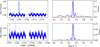 |
Fig. A.1 Time series (left) and GLS periodograms (right) of the TESS photometry of TZ Ari for sectors 70 (top) and 71 (bottom). We mark in purple the stellar rotation period (1.96±0.07 d). |
Statistics on the coefficients derived of ϵ Eri and the corresponding ones for the classical CCF indicators.
Appendix H CANSTAR + Keplerian solution posteriors
We show the posterior distributions from the CANSTAR + Keplerian model.
Statistics on the coefficients derived of TZ Ari and the corresponding ones for the classical CCF indicators.
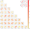 |
Fig. D.1 Correlations between the first 8 decomposition coefficients, colour-coded according to the absolute value of their Pearson correlation coefficient, where the exact value is printed over the image. Strongest correlations with classical CCF indicators appear at CON–c1, RV–l, FWHM–g2, and BIS–g3 (top right). |
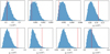 |
Fig. E.1 Histograms showing the distribution of RMS values for the coefficients derived from 10 000 StarSim simulations for ϵ Eri. The RMS values of the actual observed HARPS coefficients are shown by vertical red dashed lines. We apply z-score normalisation to bridge the gap between the time series RMS from the simulated distributions and the observed ones. |
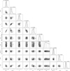 |
Fig. H.1 Posterior distribution from emcee for the CANSTAR + Keplerian solution |
All Tables
Stellar parameters and adopted values for the StarSim simulations for ϵ Eri and TZ Ari.
Statistics on the coefficients derived of ϵ Eri and the corresponding ones for the classical CCF indicators.
Statistics on the coefficients derived of TZ Ari and the corresponding ones for the classical CCF indicators.
All Figures
|
Fig. 1 Time-averaged CCFs (templates) of ϵ Eri (red) and TZ Ari (blue) with the corresponding Gaussian model fit for ϵ Eri (orange) and the two-component Gaussian model fit for TZ Ari (cyan). |
| In the text | |
|
Fig. 2 Time series (left) and GLS periodograms (right) of the RV and activity indicators derived from the CCFs for ϵ Eri. We mark in purple the stellar rotation period (11.2 d) and its first harmonic (5.6 d). The 0.1, 1, and 10% FAP levels are shown with dashed orange lines. |
| In the text | |
|
Fig. 3 Time series (left) and GLS periodograms (right) of the RV and activity indicators derived from the CCF for TZ Ari. The stellar rotation period (1.96 d) is marked in purple; the planetary orbital period from the literature (722.05 d; Quirrenbach et al. 2022) is marked in light blue; and the 0.1%, 1%, and 10% FAP levels are shown with dashed orange lines. The frequency axis of the periodogram show two scales split at 0.035 d−1 to better visualise long-term variability. The RVs display low-frequency signals associated with the Keplerian motion of TZ Ari b, while the CON and FWHM show lower-frequency stellar activity signals. |
| In the text | |
|
Fig. 4 First six basis components for ϵ Eri (Hermite, red) and TZ Ari (multi-Hermite, blue). |
| In the text | |
|
Fig. 5 Explained variance ratio (solid) and cumulative variance (dashed) per component for ϵ Eri (Hermite, red) and TZ Ari (multi-Hermite, blue). |
| In the text | |
|
Fig. 6 Cross-correlation function decomposition of ϵ Eri with a Hermite basis. Left: contribution of consecutive basis components to the differential CCF reconstruction. We displayed six illustrative epochs randomly selected to visualise the temporal variability of the line-shape distortions. The observed differential CCFs are shown in grey, while the reconstructed components are colour-coded according to the observation time. Middle: time series of the corresponding coefficients. Right: GLS periodograms of the coefficients. The 0.1%, 1%, and 10% FAP levels are indicated in orange, and the stellar rotation period and its first harmonic are marked in purple. |
| In the text | |
|
Fig. 7 Same as Fig. 6 but for the multi-Hermite basis applied to TZ Ari. We also mark in light blue the planetary orbital period from the literature (722.05 d; Quirrenbach et al. 2022). |
| In the text | |
|
Fig. 8 Schematic representation of CANSTAR (bottom), a convolutional attention network designed to predict the stellar activity contribution to line shifts, κ(t), from the time series of distortion coefficients, gi(t). The input coefficients are treated as independent channels and processed through a series of one-dimensional convolutional layers that extract local temporal features. The convolutional outputs are then passed to a transformer encoder module, which consists of a multi-head self-attention part (top) with different ‘heads’, where each one of them focuses on different temporal dependencies within the data, and their outputs are combined, normalised, and propagated through additional attention layers. Finally, the resulting features are flattened and projected through a linear layer to produce the predicted κ(t) time series. |
| In the text | |
|
Fig. 9 Residual relative error of ϵ Eri (top) and TZ Ari (bottom) StarSim data after correction with CANSTAR (solid line with circle marker) and an FCN (dashed line with square marker) for the noiseless case (blue) and for the case with noise equivalent to the observations (green). |
| In the text | |
|
Fig. 10 Top: Radial velocity time series (left) and GLS periodogram (right) of the HARPS ϵ Eri data (blue) compared to the stellar activity signal predicted by CANSTAR (green). Bottom: Residuals after subtracting the prediction (grey), with their corresponding periodogram (right). The 10%, 1%, and 0.1% FAP levels are indicated by dashed orange lines and the stellar rotation period (11.2 d), and its first harmonic (5.6 d) is marked in purple. The residuals are compatible with the ϵ Eri b solution (red; Thompson et al. 2025). |
| In the text | |
|
Fig. 11 Detection limits in the ϵ Eri residuals after applying CANSTAR’s correction, shown as a function of the difference between injected and retrieved frequencies (left) and semi-amplitudes (right) for the different injected frequencies and semi-amplitudes sinusoidal signals. |
| In the text | |
|
Fig. 12 Histograms showing the posterior distribution of the shared parameters between the CANSTAR and GP correction methods used to model the TZ Ari RV data. |
| In the text | |
|
Fig. 13 Radial velocity time series and GLS periodograms for TZ Ari showing (a) the complete multi-season dataset and (b) a detailed view of the final observing season. For each panel, the top row displays the CARMENES data (blue), the CANSTAR prediction (green), and the Keplerian solution (red). In the time series, the green curve includes the Keplerian signal to illustrate the full fit, whereas in the periodogram it represents the activity model alone. The bottom row shows the residuals after subtracting both the CANSTAR activity correction and the Keplerian model (grey). The 10%, 1%, and 0.1% FAP levels are indicated by dashed orange lines. The stellar rotation period (1.96 d) is marked with a purple dashed line, and the newly derived planetary orbital period (789.92 d) is marked in light blue (not shown in panel (b) due to its shorter time baseline). |
| In the text | |
|
Fig. 14 Residual time series (left) and GLS periodogram (right) after subtracting the GP + Keplerian model to the TZ Ari RV data (grey). The 10%, 1%, and 0.1% FAP levels are indicated by dashed orange lines. The stellar rotation period (1.96 d) is shown in purple, the newly derived planetary orbital period (789.92 d) is in light blue, and the two signals exceeding the 1% FAP level (37.2 d and 41.4 d) are marked in black. These likely correspond to stellar activity given the significant (40.18 d) periodicity observed in the FWHM and g2 indicators. |
| In the text | |
|
Fig. 15 Top: radial velocity time series (left) and GLS periodogram (right) of the HARPS ϵ Eri data (blue) compared to the stellar activity signal predicted by CANSTAR (green) and Perger et al. (2023, magenta). We note that the Perger et al. (2023) did not provide uncertainties to their NN predictions. Bottom: Residuals after subtracting the prediction with their corresponding periodogram (right). The 10%, 1%, and 0.1% FAP levels are indicated by dashed orange lines. |
| In the text | |
|
Fig. A.1 Time series (left) and GLS periodograms (right) of the TESS photometry of TZ Ari for sectors 70 (top) and 71 (bottom). We mark in purple the stellar rotation period (1.96±0.07 d). |
| In the text | |
|
Fig. D.1 Correlations between the first 8 decomposition coefficients, colour-coded according to the absolute value of their Pearson correlation coefficient, where the exact value is printed over the image. Strongest correlations with classical CCF indicators appear at CON–c1, RV–l, FWHM–g2, and BIS–g3 (top right). |
| In the text | |
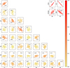 |
Fig. D.2 Same as Fig. D.1 but for the multi-Hermite basis applied to TZ Ari. |
| In the text | |
|
Fig. E.1 Histograms showing the distribution of RMS values for the coefficients derived from 10 000 StarSim simulations for ϵ Eri. The RMS values of the actual observed HARPS coefficients are shown by vertical red dashed lines. We apply z-score normalisation to bridge the gap between the time series RMS from the simulated distributions and the observed ones. |
| In the text | |
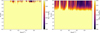 |
Fig. F.1 Same as Fig. 11 but for the null hypothesis case. |
| In the text | |
|
Fig. H.1 Posterior distribution from emcee for the CANSTAR + Keplerian solution |
| In the text | |
Current usage metrics show cumulative count of Article Views (full-text article views including HTML views, PDF and ePub downloads, according to the available data) and Abstracts Views on Vision4Press platform.
Data correspond to usage on the plateform after 2015. The current usage metrics is available 48-96 hours after online publication and is updated daily on week days.
Initial download of the metrics may take a while.