Dust evolution across cosmic times as seen through DUSTY-GAEA

Omima Osman; Gabriella De Lucia; Fabio Fontanot; Lizhi Xie; Michaela Hirschmann

doi:10.1051/0004-6361/202558572

Home

All issues

Volume 710 (June 2026)

A&A, 710 (2026) A306

Full HTML

Open Access

Issue		A&A Volume 710, June 2026


Article Number		A306
Number of page(s)		20
Section		Numerical methods and codes
DOI		https://doi.org/10.1051/0004-6361/202558572
Published online		23 June 2026

A&A, 710, A306 (2026)

Dust evolution across cosmic times as seen through DUSTY-GAEA

Omima Osman¹^,2^★, Gabriella De Lucia¹^,3, Fabio Fontanot¹^,3, Lizhi Xie⁴ and Michaela Hirschmann¹^,5

¹ INAF – Astronomical Observatory of Trieste, via G.B. Tiepolo 11, 34143 Trieste, Italy
² University of Khartoum – Department of Physics, Al-Gamaa Ave, 11115 Khartoum, Sudan
³ IFPU – Institute for Fundamental Physics of the Universe, via Beirut 2, 34151 Trieste, Italy
⁴ Tianjin Astrophysics Center, Tianjin Normal University, Binshuixidao 393, 300384 Tianjin, China
⁵ Institute for Physics, Laboratory for Galaxy Evolution, EPFL, Observatoire de Sauverny, Chemin Pegasi 51, 1290 Versoix, Switzerland

^★ Corresponding author: This email address is being protected from spambots. You need JavaScript enabled to view it.

Received: 15 December 2025
Accepted: 15 April 2026

Abstract

For many decades, dust has been recognised as an important ingredient in galaxy formation and evolution. This paper presents a novel self-consistent implementation of dust formation by stars, destruction by supernova shocks and hot gas, and growth within the dense interstellar medium (ISM) in the state-of-the-art GAEA galaxy formation model. Our new model DUSTY-GAEA is able to reproduce the dust build-up as a function of stellar mass out to z ∼ 6, the scaling relations between the dust-to-gas and dust-to-metal ratios and the stellar mass and metallicity in the local Universe, and the dust mass function both in the local Universe and out to z ∼ 1. In the framework of our model, dust growth dominates the cosmic dust budget out to z ∼ 8, and we find that observational constraints beyond the local Universe can be reproduced only when assuming such efficient dust growth in the dense ISM. Nevertheless, reproducing the estimated number densities of dust-rich galaxies at higher redshifts remains challenging, as also found in independent theoretical work. We discuss our model predictions in comparison with both observational data and independent theoretical efforts, and we highlight how further observational constraints at high redshifts would help constrain dust models.

Key words: stars: formation / dust, extinction / galaxies: evolution / galaxies: ISM

© The Authors 2026

Open Access article, published by EDP Sciences, under the terms of the Creative Commons Attribution License (https://creativecommons.org/licenses/by/4.0), which permits unrestricted use, distribution, and reproduction in any medium, provided the original work is properly cited.

This article is published in open access under the Subscribe to Open model. This email address is being protected from spambots. You need JavaScript enabled to view it. to support open access publication.

1 Introduction

Interstellar dust is a challenging baryonic component to study because of its complex interactions with both the interstellar medium (ISM) and stellar radiation. Dust provides a surface where numerous chemical reactions take place, leading to the formation of various molecules, including molecular hydrogen, which is essential for star formation (Williams 1987; Cazaux & Tielens 2004; Demyk 2011; Dulieu et al. 2013; Bigiel et al. 2008; Schruba et al. 2011). Moreover, collisions between dust grains and gas-phase species result in the depletion of gas-phase metals and cooling and heating of the gas (Black 1987; Draine 2011; Glover & Clark 2012; Klessen & Glover 2016; Zhukovska et al. 2016, 2018).

Dust grains also absorb and scatter stellar UV and optical radiation, re-emitting it in the infrared and submillimetre parts of the electromagnetic spectrum (Draine 2003; Galliano et al. 2018; Bianchi et al. 2018). Furthermore, far-ultraviolet photons can eject energetic electrons from the surfaces of small dust grains (Watson 1972; Draine 1978; Bakes & Tielens 1994; Weingartner & Draine 2001; Wolfire et al. 2003; Hill et al. 2018). These electrons are the main source of heating in the cold neutral medium, and the diffuse atomic hydrogen (HI) regions (Wolfire et al. 1995; Ingalls et al. 2002). In summary, despite its small contribution to the mass budget of galaxies (only 0.1% of the stellar mass; Draine 2007; Smith et al. 2012), dust regulates the rates of chemical reactions that lead to the formation of different molecules in the ISM, chemical abundances, the dynamical and thermodynamical state of galaxies, and their spectral energy distribution.

Our understanding of how dust forms and evolves has developed over decades of observational and theoretical studies. Dust is believed to form mainly in the ejecta of asymptotic giant branch (AGB) stars and type Ia and type II supernovae (SNe; Dwek 1998). Supernovae inject both oxygen-rich and carbon-rich dust into the ISM (e.g. Dwek 1998; Nozawa et al. 2003; Sarangi et al. 2018), while AGB stars produce either oxygen-rich or carbon-rich dust, depending on the ratio of carbon to oxygen in their ejecta (Whittet 1989; Sargent et al. 2010; Srinivasan et al. 2010). Once injected into the ISM, dust grains undergo destruction processes driven by SN remnants and interactions with the hot gas. These processes include sputtering, sublimation, and complete or partial vaporisation (Barlow 1978; McKee 1989; Jones et al. 1994; Nozawa et al. 2006; Bianchi & Schneider 2007; Yamasawa et al. 2011; Andersen et al. 2011; Bocchio et al. 2016).

The dust grains that survive can eventually reach dense regions of the ISM, where they can grow through the accretion of gas-phase metals (Dwek & Scalo 1980; Dwek 1998; Hirashita 2013). Depletion studies strongly support and constrain this mechanism of dust formation (Duley & Millar 1978; Jones & Williams 1985; Savage & Sembach 1996). For example, Zhukovska et al. (2016, 2018) found that dust growth is essential to explaining silicon and iron depletion levels in the Milky Way. Finally, dust grains could shatter or coagulate when they collide with each other, leading to changes in the grain size distribution (e.g. Hirashita 2015).

A large amount of information about dust abundance in galaxies and how it relates to their physical properties has been collected over the past decades. This information includes the scaling relations between dust mass and stellar mass (Corbelli et al. 2012; Santini et al. 2014; Beeston et al. 2018; Nersesian et al. 2019), dust mass and star formation rate (da Cunha et al. 2010; Casey 2012; Santini et al. 2014; Rowlands et al. 2014), the dust mass function (DMF) of galaxies (Dunne et al. 2003, 2011; Vlahakis et al. 2005; Eales et al. 2009; Clemens et al. 2013; Clark et al. 2015; Beeston et al. 2018; Pozzi et al. 2020), the dust-togas (DtoG) ratio versus metallicity (Issa et al. 1990; Lisenfeld & Ferrara 1998; James et al. 2002; Draine et al. 2007; Galametz et al. 2011; Magrini et al. 2011; Hirashita & Kuo 2011; Hirashita 2013; Rémy-Ruyer et al. 2014; Relaño et al. 2018), the dust-tometal (DtoM) ratio versus metallicity (De Cia et al. 2013, 2016; Zafar & Watson 2013; Sparre et al. 2014; Wiseman et al. 2017; Popping & Péroux 2022), and the gas fraction of galaxies versus dust mass (Cortese et al. 2012). This wealth of data can be used to constrain dust models included in theoretical frameworks of galaxy formation.

In the local Universe, dust produced by stars and dust growth appear to play a dominant role in regulating the amount of dust observed and the scaling relations with other physical properties. At high redshift, the situation is less clear, as dust evolution may have proceeded quite differently. For instance, many galaxies appear to be overabundant in dust for their age, with dust masses equal to or exceeding 10⁷ M_⊙ at z > 4 (e.g. Riechers et al. 2014; Watson et al. 2015; Pozzi et al. 2020), representing a challenge for current theoretical models. This discrepancy raises questions about our understanding of the processes that control dust in the early stages of galaxy evolution. For example, it is unclear whether progenitors of AGB stars are effective dust producers at high redshift given the long time-scales involved (see Valiante et al. 2009 for alternative view). It is also unclear whether dust growth continues to be a dominant dust formation channel at high redshift given that the gaseous metallicity decreases at earlier cosmic epochs. The effective stellar yields at high redshift are also unknown and could be significantly different from those measured in the local Universe. Observational data at these earlier cosmic epochs are also limited and potentially affected by systematics and selection effects that we probably still do not fully understand.

In recent years, theoretical models have been updated to include processes that account for the formation, destruction, and growth of dust (e.g. Bekki 2013; McKinnon et al. 2016; Popping et al. 2017; Vijayan et al. 2019; Li et al. 2019; Triani et al. 2020; Yates et al. 2024 ). A few models also include a treatment for the grain size distribution (e.g. Hirashita 2015; Aoyama et al. 2017; Hou et al. 2017; Gjergo et al. 2018; Granato et al. 2021; Parente et al. 2023). These models reproduce reasonably well such properties as the local DMF, the dust mass-stellar mass relation, and the DtoG ratio versus metallicity relation in the local Universe. However, observations at high redshift remain more challenging to reproduce.

In this work, we introduce an updated version of the GAlaxy Evolution and Assembly (GAEA)¹ model that includes an explicit treatment for dust formation, destruction, and growth. The GAEA model is a state-of-the-art semi-analytic model that successfully reproduces a wide range of observational results. Notably, GAEA employs an innovative approach for the non-instantaneous recycling approximation of gas, metals, and energy by SNe and AGBs (De Lucia et al. 2014), resulting in

precise calculations of the ISM metallicity history and providing an ideal framework for the implementation of dust physics. Semi-analytic models are particularly well suited to addressing the challenges involved in dust prescriptions, as they allow for the exploration of a vast parameter space across large cosmological volumes while keeping computational costs reasonable.

The paper is organised as follows: Section 2 presents our dust model and its variants. Results are detailed in Sect. 3. Our discussion and summary are presented in Sects. 4 and 5, respectively.

2 DUSTY-GAEA

In this work, we use the Millennium (Springel et al. 2005; MSI) and Millennium II (Boylan-Kolchin et al. 2009; MSII) simulations. These model boxes with a side length of 500 and 100 Mpch⁻¹, respectively, and assume the following cosmological parameters: Ω_Λ = 0.75, Ω_m = 0.25, Ω_b = 0.045, n = 1, σ₈ = 0.9, and h = 0.73. The MSI contains 2160³ particles and achieves a resolution of 8.61×10⁸ M_⊙, while MSII contains the same number of particles and achieves a resolution of 6.89×10⁶ M_⊙. The cosmological parameters adopted here differ from those from the Planck (Planck Collaboration XIII 2016) and WMAP9 (Bennett et al. 2013) results. The impact on model predictions is expected to be minimal as demonstrated by Wang et al. (2008) and Guo et al. (2013). Indeed, Fontanot et al. (2025) showed that GAEA predictions converge well for runs using merger trees extracted from simulations at different resolutions and slightly different cosmological parameters, ranging from WMAP1 to Planck values.

Our starting reference model version is the one described in De Lucia et al. (2024). This model represents a significantly modified and extended version of the original model by De Lucia & Blaizot (2007). In particular, it includes an updated parameterisation of stellar feedback (Hirschmann et al. 2016), a partition of cold gas into atomic and molecular components (Xie et al. 2017), a gradual stripping of the hot and cold gas from satellite galaxies (Xie et al. 2020), and an improved model for cold gas accretion onto black holes and explicit modelling of quasar driven winds (Fontanot et al. 2020). Particularly relevant for this study is the innovative treatment of the non-instantaneous recycling of gas, energy, and metal (De Lucia et al. 2014). The model is calibrated to reproduce several observables, including the stellar mass function up to redshift ~3, the HI and H₂ mass function in the local Universe, and the active galactic nucleus (AGN) bolometric luminosity function up to redshift ~4 (see e.g. De Lucia et al. 2024). In the following we provide a summary of the GAEA prescriptions mostly relevant for this work. For full details on these implementations, we refer the reader to the original papers.

In summary, GAEA assumes that baryons are distributed in four different reservoirs: stars within galaxies, cold gas in galaxy discs (representing the ISM), hot gas associated with centrals and satellites, and ejected gas that has been reheated and expelled from halos by SNe- and AGN-driven winds. This ejected gas can later be reincorporated into the hot gas component (Hirschmann et al. 2016; Xie et al. 2020). Metals are always assumed to follow the circulation of baryons between the different reservoirs. For example, metals are locked into stars when they are formed, keeping the metallicity of the ISM constant. In the model, DUSTY-GAEA, presented in this work, we have introduced three additional dust reservoirs, corresponding to each of the gas reservoirs: dust in the cold gas, dust in the hot gas, and dust in the ejected gas. As for metals, dust is also assumed to follow the circulation of baryons between the different reservoirs.

As described in detail in De Lucia et al. (2014), chemical enrichment is modelled by projecting the information about the metals, gas and energy produced by each simple stellar population (SSP) in the future. This approach allows for an accurate accounting of the timings and properties of the individual SSPs in model galaxies. The reference model adopts a Chabrier initial mass function (IMF; Chabrier 2003)² and makes use of the stellar yield tables by Karakas (2010) for low- and intermediatemass stars, Thielemann (2003) for SNeIa, and Chieffi & Limongi (2004) for SNeII. The yields by Chieffi & Limongi (2004) are defined for stellar masses between 13 and 35 M_⊙. Between 8 and 13 M_⊙, the yields are scaled proportionally to the stellar mass, while for more massive stars, the values corresponding to the highest stellar mass tabulated are used. In our version of the model, we have modified the code to follow explicitly the abundance of ten chemical elements (H, He, Mg, Si, O, C, Fe, S, Ca, Ti), and the chemical enrichment scheme such that all the metals are released into the cold gas regardless of the halo mass (see also Cantarella et al. 2025).

Taking advantage of the accurate approach to model chemical evolution included in GAEA, we implement an explicit model for the formation and evolution of dust. The dust model adopted consists of (i) dust formation in stellar winds of AGB stars, SNIa, and SNII, (ii) accretion of the ISM gas-phase metals on dust grains, i.e. dust growth, and (iii) dust destruction by SN remnants and sputtering in the hot gas. These processes are the main drivers of the dust mass evolution (Hirashita 2013) and their implementation is described in the following subsections.

2.1 Dust formation by stars

The total mass of the jth element (j = C, O, Mg, Si, S, Ca, Fe, Ti) in dust from the kth type of stars (SNIa, SNII, and AGB stars) can be expressed as (Dwek 1998): $m_{d u s t, j}^{k} = δ_{c, j}^{k} F_{e j} (m_{e j, j}^{k}),$ $Mathematical equation: m_{\rm dust, \it j}^k= \delta_{\rm c, \it j}^k F_{\rm ej}(m_{\rm ej, \it j}^k),$ (1)

where $δ_{c,, j}^{k}$ $Mathematical equation: $\delta_{\rm c, \it, j}^k$$ is the fraction of the jth chemical element from the kth stellar type locked up in dust grains (i.e. the condensation efficiency), F_ej is a function determining the total mass of metals that can be used for dust formation, and mj is the mass of the jth element ejected from the kth stellar type.

2.1.1 Dust from AGB stars

Depending on whether the stellar ejecta is carbon- or oxygenrich, the dust produced by AGB stars would be carbon rich or oxygen rich, respectively. This is because oxygen and carbon combine to form the maximum possible amount of CO, and as such either one of the two would be unavailable for dust formation by the end of the CO formation process (Dwek 1998). Following previous works, we considered the two cases described below.

Case 1: C/O > 1, Carbon-rich dust $m_{d u s t, C}^{A G B} = δ_{c, C}^{A G B} (m_{e j, C}^{A G B} - 0.75 m_{e j, O}^{A G B}),$ $Mathematical equation: m_{\rm dust, \it C}^{AGB}= \delta_{\rm c, \it C}^{AGB} (m_{\rm ej, \it C}^{AGB} - 0.75m_{\rm ej, \it O}^{AGB}), \\$ (2) $m_{d u s t, j}^{A G B} = 0,$ $Mathematical equation: m_{\rm dust, \it j}^{AGB} = 0,$ (3)

where j = O, Mg, Si, S, Ca, Fe, Ti.

Case 2: C/O < 1, Oxygen-rich dust $m_{d u s t, C}^{A G B} = 0,$ $Mathematical equation: m_{\rm dust, \it C}^{AGB} = 0,\\$ (4) $m_{d u s t, j}^{A G B} = δ_{c, j}^{A G B} m_{e j, j}^{A G B},$ $Mathematical equation: m_{\rm dust, \it j}^{AGB}= \delta_{\rm c, \it j}^{AGB} m_{\rm ej, \it j}^{AGB}, \\ \label{eq6}$ (5) $m_{d u s t, O}^{A G B} = 16 \times \sum_{j} δ_{c, j}^{A G B} m_{e j, j}^{A G B} / μ_{j},$ $Mathematical equation: m_{\rm dust, \it O}^{AGB}= 16 \times \sum_j \delta_{\rm c, \it j}^{AGB} m_{\rm ej, \it j}^{AGB}/\mu_j,$ (6)

where j = Mg, Si, S, Ca, Fe, Ti and μj is the atomic mass of element j.

2.1.2 Dust from SNIa and SNII

Supernovae produce both carbon- and oxygen-rich dust since the macro-mixing of their ejecta allows the presence of carbon- and oxygen-rich regions (Nozawa et al. 2006). We assumed $m_{d u s t, j}^{S N I a - S N I I} = δ_{c, j}^{S N I a - S N I I} m_{e j, j}^{S N I a - S N I I},$ $Mathematical equation: m_{\rm dust, \it j}^{SNIa-SNII}= \delta_{\rm c, \it j}^{SNIa-SNII} m_{\rm ej, \it j}^{SNIa-SNII}, \\\label{eq8}$ (7) $m_{d u s t, C}^{S N I a - S N I I} = δ_{c, C}^{S N I a - S N I I} m_{e j, C}^{S N I a - S N I I},$ $Mathematical equation: m_{\rm dust, \it C}^{SNIa-SNII}= \delta_{\rm c, \it C}^{SNIa-SNII} m_{\rm ej, \it C}^{SNIa-SNII}, \\\label{eq9}$ (8) $m_{d u s t, O}^{S N I a - S N I I} = 16 \times \sum_{j} δ_{c, j}^{S N I a - S N I I} m_{e j, j}^{S N I a - S N I I} / μ_{j},$ $Mathematical equation: m_{\rm dust, \it O}^{SNIa-SNII}= 16 \times \sum_j \delta_{\rm c, \it j}^{SNIa-SNII} m_{\rm ej, \it j}^{SNIa-SNII}/\mu_j,$ (9)

where j = Mg, Si, S, Ca, Fe, Ti.

We adopted $δ_{c, j}^{S N I a - S N I I}$ $Mathematical equation: $\delta_{\rm c, \it j}^{SNIa-SNII}$$ = 0.15 for all elements produced by SNIa and SNII and $δ_{c, j}^{A G B}$ $Mathematical equation: $\delta_{\rm c, \it j}^{AGB}$$ = 0.2 for all elements produced by AGB stars (Popping et al. 2017). These low condensation efficiencies account for inefficiency in dust production and dust destruction during ejection into the ISM by the reverse SN shock (Popping et al. 2017; Micelotta et al. 2018). Some observational and theoretical studies have shown that dust produced by SNIa is minimal (see e.g. Gioannini et al. 2017; Li et al. 2019; Parente et al. 2022). Switching off their contribution, we also find a negligible contribution of SNIa to our predicted dust budget; as such, we keep their contribution in the present work.

We also tested the original Dwek (1998) condensation efficiencies, namely $δ_{c, j}^{S N I a - S N I I}$ $Mathematical equation: $\delta_{\rm c, \it j}^{SNIa-SNII}$$ = 0.5 for carbon and 0.8 for all the other elements produced by SNIa and SNII, and $δ_{c, j}^{A G B}$ $Mathematical equation: $\delta_{\rm c, \it j}^{AGB}$$ = 1. However, for the set of metal yields we adopted, the oxygen-rich dust produced adopting those efficiencies exceeds the available oxygen. We lowered the constant factor in Eqs. 6 and 9 from 16 to 10, following McKinnon et al. (2016); however, the problem was not resolved.

Adopting a constant condensation efficiency is a simplification of the formation process. Indeed, stellar evolution studies indicate varying dust condensation efficiencies with the initial mass of stars and metallicity (e.g. Ferrarotti & Gail 2006). This and the uncertainties in the stellar metal yields and the IMF could significantly influence the amount of dust produced by stars. We will study this in more detail in future work.

2.2 Dust destruction

Once dust is injected into the ISM, it experiences several destructive processes, including thermal and non-thermal sputtering (McKee 1989; Jones et al. 1994; Jones 2004; Hirashita 2013). Sputtering is caused by the high-velocity collisions between the gas phase atoms and ions with the dust grains. Thermal sputtering results from the random thermal motion of the gas species, as in the case of the hot gas in galaxy halos. Meanwhile, nonthermal sputtering arises from the relative motion between the gas and dust grains, as in the case of SNe forward shock waves. Metals removed from the dust grains are recycled to the ISM upon destruction. In the following, we describe our treatment of both processes.

2.2.1 Destruction by SNe forward shocks

To model dust destruction by SNe, one needs to take into account a) the energy and evolution of the exploding SN, b) the properties of the ISM in which SN events occur (i.e. density and metallic-ity), and c) the properties of the dust in this ISM (i.e. composition and grain size). Furthermore, ISM regions are often subject to several SNe explosions, and the total amount of dust destroyed in a region should be computed as the integral of the dust destroyed by all ‘overlapping’ events. In practice, the problem is typically simplified by estimating the dust destroyed by a single event and then multiplying by the SNe rate corrected for SNe clustering.

We followed the approach described in McKee (1989) to estimate the characteristic timescale of the process, the destruction timescale, τ_des, $τ_{d e s} = \frac{M_{H I + H I I}}{M_{s w e p t} γ_{S N} ξ_{S N} ζ_{S N}} y r,$ $Mathematical equation: \tau_{des} = \frac{M_{HI+HII}}{M_{swept} \gamma_{SN} \xi_{SN} \zeta_{SN}} \rm yr,$ (10)

where $M_{s w e p t} = 6800 (\frac{v_{s}}{100 k m s^{- 1}}) (\frac{E_{S N}}{10^{51} e r g}) M_{⊙},$ $Mathematical equation: M_{swept} = 6800\left(\frac{v_s}{100 \rm kms^{-1}}\right)\left(\frac{E_{SN}}{10^{51}\rm erg}\right) M_{\odot} ,$ (11)

and $v_{s} = 200 {(\frac{n_{0}}{1 c m^{- 3}})}^{\frac{1}{7}} (\frac{E_{S N}}{10^{51} e r g}) k m s^{- 1} .$ $Mathematical equation: v_s = 200\left(\frac{n_0}{1 \rm cm^{-3}}\right)^{\frac{1}{7}}\left(\frac{E_{SN}}{10^{51}\rm erg}\right) \rm kms^{-1}.$ (12)

In these equations, M_HI+HII is the mass of the atomic and ionised gas, M_swept is the mass of the ISM swept up by the shock wave, γ_SN is SNe rate, ξ_SN is the fraction of clustered SNe (= 0.36, McKee 1989), and ζ_SN is a single SN destruction efficiency (= 0.34, Nozawa et al. 2006). v_s is the shock velocity, E_sn is the energy of a single SN event, and n₀ is the ambient gas density. We estimate γ_SN using the total energy released by SNIa and SNII events in each time step divided by the energy released in a single event (~10⁵¹ ergs).

Most of the dust destruction is expected to occur in the warm intercloud medium (McKee 1989); accordingly, we allowed dust destruction only in this medium. Hence, we estimated n₀ using all the cold gas mass that is not in molecular form (for details about how the cold gas component of model galaxies is partitioned into different components, we refer the reader to the original paper by Xie et al. 2017) and the volume, V₀, occupied by this gas. We computed V₀ as the volume of the galaxy disc multiplied by one minus the H₂ volume-filling factor (f_v,H₂ ~ 0.001, Table 1.3 in Draine 2011). Figure 1 (top panel) shows n₀ distribution up to redshift 5.5 for the MSI runs (MSII runs yield similar results). The mass we used in the calculation is slightly overestimated since our calculation does not account for the presence of gas phases other than the warm ionised and the cold molecular. Therefore, we imposed an upper limit on the gas density consistent with what is reported in Draine (2011), 1 cm⁻³.³

The same approach is used to estimate the density of the molecular gas (n_H, Fig. 1 bottom panel), where V₀ is computed as the volume of the galaxy disc multiplied by H₂ volume-filling factor. It is worth noting that the H₂ volume-filling factor we adopted here is an estimation in the Milky Way and might not be the same in all galaxies at all redshifts. We adopt this approach trying to account for the redshift evolution of the ISM density instead of imposing a fixed density.

The change in mass of the element j in dust due to SNe destruction in the warm component of the cold gas was then estimated using the following equation from Dwek (1998): $Δ m_{d u s t, j}^{d e s} (t) = - Δ t m_{d u s t, j} (t) / τ_{d e s},$ $Mathematical equation: \Delta m_{dust, j}^{des}(t)= - \Delta t \, m_{dust, j}(t) /\tau_{des},$ (13)

where Δt is the integration time step and m_dust,j(t) is the mass of the jth element already in dust. The same amount of metals removed from the dust phase, $Δ m_{d u s t, j}^{d e s}$ $Mathematical equation: $\Delta m_{dust,j}^{des}$$ , is added to the metals in the (cold)gas phase: $Δ m_{m e t a l, j} (t) = Δ m_{d u s t, j}^{d e s} (t) .$ $Mathematical equation: \Delta m_{metal, j}(t) = \Delta m_{dust, j}^{des}(t).$ (14)

We also tested the model adopted by Popping et al. (2017), Vijayan et al. (2019), and Yates et al. (2024) based on the concept of the mass of the ISM cleared of dust, rather than the dust destruction efficiency. Furthermore, we tested the metallicity-dependent destruction model adopted by Triani et al. (2020) and Parente et al. (2023) but still allowed the density of the gas to vary. Both models show similar destruction efficiency compared to our fiducial model (see Appendix A for further details).

Fig. 1

Normalised histograms of the estimated density of the warm intercloud medium (top) and cold molecular gas (bottom) from z ∼ 0 to z ∼ 5.5. Predictions are based on the MSI merger trees. We limited the distributions to resolved galaxies (see Sect. 3 for details).

2.2.2 Destruction by thermal sputtering

We implemented thermal sputtering in both the hot and the ejected gas reservoirs, following the prescriptions by McKinnon et al. (2017) for the thermal sputtering timescale. This is based on the original formulation introduced by Tsai & Mathews (1995): $τ_{s p u} = 0.17 (\frac{\bar{a}}{0.1 μ m}) (\frac{10^{- 27}}{ρ}) [{(\frac{2 \times 10^{6}}{T})}^{2.5} + 1] G y r,$ $Mathematical equation: \tau_{spu} = 0.17 \left(\frac{\bar{a}}{0.1\mu m}\right) \left(\frac{10^{-27}}{\rho}\right) \left[\left(\frac{2\times 10^6}{T}\right)^{2.5} + 1\right] \rm Gyr ,$ (15)

where ρ is the gas density in g cm⁻³ units, and T is the temperature in K. The hot gas reservoir contains all gas with a temperature above 10⁴ K and is assumed to be in isothermal equilibrium. For the calculation of the sputtering rate, however, we assume that the gas temperature is equal to the virial temperature and that the gas follows a homogeneous spherical density profile bounded by the virial radius, which is used to estimate the gas density (i.e. $ρ = M_{h o t} / \frac{4}{3} π R_{v i r}^{3}$ $Mathematical equation: $\rho$ = $M_{\rm hot}/\frac{4}{3}\pi R_{\rm vir}^{3}$$ ). We further assume ā = 0.1 μm for the average grain size. The ejected reservoir is assumed to have the same properties as the hot reservoir, except that it is decoupled from cooling for a brief period of time (Croton et al. 2006; De Lucia et al. 2010). Therefore, we applied the same sputtering rate in both reservoirs. Accordingly, the change in mass of the element j in dust due to sputtering in the hot or ejected gas is $Δ m_{d u s t, j}^{s p u} (t) = - Δ t m_{d u s t, j} (t) / 3 τ_{s p u} .$ $Mathematical equation: \Delta m_{dust, j}^{spu}(t)= - \Delta t \, m_{dust, j}(t)/3\tau_{spu}.$ (16)

The same amount, $Δ m_{d u s t, j}^{s p u}$ $Mathematical equation: $\Delta m_{dust,j}^{spu}$$ , is added to the (hot or ejected)gas phase metals.

2.3 Dust growth in dense media

Dust destruction by SNe is a rather efficient process, where only about 10 to 20 per cent of the dust survives (McKee 1989; Dwek 1998). The remaining dust could hardly account for the vast amounts of dust observed in the local and distant Universe (Jones et al. 1994; Bertoldi et al. 2003; Mattsson 2011; Kuo & Hirashita 2012; McKinnon et al. 2016, 2018; Ginolfi et al. 2018; Shivaei et al. 2024). To alleviate this tension, an efficient additional source of dust must be present. Dwek & Scalo (1980) proposed dust growth via accretion of the gas phase metals in the dense metal-rich regions of the ISM as a viable process. Studies of ISM depletions strongly support and constrain this scenario (Duley & Millar 1978; Jones & Williams 1985; Savage & Sembach 1996; Zhukovska et al. 2016, 2018). Theoretical studies also support dust growth as a viable mechanism to explain observations (e.g. Dwek 1998; Bekki 2013; Aoyama et al. 2017; Popping et al. 2017).

Considering the uncertainties related to the modelling of this specific process, we adopt two frameworks to implement dust growth in our galaxy formation model. These are based on the formalisms introduced in Dwek (1998) and Zhukovska et al. (2008). Both frameworks follow the evolution of the dust mass, omitting the evolution of its grain size distribution. However, unlike the Dwek framework, Zhukovska et al. take into account the dust grain composition, allowing us to have predictions of oxygen depletion of about ~0.03-0.2, consistent with the depletion level adopted in emission-line modelling studies (e.g. Groves et al. 2004; Gutkin et al. 2016).

2.3.1 Dwek framework

The growth timescale varies according to the ISM properties (i.e. density, temperature and metallicity) and the grain size. We used the following formula by Asano et al. (2013b): $C_{s} τ_{a c c, j} = 2 \times 10^{7} (\frac{\bar{a}}{0.1 μ m}) {(\frac{n_{H}}{100 c m^{- 3}})}^{- 1} {(\frac{T}{50 K})}^{- \frac{1}{2}} {(\frac{Z_{j}}{Z_{⊙}})}^{- 1} y r,$ $Mathematical equation: C_s \tau_{\rm acc, \it j} = 2\times 10^7 \left(\frac{\bar{a}}{0.1\mu \rm m}\right) \left(\frac{n_{H}}{100\rm cm^{-3}}\right)^{-1} \left(\frac{T}{50 \rm K}\right)^{-\frac{1}{2}} \left(\frac{Z_j}{Z_\odot}\right)^{-1} \rm yr ,$ (17)

where C_s (= 1) is the dust sticking coefficient, the probability that a metal atom or ion sticks to the dust grain after colliding, and Z_j is the abundance ratio of the element j. We modelled the increase in dust mass due to the growth using a slightly modified form of the formula by Dwek (1998) (Popping et al. 2017; Triani et al. 2020): $Δ m_{d u s t, j}^{a c c} (t) = Δ t (1 - f_{d u s t, j}) m_{d u s t, j} (t) f_{H_{2}} / τ_{a c c, j} .$ $Mathematical equation: \Delta m_{dust,j}^{\rm acc}(t)=\Delta t (1-f_{\rm dust, j}) m_{dust,j}(t) f_{H_2}/\tau_{\rm acc, j}.$ (18)

Here, f_dust,j is the fraction of the jth element that is locked up in dust, and f_H₂ is the molecular hydrogen fraction as calculated in Xie et al. (2017). We adopted 0.1 μm and 50 K for the grain size and the cold gas temperature, respectively. We estimated the cold-molecular gas density following the same approach used to estimate the density for SNe destruction (see Sect. 2.2.1 and Fig. 1).

The dust growth process leads to a depletion of the gas phase elements. Accordingly, the mass of the jth element in the gas decreases by $Δ m_{d u s t, j}^{a c c} (t)$ $Mathematical equation: $\Delta m_{dust,j}^{\rm acc}(t)$$ .

2.3.2 Zhukovska et al. (2008) framework

This framework also takes into account the recycling of the gas between the different phases in the ISM. It introduces an effective exchange timescale in which all the ISM is cycled through the molecular phase: $τ_{e x c h, e f f} = \frac{τ_{e x c h \times (1 - f_{H_{2}})}}{f_{H_{2}}} .$ $Mathematical equation: \tau_{exch, eff} = \frac{\tau_{exch\times(1-f_{H_2})}}{f_{H_2}}.$ (19)

Here, τ_exch is the lifetime of molecular clouds (=20 Myrs; Murray & Rahman 2010). The increase in the dust mass due to growth is then estimated using the following equation: $Δ m_{d u s t, j}^{a c c} (t) = Δ t (f_{j, c o n} M_{m e t a l s, j} (t) - m_{d u s t, j} (t)) / τ_{e x c h, e f f},$ $Mathematical equation: \Delta m_{dust,j}^{\rm acc}(t)=\Delta t (f_{j, con}M_{metals,j}(t) - m_{dust,j}(t))/\tau_{\rm exch, eff},$ (20)

where $f_{j, c o n} = {[{(f_{j, 0} (1 + \frac{τ_{e x c h}}{τ_{a c c}}))}^{- 2} + 1]}^{\frac{- 1}{2}},$ $Mathematical equation: f_{j, con} = \left[\left(f_{j,0}\left(1+\frac{\tau_{exch}}{\tau_{acc}}\right)\right)^{-2} + 1\right]^{\frac{-1}{2}},$ (21)

and $τ_{a c c} = 46 \times \frac{b_{d u s t} A_{m e t a l s}^{\frac{1}{2}}}{A_{d u s t}} (\frac{ρ_{d u s t}}{3 g c m^{- 3}}) (\frac{3.5 \times 10^{- 5}}{Z_{j}}) (\frac{10^{3} c m^{- 3}}{n_{H}}) M y r .$ $Mathematical equation: \tau_{acc} = 46 \times \frac{b_{dust}A_{metals}^{\frac{1}{2}}}{A_{dust}}\left(\frac{\rho_{dust}}{3 \rm gcm^{-3}}\right)\left(\frac{3.5\times10^{-5}}{Z_j}\right)\left(\frac{10^3 \rm cm^{-3}}{n_H}\right) \rm Myr .$ (22)

The term f_j,con is the condensation degree of a metal species j at the end of the cloud lifetime, i.e. the mass fraction of the species j condensed into dust, and f_j,0 is the initial condensation degree. The term M_metals,j is the total mass of the jth element in the gas and dust; ρ_dust is the dust grain bulk density; and b_dust, A_metais, and A_dust are parameters determined by the dust grain composition. Following Zhukovska et al. (2008), we adopted carbon dust, silicates (Olivine and Pyroxene with Olivine fraction of 0.32), silicon carbide and metallic iron as dust grain species. Thus, we adopted the same parameter values adopted in the original paper (also shown in Table 1. See also Sect. 4.3 of Zhukovska et al. 2008). Equation (22) is derived averaging with respect to the Mathis, Rumpl, and Nordsieck (MRN) grain size distribution (Mathis et al. 1977).

Table 1

Parameter values for the dust growth model based on the Zhukovska et al. (2008) model.

Table 2

Main characteristics of the dust models presented in this work.

3 Results

In this section we present the main dust scaling relations, the DMF, and the dust cosmic evolution predicted by three variants of our dust model. As our fiducial model, we chose the model that adopts the Zhukovska et al. (2008) framework for dust growth. We refer to this model as ‘DUSTY-GAEA’ in the following. We justify this choice later in the text. Along with DUSTY-GAEA, we discuss two other model variants: DUSTY-GAEA-Dwek, adopting the Dwek framework for dust growth, and a model where dust growth is switched off, DUSTY-GAEA-NoG. Table 2 presents the main characteristics of the three models. In our analysis, we include all galaxies above 10^8.5 M_⊙ from the MSI simulation and galaxies between 10⁷ and 10^8.5 M_⊙ from the MSII simulation. We followed Yates et al. (2024) in combining predictions from MSI and MSII, weighting each galaxy by the inverse of the effective volume of the underlying N-body simulation. We note that discontinuities at the transition region between the two simulations are still visible in at least some scaling relations.

3.1 Dust properties versus stellar mass

The dust mass-stellar mass relation from redshift 0 to ~5.5 is shown in Fig. 2. The solid olive lines represent the median predictions from our fiducial model (DUSTY-GAEA), while the dashed and dash-dotted lines correspond to predictions from DUSTY-GAEA-Dwek and DUSTY-GAEA-NoG, respectively. Shaded areas represent the 16th-84th percentile region. Symbols denote observational data from various sources, including Clark et al. (2015), Rémy-Ruyer et al. (2015), Grossi et al. (2015), De Vis et al. (2019), Nersesian et al. (2019), Beeston et al. (2018), and Santini et al. (2014) at z ~ 0; Rowlands et al. (2014), da Cunha et al. (2015), and Santini et al. (2014) for z between ~1.6 and 2.45; and Rowlands et al. (2014) and da Cunha et al. (2015) at higher redshifts. The ALPINE data from Pozzi et al. (2020) are at redshifts ~4.5 and 5.5. Filled symbols indicate dust mass estimates using a dust temperature of 25 K, while the empty ones indicate estimates using a temperature of 35 k. The blue solid line at z ~ 0 represents the median of the observational data.

All three model variants predict an increase in dust mass as a function of stellar mass across all redshifts⁴. At z ~ 0, the relation bends down beyond a stellar mass of 10¹⁰ M_⊙. Including only star-forming galaxies would remove this bend, indicating that this bend is driven by the influence of passive galaxies in these high stellar mass bins. Unlike star-forming galaxies, these passive galaxies contain most of their gas in the hot gas reservoir, where dust is destroyed via sputtering. In our model, sputtering destroys dust in the hot gas less efficiently than SNe do in the cold gas, consistent with previous studies showing that only 1020% of the dust produced by stars can survive destruction by SNe in the absence of growth (e.g. McKee 1989; Dwek 1998), while 25-33% of the dust survives sputtering (e.g. Aoyama et al. 2018). Nonetheless, gas transfer to the hot reservoir through stellar and AGN feedback depletes the cold gas, which represents the ISM. Therefore, in these galaxies, dust destruction by SNe, together with cold gas depletion, plays a significant role in reducing the dust abundance.

At higher redshifts, the model DUSTY-GAEA-Dwek shows similar bending, which is due to a higher destruction efficiency in this case. In contrast, the model DUSTY-GAEA does not exhibit such bending at higher redshifts. This is because the dust growth model in DUSTY-GAEA is more efficient and able to counterbalance destruction by SNe up to high stellar masses (SNe rate increases with stellar mass and hence dust destruction). Generally, the different growth (and destruction) recipes we tested differ only slightly in their dust mass predictions for low-mass galaxies. At the high mass end, there may or may not be a bend in the relation depending on the specific assumptions. The model with no growth shows a flattening of the relationship above stellar mass of 10⁸ M_⊙ across a larger stellar mass range. In this model, the production by stars is very efficient in increasing the dust mass at low stellar masses, where destruction is still relatively inefficient. As the stellar mass increases the two processes, formation and destruction, come to some sort of equilibrium resulting in the flattening. The gap between this model and the other models increases with stellar mass and redshift. At z ~ 0, the trend of the observational data is well reproduced by the medians of the model variants DUSTY-GAEA and DUSTY-GAEA-Dwek. Beyond redshift zero, the DUSTY-GAEA variant performs better in reproducing observations up to z ~ 5.5. The DUSTY-GAEA-Dwek model trend starts declining about 0.40.8 dex in stellar mass before the DUSTY-GAEA trend stops, limiting the model’s ability to reproduce the dust mass of galaxies in the high stellar mass end. It is intriguing to note that these two model variants predict different dust abundances in these massive galaxies. These two models are conceptually different, particularly in their treatment of the ISM and dust composition (see Sect. 2.3), which leads to these differences.

Dust abundance in galaxies is estimated through several methods, but they primarily fall into two main approaches. The first approach assumes that galaxies behave as optically thin sources with either single or double temperatures, where infrared spectral energy distributions of both local and high-redshift galaxies are typically modelled using a one- or two-component modified blackbody. The second approach uses more complex dust models, such as those by Draine (2007), that account for both a varying radiation field heating the dust and different dust compositions. Both approaches carry uncertainties, up to a factor of three (see Popping et al. 2017; Vijayan et al. 2019; Triani et al. 2020 for more details). The observational data presented here encompass both approaches and these methodological differences - as well as their associated uncertainties - should be kept in mind when compared to our model predictions. Furthermore, data from da Cunha et al. (2015), Santini et al. (2014), and Rowlands et al. (2014) are biased toward bright, relatively high star-forming galaxies, as these studies focus on submillimetre galaxies. Studies focused on Damped Lyman Alpha (DLA) systems such as De Cia et al. (2016), Wiseman et al. (2017), and Péroux & Howk (2020) indirectly infer dust properties at high-z using absorption lines of the gas phase species, adding another layer of systematic errors and uncertainties. Due to the diverse observations presented in this work and the diverse origins of errors and systematic errors carried by them, we did not attempt to convolve our model predictions with any observational errors.

It is evident from the comparison between the three model variants that dust growth is an important process for enriching galaxies at all redshifts but not necessarily at all stellar masses. To understand the relative importance of growth, we studied the dust formation, destruction and growth rates for each model. We show results from DUSTY-GAEA in Fig. 3. The rates based on the DUSTY-GAEA-Dwek model version are very similar, and shown for completeness in Appendix B. In Fig. 3, solid-dashed, solid and dashed-dotted lines show the dust formation rates by stars, destruction by SNe forward shocks, and growth in the dense ISM, respectively. The rates of dust formation by stars and growth in the ISM are similar at low stellar masses, while they are about two orders of magnitude apart at the high stellar mass end, indicating an increasing efficiency of dust growth with stellar mass. The formation rate increases linearly with the stellar mass (a slope between 0.94 and 1.2 depending on the redshift), while the growth rate increases slightly more steeply with stellar mass (a slope between 1.34 and 1.46 depending on the redshift). The destruction rate follows closely the dominant formation process, which is growth. Rates in the DUSTY-GAEA-Dwek model behave similarly, except that the growth trends are a bit steeper (a slope between 1.30 and 1.73 depending on the redshift). In both models, rates of dust formation by stars could hardly exceed the growth in the ISM rates.

Figure 4 presents the DtoG ratio versus stellar mass relation from redshift 0 to ~5.5. Line styles and shaded areas have the same meaning as in Fig. 2, while symbols represent observational data from Grossi et al. (2015), Nersesian et al. (2019), and De Vis et al. (2019). Open symbols correspond to cases where only atomic hydrogen was used to estimate the total gas mass. Both DUSTY-GAEA and DUSTY-GAEA-Dwek models feature a weak increase in the DtoG ratio as a function of stellar mass.

Nonetheless, they differ in their detailed trends. Both models reproduce the observational data in the local Universe well with a comparable scatter. In contrast, DUSTY-GAEA-NoG predicts a decreasing DtoG ratio with stellar mass except for redshift zero, where it significantly underpredicts the observed DtoG ratios.

Figure 5 displays predictions for the DtoM ( $\frac{M_{d}}{M_{d} + M_{m}}$ $Mathematical equation: $\frac{M_d}{M_d + M_m}$$ , where M_m is the total mass of metals in the gas phase) ratio normalised to the Milky Way value (i.e. 0.44) versus stellar mass. Line styles and shaded areas have the same meaning as in Fig. 2, and symbols correspond to observational data from Grossi et al. (2015) and De Vis et al. (2019). Open symbols indicate cases where only atomic hydrogen was used to estimate the gas mass. The blue lines represent model predictions by Vijayan et al. (2019), who included dust formation and evolution models in the semi-analytical galaxy formation model L-Galaxies. This model was run on the same N-body simulations considered in this study. The authors have studied in detail the DtoM ratio.

Following Popping et al. (2017), we estimated the total metal abundance using the 12+log(O/H) values reported by Grossi et al. (2015) and De Vis et al. (2019). The DtoM ratio trends are slightly shallower than the DtoG ratio trends across all redshifts. As the DtoG ratio, which decreases slightly with redshift in the fiducial model, the DtoM ratio also decreases slightly with redshift in both DUSTY-GAEA and DUSTY-GAEA-Dwek models. However, the DtoM ratio and the DtoG ratio share the same features. The DUSTY-GAEA and DUSTY-GAEA-Dwek models perform similarly well in comparison to the observational data. The model by Vijayan et al. (2019) predicts slightly shallower trends than our fiducial model and the opposite redshift evolution, i.e. the DtoM ratio trend decreases with redshift. Our model predicts a slightly higher DtoM ratio down to redshift ~3.5, a similar ratio at ~2.5 and 1.6, and a lower ratio in the local Universe. Generally, our model predicts much weaker redshift evolution.

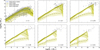Fig. 2

Dust mass as a function of the stellar mass at different redshifts. The solid olive lines represent the median predictions from our fiducial model (DUSTY-GAEA), while the dashed and dash-dotted lines correspond to predictions from DuSTY-GAEA-Dwek and DUSTY-GAEA-NoG, respectively. Shaded areas represent the 16th-84th percentile region. The solid vertical lines indicate the transition between predictions based on MSII and MSI. Symbols represent observational data from Clark et al. (2015, crosses), Rémy-Ruyer et al. (2015, squares), Grossi et al. (2015, upward triangles), De Vis et al. (2019, hexagons), Nersesian et al. (2019, rightward triangles), Beeston et al. (2018, leftward triangles), Santini et al. (2014, diamonds), Rowlands et al. (2014, circles), da Cunha et al. (2015, stars), and Pozzi et al. (2020, downward triangles).

Fig. 3

Dust formation, destruction, and growth rates as predicted by the DUSTY-GAEA model. The solid-dashed, solid, and dashed-dotted lines represent the dust formation rates by stars, destruction by SNe forward shocks, and growth in the dense ISM, respectively. Shaded areas represent the 16th-84th percentile region. The solid vertical lines indicate the transition between predictions based on MSII and MSI.

Fig. 4

Ratio of DtoG as a function of the stellar mass at different redshifts. Line styles and shaded areas have the same meaning as in Fig. 2. Symbols represent the observational data by Grossi et al. (2015, upward triangles), Nersesian et al. (2019, rightward triangles), and De Vis et al. (2019, hexagons). Open symbols correspond to cases where only atomic hydrogen was used to estimate the total gas mass.

Fig. 5

Ratio of DtoM normalised to the Milky Way value (i.e. 0.44) as a function of the stellar mass at different redshifts. The line styles and shaded areas have the same meaning as in Fig. 2. Symbols represent the observational data by Grossi et al. (2015, upward triangles) and De Vis et al. (2019, hexagons). Open symbols indicate cases where only atomic hydrogen was used to estimate the gas mass. The blue lines represent theoretical predictions by Vijayan et al. (2019).

3.2 Dust properties versus metallicity

Figure 6 shows predictions for the DtoG ratio versus metallicity. By metallicity, we refer to the gas-phase oxygen abundance in units of 12 + log( $\frac{O}{H}$ $Mathematical equation: $\frac{O}{H}$$ ). Line styles and shaded areas have the same meaning as in Fig. 2, and symbols correspond to observational data from Grossi et al. (2015) and De Vis et al. (2019) at z ~ 0, and Péroux & Howk (2020) at higher redshifts. Open symbols indicate cases where only atomic hydrogen was used to estimate the gas mass.

The DtoG ratio behaves as expected, increasing with metal-licity across all redshifts, in the models DUSTY-GAEA and DUSTY-GAEA-NoG. DUSTY-GAEA predicts a linear correlation down to redshift ~3.5. Below redshift ~3.5, the correlation becomes gradually steeper at high metallicity. The steepening of the slope occurs when the level of metal enrichment in galaxies exceeds the critical metallicity, i.e. the metallicity above which dust growth becomes the dominant mechanism of dust formation (e.g. Asano et al. 2013b; Rémy-Ruyer et al. 2014). This transition drives accelerated dust build-up and results in a steeper relation. The exact value of the critical metallicity depends on the efficiency of dust growth and the star formation history.

In contrast, DUSTY-GAEA-NoG maintains an almost linear correlation across redshifts (a slope between 0.95 and 0.75, depending on the redshift). The bends seen in the high metal-licity bins are due to destruction overtaking formation by stars, same as the bends seen in the DUSTY-GAEA predictions.

Contrary to DUSTY-GAEA and DUSTY-GAEA-NoG, the model DUSTY-GAEA-Dwek, shows almost no correlation between the DtoG ratio and metallicity and a significantly large scatter. This is mainly because in this model, oxygen abundance is no longer a good indicator of galaxy metallicity. The Dwek model only specifies the dust-forming elements (e.g. O, Fe, Mg) and not in what species of dust grains these elements reside (e.g. Olivine and Pyroxene). Therefore, the amount of oxygen allowed to be incorporated in dust grains is not constrained, resulting in over-depletion of oxygen. If we use the mass of all the metals on the x-axis instead, the DtoG ratio would increase with metallicity as expected.

The behaviour of the DUSTY-GAEA and DUST-GAEA-Dwek models on the plane of the DtoG ratio versus metallicity is the main reason we choose DUSTY-GAEA as our fiducial model. Furthermore, DUSTY-GAEA predictions of the oxygen depletion fraction ( $\frac{M_{o, d}}{(M_{o, d} + M_{o, g})}$ $Mathematical equation: $\frac{M_{o,d}}{(M_{o,d} + M_{o,g}$$ ) ∼ 0.03-0.2) are consistent with those adopted in emission-line modelling (e.g. Groves et al. 2004; Gutkin et al. 2016), unlike predictions from DUSTY-GAEA-Dwek (~0.03-0.95). When comparing our model predictions with observations, it is worth noting that the observational data presented in this figure (and the next) includes measurements using emission lines in the local Universe and absorption lines at high redshifts. Besides the systematic difference between these measurements, one should also keep in mind that it is not well understood which galaxies give rise to DLAs at high redshifts. Hence, the comparison with our model predictions at high redshifts should be interpreted with caution.

In the local Universe, predictions of our fiducial model (DUSTY-GAEA) underestimate the DtoG ratio of the bulk of the observational data by <0.5 dex. However, looking at Fig. 4, the DtoG ratio is well reproduced as a function of stellar mass, making us wonder whether this shortcoming is due to metal-licity overestimation instead (see arguments by Fontanot et al. (2021) and De Lucia et al. (2024) regarding the mass-metallicity relation predictions from GAEA). Indeed, the transition metal-licity to the steep slope of the correlation in DUSTY-GAEA is 8.3 dex, about 0.2 dex higher than the one measured by Rémy-Ruyer et al. (2014). Shifting the model by 0.2 dex leftward would align the model well with the data beyond a metallicity of 8 dex. Below 8 dex, the model slightly overestimates the DtoG ratio. One could argue that overestimation of the metallicity (indicated by the oxygen abundance) should reflect on the DtoG ratio since it increases as a function of (the total) metallicity. However, one should remember that only a small fraction of oxygen is incorporated into dust grains (low depletion <0.2). Moreover, the 0.2 dex shift could easily be accounted for by the large systematic uncertainties on the metallicity estimates (~0.7 dex, Kewley & Ellison 2008; Hirschmann et al. 2023). At high redshift, the model slightly overestimates the DtoG ratio; however, it predicts the behaviour reasonably well.

Figure 7 presents the DtoM ratio normalised to the Milky Way value of 0.44 versus metallicity. Line styles and shaded areas have the same meaning as in Fig. 2, and symbols correspond to observational data from Grossi et al. (2015) and De Vis et al. (2019) at z ~ 0, and De Cia et al. (2016), Wiseman et al. (2017), and Péroux & Howk (2020) at higher redshifts. Open symbols indicate cases where only atomic hydrogen was used to estimate the gas mass. The blue lines represent model predictions from Vijayan et al. (2019). The DtoM ratio in DUSTY-GAEA and DUSTY-GAEA-NoG maintain a rather weak or no correlation with metallicity down to redshift ~3.5. Below redshift ~3.5, the DUSTY-GAEA model predicts a clear correlation with metallicity at the high-metallicity end, in good agreement with the available constraints. On the other hand, the DUSTY-GAEA-Dwek and DUSTY-GAEA-NoG predict an anti-correlation with metallicity, at variance with the data.

The same arguments made for the DtoG could be made here for the comparison with the observational data. However, DUSTY-GAEA reproduces the data at high-z better on this plane. In contrast to our models, Vijayan et al. (2019) models predict a correlation between the DtoM ratio and metallicity at low metallicity and no correlation at high metallicity. This kind of behaviour changes with redshift in such a way that the no correlation segment extends down to lower metallici-ties as redshift decreases. Accordingly, predictions of this model overestimate the data across the metallicity range in the local Universe, reproduce the high metallicity end at redshift ~1.6, are broadly consistent with the data at redshifts ~2.45 and 3.48, and reproduce the low metallicity end at redshift ~4.52.

Fig. 6

Ratio of DtoG as a function of metallicity at different redshifts. By metallicity, we refer to the gas-phase oxygen abundance. Line styles and shaded areas have the same meaning as in Fig. 2. Symbols represent the observational data by Grossi et al. (2015, triangles) and De Vis et al. (2019, hexagons) at z ∼ 0, and Péroux & Howk (2020, circles) at higher redshifts. Open symbols correspond to cases where only atomic hydrogen was used to estimate the total gas mass.

3.3 The dust mass function and cosmic evolution

DUSTY-GAEA (solid), DUSTY-GAEA-Dwek (dashed), and DUSTY-GAEA-NoG (dashed-dotted) model predictions of the DMF from redshift ~0-3 are shown in Fig. 8. Olive and black lines represent predictions based on the MSI and MSII merger trees, respectively. Symbols represent a compilation of observational data from Dunne et al. (2003, 2011), Vlahakis et al. (2005), Eales et al. (2009), Clemens et al. (2013), Beeston et al. (2018), Clark et al. (2015), Pozzi et al. (2020), and Traina et al. (2024). We remind the reader that errors and uncertainties on the dust mass estimates discussed in Sect. 3.1 would propagate into the DMF and should be kept in mind while comparing our model predictions to observations.

At z ~ 0, DUSTY-GAEA and DUSTY-GAEA-Dwek reproduce the low mass end of the DMF and the position of the knee rather well; however, they slightly underestimate the high mass end. The fiducial model has a marginally higher number density than the DUSTY-GAEA-Dwek variant at intermediate dust masses. The two models behave similarly at z ~ 1, and they are only consistent with Pozzi et al. (2020) and Traina et al. (2024) observations. They underestimate the observations by Eales et al. (2009). Eales et al. (2009) observations are based on data obtained by the Balloon-borne Large Aperture Submillimeter Telescope (BLAST), which could be limited by the small sample size and difficulties of ground observations. Above redshift one, DUSTY-GAEA has a considerably higher number density above dust mass of 10^7.5 M_⊙ compared to the DUSTY-GAEA-Dwek variant, but it still predicts number density below the observational constraints. Contrary to DUSTY-GAEA and DUSTY-GAEA-Dwek models, DUSTY-GAEA-NoG significantly underestimates the DMF at all redshifts, except for the low mass end at redshift zero.

Both DUSTY-GAEA and DUSTY-GAEA-Dwek predict very mild redshift evolution of the DMF, where the DMF increases between redshifts three and one and decreases between one and zero, consistent with observations (see e.g. Beeston et al. 2024). DUSTY-GAEA-NoG predicts an increase in the DMF between redshift three and zero, regardless of the galaxy dust mass, similar to the evolution predicted by the fiducial model of Popping et al. (2017).

Figure 9 shows DUSTY-GAEA (solid), DUSTY-GAEA-Dwek (dashed), and DUSTY-GAEA-NoG (dashed-dotted) predictions of the cosmic density of dust (CDD). Grey diamonds represent data collected by Berta et al. (2025), while the red dots represent their measurements. The 1σ scatter of Berta et al. (2025) measurements represents kind of an upper limit of the average scatter on the y-axis (about 0.5 dex). Our models, DUSTY-GAEA and DUSTY-GAEA-Dwek, reproduce well the shape of the CDD with a normalisation slightly lower than the data but consistent with the 1σ scatter. This underestimation is expected since our models are not able to reproduce well the dust abundance in the most massive galaxies at high redshift. The model DUSTY-GAEA-NoG does not reproduce the bend of the CDD below redshift one well nor the normalisation.

Figure 10 shows our model predictions of the CDD formation and destruction rates. Line styles have the same meaning as in Fig. 3. All rates, formation by stars, destruction, and growth, increase with decreasing redshift to reach a maximum between z ~ 2 and 1 before decreasing towards redshift zero, consistent with the behaviour of the cosmic density of star formation rate (Madau & Dickinson 2014). In the redshift range we present here, dust formation via growth in the ISM dominates the dust cosmic density, having about 1.2 and 1.6 dex higher rates in DUSTY-GAEA and DUSTY-GAEA-Dwek, respectively, compared to the rates estimated for the formation by stars. However, in individual galaxies, growth might not always be strongly dominant (see Figs. 3 and B.1).

Fig. 7

Ratio of DtoM normalised to the Milky Way value (i.e. 0.44) as a function of metallicity at different redshifts. Line styles and shaded areas have the same meaning as in Fig. 2. Symbols correspond to observational data from Grossi et al. (2015, upward triangles) and De Vis et al. (2019, hexagons) at z ~ 0, and De Cia et al. (2016, squares), Wiseman et al. (2017, downward triangles), and Péroux & Howk (2020, circles) at higher redshifts. Open symbols indicate cases where only atomic hydrogen was used to estimate the gas mass. The blue lines represent theoretical predictions by Vijayan et al. (2019).

Fig. 8

Dust mass function from redshift ~0-3. Solid, dashed, and dashed-dotted lines represent predictions by DUSTY, DUSTY-GAEA-Dwek, and no dust growth models, respectively. Olive and black lines represent predictions based on the MSI and MSII merger trees, respectively. Symbols represent a compilation of observational data from Dunne et al. (2003, leftward triangles), Vlahakis et al. (2005, diamonds), Eales et al. (2009, upward triangles), Clemens et al. (2013, crosses), Beeston et al. (2018, squares), Clark et al. (2015, downward triangles), Dunne et al. (2011, circles), Pozzi et al. (2020, hexagons), and Traina et al. (2024, stars).

Fig. 9

Predictions of the CDD as a function of the lookback time (bottom x-axis) and redshift (top x-axis). Solid, dashed, and dashed-dotted lines represent predictions by DUSTY-GAEA, DUSTY-GAEA-Dwek, and DUSTY-GAEA-NoG models, respectively. Grey diamonds represent data collected by Berta et al. (2025), while the red dots represent their measurements.

4 Discussion

Theoretical studies of dust formation and evolution, coupled with galaxy evolution, are highly needed to decode the large amount of information contained in the observed dust scaling relations (e.g. Inoue 2003; Zhukovska et al. 2008; Rémy-Ruyer et al. 2014; Algera et al. 2026). For instance, Inoue (2003) showed that for local galaxies, the DtoG ratio versus metallicity relation does not represent an evolutionary sequence where galaxies increase their dust and metal content over time, keeping the DtoM ratio constant, but rather a sequence in which galaxies have similar ages but different star formation histories. Rémy-Ruyer et al. (2014) also argued that the scatter in this relationship encodes information about the galaxy star formation histories, dust destruction efficiency, grain size distribution, and chemical composition. Besides interpreting observations, modelling galaxy physical properties (e.g. colours, H₂ and HI fractions) requires some degree of dust physics treatment.

The field of dust physical modelling has matured over the past few decades, with dust formation and evolution processes implemented in several one-zone models (e.g. Dwek & Scalo 1980; McKee 1989; Dwek 1998; Inoue 2003; Zhukovska et al. 2008; Hirashita 2015), semi-analytic models (e.g. Popping et al. 2017; Vijayan et al. 2019; Triani et al. 2020; Dayal et al. 2022; Parente et al. 2023; Yates et al. 2024), and hydrodynamic simulations (e.g. Bekki 2013; McKinnon et al. 2016, McKinnon et al. 2017; Aoyama et al. 2017, Aoyama et al. (2018); Hou et al. 2017, Hou et al. 2019; Gjergo et al. 2018; Li et al. 2019; Granato et al. 2021). All of these frameworks agree on the central role played by dust growth in the ISM. In the previous section, we demonstrated that and showed that our fiducial model reproduces multiple observational constraints. Our model also predicts dust growth to be the main dust formation mechanism in the Universe up to z ~ 8. This is broadly consistent with results from Popping et al. (2017), Vijayan et al. (2019), and Yates et al. (2024), but in contrast with predictions from Triani et al. (2020) who find growth to be dominant only up to z ~ 1.

4.1 Comparison with other semi-analytical models

In this section we compare our fiducial model predictions to those from the semi-analytical models by Popping et al. (2017), Vijayan et al. (2019), Triani et al. (2020), Parente et al. (2023), and Yates et al. (2024). Note that predictions from these models are made imposing selection criteria different from ours, except for the predictions by Triani et al. (2020)⁵.

All these models include explicit treatments for dust formation by stars, growth in the dense ISM, destruction by SNe forward shocks, and sputtering by the hot gas. Additionally, they account for the dust locked into stars when formed (i.e. astration) as well as dust recycling as part of the baryon cycle. Furthermore, all these models are run on the same (MSI) merger trees, except for the model by Popping et al. (2017), that is run on merger trees obtained using the extended Press-Schechter (EPS). Vijayan et al. (2019) and Yates et al. (2024) also provided predictions from the model run on the MSII merger trees. The specific implementations of the processes governing dust evolution vary as briefly summarised in Table 3.

Scaling relations: Fig. 11 shows the dust mass (top row) and the DtoG ratio (second row) as a function of the stellar mass from redshift ~0 to 4.5, and the DtoG ratio (bottom row) as a function of metallicity at the same redshifts. Coloured solid lines show predictions from different models, as indicated in the legend. Our model predictions of the dust mass in galaxies are broadly consistent with all models from redshifts ~0 to 4.5, except for the model by Triani et al. (2020), whose dust mass falls notably below the predictions of the other models as the redshift increases. This is due to the fact that, unlike the other models, Triani et al. (2020) find that dust growth in the dense ISM is the dominant dust formation mechanism only below redshift ~1. At the low stellar mass end (<10⁸ M_⊙), predictions by Yates et al. (2024) are significantly below all models. This is mainly because of their dust growth formalism, which includes a timescale dependent on the dust abundance, leading to an extremely inefficient dust growth at low stellar masses. In this range, dust is basically only formed via SNII (R. Yates, priv. comm.), which is also reflected in the DtoG ratio versus metallicity relation (see below).

It is interesting how the broad consistency between the models seen in the dust mass-stellar mass relation breaks down when relations such as the DtoG versus stellar mass and metallicity are considered. Our predictions of the DtoG ratio as a function of the stellar mass are consistent only with predictions by Vijayan et al. (2019) at all redshifts. The DtoG rations predicted by Popping et al. (2017) are lower than ours, except at the high stellar mass end (~10¹⁰ M_⊙), indicating larger gas reservoirs in their simulated galaxies compared to ours. Predictions by Triani et al. (2020) are consistent with our predictions only at the high stellar mass end in the local Universe.

The DtoG ratio versus metallicity is an excellent tracer of dust processing in the ISM, and it represents a strong constraint on models of dust formation and evolution (e.g. Hirashita 1999; Kuo & Hirashita 2012; Hirashita 2013; Asano et al. 2013a; Rémy-Ruyer et al. 2014). In this plane, each model considered behaves more or less differently, and they are all broadly consistent only at redshift zero, where all the models are somewhat calibrated to reproduce some observational constraints (e.g. the galaxy stellar mass function). At higher redshift, our predictions remain consistent only with those by Vijayan et al. (2019) and Yates et al. (2024) at z ~ 2.5 and Yates et al. (2024) at metallicities larger than ~7.5 at z ~ 4.5.

These models have different critical metallicities at which dust growth becomes the dominant dust formation mechanism. This metallicity is set by the efficiency of dust growth and the star formation history (see e.g. Inoue 2003; Asano et al. 2013a). Popping & Péroux (2022) suggested that these differences are driven by differences in the adopted timescale of star formation. We argue instead that these are driven, at least in part, by differences in the specific dust growth models adopted. For instance, the model adopted by Yates et al. (2024) strongly suppresses dust growth in metal-poor low-stellar mass galaxies compared to the model by Popping et al. (2017), (see their figures for growth timescales). This results in a sharp decrease in the DtoG ratio at low metallicity in the former model, marking the critical metal-licity. The long growth timescale in Triani et al. (2020) likely pushes their critical metallicity towards higher values.

Cosmic dust evolution: Figure 12 shows predictions from our reference model of the DMF from redshift ~ 0 to 3 and compares them to predictions from other semi-analytic models discussed. In the local Universe, our model predictions are consistent with predictions by Triani et al. (2020), Parente et al. (2023), and Yates et al. (2024) above a dust mass of 10⁶ M_⊙. The models by Popping et al. (2017) and Vijayan et al. (2019) predict a knee at larger dust masses. At z ~ 1 and dust mass above 10⁶ M_⊙, all models are consistent with each other, except the model by Triani et al. (2020) that predicts lower number densities of galaxies at fixed dust mass. At higher redshift, the number densities of galaxies around the knee decrease significantly in all models, except for the model by Popping et al. (2017).

At large dust masses, differences between the models are driven both by the specific implementation of dust physics and a different simulated volume. As mentioned above, all models are based on the same dark matter simulation but Popping et al. (2017) that uses analytic merger trees built using the EPS formalism. This might explain, at least in part, the larger number densities of dust-rich galaxies found in this model at high redshift. As for the differences visible at low dust masses, we note that the models by Triani et al. (2020) and Parente et al. (2023) have only been run over the MSI merger trees while the models by Vijayan et al. (2019) and Yates et al. (2024) can resolve galaxies down to a stellar mass of ~10⁷ M_⊙ as they have also been run on the higher resolution MSII simulation.

Dust physics: our model without dust growth underpredicts the scaling relations at all redshifts (see Sect. 3), and the trends of some of the relations are inconsistent with the observed ones. Predictions of such a model could be improved if a larger dust condensation efficiency in the stellar ejecta is assumed, as demonstrated by Popping et al. (2017, their model without dust growth). However, the authors also showed that such implementation results in a significant overestimation of the DtoG and DtoM ratios as a function of metallicity in metal poor galaxies. In the framework of our model, a high condensation efficiency is not compatible with the stellar yields we adopt because the amount of oxygen ejected is not enough to sustain such condensation efficiencies (McKinnon et al. 2016 reported a similar problem).

Several studies have discussed possible variations of the dust condensation efficiency with e.g. the progenitor mass and metallicity (e.g. Ferrarotti & Gail 2006; Zhukovska et al. 2008; Valiante et al. 2009; Ventura et al. 2012; Gioannini et al. 2017). However, the influence of such variations on the overall dust scaling relations is still not fully understood. For instance, Calura et al. (2008), using one-zone chemical evolution models, showed that variations in the condensation efficiency in SNeII ejecta (from 0.1 to 1) have an insignificant effect when dust growth is included. The same could be deduced from the results by Popping et al. (2017) at large stellar masses (comparing their fiducial model and the model with high condensation). At the low stellar mass end, changing the condensation efficiency has a strong impact on model predictions. This is probably because the higher the stellar mass is, the more dust growth dominates dust formation, and dust grains are less likely to have memory of their stellar origins (see their Fig. B3). Changing the stellar metal yields and the assumed IMF also changes the amount of dust formed by stars (we will address these issues in future work).

Variations in the condensation efficiency could also have an important impact on galaxies at high redshifts because at early epochs, dust formation by stars is expected to play an important role. However, current observational constraints are sparse and include extreme objects (e.g. extremely star-forming or AGN hosts). These objects might not be the best candidates to constrain dust formation models since they might have had an accelerated evolution, making their dust contents contaminated by growth (e.g. Algera et al. 2026; Faisst et al. 2025; Nanni et al. 2025; Osman et al., in prep.).

One could also argue that at high redshift dust destruction becomes less efficient. This could be the case because of the larger gas densities, which prevents SNe remnants from propagating far into the ISM (e.g. Nozawa et al. 2006; Hirashita 2013). However, we find that in the framework of our model assuming destruction timescales dependent on gas density or metallicity leads to results very similar to those of our fiducial model in massive galaxies (>10⁸′⁵ M_⊙; see Appendix A). One aspect that we have not considered, and that might be relevant, is that there could be variations in the fraction of dust destroyed by a single SNa (e.g. Nozawa et al. 2006; Zhukovska et al. 2008).

Fig. 10

Predictions of the CDD formation and destruction rates. Line styles have the same meaning as in Fig. 3.

Table 3

Dust physics prescriptions adopted in the semi-analytical models considered in this work for comparison with our predictions.

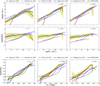Fig. 11

Dust mass (top row) and DtoG ratio (second row) as a function of the stellar mass from redshift ∼0 to 4.5, and the DtoG ratio (bottom row) as a function of metallicity at the same redshifts. Coloured solid lines represent the predictions of the semi-analytical models by Popping et al. (2017, magenta), Vijayan et al. (2019, blue), Triani et al. (2020, teal), Parente et al. (2023, cyan), and Yates et al. (2024, maroon).

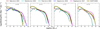Fig. 12

Dust mass function from redshift ∼0 to 3. Solid olive lines represent predictions by DUSTY-GAEA, combining the MSI and MSII runs. Coloured solid lines represent predictions from the semi-analytical models described in Fig. 11.

4.2 Limitations of our model

Estimating the gas density where dust growth and destruction occur is challenging, but essential. Popping et al. (2017) already pointed out the necessity of having a varying growth timescale as a function of the gas density for reproducing the cosmic dust evolution (i.e. simultaneously reproducing the dust mass of low- and high-redshift galaxies). This is because a short growth timescale is needed at high redshifts, which could not be achieved depending only on the (low)metallicity during those epochs. We followed their lead but adopted a different approach for estimating the gas density. Our approach uses the estimated H₂ mass (see Xie et al. 2017 for the HI-H₂ partitioning in our model) and a fixed value of H₂ volume-filling factor to estimate the volume occupied by the molecular gas (Draine 2011; see Sect. 2.2.1 for further details). The volume-filling factor is likely not the same in all galaxies at all redshifts; hence, a varying volume-filling factor would be more realistic.

Another limitation of our dust physical modelling is the lack of an explicit treatment for the grain size distribution, and associated processes of shattering and coagulation. Stellar sources mainly produce large grains (~0.1 μm), and once they are injected into the ISM, the evolution of their size distribution is shaped by destruction, growth, shattering and coagulation (Hirashita 2013). Small grains due to their large surface area favour destruction and growth. Meanwhile, large grains are more likely to shatter into smaller grains or coagulate to form larger ones (e.g. Hirashita 2013; Aoyama et al. 2020; Parente et al. 2023). Hirashita (2012) argued that the effect of coagulation on the total dust mass budget could be neglected. Indeed, our model predictions are very similar to those by Parente et al. (2023) who included a treatment of the grain size distribution based on the two-size approximation (Hirashita 2015). In future work, we plan to address this in the framework of our model, expanding it to include a treatment for grain size.

There are several channels through which dust could actively influence galaxy evolution (e.g. review by Dorschner & Henning 1995). For instance, molecular hydrogen forms most efficiently on the surfaces of dust grains (e.g. Hirashita et al. 2002; Cazaux & Tielens 2004; Wakelam et al. 2017), providing star formation with its necessary fuel (e.g. Bigiel et al. 2008; Fukui & Kawamura 2010; Schruba et al. 2011). Dust depletes a considerable amount of metals from the gas phase (e.g. Zhukovska et al. 2016; Zhukovska et al. 2018), affecting the ability of gas to cool down. Additionally, dust heats the ISM via processes such as the photoelectric heating, which is the primary heating process in the cold neutral and diffuse atomic hydrogen regions (Wolfire et al. 1995; Ingalls et al. 2002). Photoelectric heating suppresses star formation, while enhancing SNe feedback (Forbes et al. 2016; Hu et al. 2017; Osman et al. 2020). Dust also plays a role in enriching the circumgalactic medium through dusty outflows (Ferrara et al. 1991 ; Aguirre et al. 2001 ; Bianchi & Ferrara 2005; Bekki 2015; Hirashita & Aoyama 2019; Kannan et al. 2022). In short, accounting for dust influence on galaxies involves accounting for all or some of these processes. In the current version of our model, we account only for metal depletion and the enrichment of the circumgalactic medium as part of the baryon cycle; inherently, this influences the gas cooling. Future developments of the model would include some of these other processes. In particular, molecular hydrogen formation on dust grains will have an impact on the star formation rates of our simulated galaxies since our star formation recipe depends on the molecular hydrogen abundance (Xie et al. 2017).

5 Summary and conclusions

In this paper, we have presented a novel implementation of dust formation by stars, dust destruction by SNe shocks and hot gas, and growth within the dense ISM in the GAEA model. Our analysis demonstrates that the model successfully reproduces a wide range of observational constraints: the build-up of dust as a function of stellar mass out to z ~ 6, the scaling relations between the DtoG-DtoM ratio and stellar mass-metallicity in the local Universe, and the DMF out to z ~ 1.

A key finding of our study is the dominant role of dust growth in the dense ISM, which emerges as the primary contribution to the cosmic dust budget to z ~ 8. Without such efficient growth, the observed dust abundances at high redshift cannot be explained. At the same time, the model highlights the persistent difficulties in reproducing the number densities of dust-rich galaxies at z > 4. These findings align with the broader theoretical landscape, suggesting that current prescriptions for stellar yields, condensation efficiencies, or ISM conditions remain incomplete or should be improved or modified at early cosmic epochs.

In this regime, the young age of the Universe challenges efficient dust formation via the growth mechanism, and dust formation by stars is expected to dominate the dust mass budget. However, current observational constraints mostly include massive galaxies for which growth might have played a role due to the earlier formation times. Observational measurements for low-mass galaxies (M_* < 10⁹ M_⊙) at high redshifts are necessary to improve our understanding of dust production at early times.

From a theoretical perspective, our study highlights the need for refined theoretical treatments that include grain size distribution as well as metallicity-dependent condensation efficiencies. A self-consistent modelling of molecular hydrogen formation on dust grains could also help break model degeneracies and provide more robust predictions to be tested against the ever increasing amount of observational data we are gathering, particularly at early cosmic epochs.

Acknowledgements

We are grateful to G. Popping, A. Vijayan, D. Triani, M. Parente, and R. Yates for making predictions of their models available to us. We are also grateful to M. Parente, R. Yates, H. Hirashita, M. Pannella, and S. Cristiani for stimulating discussions. We acknowledge support from the INAF 2022 Theory Grant “The critical role of DUST in the cosmic barYon cycle”. OO and FF acknowledge support from the INAF 2024 RSN1 Minigrant “The effect of a variable IMF on Galaxy Evolution and Assembly: from the local to the high-z Universe”. This work has been partially supported by the Italian Ministry of University and Research (MUR) Missione 4 “Istruzione e Ricerca” -Componente C2, Investimento 1.1 Fondo per il Programma Nazionale di Ricerca e Progetti di Rilevante Interesse Nazionale (PRIN), the PRIN 2022 PNRR grant under the National Recovery and Resilience Plan (PNRR): project P2022ZLW4T “Next-generation computing and data technologies to probe the cosmic metal content”. L.X. acknowledges support from the National Natural Science Foundation of China (grant number 12041302), the Ministry of Science and Technology of China (grant No. 2020SKA0110100).

References

Aguirre, A., Hernquist, L., Katz, N., Gardner, J., & Weinberg, D. 2001, ApJ, 556, L11 [Google Scholar]
Algera, H. S. B., Rowland, L., Stefanon, M., et al. 2026, MNRAS, 545, 22 [Google Scholar]
Andersen, M., Rho, J., Reach, W. T., Hewitt, J. W., & Bernard, J. P. 2011, ApJ, 742, 7 [Google Scholar]
Aoyama, S., Hou, K., Shimizu, I., et al. 2017, MNRAS, 466, 105 [NASA ADS] [CrossRef] [Google Scholar]
Aoyama, S., Hou, K., Hirashita, H., Nagamine, K., & Shimizu, I. 2018, MNRAS, 478, 4905 [NASA ADS] [CrossRef] [Google Scholar]
Aoyama, S., Hirashita, H., & Nagamine, K. 2020, MNRAS, 491, 3844 [NASA ADS] [Google Scholar]
Asano, R. S., Takeuchi, T. T., Hirashita, H., & Inoue, A. K. 2013a, Earth Planets Space, 65, 213 [NASA ADS] [CrossRef] [Google Scholar]
Asano, R. S., Takeuchi, T. T., Hirashita, H., & Nozawa, T. 2013b, MNRAS, 432, 637 [NASA ADS] [CrossRef] [Google Scholar]
Bakes, E. L. O., & Tielens, A. G. G. M. 1994, ApJ, 427, 822 [NASA ADS] [CrossRef] [Google Scholar]
Barlow, M. J. 1978, MNRAS, 183, 367 [NASA ADS] [CrossRef] [Google Scholar]
Beeston, R. A., Wright, A. H., Maddox, S., et al. 2018, MNRAS, 479, 1077 [NASA ADS] [Google Scholar]
Beeston, R. A., Gomez, H. L., Dunne, L., et al. 2024, MNRAS, 535, 3162 [Google Scholar]
Bekki, K. 2013, MNRAS, 432, 2298 [Google Scholar]
Bekki, K. 2015, MNRAS, 449, 1625 [Google Scholar]
Bennett, C. L., Larson, D., Weiland, J. L., et al. 2013, ApJS, 208, 20 [Google Scholar]
Berta, S., Lagache, G., Beelen, A., et al. 2025, A&A, 696, A193 [NASA ADS] [CrossRef] [EDP Sciences] [Google Scholar]
Bertoldi, F., Carilli, C. L., Cox, P., et al. 2003, A&A, 406, L55 [NASA ADS] [CrossRef] [EDP Sciences] [Google Scholar]
Bianchi, S., & Ferrara, A. 2005, MNRAS, 358, 379 [NASA ADS] [CrossRef] [Google Scholar]
Bianchi, S., & Schneider, R. 2007, MNRAS, 378, 973 [NASA ADS] [CrossRef] [Google Scholar]
Bianchi, S., De Vis, P., Viaene, S., et al. 2018, A&A, 620, A112 [NASA ADS] [CrossRef] [EDP Sciences] [Google Scholar]
Bigiel, F., Leroy, A., Walter, F., et al. 2008, AJ, 136, 2846 [NASA ADS] [CrossRef] [Google Scholar]
Black, J. H. 1987, Astrophys. Space Sci. Lib., 134, 731 [Google Scholar]
Bocchio, M., Marassi, S., Schneider, R., et al. 2016, A&A, 587, A157 [NASA ADS] [CrossRef] [EDP Sciences] [Google Scholar]
Boylan-Kolchin, M., Springel, V., White, S. D. M., et al. 2009, MNRAS, 398, 1150 [NASA ADS] [CrossRef] [Google Scholar]
Calura, F., Pipino, A., & Matteucci, F. 2008, A&A, 479, 669 [NASA ADS] [CrossRef] [EDP Sciences] [Google Scholar]
Cantarella, S., De Lucia, G., Fontanot, F., et al. 2025, A&A, submitted [arXiv:2511.03787] [Google Scholar]
Casey, C. M. 2012, MNRAS, 425, 3094 [Google Scholar]
Cazaux, S., & Tielens, A. G. G. M. 2004, ApJ, 604, 222 [NASA ADS] [CrossRef] [Google Scholar]
Chabrier, G. 2003, PASP, 115, 763 [Google Scholar]
Chieffi, A., & Limongi, M. 2004, ApJ, 608, 405 [NASA ADS] [CrossRef] [Google Scholar]
Clark, C. J. R., Dunne, L., Gomez, H. L., et al. 2015, MNRAS, 452, 397 [NASA ADS] [CrossRef] [Google Scholar]
Clemens, M. S., Negrello, M., De Zotti, G. J., et al. 2013, MNRAS, 433, 695 [NASA ADS] [CrossRef] [Google Scholar]
Corbelli, E., Bianchi, S., Cortese, L., et al. 2012, A&A, 542, A32 [NASA ADS] [CrossRef] [EDP Sciences] [Google Scholar]
Cortese, L., Ciesla, L., Boselli, A., et al. 2012, A&A, 540, A52 [NASA ADS] [CrossRef] [EDP Sciences] [Google Scholar]
Croton, D. J., Springel, V., & White, S. D. M. 2006, MNRAS, 365, 11 [NASA ADS] [CrossRef] [Google Scholar]
da Cunha, E., Eminian, C., Charlot, S., & Blaizot, J. 2010, MNRAS, 403, 1894 [Google Scholar]
da Cunha, E., Walter, F., Smail, I. R., et al. 2015, ApJ, 806, 110 [Google Scholar]
Dayal, P., Ferrara, A., Sommovigo, L., et al. 2022, MNRAS, 512, 989 [NASA ADS] [CrossRef] [Google Scholar]
De Cia, A., Ledoux, C., Savaglio, S., et al. 2013, A&A, 560, A88 [NASA ADS] [CrossRef] [EDP Sciences] [Google Scholar]
De Cia, A., Ledoux, C., Mattsson, L., et al. 2016, A&A, 596, A97 [NASA ADS] [CrossRef] [EDP Sciences] [Google Scholar]
De Lucia, G., & Blaizot, J. 2007, MNRAS, 375, 2 [Google Scholar]
De Lucia, G., Boylan-Kolchin, M., Benson, A. J., Fontanot, F., & Monaco, P. 2010, MNRAS, 406, 1533 [NASA ADS] [Google Scholar]
De Lucia, G., Tornatore, L., Frenk, C. S., et al. 2014, MNRAS, 445, 970 [Google Scholar]
De Lucia, G., Fontanot, F., Xie, L., & Hirschmann, H. 2024, A&A, 687, A68 [NASA ADS] [CrossRef] [EDP Sciences] [Google Scholar]
De Vis, P., Jones, A., Viaene, S., et al. 2019, A&A, 623, A5 [NASA ADS] [CrossRef] [EDP Sciences] [Google Scholar]
Demyk, K. 2011, EPJ Web Conf., 18, 03001 [NASA ADS] [CrossRef] [EDP Sciences] [Google Scholar]
Dorschner, J., & Henning, T. 1995, ARA&A, 6, 271 [Google Scholar]
Draine, B. T. 1978, ApJSS, 36, 595 [Google Scholar]
Draine, B. T. 2003, ARA&A, 41, 241 [Google Scholar]
Draine, B. T. 2007, ApJ, 663, 894 [Google Scholar]
Draine, B. T. 2011, Physics of the Interstellar and Intergalactic Medium, ed. B. T. Draine (Princeton: Princeton University Press) [Google Scholar]
Draine, B. T., Dale, D. A., Bendo, G., et al. 2007, ApJ, 663, 866 [NASA ADS] [CrossRef] [Google Scholar]
Duley, W. W., & Millar, T. J. 1978, ApJ, 220, 124 [Google Scholar]
Dulieu, F., Congiu, E., Noble, J., et al. 2013, Sci. Rep., 3, 1338 [Google Scholar]
Dunne, L., Eales, S. A., & Edmunds, M. G. 2003, MNRAS, 341, 589 [NASA ADS] [CrossRef] [Google Scholar]
Dunne, L., Gomez, H. L., da Cunha, E., et al. 2011, MNRAS, 417, 1510 [NASA ADS] [CrossRef] [Google Scholar]
Dwek, E. 1998, ApJ, 501, 643 [NASA ADS] [CrossRef] [Google Scholar]
Dwek, E., & Scalo, J. M. 1980, ApJ, 239, 193 [NASA ADS] [CrossRef] [Google Scholar]
Eales, S., Chapin, E. L., Devlin, M. J., et al. 2009, ApJ, 707, 1779 [Google Scholar]
Faisst, A. L., Liu, L.-J., Dubois, Y., et al. 2025, ApJ, submitted [arXiv:2510.16106] [Google Scholar]
Ferrara, A., Ferrini, F., Barsella, B., & Franco, J. 1991, ApJ, 381, 137 [Google Scholar]
Ferrarotti, A. D., & Gail, H. P. 2006, A&A, 553, 576 [Google Scholar]
Fontanot, F., De Lucia, G., Hirschmann, H., et al. 2020, MNRAS, 496, 3943 [CrossRef] [Google Scholar]
Fontanot, F., Calabrò, A., Talia, M., et al. 2021, MNRAS, 504, 4481 [CrossRef] [Google Scholar]
Fontanot, F., La Barbera, F., De Lucia, G., et al. 2024, A&A, 686, A302 [NASA ADS] [CrossRef] [EDP Sciences] [Google Scholar]
Fontanot, F., De Lucia, G., Xie, L., et al. 2025, A&A, 699, A108 [NASA ADS] [CrossRef] [EDP Sciences] [Google Scholar]
Forbes, J. C., Krumholz, M. R., Goldbaum, N. J., & Dekel, A. 2016, Nature, 535, 523 [Google Scholar]
Fukui, Y., & Kawamura, A. 2010, ARA&A, 48, 547 [Google Scholar]
Galametz, M., Madden, S. C., Galliano, F., et al. 2011, A&A, 532, A56 [NASA ADS] [CrossRef] [EDP Sciences] [Google Scholar]
Galliano, F., Galametz, M., & Jones, A. P. 2018, ARA&A, 56, 673 [Google Scholar]
Ginolfi, M., Graziani, L., Schneider, R., et al. 2018, MNRAS, 473, 4538 [NASA ADS] [CrossRef] [Google Scholar]
Gioannini, L., Matteucci, F., Vladilo, G., & Calura, F. 2017, MNRAS, 464, 985 [CrossRef] [Google Scholar]
Gjergo, E., Granato, G. L., Murante, G., et al. 2018, MNRAS, 479, 2588 [NASA ADS] [CrossRef] [Google Scholar]
Glover, S. C. O., & Clark, P. C. 2012, MNRAS, 421, 9 [NASA ADS] [Google Scholar]
Granato, G. L., Ragone-Figueroa, C., Taverna, A., et al. 2021, MNRAS, 503, 511 [NASA ADS] [CrossRef] [Google Scholar]
Grossi, M., Hunt, L. K., Madden, S. C., et al. 2015, A&A, 574, A126 [NASA ADS] [CrossRef] [EDP Sciences] [Google Scholar]
Groves, B. A., Dopita, M. A., & Sutherland, R. S. 2004, ApJS, 153, 75 [NASA ADS] [CrossRef] [Google Scholar]
Guo, Q., White, S., Angulo, R. E., et al. 2013, MNRAS, 428, 1351 [NASA ADS] [CrossRef] [Google Scholar]
Gutkin, J., Charlot, S., & Bruzual, G. 2016, MNRAS, 462, 1757 [Google Scholar]
Hill, A. S., Mac Low, M.-M., Gatto, A., & Ibanez-Mejia, J. C. 2018, ApJ, 861, 55 [Google Scholar]
Hirashita, H. 1999, ApJ, 510, L99 [NASA ADS] [CrossRef] [Google Scholar]
Hirashita, H. 2012, MNRAS, 422, 1263 [NASA ADS] [CrossRef] [Google Scholar]
Hirashita, H. 2013, Proceedings of The Life Cycle of Dust in the Universe: Observations, Theory, and Laboratory Experiments (LCDU2013), 27, Available at: http://pos.sissa.it/cgi-bin/reader/conf.cgi?confid=207 [Google Scholar]
Hirashita, H. 2015, MNRAS, 447, 2937 [NASA ADS] [CrossRef] [Google Scholar]
Hirashita, H., & Aoyama, S. 2019, MNRAS, 482, 2555 [NASA ADS] [CrossRef] [Google Scholar]
Hirashita, H., & Kuo, T. 2011, MNRAS, 416, 1340 [NASA ADS] [CrossRef] [Google Scholar]
Hirashita, H., Tajiri, Y. Y., & Kamaya, H. 2002, A&A, 388, 439 [NASA ADS] [CrossRef] [EDP Sciences] [Google Scholar]
Hirschmann, M., De Lucia, G., & Fontanot, F. 2016, MNRAS, 461, 1760 [Google Scholar]
Hirschmann, M., Charlot, S., & Somerville, R. S. 2023, MNRAS, 526, 3504 [NASA ADS] [CrossRef] [Google Scholar]
Hou, K., Hirashita, H., Nagamine, K., Aoyama, S., & Shimizu, I. 2017, MNRAS, 469, 870 [NASA ADS] [CrossRef] [Google Scholar]
Hou, K.-C., Aoyama, S., Hirashita, H., Nagamine, K., & Shimizu, I. 2019, MNRAS, 485, 1727 [NASA ADS] [CrossRef] [Google Scholar]
Hu, C.-Y., Naab, T., Glover, S. C. O., Walch, S., & Clark, P. C. 2017, MNRAS, 471, 2151 [NASA ADS] [CrossRef] [Google Scholar]
Ingalls, J. G., Reach, W. T., & Bania, T. M. 2002, ApJ, 579, 289 [NASA ADS] [CrossRef] [Google Scholar]
Inoue, A. K. 2003, PASJ, 55, 901 [NASA ADS] [CrossRef] [Google Scholar]
Issa, M. R., MacLaren, I., & Wolfendale, A. W. 1990, A&A, 236, 237 [NASA ADS] [Google Scholar]
James, A., Dunne, L., Eales, S., & Edmunds, M. G. 2002, MNRAS, 335, 753 [CrossRef] [Google Scholar]
Jones, A. P. 2004, ASP Conf. Ser., 309, 347 [NASA ADS] [Google Scholar]
Jones, A. P., & Williams, D. A. 1985, MNRAS, 217, 413 [NASA ADS] [Google Scholar]
Jones, A. P., Tielens, A. G. G. M., Hollenbach, D. J., & McKee, C. F. 1994, ApJ, 433, 797 [NASA ADS] [CrossRef] [Google Scholar]
Kannan, R., Smith, A., Garaldi, E., et al. 2022, MNRAS, 514, 3857 [CrossRef] [Google Scholar]
Karakas, A. I. 2010, MNRAS, 403, 1413 [NASA ADS] [CrossRef] [Google Scholar]
Kewley, L. J., & Ellison, S. L. 2008, ApJ, 681, 1183 [Google Scholar]
Klessen, R. S., & Glover, S. C. O. 2016, Star Formation in Galaxy Evolution: Connecting Numerical Models to Reality, Saas-Fee Advanced Course (Berlin: Springer), 43, 85 [Google Scholar]
Kuo, T.-M., & Hirashita, H. 2012, MNRAS, 424, L34 [NASA ADS] [CrossRef] [Google Scholar]
Li, Q., Narayanan, D., & Dave, R. 2019, MNRAS, 490, 1425 [CrossRef] [Google Scholar]
Lisenfeld, U., & Ferrara, A. 1998, ApJ, 496, 145 [NASA ADS] [CrossRef] [Google Scholar]
Madau, P., & Dickinson, M. 2014, ARA&A, 52, 415 [Google Scholar]
Magrini, L., Bianchi, S., Corbelli, E., et al. 2011, A&A, 535, A13 [NASA ADS] [CrossRef] [EDP Sciences] [Google Scholar]
Mathis, J. S., Rumpl, W., & Nordsieck, K. H. 1977, ApJ, 217, 425 [Google Scholar]
Mattsson, L. 2011, MNRAS, 414, 781 [Google Scholar]
McKee, C. 1989, Proc. IAU Symp., 135, 431 [Google Scholar]
McKinnon, R., Torrey, P., & Vogelsberger, M. 2016, MNRAS, 457, 3775 [CrossRef] [Google Scholar]
McKinnon, R., Torrey, P., Vogelsberger, M., Hayward, C. C., & Marinacci, F. 2017, MNRAS, 468, 1505 [NASA ADS] [CrossRef] [Google Scholar]
McKinnon, R., Torrey, P., & Vogelsberger, M. 2018, MNRAS, 478, 2851 [NASA ADS] [CrossRef] [Google Scholar]
Micelotta, E. R., Matsuura, M., & Sarangi, A. 2018, Space Sci. Rev., 214, 58 [Google Scholar]
Murray, N., & Rahman, M. 2010, ApJ, 709, 424 [NASA ADS] [CrossRef] [Google Scholar]
Nanni, A., Romano, M., Donevski, D., et al. 2025, ApJ, 988, 8 [Google Scholar]
Nersesian, A., Xilouris, E. M., Bianchi, S., et al. 2019, A&A, 624, A80 [NASA ADS] [CrossRef] [EDP Sciences] [Google Scholar]
Nozawa, T., Kozasa, T., Umeda, H., Maeda, K., & Nomoto, K. 2003, ApJ, 598, 785 [NASA ADS] [CrossRef] [Google Scholar]
Nozawa, T., Kozasa, T., & Habe, A. 2006, ApJ, 648, 435 [NASA ADS] [CrossRef] [Google Scholar]
Osman, O., Bekki, K., & Cortese, L. 2020, MNRAS, 498, 2075 [Google Scholar]
Parente, M., Ragone-Figueroa, C., Granato, G. L., et al. 2022, MNRAS, 515, 2053 [NASA ADS] [CrossRef] [Google Scholar]
Parente, P., Ragone-Figueroa, C., Granato, G. L., et al. 2023, MNRAS, 521, 6105 [NASA ADS] [CrossRef] [Google Scholar]
Planck Collaboration XIII. 2016, A&A, 594, A13 [NASA ADS] [CrossRef] [EDP Sciences] [Google Scholar]
Popping, G., & Péroux, C. 2022, MNRAS, 513, 1531 [CrossRef] [Google Scholar]
Popping, G., Somerville, R. S., & Galametz, M. 2017, MNRAS, 471, 3152 [NASA ADS] [CrossRef] [Google Scholar]
Pozzi, F., Calura, F., Zamorani, G., et al. 2020, MNRAS, 491, 5073 [NASA ADS] [CrossRef] [Google Scholar]
Péroux, C., & Howk, J. C. 2020, ARA&A, 58, 363 [Google Scholar]
Relaño, M., De Looze, I., Kennicutt, R. C., et al. 2018, A&A, 613, A43 [NASA ADS] [CrossRef] [EDP Sciences] [Google Scholar]
Rémy-Ruyer, A., Madden, S. C., Galliano, F., et al. 2014, A&A, 563, A31 [Google Scholar]
Rémy-Ruyer, A., Madden, S. C., Galliano, F., et al. 2015, A&A, 582, A121 [Google Scholar]
Riechers, D. A., Carilli, C. L., Capak, P. L., et al. 2014, ApJ, 796, 84 [Google Scholar]
Rowlands, K., Dunne, L., Dye, S., et al. 2014, MNRAS, 441, 1017 [NASA ADS] [CrossRef] [Google Scholar]
Santini, P., Maiolino, R., Magnelli, B., et al. 2014, A&A, 562, A30 [NASA ADS] [CrossRef] [EDP Sciences] [Google Scholar]
Sarangi, A., Matsuura, M., & Micelotta, E. R. 2018, Space Sci. Rev., 214, 48 [Google Scholar]
Sargent, B. A., Srinivasan, S., Meixner, M., et al. 2010, ApJ, 716, 878 [NASA ADS] [CrossRef] [Google Scholar]
Savage, B. D., & Sembach, K. R. 1996, ARA&A, 34, 279 [Google Scholar]
Schruba, A., Leroy, A., Walter, F., et al. 2011, AJ, 142, 37 [NASA ADS] [CrossRef] [Google Scholar]
Shivaei, I., Alberts, S., Florian, M., et al. 2024, A&A, 690, A89 [NASA ADS] [CrossRef] [EDP Sciences] [Google Scholar]
Smith, D. J. B., Dunne, L., da Cunha, E., et al. 2012, MNRAS, 427, 703 [Google Scholar]
Sparre, M., Hartoog, O. E., Krühler, T., et al. 2014, ApJ, 785, 150 [NASA ADS] [CrossRef] [Google Scholar]
Springel, V., White, S. D. M., Jenkins, A., et al. 2005, Nature, 435, 629 [Google Scholar]
Srinivasan, S., Sargent, B. A., Matsuura, M., et al. 2010, A&A, 524, A49 [NASA ADS] [CrossRef] [EDP Sciences] [Google Scholar]
Thielemann, F. K. 2003, in From Twilight to Highlight: the Physics of Supernovae Supernova Nucle- osynthesis and Galactic Evolution, eds. W. Hillebrandt, & B. Leibundgut (Berlin: Springer-Verlag), 331 [Google Scholar]
Traina, A., Magnelli, B., Gruppioni, C., et al. 2024, A&A, 690, A84 [NASA ADS] [CrossRef] [EDP Sciences] [Google Scholar]
Triani, D. P., Sinha, M., Croton, D. J., Pacifici, C., & Dwek, E. 2020, MNRAS, 493, 2490 [NASA ADS] [CrossRef] [Google Scholar]
Tsai, J. C., & Mathews, W. G. 1995, ApJ, 448, 84 [CrossRef] [Google Scholar]
Valiante, R., Schneider, R., Bianchi, S., & Andersen, A. C. 2009, MNRAS, 397, 1661 [CrossRef] [Google Scholar]
Ventura, P., di Criscienzo, M., Schneider, R., et al. 2012, MNRAS, 420, 1442 [Google Scholar]
Vijayan, A. P., Clay, S. J., Thomas, P. A., et al. 2019, MNRAS, 489, 4072 [NASA ADS] [CrossRef] [Google Scholar]
Vlahakis, C., Dunne, L., & Eales, S. 2005, MNRAS, 364, 1253 [NASA ADS] [CrossRef] [Google Scholar]
Wakelam, V., Bron, E., Cazaux, S., et al. 2017, Mol. Astrophys., 9, 1 [Google Scholar]
Wang, J., De Lucia, G., Kitzbichler, M. G., & White, S. D. M. 2008, MNRAS, 384, 1301 [CrossRef] [Google Scholar]
Watson, W. D. 1972, ApJ, 176, 103 [Google Scholar]
Watson, D., Christensen, L., Knudsen, K. K., Richard, J., & et al. 2015, Nature, 519, 327 [Google Scholar]
Weingartner, J. C., & Draine, B. T. 2001, ApJS, 134, 263 [CrossRef] [Google Scholar]
Whittet, D. 1989, IAU Symp., 135, 455 [Google Scholar]
Williams, D. A. 1987, IAU Symp., 537, 538 [Google Scholar]
Wiseman, P., Schady, P., Bolmer, J., et al. 2017, A&A, 599, A24 [NASA ADS] [CrossRef] [EDP Sciences] [Google Scholar]
Wolfire, M. G., Hollenbach, D., McKee, C. F., Tielens, A. G. G. M., & Bakes, E. O. 1995, ApJ, 443, 152 [NASA ADS] [CrossRef] [Google Scholar]
Wolfire, M. G., Mckee, C. F., & Tielens, A. G. G. M. 2003, ApJ, 587, 278 [CrossRef] [Google Scholar]
Xie, L., De Lucia, G., Hirschmann, M., et al. 2017, MNRAS, 469, 968 [Google Scholar]
Xie, L., De Lucia, G., Hirschmann, M., & Fontanot, F. 2020, MNRAS, 498, 4327 [NASA ADS] [CrossRef] [Google Scholar]
Yamasawa, D., Habe, A., Kozasa, T., et al. 2011, ApJ, 734, 44 [Google Scholar]
Yates, R. M., Hendriks, D., Vijayan, A. P., et al. 2024, MNRAS, 527, 6292 [Google Scholar]
Zafar, T., & Watson, D. 2013, A&A, 560, A26 [NASA ADS] [CrossRef] [EDP Sciences] [Google Scholar]
Zhukovska, S., Gail, H.-P., & Trieloff, M. 2008, A&A, 479, 453 [NASA ADS] [CrossRef] [EDP Sciences] [Google Scholar]
Zhukovska, S., Dobbs, C., Jenkins, E. B., & Klessen, R. S. 2016, ApJ, 831, 147 [NASA ADS] [CrossRef] [Google Scholar]
Zhukovska, S., Henning, T., & Dobbs, C. 2018, ApJ, 857, 94 [Google Scholar]

https://sites.google.com/inaf.it/gaea/home

The choice of the IMF affects the chemical enrichment at fixed yields since it alters the relative number of AGB stars, SNIa, and SNII. The reference model (GAEA) also includes a variant that allows for variable IMF prescriptions (see e.g. Fontanot et al. 2024). However, in this work, we focus on the standard choice of a Universal MilkyWay-like IMF. We will address the effects of varying the IMF on dust abundance at high redshift in our future works.

The single SN destruction efficiency, ζ_SN, we adopted is consistent with this limit. The destruction efficiency increases quadratically with the ambient gas density according to Nozawa et al. (2006) model (see their Fig. 10 and Eq. (A3)).

⁴

Throughout the text, we present predictions of the dust properties in the cold gas reservoir, representing the ISM in modelled galaxies.

⁵

We limit ourselves to a comparison with semi-analytical models because of the use of the same theoretical framework makes the comparison more straightforward. We compare our DMF predictions with predictions from hydrodynamical simulations in Appendix C.

Appendix A Dust destruction models

There are two different approaches that can be found in literature for estimating the destruction timescale. These employ the concepts of the mass of the ISM completely cleared of dust by SN shocks (Valiante et al. 2009; Popping et al. 2017; Vijayan et al. 2019) and the mass of the ISM swept up by the shocks (McKee 1989; Dwek 1998; McKinnon et al. 2016; Aoyama et al. 2017; Li et al. 2019). In Sect. 2.2 we present the model we used in most of our analysis, which is a flavor of the second approach. In this section we present two extra models, employing flavors of the two approaches.

A.1 Destruction timescales

The destruction timescale for the first model adopting the first approach is given by the following equation: $τ_{d e s} = \begin{array}{rcl} \frac{M_{H I + H I I}}{M_{c l e a r e d} γ_{S N} ξ_{S N}} & y r \end{array},$ $Mathematical equation: \tau_{des} = \begin{array}{rcl} \frac{M_{HI+HII}}{M_{cleared} \gamma_{SN} \xi_{SN}} & yr \end{array},$ (A.1)

where M_HI+HII is the mass of the atomic and ionised gas, M_cleared is the mass of the ISM cleared of dust, γ_SN is SNe rate, and ξ_SN is the fraction of clustered SNe. We adopt values of M_cleared = 980 for silicates and 600 for carbon dust (Popping et al. 2017).

For the second model adopting the second approach, the destruction timescale is given by the following equation (same as Eq. 10): $τ_{d e s} = \begin{array}{rcl} \frac{M_{H I + H I I}}{M_{s w e p t} γ_{S N} ξ_{S N} ζ_{S N}} & y r \end{array},$ $Mathematical equation: \tau_{des} = \begin{array}{rcl} \frac{M_{HI+HII}}{M_{swept} \gamma_{SN} \xi_{SN} \zeta_{SN}} & yr \end{array},$ (A.2)

where M_swept is the mass of the ISM swept up, and ζ_SN is SNe destruction efficiency. For this model, we adopted the functional form by Yamasawa et al. (2011) for M_swept and the same parameter values as in our fiducial model. $M_{s w e p t} = \begin{array}{rcl} 1535 (n_{0})^{- 0.202} [(\frac{Z}{Z_{⊙}}) + 0.039]^{- 0.298} & M_{⊙} \end{array},$ $Mathematical equation: M_{swept} = \begin{array}{rcl} 1535(n_0)^{-0.202}[(\frac{Z}{Z_\odot}) + 0.039]^{-0.298} & M_{\odot} \end{array},$ (A.3)

where Z is the gas metallicity. This is a fitting formula, and it is accurate within less than 16% for n₀ between 0.03 and 30 cm⁻³, and $\frac{Z}{Z_{⊙}}$ $Mathematical equation: $\frac{Z}{Z_\odot}$$ between 10⁻⁴ and 1.

A.2 Dust mass-stellar mass relation

For these test models, we only run the model using the MSI merger trees. Figure A.1 shows predictions of the dust mass as a function of the stellar mass from z ~ 0 to 5.5 in the two models presented here, together with the fiducial model. Olive, magenta and orange lines and shaded areas represent predictions of the fiducial, the model adopting the first approach, and the model adopting the second modified approach, respectively. In the mass range resolved by the MSI merger trees, predictions of the three models are practically identical, which we attribute to the efficient growth in this mass range, making the results insensitive to the changes we implement in the destruction model. The situation could be different at low stellar masses. We will address the destruction efficiency in the low mass range together with variations in the condensation efficiency in stellar ejecta in future works.

Appendix B Dust formation and destruction rates

Fig. B.1 presents the dust formation rates by stars (solid-dashed), destruction by SNe forward shocks (solid) and growth in the dense ISM (dashed-dotted) in the model variant DUSTY-GAEA-Dwek. As discussed in Fig. 3, the rates presented here behave similarly to the rates in the model variant DUSTY-GAEA. Besides the slightly steeper correlation between the dust growth rate and stellar mass in the DUSTY-GAEA-Dwek model, this model variant also has a larger scatter compared to the DUSTY-GAEA variant.

Appendix C The dust mass function in hydrodynamical simulations

In this appendix we compare our fiducial model predictions of the DMF to predictions from the hydrodynamical simulations by McKinnon et al. (2017), Aoyama et al. (2018), Hou et al. (2019), Li et al. (2019), and Parente et al. (2022) in Fig. C.1. All these simulations explicitly model dust formation and evolution, where they include formation by stars, destruction by SNe and sputtering in the hot gas, and growth in the dense ISM. Simulations by Aoyama et al. (2018), Hou et al. (2019), and Parente et al. (2022) also include shattering and coagulation of dust grains. These latter models employ the same dust growth and destruction models as those described in Hirashita & Kuo (2011) and the formulae developed by Aoyama et al. (2017), respectively. Meanwhile, McKinnon et al. (2017) and Li et al. (2019) adopted the classic prescriptions by Dwek (1998) and McKee (1989), respectively. Each of these simulations adopted slightly different prescriptions for dust formation by stars. For further details, we refer the reader to the original papers. Note that the biggest volume simulated by these simulations is 100 cMpc by Li et al. (2019).

In the local Universe, our model predicts a higher number density than all models at the low dust mass end (< 10⁶ M_⊙), while at the high mass end (> 10^8.5 M_⊙), our model predictions are only higher than predictions by McKinnon et al. and Parente et al. In the intermediate mass range, our predictions are broadly consistent with all but the simulation by Aoyama et al. Similar trends are seen in predictions beyond the local Universe, where our model dominates the low mass end and some of the other models dominate the high mass end. The behaviour of these simulations is quite diverse, and only simulations by McKinnon et al., Li et al., and Parente et al. reproduce well the observational constraints in the local Universe. Aoyama et al. attributed their high number density at the high dust mass end to inefficient feedback at the high end of the stellar mass range, while Hou et al. argued that the inconsistency with observations is due to dust overproduction.

Fig. A.1

Dust mass as a function of the stellar mass at different redshifts. Olive (DUSTY refers to the model DUSTY-GAEA), magenta and orange lines and shaded areas represent predictions of the fiducial, the model adopting the first approach, and the model adopting the second modified approach, respectively. Shaded areas represent the 16th-84th percentile region.

Fig. B.1

Dust formation, destruction, and growth rates as predicted by the DUSTY-GAEA-Dwek model. The solid-dashed, solid and dashed-dotted lines represent the dust formation rates by stars, destruction by SNe forward shocks, and growth in the dense ISM, respectively. Shaded areas represent the 16th-84th percentile region.

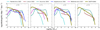Fig. C.1

The DMF from redshift ~ 0 to 3. Solid olive lines represent predictions by DUSTY-GAEA, combining the MSI and MSII runs. Coloured solid lines represent predictions from the hydrodynamical simulations by McKinnon et al. (2017, magenta), Aoyama et al. (2018, blue), Hou et al. (2019, teal), Li et al. (2019, maroon), and Parente et al. (2022, cyan).

All Tables

Table 1

Parameter values for the dust growth model based on the Zhukovska et al. (2008) model.

In the text

Table 2

Main characteristics of the dust models presented in this work.

In the text

Table 3

Dust physics prescriptions adopted in the semi-analytical models considered in this work for comparison with our predictions.

In the text

All Figures

	Fig. 1 Normalised histograms of the estimated density of the warm intercloud medium (top) and cold molecular gas (bottom) from z ∼ 0 to z ∼ 5.5. Predictions are based on the MSI merger trees. We limited the distributions to resolved galaxies (see Sect. 3 for details).
In the text

	Fig. 9 Predictions of the CDD as a function of the lookback time (bottom x-axis) and redshift (top x-axis). Solid, dashed, and dashed-dotted lines represent predictions by DUSTY-GAEA, DUSTY-GAEA-Dwek, and DUSTY-GAEA-NoG models, respectively. Grey diamonds represent data collected by Berta et al. (2025), while the red dots represent their measurements.
In the text

	Fig. 10 Predictions of the CDD formation and destruction rates. Line styles have the same meaning as in Fig. 3.
In the text

Fig. 11

In the text

	Fig. 12 Dust mass function from redshift ∼0 to 3. Solid olive lines represent predictions by DUSTY-GAEA, combining the MSI and MSII runs. Coloured solid lines represent predictions from the semi-analytical models described in Fig. 11.
In the text

	Fig. A.1 Dust mass as a function of the stellar mass at different redshifts. Olive (DUSTY refers to the model DUSTY-GAEA), magenta and orange lines and shaded areas represent predictions of the fiducial, the model adopting the first approach, and the model adopting the second modified approach, respectively. Shaded areas represent the 16th-84th percentile region.
In the text

	Fig. B.1 Dust formation, destruction, and growth rates as predicted by the DUSTY-GAEA-Dwek model. The solid-dashed, solid and dashed-dotted lines represent the dust formation rates by stars, destruction by SNe forward shocks, and growth in the dense ISM, respectively. Shaded areas represent the 16th-84th percentile region.
In the text

	Fig. C.1 The DMF from redshift ~ 0 to 3. Solid olive lines represent predictions by DUSTY-GAEA, combining the MSI and MSII runs. Coloured solid lines represent predictions from the hydrodynamical simulations by McKinnon et al. (2017, magenta), Aoyama et al. (2018, blue), Hou et al. (2019, teal), Li et al. (2019, maroon), and Parente et al. (2022, cyan).
In the text

Current usage metrics show cumulative count of Article Views (full-text article views including HTML views, PDF and ePub downloads, according to the available data) and Abstracts Views on Vision4Press platform.

Data correspond to usage on the plateform after 2015. The current usage metrics is available 48-96 hours after online publication and is updated daily on week days.

Initial download of the metrics may take a while.

[R1] Aguirre, A., Hernquist, L., Katz, N., Gardner, J., & Weinberg, D. 2001, ApJ, 556, L11 [Google Scholar]

[R2] Algera, H. S. B., Rowland, L., Stefanon, M., et al. 2026, MNRAS, 545, 22 [Google Scholar]

[R3] Andersen, M., Rho, J., Reach, W. T., Hewitt, J. W., & Bernard, J. P. 2011, ApJ, 742, 7 [Google Scholar]

[R4] Aoyama, S., Hou, K., Shimizu, I., et al. 2017, MNRAS, 466, 105 [NASA ADS] [CrossRef] [Google Scholar]

[R5] Aoyama, S., Hou, K., Hirashita, H., Nagamine, K., & Shimizu, I. 2018, MNRAS, 478, 4905 [NASA ADS] [CrossRef] [Google Scholar]

[R6] Aoyama, S., Hirashita, H., & Nagamine, K. 2020, MNRAS, 491, 3844 [NASA ADS] [Google Scholar]

[R7] Asano, R. S., Takeuchi, T. T., Hirashita, H., & Inoue, A. K. 2013a, Earth Planets Space, 65, 213 [NASA ADS] [CrossRef] [Google Scholar]

[R8] Asano, R. S., Takeuchi, T. T., Hirashita, H., & Nozawa, T. 2013b, MNRAS, 432, 637 [NASA ADS] [CrossRef] [Google Scholar]

[R9] Bakes, E. L. O., & Tielens, A. G. G. M. 1994, ApJ, 427, 822 [NASA ADS] [CrossRef] [Google Scholar]

[R10] Barlow, M. J. 1978, MNRAS, 183, 367 [NASA ADS] [CrossRef] [Google Scholar]

[R11] Beeston, R. A., Wright, A. H., Maddox, S., et al. 2018, MNRAS, 479, 1077 [NASA ADS] [Google Scholar]

[R12] Beeston, R. A., Gomez, H. L., Dunne, L., et al. 2024, MNRAS, 535, 3162 [Google Scholar]

[R13] Bekki, K. 2013, MNRAS, 432, 2298 [Google Scholar]

[R14] Bekki, K. 2015, MNRAS, 449, 1625 [Google Scholar]

[R15] Bennett, C. L., Larson, D., Weiland, J. L., et al. 2013, ApJS, 208, 20 [Google Scholar]

[R16] Berta, S., Lagache, G., Beelen, A., et al. 2025, A&A, 696, A193 [NASA ADS] [CrossRef] [EDP Sciences] [Google Scholar]

[R17] Bertoldi, F., Carilli, C. L., Cox, P., et al. 2003, A&A, 406, L55 [NASA ADS] [CrossRef] [EDP Sciences] [Google Scholar]

[R18] Bianchi, S., & Ferrara, A. 2005, MNRAS, 358, 379 [NASA ADS] [CrossRef] [Google Scholar]

[R19] Bianchi, S., & Schneider, R. 2007, MNRAS, 378, 973 [NASA ADS] [CrossRef] [Google Scholar]

[R20] Bianchi, S., De Vis, P., Viaene, S., et al. 2018, A&A, 620, A112 [NASA ADS] [CrossRef] [EDP Sciences] [Google Scholar]

[R21] Bigiel, F., Leroy, A., Walter, F., et al. 2008, AJ, 136, 2846 [NASA ADS] [CrossRef] [Google Scholar]

[R22] Black, J. H. 1987, Astrophys. Space Sci. Lib., 134, 731 [Google Scholar]

[R23] Bocchio, M., Marassi, S., Schneider, R., et al. 2016, A&A, 587, A157 [NASA ADS] [CrossRef] [EDP Sciences] [Google Scholar]

[R24] Boylan-Kolchin, M., Springel, V., White, S. D. M., et al. 2009, MNRAS, 398, 1150 [NASA ADS] [CrossRef] [Google Scholar]

[R25] Calura, F., Pipino, A., & Matteucci, F. 2008, A&A, 479, 669 [NASA ADS] [CrossRef] [EDP Sciences] [Google Scholar]

[R26] Cantarella, S., De Lucia, G., Fontanot, F., et al. 2025, A&A, submitted [arXiv:2511.03787] [Google Scholar]

[R27] Casey, C. M. 2012, MNRAS, 425, 3094 [Google Scholar]

[R28] Cazaux, S., & Tielens, A. G. G. M. 2004, ApJ, 604, 222 [NASA ADS] [CrossRef] [Google Scholar]

[R29] Chabrier, G. 2003, PASP, 115, 763 [Google Scholar]

[R30] Chieffi, A., & Limongi, M. 2004, ApJ, 608, 405 [NASA ADS] [CrossRef] [Google Scholar]

[R31] Clark, C. J. R., Dunne, L., Gomez, H. L., et al. 2015, MNRAS, 452, 397 [NASA ADS] [CrossRef] [Google Scholar]

[R32] Clemens, M. S., Negrello, M., De Zotti, G. J., et al. 2013, MNRAS, 433, 695 [NASA ADS] [CrossRef] [Google Scholar]

[R33] Corbelli, E., Bianchi, S., Cortese, L., et al. 2012, A&A, 542, A32 [NASA ADS] [CrossRef] [EDP Sciences] [Google Scholar]

[R34] Cortese, L., Ciesla, L., Boselli, A., et al. 2012, A&A, 540, A52 [NASA ADS] [CrossRef] [EDP Sciences] [Google Scholar]

[R35] Croton, D. J., Springel, V., & White, S. D. M. 2006, MNRAS, 365, 11 [NASA ADS] [CrossRef] [Google Scholar]

[R36] da Cunha, E., Eminian, C., Charlot, S., & Blaizot, J. 2010, MNRAS, 403, 1894 [Google Scholar]

[R37] da Cunha, E., Walter, F., Smail, I. R., et al. 2015, ApJ, 806, 110 [Google Scholar]

[R38] Dayal, P., Ferrara, A., Sommovigo, L., et al. 2022, MNRAS, 512, 989 [NASA ADS] [CrossRef] [Google Scholar]

[R39] De Cia, A., Ledoux, C., Savaglio, S., et al. 2013, A&A, 560, A88 [NASA ADS] [CrossRef] [EDP Sciences] [Google Scholar]

[R40] De Cia, A., Ledoux, C., Mattsson, L., et al. 2016, A&A, 596, A97 [NASA ADS] [CrossRef] [EDP Sciences] [Google Scholar]

[R41] De Lucia, G., & Blaizot, J. 2007, MNRAS, 375, 2 [Google Scholar]

[R42] De Lucia, G., Boylan-Kolchin, M., Benson, A. J., Fontanot, F., & Monaco, P. 2010, MNRAS, 406, 1533 [NASA ADS] [Google Scholar]

[R43] De Lucia, G., Tornatore, L., Frenk, C. S., et al. 2014, MNRAS, 445, 970 [Google Scholar]

[R44] De Lucia, G., Fontanot, F., Xie, L., & Hirschmann, H. 2024, A&A, 687, A68 [NASA ADS] [CrossRef] [EDP Sciences] [Google Scholar]

[R45] De Vis, P., Jones, A., Viaene, S., et al. 2019, A&A, 623, A5 [NASA ADS] [CrossRef] [EDP Sciences] [Google Scholar]

[R46] Demyk, K. 2011, EPJ Web Conf., 18, 03001 [NASA ADS] [CrossRef] [EDP Sciences] [Google Scholar]

[R47] Dorschner, J., & Henning, T. 1995, ARA&A, 6, 271 [Google Scholar]

[R48] Draine, B. T. 1978, ApJSS, 36, 595 [Google Scholar]

[R49] Draine, B. T. 2003, ARA&A, 41, 241 [Google Scholar]

[R50] Draine, B. T. 2007, ApJ, 663, 894 [Google Scholar]

[R51] Draine, B. T. 2011, Physics of the Interstellar and Intergalactic Medium, ed. B. T. Draine (Princeton: Princeton University Press) [Google Scholar]

[R52] Draine, B. T., Dale, D. A., Bendo, G., et al. 2007, ApJ, 663, 866 [NASA ADS] [CrossRef] [Google Scholar]

[R53] Duley, W. W., & Millar, T. J. 1978, ApJ, 220, 124 [Google Scholar]

[R54] Dulieu, F., Congiu, E., Noble, J., et al. 2013, Sci. Rep., 3, 1338 [Google Scholar]

[R55] Dunne, L., Eales, S. A., & Edmunds, M. G. 2003, MNRAS, 341, 589 [NASA ADS] [CrossRef] [Google Scholar]

[R56] Dunne, L., Gomez, H. L., da Cunha, E., et al. 2011, MNRAS, 417, 1510 [NASA ADS] [CrossRef] [Google Scholar]

[R57] Dwek, E. 1998, ApJ, 501, 643 [NASA ADS] [CrossRef] [Google Scholar]

[R58] Dwek, E., & Scalo, J. M. 1980, ApJ, 239, 193 [NASA ADS] [CrossRef] [Google Scholar]

[R59] Eales, S., Chapin, E. L., Devlin, M. J., et al. 2009, ApJ, 707, 1779 [Google Scholar]

[R60] Faisst, A. L., Liu, L.-J., Dubois, Y., et al. 2025, ApJ, submitted [arXiv:2510.16106] [Google Scholar]

[R61] Ferrara, A., Ferrini, F., Barsella, B., & Franco, J. 1991, ApJ, 381, 137 [Google Scholar]

[R62] Ferrarotti, A. D., & Gail, H. P. 2006, A&A, 553, 576 [Google Scholar]

[R63] Fontanot, F., De Lucia, G., Hirschmann, H., et al. 2020, MNRAS, 496, 3943 [CrossRef] [Google Scholar]

[R64] Fontanot, F., Calabrò, A., Talia, M., et al. 2021, MNRAS, 504, 4481 [CrossRef] [Google Scholar]

[R65] Fontanot, F., La Barbera, F., De Lucia, G., et al. 2024, A&A, 686, A302 [NASA ADS] [CrossRef] [EDP Sciences] [Google Scholar]

[R66] Fontanot, F., De Lucia, G., Xie, L., et al. 2025, A&A, 699, A108 [NASA ADS] [CrossRef] [EDP Sciences] [Google Scholar]

[R67] Forbes, J. C., Krumholz, M. R., Goldbaum, N. J., & Dekel, A. 2016, Nature, 535, 523 [Google Scholar]

[R68] Fukui, Y., & Kawamura, A. 2010, ARA&A, 48, 547 [Google Scholar]

[R69] Galametz, M., Madden, S. C., Galliano, F., et al. 2011, A&A, 532, A56 [NASA ADS] [CrossRef] [EDP Sciences] [Google Scholar]

[R70] Galliano, F., Galametz, M., & Jones, A. P. 2018, ARA&A, 56, 673 [Google Scholar]

[R71] Ginolfi, M., Graziani, L., Schneider, R., et al. 2018, MNRAS, 473, 4538 [NASA ADS] [CrossRef] [Google Scholar]

[R72] Gioannini, L., Matteucci, F., Vladilo, G., & Calura, F. 2017, MNRAS, 464, 985 [CrossRef] [Google Scholar]

[R73] Gjergo, E., Granato, G. L., Murante, G., et al. 2018, MNRAS, 479, 2588 [NASA ADS] [CrossRef] [Google Scholar]

[R74] Glover, S. C. O., & Clark, P. C. 2012, MNRAS, 421, 9 [NASA ADS] [Google Scholar]

[R75] Granato, G. L., Ragone-Figueroa, C., Taverna, A., et al. 2021, MNRAS, 503, 511 [NASA ADS] [CrossRef] [Google Scholar]

[R76] Grossi, M., Hunt, L. K., Madden, S. C., et al. 2015, A&A, 574, A126 [NASA ADS] [CrossRef] [EDP Sciences] [Google Scholar]

[R77] Groves, B. A., Dopita, M. A., & Sutherland, R. S. 2004, ApJS, 153, 75 [NASA ADS] [CrossRef] [Google Scholar]

[R78] Guo, Q., White, S., Angulo, R. E., et al. 2013, MNRAS, 428, 1351 [NASA ADS] [CrossRef] [Google Scholar]

[R79] Gutkin, J., Charlot, S., & Bruzual, G. 2016, MNRAS, 462, 1757 [Google Scholar]

[R80] Hill, A. S., Mac Low, M.-M., Gatto, A., & Ibanez-Mejia, J. C. 2018, ApJ, 861, 55 [Google Scholar]

[R81] Hirashita, H. 1999, ApJ, 510, L99 [NASA ADS] [CrossRef] [Google Scholar]

[R82] Hirashita, H. 2012, MNRAS, 422, 1263 [NASA ADS] [CrossRef] [Google Scholar]

[R83] Hirashita, H. 2013, Proceedings of The Life Cycle of Dust in the Universe: Observations, Theory, and Laboratory Experiments (LCDU2013), 27, Available at: http://pos.sissa.it/cgi-bin/reader/conf.cgi?confid=207 [Google Scholar]

[R84] Hirashita, H. 2015, MNRAS, 447, 2937 [NASA ADS] [CrossRef] [Google Scholar]

[R85] Hirashita, H., & Aoyama, S. 2019, MNRAS, 482, 2555 [NASA ADS] [CrossRef] [Google Scholar]

[R86] Hirashita, H., & Kuo, T. 2011, MNRAS, 416, 1340 [NASA ADS] [CrossRef] [Google Scholar]

[R87] Hirashita, H., Tajiri, Y. Y., & Kamaya, H. 2002, A&A, 388, 439 [NASA ADS] [CrossRef] [EDP Sciences] [Google Scholar]

[R88] Hirschmann, M., De Lucia, G., & Fontanot, F. 2016, MNRAS, 461, 1760 [Google Scholar]

[R89] Hirschmann, M., Charlot, S., & Somerville, R. S. 2023, MNRAS, 526, 3504 [NASA ADS] [CrossRef] [Google Scholar]

[R90] Hou, K., Hirashita, H., Nagamine, K., Aoyama, S., & Shimizu, I. 2017, MNRAS, 469, 870 [NASA ADS] [CrossRef] [Google Scholar]

[R91] Hou, K.-C., Aoyama, S., Hirashita, H., Nagamine, K., & Shimizu, I. 2019, MNRAS, 485, 1727 [NASA ADS] [CrossRef] [Google Scholar]

[R92] Hu, C.-Y., Naab, T., Glover, S. C. O., Walch, S., & Clark, P. C. 2017, MNRAS, 471, 2151 [NASA ADS] [CrossRef] [Google Scholar]

[R93] Ingalls, J. G., Reach, W. T., & Bania, T. M. 2002, ApJ, 579, 289 [NASA ADS] [CrossRef] [Google Scholar]

[R94] Inoue, A. K. 2003, PASJ, 55, 901 [NASA ADS] [CrossRef] [Google Scholar]

[R95] Issa, M. R., MacLaren, I., & Wolfendale, A. W. 1990, A&A, 236, 237 [NASA ADS] [Google Scholar]

[R96] James, A., Dunne, L., Eales, S., & Edmunds, M. G. 2002, MNRAS, 335, 753 [CrossRef] [Google Scholar]

[R97] Jones, A. P. 2004, ASP Conf. Ser., 309, 347 [NASA ADS] [Google Scholar]

[R98] Jones, A. P., & Williams, D. A. 1985, MNRAS, 217, 413 [NASA ADS] [Google Scholar]

[R99] Jones, A. P., Tielens, A. G. G. M., Hollenbach, D. J., & McKee, C. F. 1994, ApJ, 433, 797 [NASA ADS] [CrossRef] [Google Scholar]

[R100] Kannan, R., Smith, A., Garaldi, E., et al. 2022, MNRAS, 514, 3857 [CrossRef] [Google Scholar]

[R101] Karakas, A. I. 2010, MNRAS, 403, 1413 [NASA ADS] [CrossRef] [Google Scholar]

[R102] Kewley, L. J., & Ellison, S. L. 2008, ApJ, 681, 1183 [Google Scholar]

[R103] Klessen, R. S., & Glover, S. C. O. 2016, Star Formation in Galaxy Evolution: Connecting Numerical Models to Reality, Saas-Fee Advanced Course (Berlin: Springer), 43, 85 [Google Scholar]

[R104] Kuo, T.-M., & Hirashita, H. 2012, MNRAS, 424, L34 [NASA ADS] [CrossRef] [Google Scholar]

[R105] Li, Q., Narayanan, D., & Dave, R. 2019, MNRAS, 490, 1425 [CrossRef] [Google Scholar]

[R106] Lisenfeld, U., & Ferrara, A. 1998, ApJ, 496, 145 [NASA ADS] [CrossRef] [Google Scholar]

[R107] Madau, P., & Dickinson, M. 2014, ARA&A, 52, 415 [Google Scholar]

[R108] Magrini, L., Bianchi, S., Corbelli, E., et al. 2011, A&A, 535, A13 [NASA ADS] [CrossRef] [EDP Sciences] [Google Scholar]

[R109] Mathis, J. S., Rumpl, W., & Nordsieck, K. H. 1977, ApJ, 217, 425 [Google Scholar]

[R110] Mattsson, L. 2011, MNRAS, 414, 781 [Google Scholar]

[R111] McKee, C. 1989, Proc. IAU Symp., 135, 431 [Google Scholar]

[R112] McKinnon, R., Torrey, P., & Vogelsberger, M. 2016, MNRAS, 457, 3775 [CrossRef] [Google Scholar]

[R113] McKinnon, R., Torrey, P., Vogelsberger, M., Hayward, C. C., & Marinacci, F. 2017, MNRAS, 468, 1505 [NASA ADS] [CrossRef] [Google Scholar]

[R114] McKinnon, R., Torrey, P., & Vogelsberger, M. 2018, MNRAS, 478, 2851 [NASA ADS] [CrossRef] [Google Scholar]

[R115] Micelotta, E. R., Matsuura, M., & Sarangi, A. 2018, Space Sci. Rev., 214, 58 [Google Scholar]

[R116] Murray, N., & Rahman, M. 2010, ApJ, 709, 424 [NASA ADS] [CrossRef] [Google Scholar]

[R117] Nanni, A., Romano, M., Donevski, D., et al. 2025, ApJ, 988, 8 [Google Scholar]

[R118] Nersesian, A., Xilouris, E. M., Bianchi, S., et al. 2019, A&A, 624, A80 [NASA ADS] [CrossRef] [EDP Sciences] [Google Scholar]

[R119] Nozawa, T., Kozasa, T., Umeda, H., Maeda, K., & Nomoto, K. 2003, ApJ, 598, 785 [NASA ADS] [CrossRef] [Google Scholar]

[R120] Nozawa, T., Kozasa, T., & Habe, A. 2006, ApJ, 648, 435 [NASA ADS] [CrossRef] [Google Scholar]

[R121] Osman, O., Bekki, K., & Cortese, L. 2020, MNRAS, 498, 2075 [Google Scholar]

[R122] Parente, M., Ragone-Figueroa, C., Granato, G. L., et al. 2022, MNRAS, 515, 2053 [NASA ADS] [CrossRef] [Google Scholar]

[R123] Parente, P., Ragone-Figueroa, C., Granato, G. L., et al. 2023, MNRAS, 521, 6105 [NASA ADS] [CrossRef] [Google Scholar]

[R124] Planck Collaboration XIII. 2016, A&A, 594, A13 [NASA ADS] [CrossRef] [EDP Sciences] [Google Scholar]

[R125] Popping, G., & Péroux, C. 2022, MNRAS, 513, 1531 [CrossRef] [Google Scholar]

[R126] Popping, G., Somerville, R. S., & Galametz, M. 2017, MNRAS, 471, 3152 [NASA ADS] [CrossRef] [Google Scholar]

[R127] Pozzi, F., Calura, F., Zamorani, G., et al. 2020, MNRAS, 491, 5073 [NASA ADS] [CrossRef] [Google Scholar]

[R128] Péroux, C., & Howk, J. C. 2020, ARA&A, 58, 363 [Google Scholar]

[R129] Relaño, M., De Looze, I., Kennicutt, R. C., et al. 2018, A&A, 613, A43 [NASA ADS] [CrossRef] [EDP Sciences] [Google Scholar]

[R130] Rémy-Ruyer, A., Madden, S. C., Galliano, F., et al. 2014, A&A, 563, A31 [Google Scholar]

[R131] Rémy-Ruyer, A., Madden, S. C., Galliano, F., et al. 2015, A&A, 582, A121 [Google Scholar]

[R132] Riechers, D. A., Carilli, C. L., Capak, P. L., et al. 2014, ApJ, 796, 84 [Google Scholar]

[R133] Rowlands, K., Dunne, L., Dye, S., et al. 2014, MNRAS, 441, 1017 [NASA ADS] [CrossRef] [Google Scholar]

[R134] Santini, P., Maiolino, R., Magnelli, B., et al. 2014, A&A, 562, A30 [NASA ADS] [CrossRef] [EDP Sciences] [Google Scholar]

[R135] Sarangi, A., Matsuura, M., & Micelotta, E. R. 2018, Space Sci. Rev., 214, 48 [Google Scholar]

[R136] Sargent, B. A., Srinivasan, S., Meixner, M., et al. 2010, ApJ, 716, 878 [NASA ADS] [CrossRef] [Google Scholar]

[R137] Savage, B. D., & Sembach, K. R. 1996, ARA&A, 34, 279 [Google Scholar]

[R138] Schruba, A., Leroy, A., Walter, F., et al. 2011, AJ, 142, 37 [NASA ADS] [CrossRef] [Google Scholar]

[R139] Shivaei, I., Alberts, S., Florian, M., et al. 2024, A&A, 690, A89 [NASA ADS] [CrossRef] [EDP Sciences] [Google Scholar]

[R140] Smith, D. J. B., Dunne, L., da Cunha, E., et al. 2012, MNRAS, 427, 703 [Google Scholar]

[R141] Sparre, M., Hartoog, O. E., Krühler, T., et al. 2014, ApJ, 785, 150 [NASA ADS] [CrossRef] [Google Scholar]

[R142] Springel, V., White, S. D. M., Jenkins, A., et al. 2005, Nature, 435, 629 [Google Scholar]

[R143] Srinivasan, S., Sargent, B. A., Matsuura, M., et al. 2010, A&A, 524, A49 [NASA ADS] [CrossRef] [EDP Sciences] [Google Scholar]

[R144] Thielemann, F. K. 2003, in From Twilight to Highlight: the Physics of Supernovae Supernova Nucle- osynthesis and Galactic Evolution, eds. W. Hillebrandt, & B. Leibundgut (Berlin: Springer-Verlag), 331 [Google Scholar]

[R145] Traina, A., Magnelli, B., Gruppioni, C., et al. 2024, A&A, 690, A84 [NASA ADS] [CrossRef] [EDP Sciences] [Google Scholar]

[R146] Triani, D. P., Sinha, M., Croton, D. J., Pacifici, C., & Dwek, E. 2020, MNRAS, 493, 2490 [NASA ADS] [CrossRef] [Google Scholar]

[R147] Tsai, J. C., & Mathews, W. G. 1995, ApJ, 448, 84 [CrossRef] [Google Scholar]

[R148] Valiante, R., Schneider, R., Bianchi, S., & Andersen, A. C. 2009, MNRAS, 397, 1661 [CrossRef] [Google Scholar]

[R149] Ventura, P., di Criscienzo, M., Schneider, R., et al. 2012, MNRAS, 420, 1442 [Google Scholar]

[R150] Vijayan, A. P., Clay, S. J., Thomas, P. A., et al. 2019, MNRAS, 489, 4072 [NASA ADS] [CrossRef] [Google Scholar]

[R151] Vlahakis, C., Dunne, L., & Eales, S. 2005, MNRAS, 364, 1253 [NASA ADS] [CrossRef] [Google Scholar]

[R152] Wakelam, V., Bron, E., Cazaux, S., et al. 2017, Mol. Astrophys., 9, 1 [Google Scholar]

[R153] Wang, J., De Lucia, G., Kitzbichler, M. G., & White, S. D. M. 2008, MNRAS, 384, 1301 [CrossRef] [Google Scholar]

[R154] Watson, W. D. 1972, ApJ, 176, 103 [Google Scholar]

[R155] Watson, D., Christensen, L., Knudsen, K. K., Richard, J., & et al. 2015, Nature, 519, 327 [Google Scholar]

[R156] Weingartner, J. C., & Draine, B. T. 2001, ApJS, 134, 263 [CrossRef] [Google Scholar]

[R157] Whittet, D. 1989, IAU Symp., 135, 455 [Google Scholar]

[R158] Williams, D. A. 1987, IAU Symp., 537, 538 [Google Scholar]

[R159] Wiseman, P., Schady, P., Bolmer, J., et al. 2017, A&A, 599, A24 [NASA ADS] [CrossRef] [EDP Sciences] [Google Scholar]

[R160] Wolfire, M. G., Hollenbach, D., McKee, C. F., Tielens, A. G. G. M., & Bakes, E. O. 1995, ApJ, 443, 152 [NASA ADS] [CrossRef] [Google Scholar]

[R161] Wolfire, M. G., Mckee, C. F., & Tielens, A. G. G. M. 2003, ApJ, 587, 278 [CrossRef] [Google Scholar]

[R162] Xie, L., De Lucia, G., Hirschmann, M., et al. 2017, MNRAS, 469, 968 [Google Scholar]

[R163] Xie, L., De Lucia, G., Hirschmann, M., & Fontanot, F. 2020, MNRAS, 498, 4327 [NASA ADS] [CrossRef] [Google Scholar]

[R164] Yamasawa, D., Habe, A., Kozasa, T., et al. 2011, ApJ, 734, 44 [Google Scholar]

[R165] Yates, R. M., Hendriks, D., Vijayan, A. P., et al. 2024, MNRAS, 527, 6292 [Google Scholar]

[R166] Zafar, T., & Watson, D. 2013, A&A, 560, A26 [NASA ADS] [CrossRef] [EDP Sciences] [Google Scholar]

[R167] Zhukovska, S., Gail, H.-P., & Trieloff, M. 2008, A&A, 479, 453 [NASA ADS] [CrossRef] [EDP Sciences] [Google Scholar]

[R168] Zhukovska, S., Dobbs, C., Jenkins, E. B., & Klessen, R. S. 2016, ApJ, 831, 147 [NASA ADS] [CrossRef] [Google Scholar]

[R169] Zhukovska, S., Henning, T., & Dobbs, C. 2018, ApJ, 857, 94 [Google Scholar]