| Issue |
A&A
Volume 694, February 2025
|
|
|---|---|---|
| Article Number | A82 | |
| Number of page(s) | 18 | |
| Section | Extragalactic astronomy | |
| DOI | https://doi.org/10.1051/0004-6361/202451542 | |
| Published online | 04 February 2025 | |
The ALPINE-ALMA [CII] Survey: Unveiling the baryon evolution in the interstellar medium of z ∼ 5 star-forming galaxies
1
National Centre for Nuclear Research, ul. Pasteura 7, 02-093 Warsaw, Poland
2
INAF – Osservatorio Astronomico d’Abruzzo, Via Maggini SNC, 64100 Teramo, Italy
3
Max-Planck-Institut für Radioastronomie, Auf dem Hügel 69, 53121 Bonn, Germany
4
INAF – Osservatorio Astronomico di Padova, Vicolo dell’Osservatorio 5, I-35122 Padova, Italy
5
SISSA, Via Bonomea 265, 34136 Trieste, Italy
6
IFPU – Institute for Fundamental Physics of the Universe, Via Beirut 2, 34014 Trieste, Italy
7
Instituto de Radioastronomía y Astrofísica, UNAM, Campus Morelia, CP 58089 Morelia, Mexico
8
Institut de Recherche en Astrophysique et Planétologie, Université Toulouse III – Paul Sabatier, CNRS, CNES, 9 Av. du Colonel Roche, 31028 Toulouse, France
9
Institut d’Astrophysique Spatiale, Université Paris-Saclay, CNRS, 91405 Orsay, France
10
Gemini Observatory, NSF’s NOIRLab, 670 N. A’ohoku Place, Hilo, HI 96720, USA
11
Department of Physics and Astronomy, University of California, Davis, One Shields Ave., Davis, CA 95616, USA
12
Hiroshima Astrophysical Science Center, Hiroshima University, 1-3-1 Kagamiyama, Higashi-Hiroshima, Hiroshima 739-8526, Japan
13
INAF – Osservatorio di Astrofisica e Scienza dello Spazio di Bologna, Via Gobetti 93/3, 40129 Bologna, Italy
14
Dipartimento di Fisica e Astronomia, Università di Bologna, Via Gobetti 93/2, 40129 Bologna, Italy
15
Instituto de Astrofísica de Canarias, Vía Láctea s/n, E-38205 La Laguna, Spain
16
Departamento de Astrofísica, Universidad de La Laguna, E-38206 La Laguna, Spain
17
Université Côte d’Azur, Observatoire de la Côte d’Azur, CNRS, Laboratoire Lagrange, F-06000 Nice, France
18
IPAC, California Institute of Technology, 1200 East California Boulevard, Pasadena, CA 91125, USA
19
Dipartimento di Fisica e Astronomia, Università di Firenze, Via G. Sansone 1, 50019 Sesto Fiorentino (Firenze), Italy
20
INAF – Osservatorio Astrofisico di Arcetri, Largo E. Fermi 5, I-50125 Firenze, Italy
21
Instituto de Física y Astronomía, Universidad de Valparaíso, Avda. Gran Bretaña 1111, Valparaíso, Chile
22
Institute of Science and Technology Austria (ISTA), Am Campus 1, 3400 Klosterneuburg, Austria
23
Université de Strasbourg, CNRS, Observatoire Astronomique 392 de Strasbourg, UMR 7550, 67000 Strasbourg, France
24
Aix Marseille Université, CNRS, CNES, LAM, Marseille, France
25
Dipartimento di Fisica e Astronomia, Università di Padova, Vicolo dell’Osservatorio 3, 35122 Padova, Italy
26
Observatoire de Genève, Université de Genéve, 51 Ch. des Maillettes, 1290 Versoix, Switzerland
27
University of Wisconsin, 475 N Charter Str., Madison, WI, USA
28
Institut d’Astrophysique de Paris, UMR 7095, CNRS, Sorbonne Université, 98 bis Boulevard Arago, 75014 Paris, France
29
Cosmic Dawn Center (DAWN), Jagtvej 128, 2200 Copenhagen N, Denmark
30
DTU-Space, Technical University of Denmark, Elektrovej 327, 2800 Kgs. Lyngby, Denmark
31
Niels Bohr Institute, University of Copenhagen, Jagtvej 128, 2200 Copenhagen N, Denmark
32
Departamento de Astronomía, Universidad de La Serena, La Serena, Chile
33
Instituto de Investigación Multidisciplinar en Ciencia y Tecnología, Universidad de La Serena, La Serena, Chile
⋆ Corresponding author; prasad.sawant@ncbj.gov.pl
Received:
16
July
2024
Accepted:
2
December
2024
Context. Recent observations suggest a significant and rapid buildup of dust in galaxies at high redshift (z > 4); this presents new challenges to our understanding of galaxy formation in the early Universe. Although our understanding of the physics of dust production and destruction in a galaxy’s interstellar medium (ISM) is improving, investigating the baryonic processes in the early universe remains a complex task owing to the inherent degeneracies in cosmological simulations and chemical evolution models.
Aims. In this work we characterized the evolution of 98 z ∼ 5 star-forming galaxies observed as part of the ALMA Large Program ALPINE by constraining the physical processes underpinning the gas and dust production, consumption, and destruction in their ISM.
Methods. We made use of chemical evolution models to simultaneously reproduce the observed dust and gas content of our galaxies, obtained respectively from spectral energy distribution (SED) fitting and ionized carbon measurements. For each galaxy we constrained the initial gas mass, gas inflows and outflows, and efficiencies of dust growth and destruction. We tested these models with both the canonical Chabrier and a top-heavy initial mass function (IMF); the latter allowed rapid dust production on shorter timescales.
Results. We successfully reproduced the gas and dust content in most of the older galaxies (≳600 Myr) regardless of the assumed IMF, predicting dust production primarily through Type II supernovae (SNe) and no dust growth in the ISM, as well as moderate inflow of primordial gas. In the case of intermediate-age galaxies (300−600 Myr), we reproduced the gas and dust content through Type II SNe and dust growth in ISM, though we observed an overprediction of dust mass in older galaxies, potentially indicating an unaccounted dust destruction mechanism and/or an overestimation of the observed dust masses. The number of young galaxies (≲300 Myr) reproduced, increases for models assuming top-heavy IMF but with maximal prescriptions of dust production. Galactic outflows are required (up to a mass-loading factor of 2) to reproduce the observed gas and dust mass, and to recover the decreasing trend of gas and dust over stellar mass with age. Assuming the Chabrier IMF, models are able to reproduce ∼65% of the total sample, while with top-heavy IMF the fraction increases to ∼93%, alleviating the tension between the observations and the models. Observations from the James Webb Space Telescope (JWST) will allow us to remove degeneracies in the diverse intrinsic properties of these galaxies (e.g., star formation histories and metallicity), thereby refining our models.
Key words: evolution / galaxies: evolution / galaxies: formation / galaxies: high-redshift / galaxies: ISM
© The Authors 2025
 Open Access article, published by EDP Sciences, under the terms of the Creative Commons Attribution License (https://creativecommons.org/licenses/by/4.0), which permits unrestricted use, distribution, and reproduction in any medium, provided the original work is properly cited.
This article is published in open access under the Subscribe to Open model. Subscribe to A&A to support open access publication.
1. Introduction
The baryon cycle comprises various physical processes that influence the evolution of galaxies throughout cosmic time. The gas within a galaxy’s ISM can cool, leading to star formation. As stars evolve, they enrich the ISM of galaxies with heavy elements expelled through stellar winds and SN explosions, altering its initial composition. Dust particles form in SNe remnants and are primarily composed of silicates and carbonaceous grains. Galactic outflows, dust destruction by SNe shock waves, and dust growth processes all impact the ISM’s dust and gas content in differing magnitudes, as well as the galaxies’ surroundings (e.g., Asano et al. 2013; Christensen et al. 2018; Casey et al. 2018; Fujimoto et al. 2020; Graziani et al. 2020; Nanni et al. 2020; Donevski et al. 2020; Vijayan et al. 2022; Romano et al. 2024). Understanding the baryon cycle is thus crucial for deciphering the evolution of gas, dust, and metal content in galaxies (for a review see, e.g., Tumlinson et al. 2017; Tacconi et al. 2020).
Although it constitutes only 1% of the total interstellar matter in the Universe (e.g., Tumlinson et al. 2017; Sarangi et al. 2018), dust plays a pivotal role in shaping the physical and chemical processes that govern galaxy evolution. Notably, it modifies the SED of galaxies by attenuating the ultraviolet (UV) and optical light from young stars, re-emitting it at longer wavelengths (e.g., Calzetti et al. 2000; Salim & Narayanan 2020). This highlights the critical importance of dust in understanding galactic evolution throughout cosmic time.
The study of dusty galaxies and, in general, dust in the Universe has witnessed significant progress over the past few decades (e.g., Casey et al. 2014; Heinis et al. 2014; Wang et al. 2016; Whitaker et al. 2017; Zavala et al. 2018; Williams et al. 2019; Liu et al. 2019; Fudamoto et al. 2020; Gruppioni et al. 2020; Romano et al. 2020; Hodge & da Cunha 2020; Schneider & Maiolino 2024). Observational facilities such as Herschel, the James Clerk Maxwell Telescope, and the South Pole Telescope have enabled comprehensive studies of dust emission up to z ∼ 4 (e.g., Ivison et al. 2010; Rodighiero et al. 2011; Combes et al. 2012; Magnelli et al. 2013; Lemaux et al. 2014; Robson et al. 2014; Béthermin et al. 2015; Spilker et al. 2016; Nayyeri et al. 2017; Donevski et al. 2020; Kokorev et al. 2021). However, the mechanisms responsible for dust formation and growth in galaxies, both locally and at high redshifts, remain a topic of ongoing debate.
The advent of the Atacama Large Millimeter/submillimeter Array (ALMA) has revolutionized our understanding of high-redshift galaxies by enabling systematic detections of cold dust and gas in z > 4 normal1 star-forming galaxies. ALMA’s increased sensitivity and high spatial resolution have revealed that a significant fraction of star formation activity in the early Universe occurred in heavily dust-enshrouded galaxies (Heinis et al. 2014; Bouwens et al. 2016; Whitaker et al. 2017; Laporte et al. 2017; Fudamoto et al. 2020; Gruppioni et al. 2020; Inami et al. 2022; Sugahara et al. 2021; Algera et al. 2023). Several studies have focused on the detection of individual high-z targets (Hodge et al. 2013; Riechers et al. 2014; Capak et al. 2015; Watson et al. 2015; Strandet et al. 2017), and on the observations of larger areas on the sky (Hezaveh et al. 2013; Xu et al. 2014; Dunlop et al. 2017; Allison et al. 2019; Jin et al. 2019; González-López et al. 2020; Pantoni et al. 2021; Scholtz et al. 2023).
These studies demonstrated that the galaxies that are dusty in nature were observed to dominate the luminous end of the dust luminosity distribution (Scoville et al. 2016; Béthermin et al. 2017; Donevski et al. 2018; Dudzevičiūtė et al. 2020). With observations targeted for strong sub-millimeter sources (Wagg et al. 2012; Carilli et al. 2013; Riechers et al. 2013, 2014; Fudamoto et al. 2017; Strandet et al. 2017; Koprowski et al. 2020), there is a skew toward population studies of starburst systems, thus giving rise to the difficulty of identifying a large population of normal dusty star-forming galaxies (DSFGs) at redshifts > 4. Consequently, this results in an unconstrained understanding of the evolution of stellar, gas, and dust masses for a statistically significant sample of DSFGs (Liu et al. 2019; Donevski et al. 2020; Lovell et al. 2021). A thorough census of DSFGs is necessary in order to quantify the contribution of these galaxies to the cosmic star formation rate density and to understand the early phases of the galaxy formation.
From a theoretical perspective, various attempts have been employed to elucidate the origin and evolution of these galaxies through cosmological simulations (Narayanan et al. 2015; McKinnon et al. 2017; Davé et al. 2019; Aoyama et al. 2019; Hou et al. 2019; Lovell et al. 2021; Triani et al. 2020; Cochrane et al. 2023; Jones et al. 2024), semi-analytical models (Lacey et al. 2016; Popping et al. 2017; Cousin et al. 2019; Vijayan et al. 2019; Lagos et al. 2019; Pantoni et al. 2019), and chemical models (Asano et al. 2013; Calura et al. 2017; De Looze et al. 2020; Nanni et al. 2020; Pozzi et al. 2021; Palla et al. 2024). These theoretical models concurrently follow the chemical evolution and physical processes in galaxies that are critical for describing the dust cycle in their ISM. However, despite the diverse approaches and methodologies, these models face challenges in accurately reproducing the baryonic content of high-redshift DSFGs. This suggests the possible onset of more extreme dust production mechanisms, such as larger SNe condensation fractions, a significant variation in dust temperature, and/or IMFs (Gall & Hjorth 2018; Dayal et al. 2022).
Investigating galactic evolution often involves assuming canonical IMFs (e.g., Chabrier 2003 or Kroupa et al. 2013) to derive galactic parameters. These IMFs efficiently reproduce galaxies’ observables without conflicting with theoretical models in most cases. The emergence of a sub-millimeter window on galactic evolution and formation (Smail et al. 1997; Hughes et al. 1998; Barger et al. 1998), revealed that a large amount of star formation occurs in heavily dust-enshrouded galaxies at high redshifts (for a review, see Casey et al. 2014). This motivated many studies to investigate the basis of the star formation process (i.e., the IMF).
In recent works, a top-heavy IMF (hereafter THIMF) has been adopted to explain the observational properties of ultra-compact dwarf galaxies (Dabringhausen et al. 2012), ultra-faint galaxies (Geha et al. 2013; McWilliam et al. 2013), and galactic globular clusters (Marks et al. 2012) in the Local Universe. In addition, evidence of THIMF has been reported to account for the low C/O abundance ratio found in local and high-z sub-millimeter/infrared galaxies (Sliwa et al. 2017; Brown & Wilson 2019; Zhang et al. 2018). Furthermore, works driven by the JWST have hinted at inconsistencies between observations and models for high-redshift galaxies (Boylan-Kolchin 2023; Labbé et al. 2023), suggesting the presence of a THIMF in the high-redshift Universe (McKinnon et al. 2017; Inayoshi et al. 2022; Sneppen et al. 2022; Steinhardt et al. 2022, 2023; Bekki & Tsujimoto 2023; Sun et al. 2024). A THIMF that favors the formation of massive stars can alleviate the tension between models and the observations as a larger number of SNe can lead to rapid chemical enrichment of the ISM corresponding to a rapid dust mass buildup (Palla et al. 2020). At the same time, the increased metal availability in the ISM further favors dust growth, which is necessary for replicating the dust content in high-redshift DSFGs (Algera et al. 2024).
Of particular relevance for understanding the dust and gas production and interplay in these galaxies is the ALMA Large Program to INvestigate [CII] at Early times (ALPINE; Le Fèvre et al. 2020). This targeted survey observed the singly ionized carbon line (hereafter [CII]) at 158 μm and the surrounding dust-continuum emission in a statistically significant sample of 118 galaxies located at z ∼ 4.4 − 5.9, when the Universe was 0.9−1.5 billion years old. This represents what is known as the early growth phase, a transition phase between primordial galactic formation (z > 6) and the onset of the peak of cosmic star formation rate density (z ∼ 2 − 3), when galaxies reach their chemical maturity. The ALPINE project has conducted a panchromatic characterization of these 118 z ∼ 5 star-forming galaxies, providing fundamental information about their morphological and kinematic status (e.g., Le Fèvre et al. 2020; Jones et al. 2021; Romano et al. 2021); their gas, dust, and metal content (e.g., Dessauges-Zavadsky et al. 2020; Gruppioni et al. 2020; Pozzi et al. 2021; Vanderhoof et al. 2022); or the mechanisms driving their baryon cycle (e.g., Fujimoto et al. 2020; Ginolfi et al. 2020a,b).
For this work we took advantage of the ALPINE observations to constrain the physical processes governing gas and dust production and consumption in the ISM of post-reionization galaxies. We employed chemical evolution models to reproduce the dust content in these sources reproducing, for the first time, the observed gas content, constraining metallicity, and outflow efficiency in a consistent way, aiming to provide a comprehensive interpretation of their formation and evolution. Furthermore, we tested the hypothesis of a nonconventional IMF, and indicate different channels of dust enrichment in galaxies at high redshift.
The paper is structured as follows. In Sect. 2 we briefly describe the ALPINE sample. The adopted methodology and chemical evolution models utilized to characterize the ISM of high-z galaxies are presented in Sect. 3. We present our results in Sect. 4, and discuss them in Sect. 5. Finally, in Sect. 6 we provide a summary of the work and our conclusions.
Throughout this work we adopt a ΛCDM cosmology with H0 = 70 km s−1 Mpc−1, Ωm = 0.3, and ΩΛ = 0.7. Furthermore, we use both a Chabrier (2003) and a THIMF based on Larson (1998).
2. Data
The ALPINE sample comprises 118 star-forming galaxies observed in [CII] emission line and far-infrared (FIR) continuum at redshifts 4.4 < z < 5.9, excluding the redshift range 4.6 < z < 5.1 for which the [CII] line falls within a low-transmission atmospheric window. The targets were originally selected from the Cosmic Evolution Survey (COSMOS; Scoville et al. 2007a,b) and Extended Chandra Deep Field South (ECDFS; Giavalisco et al. 2004; Cardamone et al. 2010) fields, all possessing accurate spectroscopic redshifts obtained from previous observational campaigns (Le Fèvre et al. 2015; Tasca et al. 2017; Hasinger et al. 2018).
These galaxies were selected in the rest-frame UV along the main sequence of star-forming galaxies at z ∼ 5 (e.g., Speagle et al. 2014). They exhibit stellar masses within the range log(M*/M⊙) ∼ 9 − 11, and star formation rates (SFRs) in the range log(SFR/M⊙ yr−1)∼1 − 3, as determined through SED fitting (Faisst et al. 2020) of their multi-wavelength data, encompassing UV to X-ray and radio bands (e.g., Hasinger et al. 2007; Koekemoer et al. 2007; McCracken et al. 2012; Guo et al. 2013; Smolčić et al. 2017).
The ALPINE targets were observed for ∼70 h during Cycles 5 and 6 in ALMA Band 7 (275−373 GHz). Data reduction and calibration were performed using the standard Common Astronomy Software Applications (CASA; McMullin et al. 2007) pipeline. Each data cube was continuum-subtracted to produce line-only cubes with channel width of ∼25 km/s and beam size ∼1″ (with a pixel scale of ∼0.15″; Béthermin et al. 2020). A line search algorithm was applied to each continuum-subtracted cube resulting in 75 [CII] detections (S/N > 3.5) out of 118 ALPINE targets (including 23 sources detected in continuum). We refer to Le Fèvre et al. (2020), Béthermin et al. (2020), and Faisst et al. (2020) for a detailed description of the ALPINE survey, observation and data processing, and the ancillary data, respectively. All high-level data products are publicly available to the community through ALMA archive and the collaboration website2.
Following Burgarella et al. (2022), we selected only the ALPINE galaxies with more than five data points in the UV-optical coverage, and with S/N > 2.5 in each individual rest-frame UV–optical–near-IR (NIR) band. This selection is crucial for retrieving robust constraints on the physical parameters of our galaxies (see Sect. 3.1), and to allow for a better description of the gas and dust cycle in their ISM. Therefore, our final sample consists of 98 sources, out of which 68 are detected in [CII]. Further, 21 galaxies are also detected in the dust continuum (of which 19 sources are detected with both the [CII] and the dust continuum). In the following, we treat both detections and nondetections (either in [CII] and continuum) in the same way, assuming they are drawn from the same galaxy population (see Appendix A).
3. Methodology
Our aim was to estimate physical parameters (i.e., stellar mass and SFR) derived from SEDs (Sect. 3.1), dust mass (Sect. 3.3), and gas mass from [CII] measurements (Sect. 3.4), for the sources introduced in Sect. 2. In Sect. 3.2 we describe a comprehensive model of the baryon cycle employed to constrain the parameters dictating the gas content of the galaxies (initial gas mass, rate of outflow, and inflow), and to reproduce observed dust content assuming different prescriptions of dust production and destruction presented in Sect. 4.
3.1. SED fitting and dust emission models
In this work we maintain consistency between the parameters employed in SED fitting and the chemical evolution model (described in Sect. 3.2). Additionally, we have incorporated a THIMF in the SED fitting code to test the variability of the IMF in these galaxies, in contrast to previous studies. This approach ensures the alignment of the results from our SED fitting with the chemical models consistently, providing insights into various baryonic components of galaxies across multiple wavelength bands.
We used the Code Investigating GALaxy Emission (CIGALE; Burgarella et al. 2005; Noll et al. 2009; Boquien et al. 2019) to model the SEDs of our galaxies. CIGALE is a modeling and fitting tool that operates on the principle of energy balance between the energy absorbed in the rest-frame UV-NIR part of the total SED of galaxy, and its rest-frame infrared (IR) emission, employing Bayesian methods to estimate the physical parameters of galaxies. Here we provide a careful treatment of galaxies’ observed properties and estimate physical quantities that will be compared with predictions from our chemical models.
3.2. Dust emission
To model the dust emission in our galaxies, we utilized the composite IR template constructed by Burgarella et al. (2022) using a sample of 27 ALMA-detected galaxies at 4 < z < 6 (including 20 ALPINE galaxies detected in dust continuum from our sample). This template accurately reproduces the characteristics of FIR dust emission in high-z galaxies facilitating robust upper limits on their sub-mm flux densities in the case of nondetections (see Appendix B). In particular, we adopted IR template based on the dust emission models by Draine et al. (2014). As the ALPINE galaxies lack data coverage in the rest-frame near-IR and mid-IR regime, the mass fraction (qPAH) of polycyclic aromatic hydrocarbon (PAH) grains is not constrained. Its value is fixed to a minimum equal to 0.47 (Burgarella et al. 2022) which is consistent with the value derived from relation between qPAH and metallicity for normal DSFGs. Other parameters, such as the minimum value of the radiation field (Umin), the power-law slope of the distribution of its intensity per dust mass (α, with dU/dMDust ∝ Uα), and the fraction of dust heated by starlight with U > Umin (γ) in the molecular clouds, were varied employing the full range of available values by Burgarella et al. (2022).
3.3. Star formation history and dust attenuation
Burgarella et al. (2022) investigated different star formation histories (SFHs) (constant, delayed with fixed τmain = 500 Myr, and delayed with several τmain, where τmain is the e-folding time of the main stellar population of the galaxy), finding all of them in agreement with the data. Anyway, a delayed SFH with τmain = 500 Myr and without burst was slightly favored over other SFHs by statistical tests, and hence we adopted the same SFH.
We adopted a modified version of the Calzetti et al. (2000) law with a varied power-law slope (δ) to account for dust attenuation in ALPINE galaxies. Boquien et al. (2022) quantified the effect of different dust attenuation curves for the ALPINE sources, finding that the impact of the choice of the attenuation curves on the estimated physical parameters is limited when SED modeling can be used, with no clear impact on the SFR and only a small systematic effect (limited to ∼0.3 dex) for the stellar mass.
3.4. Initial mass function
We tested the variability of the assumed IMF by employing: a canonical Chabrier IMF (Chabrier 2003) and a THIMF. We implemented the THIMF (representing a larger number of short-lived massive stars and a more rapid stellar evolution) in CIGALE in analogy to Larson (1998). We chose the IMF described by a power law with a slope ξ such that

with ξ = 1.35, 1.5, and 1.8. Values of ξ are chosen to cover a range of slopes suggested by observational and theoretical studies (Cappellari et al. 2012; Martín-Navarro et al. 2015; Nanni et al. 2020; Wang et al. 2024). Both in the case of the Chabrier IMF and THIMF we used the normalization
with ML = 0.1 M⊙ and MU = 100 M⊙, as in Bruzual & Charlot (2003). We report all the adopted parameter ranges used for the SED fitting in Table 1.
Parameters for the SED fitting.
3.5. Chemical evolution model
The evolution of baryons in the ISM of galaxies (i.e., the gas, metals, and dust) are followed as explained in Nanni et al. (2020).
3.6. Gas evolution
In short, the evolution of the total gas and of the various gaseous species i3 are derived by integrating the following differential equations with priors on the e-folding timescale τmain (assumed same as SFH employed in SED fitting, see Sect. 3.1) and the final stellar mass of the each simulation (Mstar, fin) set equal to 1 M⊙:
On the right-hand side, the first two terms of each equation represent the gas ejected by the stellar population at each time and the astration due to star formation, respectively. The two aforementioned terms are calculated with the One-zone Model for the Evolution of GAlaxies (OMEGA) code (Côté et al. 2017). The third term of each equation represents the amount of gas ejected from the galaxy through outflow per unit time (namely, the outflow rate, Ṁout), where ηout is the mass-loading factor which parameterizes the outflow efficiency as ηout ≡ Ṁout/SFR. Here, we assume that the outflow is driven by stellar feedback and that is 0 < ηout < 3. This is based on the results by Ginolfi et al. (2020b), who found ηout ∼ 1 from the stacked [CII] spectrum of the ALPINE sources, with a factor 3 of uncertainty after correcting for the contribution of multi-phase gas in the outflow4. Similarly to the outflow, the efficiency of the inflow of gas is parameterized through ηin. The inflowing gas Mgas, prim and Mgas, prim, i are assumed to be of primordial composition.
3.7. Dust evolution
The metal enrichment from stars in Eq. (4) is fed as input for computing the evolution of each dust species j in the ISM (the molecules and atoms in the gas phase from which each dust species is formed are listed in Table 2). This includes dust enrichment from stellar sources, dust destruction from SN explosions, dust growth in the ISM, and outflows:
The first term on the right-hand side stands for the dust enrichment with the dust yields approximated as
where fkey, j is the fraction of key element5 locked in the dust as provided in Table 2 (i.e., condensation fraction). nkey, j is the number of atoms of the key element in one monomer of dust, mdust, j is the mass of the dust monomer and mkey, j is the atomic mass of the key element.
We vary the SNe (type Ia and II) condensation fraction of the key element from 5% to 100%. The range of selected condensation fractions reflect the uncertainties on dust production for these sources (Marassi et al. 2019).
The dust condensation for AGB stars (low- and intermediate-mass stars going through the asymptotic giant branch phase) provided in Table 2 is selected on the basis of consistent calculations of dust formation in the circumstellar envelopes of these stars (e.g., Ventura et al. 2012; Nanni et al. 2013). According to Nanni et al. (2013), this value can vary between 0.4 and 0.6 during the superwind phase, when most of the dust is condensed.
The second term of Eq. (5) is dust astration due to star formation. The third term represents the destruction of grains operated by SNe shocks which is computed through the destruction timescale, τd:
with
Here Mgas(t) is the gas mass as a function of time, Mswept is the gas mass swept up at each SN event, ϵSN = 0.1 − 1 is the destruction efficiency, and RSN(t) is the SN rate, which depends on the SFH and the IMF. We adopt the formalism for Mswept from Asano et al. (2013) which accounts for the dependence of the swept ISM mass on density and the metallicity of the ISM,
![$$ \begin{aligned} M_{\rm swept} = 1535\,n_{\rm SN}^{^{-0.202}}[(Z/Z_{\odot }) + 0.039]^{-0.289}, \end{aligned} $$](/articles/aa/full_html/2025/02/aa51542-24/aa51542-24-eq10.gif)
where nSN = 1.0 cm−3 is the gas density around SN Type Ia and II, and Z⊙ = 0.0134 (Asplund et al. 2009). We also tested the prescription for Mswept from Priestley et al. (2022) and adopted in Calura et al. (2023), finding no substantial difference in the results for out best choice of input parameters. The last term of Eq. (5) is dust growth in the ISM. The buildup of dust in the ISM is expressed as
where ρj is the mass density of the dust species j, aj is the dust size, and daj/dt is the variation of the dust size due to the accretion of atoms and/or molecules on the grain surface and is computed following Nanni et al. (2020). The quantity ns, j is the number of seed nuclei given by the mass of each dust species j divided by the mass of one individual grain (Asano et al. 2013). For this calculation, we implicitly assume that all the grains in the ISM can potentially act as seed nuclei. We adopt values of 0, 0.5, and 1.0 for the dust growth efficiency, as reported in Table 2. The dust growth efficiency is modulated through the term daj/dt which includes the probability for molecules or atoms forming the dust species to stick on the grain surface when they collide with it (sticking coefficient). The sticking coefficient varies from 0 (no molecules or atoms sticking, hence no dust growth) to 1 (all the molecules or atoms are sticking on the grain surface, therefore accretion is fully efficient). We neglect the effect of photo-evaporation of dust grains, which has been shown to be negligible irrespective of the initial gas mass, SFH and IMF (Nanni et al. 2024). We selected two cases for the IMF of stars, consistently with the SED fitting, as described in Sect. 3.1. The values adopted for each parameter of the models are reported in Table 2.
3.8. Dust luminosity
For each galaxy, assuming the fixed parameters for the dust emission model from the SED fitting procedure for consistency (i.e., Umin = 17, α = 2.4, γ = 0.54, and qPAH = 0.47) in Table 1, we compute the dust luminosity as in Draine & Li (2007). We neglected the contribution of PAHs at these longer wavelengths and consider the equilibrium temperature for dust grains for dust species. The emission at a given frequency, ν, for the dust species j (either carbon or silicate) is given by

where Lν, j(Umin) is the luminosity of the diffuse dust illuminated by a radiation field scaled by the interstellar radiation field (ISRF) as Umin × ISRF (Mathis et al. 1977), Lν, j(Umin, Umax) is the dust emission in HII regions when illuminated by a variable radiation field of values between Umin and Umax = 107, and γ parameterizes the amount of dust exposed to the radiation field of HII regions. The diffuse dust emission can be written as

where MDust, j, κj, and TDust, j are the dust mass, the absorption coefficient for each dust species, and the dust temperature computed for the radiation field Umin × ISRF. The dust emission in HII regions reads
The quantity κj is computed for carbon and silicates starting from the optical absorption coefficient provided by Draine & Li (2007) and integrated over the grain size distribution as in Weingartner & Draine (2001), Draine & Li (2007). We finally sum up the contribution of silicates and carbonaceous grains to the dust luminosity:

Given the total luminosity of a source at a ν in optically thin regime the total dust mass can be derived as
where
and
3.9. Estimates of the dust masses
We estimated the dust mass for each source through the luminosity at 160 μm derived from the SED fitting by using Eq. (15). From our dust evolutionary models (Sect. 3.2), the predicted dust composition typically consists of 70% carbon and 30% silicates which we adopt as dust composition in Eq. (17). In contrast, the dust models by Draine et al. (2014), also incorporated in CIGALE assume a composition of 25% carbon and 75% silicates for the dust in the diffuse ISM (see Sect. 3.2 in Draine et al. 2014). Furthermore, we adopted the same optical properties as in Draine & Li (2007) which results in a higher dust opacity than that of Draine et al. (2014). Due to this differences in the dust composition and optical properties, our predicted dust masses are ∼2 times lower than those estimated by CIGALE6. To account for this discrepancy, we divided the dust masses derived from CIGALE by a factor of 2 for subsequent analysis. We emphasize that the estimates of the dust masses can vary approximately a factor of ∼3 with respect to the values found by the SED fitting employing Draine et al. (2014) depending on the selected dust absorption coefficient and on the method adopted to perform the SED fitting (Burgarella et al. 2022).
3.10. Estimates of the total gas mass
Following Dessauges-Zavadsky et al. (2020), we utilized the prescription by Zanella et al. (2018) to estimate the molecular gas mass (MGas) from [CII] luminosity (L[CII]) as
![$$ \begin{aligned} \mathrm {log}_{10} (L_{\mathrm{[CII]} }/L_{\odot }) = (-1.28\pm 0.21) + (0.98\pm 0.02)\,\mathrm {log}_{10} (M_{\mathrm{gas} }/M_{\odot }), \end{aligned} $$](/articles/aa/full_html/2025/02/aa51542-24/aa51542-24-eq19.gif)
where L[CII] is the [CII] luminosity of each galaxy computed by Béthermin et al. (2020). Indeed, Dessauges-Zavadsky et al. (2020) demonstrated that these measurements can be considered as a reliable proxy for the total mass of gas (i.e., including the molecular, atomic, and ionized phase).
3.11. Estimation of optimal model parameters
We generated a set of evolutionary tracks covering a range of input parameters (initial gas mass in the ISM, condensation fraction of SNe, efficiency of galactic inflow and outflow, dust growth efficiency in the ISM; see Table 2), in order to derive their most probable values to be used in the description of the baryon cycle in our galaxies. The high degeneracy between SNe condensation fraction, outflow efficiency, and dust growth, prevents us from associating them with an optimal value for our models. Therefore, we let these quantities vary in the intervals reported in Table 2. For all the other parameters, we determined optimal values for each model that best reproduce our galaxies. We minimized the chi-square for each source (χgal, m2) by finding the residual between the “nth” predicted galaxy’s physical parameter (i.e., Mgas, dust luminosity at 160 μm, SFR, and age; all of them normalized to the stellar mass) derived from the “mth” model,  , and the estimated ones from the CIGALE SED fitting and observations, fn, along with their uncertainties, ferr, n,
where N is the total number of physical parameters.
We further derived the mean value  averaged on all the M models (listed in Table 3) as
Mean optimal values for the input parameters of our chemical models.
where pm is the χ2 probability of each model m for the physical parameter n obtained as (e.g., Johnson et al. 1995)
We show a schematic representation of the above-described procedure in Appendix C.
4. Results
4.1. SED fitting with different IMFs
As described in Sect. 3.1, assuming a delayed SFH with τmain = 500 Myr and a modified attenuation law based on Calzetti et al. (2000), we obtained estimates for the physical parameters of the galaxies.
In Fig. 1, we compared the distributions of M*, SFR, age, and MDust obtained with CIGALE for both the Chabrier and THIMF. In the case of the THIMF, we employed the same SFH and dust emission models as used in the Chabrier IMF to assess the influence of a shallower IMF slope on the derived physical parameters and models. We observed that the physical properties of our galaxies, as derived from SED fitting, were not well constrained by CIGALE when using THIMF slopes of ξ = 1.35 or ξ = 1.5, resulting in skewed or overly broad probability distribution functions (PDFs). In contrast, a slope of ξ = 1.8 provided a significantly better fit to the data, as indicated by lower chi-square values and more peaked PDFs. Based on these results, we adopted a fixed THIMF slope of ξ = 1.8 throughout this paper. In the case of Chabrier, our median estimate for stellar mass is  , consistent with the estimates from Faisst et al. (2020) for the same sample of galaxies. The median value for the star formation rate7 is
  , also consistent with estimates by Faisst et al. (2020). The median dust mass estimate is
  , consistent with previous studies from Burgarella et al. (2022) and Sommovigo et al. (2022), but ∼0.7 dex lower than the estimates from the fiducial model of Pozzi et al. (2021), where lower dust temperatures are assumed (TDust ∼ 25 K)8 as compared to typical values for normal SFGs at z > 4 (i.e., TDust ∼ 40 − 60 K; Bakx et al. 2021; Burgarella et al. 2022; Sommovigo et al. 2022). Furthermore, the median estimate for stellar mass assuming a THIMF is
  , for SFR is
  , and for dust mass is
  . We note that all our estimates report uncertainties based on the 25th and 75th percentiles of the corresponding distributions.
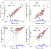 |
Fig. 1. Stellar mass, SFR, age, and dust mass (from top left to bottom right) plotted for galaxies assuming THIMF against Chabrier IMF. The estimates are derived from the SED fitting code CIGALE with errors calculated using a Bayesian analysis. The histograms on each axis show the distribution of the galaxies. Offsets in M*, SFR, and MDust among both IMFs are shown as ratios of the median values (and corresponding uncertainties from the 25th and 75th percentile of the distributions). The black dotted line in each panel represents the 1:1 relation. |
From Fig. 1, we observed that the stellar mass estimates are, on average, a factor  lower when assuming a THIMF than a Chabrier IMF. Similarly, the THIMF estimates for SFR are lower by a factor of
  than SFR derived assuming Chabrier IMF. This behavior is comparable with previous results from the literature (e.g., Wang et al. 2024). In the case of the Chabrier IMF, the predicted ages of the main stellar population of our galaxies lie on the younger end of the distribution (with mean value ∼350 Myr), whereas for the top-heavy case, the predicted ages lie on the older end (with mean value ∼650 Myr). In particular, we note that the younger galaxies in our sample tend to deviate more from the 1:1 relation, as further discussed in Sect. 4.3. Finally, we did not observe any significant difference in the dust mass between the two assumed IMFs.
For a better comparison between observations and predictions, we divided our sample into three arbitrary age bins: old (≳600 Myr), intermediate (300−600 Myr) and young galaxies (≲300 Myr). These are shown in Fig. 2, together with the relation between age and sSFR in our sources for the Chabrier and THIMF. In both cases, we obtained an almost linear relation between age and sSFR (also see, e.g., Nanni et al. 2020; Galliano et al. 2021; Burgarella et al. 2022), strengthening our comparison between evolutionary tracks and observations throughout the paper.
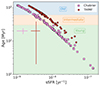 |
Fig. 2. Age of the ALPINE galaxies as a function of sSFR assuming a Chabrier IMF (pink squares) and a THIMF (red circles). The cyan, orange, and green regions represent old (≳600 Myr), intermediate (300 − 600 Myr), and young (≲300 Myr) population of galaxies. The crossbars indicate the average error on the age and sSFR for the respective sample. |
It should be noted that the estimates of the physical parameters are subject to the choice of the SFH (Leja et al. 2019; Lower et al. 2020; Whitler et al. 2023) and the attenuation law (Buat et al. 2019; Hamed et al. 2023). For instance, Topping et al. (2022) analyzed a sample of 40 UV-bright galaxies at z ∼ 7 − 8 as part of the Reionization Era Bright Emission Line Survey (REBELS; Bouwens et al. 2022). They found that the inferred stellar masses and sSFR for main-sequence galaxies in the epoch of reionization can be largely underestimated (up to an order of magnitude) if assuming a constant SFH instead of a nonparametric one. This effect is most prominent in the youngest galaxies with large sSFR and age less than 10 Myr, for which the emission from older stellar populations can be outshined by the presence of more recent bursts.
4.2. Constraining the gas content
In this section, we used our models to reproduce the gas content of our galaxies which is dictated by various physical quantities, primarily the initial gas mass (MGas, ini), the mass-loading factor (ηout) and the inflow parameter (ηin). Observational properties from the literature (i.e., gas mass, metallicity and outflow efficiency) for the ALPINE galaxies assist us to constrain the priors for our models described in Sect. 3.2.
We began by reproducing the observed gas content in the ISM of our galaxies: 68 ALPINE galaxies detected in [CII] and 30 [CII] nondetections (see Sect. 2). Specifically, we assigned an initial mass of gas to our galaxies that is proportional to their final stellar mass (normalized to 1 M⊙; see Table 2). This is a crucial parameter as it drives the evolution of galaxies over cosmic time, and it is deeply linked with their metallicity history as well as with the outflow and inflow of gas.
As mentioned in Sect. 3.2, we tested values of ηout between 0 and 3, based on observations by Ginolfi et al. (2020b). Regarding the gas-phase metallicity, given the stellar mass of our z ∼ 5 galaxies, we expect them to be characterized by a sub-solar metallicity (e.g., Faisst et al. 2016). Similar conclusions were reached by Vanderhoof et al. (2022), who measured metallicity from absorption lines in the rest-frame UV stacked spectrum of 10 ALPINE galaxies. They found an average metallicity of 12 + log(O/H) =  , corresponding to ∼50% of solar metallicity. We adopted the value 12 + log(O/H) ∼ 9.0 to constrain the terminal metallicity of the models but it should be noted that the observational value represents a small sub-sample of the ALPINE galaxies. We also varied the inflow parameter ηin in the calculations between 0 and 10.
We derived the best value of initial gas mass, inflow parameter, and SNe destruction efficiency from the best-fitting methods described in Sect. 3.5 and reported in Table 3. We then examined the variation of the outflow efficiency (ηout) on the corresponding evolutionary tracks. Fig. 3 presents the result of this analysis. We present the observed specific mass of gas (i.e., sMGas ≡ MGas/M*) as a function of specific star formation rate (i.e., sSFR ≡ SFR/M*), assuming both a Chabrier (left) and a THIMF (right), and compare these with our best predictions from models. The uncertainties in sMGas are calculated by propagating the errors from MGas (from Eq. 18) and M* (from the SED fitting). Each curve illustrates the variation of gas-phase metallicity with age, and the effect of different outflow efficiency on the history of sMGas. We ran the models for different final ages spanning the age of stellar population of the galaxies.
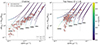 |
Fig. 3. sMGas plotted against sSFR for the ALPINE galaxies assuming a Chabrier (left) and THIMF (right). The circles represent galaxies detected via [CII], while the upper limits on gas mass are shown as inverse triangles. Evolutionary models (solid and dotted lines) are plotted for different final ages (increasing from right to left). The figure shows the case with [MGas, ini, ηout, ηin, ϵSN] ∼ [3.3, 0−2, 0.6, 0.1] and [4.4, 0−2, 0.6, 0.1] for Chabrier and THIMF, respectively. All models are color-coded by the predicted metallicity and illustrate the effect of varying ηout from 0 (solid curves) to 2 (dotted curves). |
Assuming a Chabrier IMF, we reproduced the sMGas evolution in all galaxies by adopting the optimal best-fit values MGas, ini = 3.3, ηin = 0.6, ϵSN = 0.1 from Table 3, and allowing the mass-loading factor to reach ηout = 2. A value of ηin = 0.6 is necessary to reproduce the galaxies with lower observed specific gas mass within the adopted constraints of having metallicity 12 + log(O/H) < 9.0. We anticipate solar to sub-solar metallicities for all of our sources, except for the oldest galaxies (corresponding to the lowest sSFR) for which an almost super-solar metallicity is required (12 + log(O/H) ∼ 9.0). From Fig. 3, it is clear that star formation alone (solid lines of each set of models) is not enough to deplete the gas content in the ISM of galaxies with age ≳ 300 Myr (i.e., sSFR ≲ 10−8 yr−1) galaxies. Instead, outflows play a significant role, with larger ηout needed to remove the gas more rapidly than in the ηout = 0 case. In the case of the Chabrier IMF, we require ηout ∼ 2 to successfully reproduce the observed amount of gas in older galaxies, albeit metallicity increases rapidly toward lower sSFR. Assuming a THIMF, we were able to reproduce the sMGas evolution in all galaxies but those with lowest values of sMGas by adopting MGas, ini = 4.4, ηin = 0.6, and letting the outflow efficiency to reach ηout = 2.
Although a larger mass-loading factor could be adopted in this case (i.e., ηout > 2, especially for the older sources), it would quickly exceed the observed metallicity constraints (Vanderhoof et al. 2022), as well as the observed upper limits on the outflow efficiency (Ginolfi et al. 2020b). Hence, we limit our models to ηout = 2.
4.3. Reproducing the specific dust mass
The specific dust mass (sMDust = MDust/M*) (as identified by, e.g., Rémy-Ruyer et al. 2015; Calura et al. 2017; Nanni et al. 2020) serves as a valuable metric for quantifying the dust content in galaxies as it traces the rate of dust production and/or destruction in their ISM, and can be used to disentangle the main-sequence and starburst populations (Donevski et al. 2020; Kokorev et al. 2021). The evolution of sMDust with the sSFR (or age) is also known as dust formation rate diagram (DFRD; e.g., Burgarella et al. 2022). Analyzing the DFRD provides insights into various phases of the dust cycle, including formation, destruction and transport (da Cunha et al. 2015; Michałowski et al. 2019; Nanni et al. 2020; Whitaker et al. 2021; Burgarella et al. 2022; Shivaei et al. 2022; Donevski et al. 2023; Lorenzon et al. 2025).
To model dust evolution, we based our calculations on the models described in Sect. 3.2 and we used as input parameters MGas, ini and ηin, as derived in Sect. 3.5. We determined the dust mass from the best-fitted SED using CIGALE, as described in Sects. 3.1 and 3.3. The SFR and stellar mass are also computed from the SED fitting following the same procedure as in Burgarella et al. (2022). To model the MDust, we adopted the state of the art theoretical metal yields mentioned in Table 2. The selected yields for type II SNe (SNII) are from Limongi & Chieffi (2018) and have been shown to be among those providing the highest amount of dust at the beginning of the baryon cycle (Nanni et al. 2020). The final metal yields adopted in the models are weighted for the star rotational velocities as in Prantzos et al. (2018).
In Fig. 4, we plot the DFRD for the ALPINE galaxies assuming Chabrier IMF (left) and THIMF (right). With variations in stellar mass and SFR as described in Sect. 4.1, compared to the case of Chabrier IMF (mean value for sSFRChabrier ∼ 1.5 × 10⁻⁸ yr−1), the values of sSFRTHIMF are lower (mean value ∼7.43 × 10⁻⁹ yr−1). Hence, the trend between the sMDust and sSFR shifts while assuming a THIMF with respect to Chabrier IMF owing to these deviations, and we observed lower sSFR values in the top-heavy case.
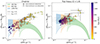 |
Fig. 4. sMDust plotted against sSFR for the ALPINE galaxies assuming a Chabrier IMF (left panel) and THIMF (right panel). The circles indicate galaxies with detected dust continuum, while inverse triangles represent upper limits on the dust mass. Dust evolution tracks are plotted for the constrained parameters [MGas, ini, ηout, ηin, ϵSN] ∼ [3.3, 0−2, 0.6, 0.1] and [4.4, 0−2, 0.6, 0.1] for the Chabrier and THIMF models, respectively, and for galaxy ages of 400 Myr, 800 Myr, and 1200 Myr for illustrative purpose. The solid color lines represent models assuming ηout = 0, while the dotted lines show the effect of increasing the outflow efficiency to ηout = 2. The models range from 25% dust condensation without dust growth in the ISM to 100% condensation with maximum dust growth efficiency. The galaxies are color-coded according to the age of their main stellar population. |
The extent of the models (i.e., from 25% of dust condensation with no dust growth in the ISM to 100% of dust condensation with maximum dust growth efficiency) is represented by the shaded region between the lower and upper bound curves for three predicted ages of the galaxies (i.e., 400, 800, 1200 Myr as representative cases) in Fig. 4. The dotted curves show the effect of adopting ηout = 2, as compared to the case with no outflow (solid patch). For the sake of clarity, we show in Fig. 4 (and in the following, in Fig. 5), only models with condensation fraction larger than 25%.
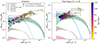 |
Fig. 5. sMDust plotted against sSFR for the ALPINE galaxies assuming a Chabrier IMF (left) and THIMF (right). The circles represent galaxies with detected continuum emission, while the inverse triangles mark the upper limits on dust mass. The contributions from the various dust sources are distinguished by the different identifiers. The mass-loading factor ranges from 0 to 2. The overall dust evolution track, which includes all contributions, is shown for the constrained parameters [MGas, ini, ηout, ηin, ϵSN] ∼ [3.3, 0−2, 0.6, 0.1] and [4.4, 0−2, 0.6, 0.1] for the Chabrier and THIMF cases, respectively, at an age ∼ 1200 Myr (hatched region). The green, pink, and brown patches represent contributions from SNII, SNIa, and AGB stars, respectively. For SNII and SNIa, the models range from 25% dust condensation with ηout = 0, to 100% condensation with ηout = 2. For AGB stars, the models vary with ηout from 0 to 2. The blue patch shows the contribution of ISM growth to the total dust content, assuming a growth efficiency of 1, varying with ηout from 0 to 2. The galaxies are color-coded based on the age of their main stellar population. |
In Fig. 5, we show the contribution of each source of dust (i.e., SNIa and SNII, AGB stars, dust growth in ISM) for Chabrier IMF (left) and THIMF (right). Contribution by the dust growth in the ISM is modeled as described by Eq. (10).
For models assuming no outflows, with Chabrier IMF, oldest galaxies with lowest values of sSFR are reproduced with condensation fractions ∼25%−30% while, assuming a THIMF, higher condensation fractions ∼50% are required to reproduce oldest galaxies. For models assuming outflows, with Chabrier IMF, a relatively moderate dust condensation fraction of ∼60% is required. The fraction rises to 75 − 85% in the case of THIMF for galaxies with the same age.
For both Chabrier and THIMF, dust growth plays a significant role for galaxies of intermediate ages (i.e., 300−600 Myr), increasing the amount of dust in their ISM of ∼60% with respect to the case with no dust growth for condensation fractions ∼50%. In the case of a condensation fraction of 5% for SNe (not shown in Fig. 5), dust growth in the ISM becomes the dominant dust production process at sSFR ≈ 2 × 10⁻⁸ yr−1 and sSFR ≈ 3 × 10⁻⁸ yr−1 for Chabrier and THIMF, respectively. For the largest condensation fraction of SNe, dust accretion in the ISM starts to dominate at sSFR ≈ 5 × 10⁻⁹ yr−1. The efficiency of dust accretion with the input parameters selected is too low in order to explain the younger galaxies.
We note that dust growth is required to reproduce the specific dust mass in galaxies of intermediate ages (i.e., 300−600 Myr), while at older ages models overpredicts the amount of dust formed even for models computed by assuming condensation fraction of 5%. Since dust in the ISM is more efficient for higher metallicity values (older ages), we may therefore expect another destruction mechanism different from outflow removal and dust destruction from astration, SNe shocks and photo-evaporation (Nanni et al. 2024), to be at work in destroying the dust grains in the ISM at older ages (≳800 Myr). This destruction mechanism can be partially due, for example, to rotational disruption of grains in strong radiation fields (Hoang et al. 2019). We also notice that within the uncertainties of the dust mass estimation (a factor of ∼3 lower than Draine et al. 2014), the galaxies of intermediate ages may be compatible with efficient dust production from SNII, without the need of dust growth in the ISM.
Furthermore, Fig. 6 shows the observed dust-to-gas (DTG) ratio as a function of the sSFR, along with our predictions from models. We calculated the DTG ratio for 68 out of 98 sources which have robust gas measurements as described in Sect. 3.4. DTG ratio also provides a solid representation of the baryonic content of the galaxies as in our study, gas and dust measurements are derived independently. As shown in Fig. 6, the DTG ratio ranges between 5 × 10⁻⁴ and 3 × 10⁻³ in the case of a Chabrier IMF, while the points result to be more scattered when assuming a THIMF. Recent observational (Donevski et al. 2020) and theoretical works employing cosmological simulations (Jones et al. 2024; Palla et al. 2024) find around similar DTG ratios.
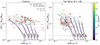 |
Fig. 6. Dust-to-gas ratio plotted against sSFR for the ALPINE galaxies assuming a Chabrier IMF (left) and a THIMF (right). Only galaxies with [CII] detections are shown. The circles represent galaxies with detected dust continuum, while the upper limits on the dust mass are indicated by inverse triangles. The evolutionary models are plotted assuming [MGas, ini, ηout, ηin, ϵSN] ∼ [3.3, 0−2, 0.6, 0.1] and [4.4, 0−2, 0.6, 0.1] for Chabrier and THIMF, respectively. The models are color-coded by predicted metallicity and illustrate the impact of varying the ηout from 0 (solid curves) to 2 (dotted curves). |
We were able to reproduce the DTG ratio for the majority of the older galaxies reaching up to 5 × 10⁻³ in the case of the Chabrier IMF, in agreement with the constraints for sMGas and sMDust (Figs. 3 and 4, left panels). Assuming a THIMF, we reproduced DTG ratios for younger galaxies and for older galaxies we reach relatively higher DTG ratios (i.e., up to 7 × 10⁻³).
5. Discussion
In the following, we discuss the contributions of the diverse mechanisms regulating the gas and dust cycle in the ISM of our galaxies. We also argue on the current limitations of the data and the models in reproducing the observables of youngest and dustier galaxies, as well as on possible solutions.
5.1. Contributions of different processes to the dust cycle
Numerous studies have investigated the nature and amount of dust in the ISM of galaxies both in the local and high-redshift Universe, suggesting different mechanisms for its production and destruction. AGB stars are considered to be the significant producers of dust in galaxies (Clemens et al. 2010; Valiante et al. 2011). However, they are not efficient on short timescales, as those typical of the early Universe (e.g., Gall et al. 2011; Dell’Agli et al. 2019; Tosi et al. 2023). Furthermore, dust can survive the SNe reverse shock (Micelotta et al. 2016; Marassi et al. 2019; Slavin et al. 2020), or directly grow in the ISM of galaxies by embedding metals from the gas phase (Asano et al. 2013; Hirashita 2015; Ginolfi et al. 2018; Aoyama et al. 2019; Donevski et al. 2020; Palla et al. 2024). Various dust destruction scenarios by SNe remnants as a result of uncertainties in the destruction efficiency are suggested where there is inefficient dust destruction in high-temperature gas (Vogelsberger et al. 2019) and enhanced dust destruction by SNe (Micelotta et al. 2018; Hu 2019; Kirchschlager et al. 2022).
In Fig. 5, we observe that, while assuming Chabrier IMF, SNII is the primary source of dust for the older galaxies (i.e., ≳600 Myr). The AGB contribution becomes prominent toward the later stages of their evolution (age ≳ 1000 Myr), and can dominate their total dust production provided that the condensation fraction is less than 25% for SNII for the case that no dust growth in ISM is present. The contribution from SNIa is always negligible as compared to SNII and AGB together (∼0.001% of total dust content). Assuming no dust growth, we can reproduce ∼30% of galaxies (with age ≳ 300 Myr) when ηout = 0 (i.e., assuming no galactic outflow), owing to contribution from SNII and AGB. Considering the case of models with outflows, we can reproduce similar percentage of the sample but assuming higher condensation fractions (∼50%) for SNII. The latter scenario is likely more reliable given the ubiquitous observations of star formation driven outflows in both local and high-z sources (Romano et al. 2023, 2024; Mitsuhashi et al. 2024), and specifically because of the evidence for feedback found in ALPINE (Ginolfi et al. 2020b). Furthermore, dust growth in the ISM takes over as the major contributor to the dust content where SNII are insufficient with extreme condensation fractions for galaxies with intermediate ages (i.e., 300−600 Myr). Similar conclusions have been presented for REBELS survey (z ∼ 7, Algera et al. 2024), where dust growth in ISM is necessary to reproduce dust masses in high-z galaxies.
Figure 4 shows the gradual trend in the dust cycles as we vary the mass-loading factor. Higher ηout leads to more outflow of gas which is reflected in the trends for models plotted for sMgas in Fig. 3 and for sMDust in Fig. 4. With increasing ηout, the contributions from SNII are offset by the dust growth in ISM which takes over to be the primary contributor to the dust content of the older galaxies (age ≳ 800 Myr). The dust content in the younger galaxies is denoted by high values of specific dust mass for high values of specific star formation rate. The rapid dust buildup observed in galaxies younger than 500 Myr is not reproducible when considering traditional IMF (i.e., Chabrier IMF). Hence, a different form of IMF is tested and explained in the next section.
5.2. Effect of different IMFs
As discussed in Sect. 3, we assumed a THIMF introducing a population of short-lived massive stars. The effect of this assumption is reflected in the results represented in Fig. 5 (right) where SNII are the primary source of dust for the galaxies with age ≳ 300 Myr. Due to the short lives and rapid stellar evolution, the dust buildup observed in the younger galaxies is reproduced with the models reaching larger sMDust values in timescales of 400 Myr−500 Myr. In the case of models with no dust growth in ISM (right panel of Fig. 5), galaxies with age ∼800 Myr are reproduced owing to the contributions from SNII and AGB stars assuming no outflow (ηout = 0) and condensation fractions for SNII limited to moderate values (∼25%). For the galaxies that reach higher values of sMDust in shorter timescales (∼300 Myr), dust growth in ISM is required to reproduce the observations, hence being the primary contributor to the dust content of the galaxies as contributions from SNII and AGB prove to be insufficient. At the same time, if dust growth is considered, we overproduce dust for older galaxies. In the case of ηout = 2, dust contribution from SNII reproduced galaxies with higher values of sMDust even at older ages only if condensation fraction is ≳80% assuming no dust growth.
In Fig. 6 (right), we probe the DTG ratio for the galaxies assuming a THIMF, where the models reproduce the DTG ratio for the younger galaxies which are observed to have higher sMDust (Fig. 5, right panel), given that MGas, ini is greater than that in the case of Chabrier. Assuming a THIMF helps in reproducing higher sMDust values but not higher DTG ratios as THIMF favors rapid dust production from SNII and faster dust growth but at the same time also enhances gas content in the ISM due to the larger mass ejection rates from evolved stellar populations (Palla et al. 2020).
Generally, in the case of THIMF, it is observed that AGB stars are not contributing significantly in contrast to their contribution when considering the Chabrier IMF. These cumulative trends hint that the nature of dust production and destruction is variational and different in various stages of galactic evolution. In Fig. 5 (right), we observe that the THIMF falls short for younger galaxies (≲100 Myr) with higher values of sMDust (≳10−2). This can be attributed to limited understanding of the mechanisms at play in high-z universe or overestimation of derived parameters from SED fitting of the galaxies, thus hinting at the need of emendation of our models.
For such galaxies, we examined variations in the SED fitting and evolution models in relation to the rest of the sample, with the goal of reproducing their dust content in Figs. 4 and 5. Our initial tests focused on the possibility that these galaxies possess a larger gas mass, which could explain the values of sMGas shown in Fig. 3. These values could only be satisfied under the assumption of a THIMF. In contrast, for a Chabrier IMF, increasing the gas mass – whether by adjusting the initial gas mass (MGas, ini) or increasing the inflow rate via ηin, failed to reproduce the properties of the youngest galaxies (sMGas) shown in the left panel of Fig. 3, as increased gas content in the models would, in theory, reduce the efficiency of dust destruction by SNe and dust removal through outflows (see Eqs. 6, 8, and 9). However, even under the assumption of maximal condensation fractions of metal into dust grains, the predicted sMDust does not reach the observed values.
We further explored the possibility of different star formation history, using a delayed plus burst model (Boquien et al. 2019). In this scenario, we re-fitted the sources by allowing the fraction of stars to form in the burst, the age of the stellar population, the burst e-folding time, and the burst age to vary as free parameters. Despite these variations, the sMDust derived for the youngest galaxies remains too large to be reproduced by the current models.
5.3. Comparison with different dust models
As shown in Figs. 4, 5 and discussed in Sect. 5.2, the implementation of a THIMF can alleviate the tension between the observed and predicted amount of dust in the ISM of high-z galaxies. In spite of this, a few sources with high sMDust and sSFR still exceed the theoretical expectations, challenging our comprehension of galaxy formation at early times.
Previous attempts of reproducing the observed dust masses in z > 4 galaxies have faced similar difficulties. Dayal et al. (2022) made use of the DELPHI semi-analytical model to explain the dust content in the ISM of 13 galaxies detected in [CII] and dust continuum as part of the REBELS program, whose targets were selected in a comparable way as for ALPINE but at higher redshift (z > 6) and show similar properties in terms of gas mass, sSFR, and sMDust (e.g., Dayal et al. 2022; Palla et al. 2024). Their fiducial model (which includes the combined effect of SNII, astration, destruction and removal of dust by shocks and outflows, and a grain growth timescale of ∼30 Myr) was able to reproduce the majority of those galaxies, anticipating a typical sMDust ∼ 10−3, that is comparable with our predictions (see Figs. 4, 5). On the other hand, the same model struggled to reproduce the youngest, low-mass galaxies in their sample (i.e., sources with the largest sSFR), for which extreme assumptions on dust production (i.e., a rapid grain growth with a timescale below 1 Myr, no dust destruction by SNe shocks or no ejection by outflows) were needed instead, leading to ∼1 dex larger sMDust.
Di Cesare et al. (2023) investigated the dust buildup process in z > 4 galaxies by means of cosmological simulations performed with the DUSTYGADGET code (Graziani et al. 2020). By taking into account dust production by SNe, AGB stars, and grain growth in the ISM, as well as destruction/removal by shocks, astration, and sputtering, their simulations reproduce large amounts of dust (sMDust ∼ 10−2) in galaxies with log10(M*/M⊙) ≳ 10. This implies a slight overproduction of dust as compared to our models assuming a Chabrier IMF that can be due, for example, to a shorter timescale of dust accretion in the ISM (Graziani et al. 2020; Di Cesare et al. 2023). Still, those models fail in reproducing less-massive galaxies with very large sMDust (e.g., Witstok et al. 2022). Recently, Palla et al. (2024) used chemical evolution models to investigate dust evolution in the REBELS survey, exploring the impact of different metallicity enrichment of the ISM on predictions for the dominant dust production and/or destruction mechanisms. They found that both a fast or milder dust buildup evolution is needed to reproduce the dust content or DGR for their sources, with specific dust of mass reaching up to sMDust ∼ 10−2. However, they also underpredict the observed amount of dust for younger galaxies with the lowest stellar masses (log10(M*/M⊙) ∼ 9), suggesting that for these objects a THIMF may be adopted. Finally, Pozzi et al. (2021) compared the observed dust and gas masses of the continuum-detected ALPINE sources with evolutionary tracks from chemical models by Calura et al. (2008, 2014) for galaxies with different morphological types, namely spiral galaxies and proto-spheroids (the latter being progenitors of local elliptical galaxies). In spite of their large dust masses (up to ∼1 dex larger than our estimates given their assumption on low dust temperatures; see also Sect. 4.1), their proto-spheroids models were able to reproduce the majority of the galaxies, even those at the highest sMDust, reaching values up to ∼10−1.5 for tracks with final mass of log10(M*/M⊙) ∼ 10. These results seem to be in contrast with the maximum dust production found in this work, as well as in the above-mentioned models from the literature (e.g., Dayal et al. 2022; Di Cesare et al. 2023; Palla et al. 2024). However, it must be noted that the prescriptions about the dust production and/or destruction processes in Calura et al. (2008) and in the other models can present substantial differences. For instance, Calura et al. (2008) tailored their chemical evolution on galaxies with specific morphological types with varied star formation histories. Furthermore, they do not directly include the effect of outflows in the models, rather they instantaneously eject all the gas out of the galaxy when the energy deposited in the ISM by SNe equals the binding energy of the gas (Calura et al. 2008). Such a differences could explain the discrepancy with other predictions.
6. Conclusions
In this work we employed chemical evolution models to reproduce the observed gas and dust content in z ∼ 5 main-sequence star-forming galaxies as drawn from the ALMA Large Program ALPINE. We derived the physical parameters (SFR, dust mass, stellar mass) and constrained the physical processes influencing gas and dust production and/or consumption in their ISM. Specifically, we investigated the impact of the initial gas mass, outflow mass-loading factor, and inflow parameter on the models, and we tested our results on canonical (i.e., Chabrier) or top-heavy IMFs. Our main findings are summarized below:
-
Galactic outflows are essential for reproducing the decrease in the observed gas mass with increasing age, while keeping the gas-phase metallicity close to (or below) solar. Outflow efficiencies on the order of ∼2 are especially needed for galaxies ≳300 Myr old (see Fig. 3), while lower ηout values are viable for younger sources.
-
Regardless of the adopted IMF, the amount of dust in older galaxies (≳600 Myr) can be reproduced with a major contribution from SNII assuming a condensation fraction of ≳50%, and with no need for dust growth in the ISM. However, in galaxies of intermediate ages (i.e., 300 − 600 Myr), dust growth starts playing a significant role, allowing a ∼60% larger amount of dust. We note that if dust growth in the ISM increases with metallicity, as predicted by models (e.g., Asano et al. 2013), another destruction mechanism should be at work in order to reproduce the galaxies at older ages. This mechanism may be for example rotational disruption of grains exposed to strong radiation fields. Alternatively, the observed dust masses may be overestimated by a factor of ≈50% (Burgarella et al. 2022).
-
Dust production from SNIa is negligible at all ages for both IMFs. In the case of THIMF, AGB stars also do not play a major role. However, they begin to contribute ≳10% for ages ≳800 Myr if assuming a Chabrier IMF (see Fig. 5).
-
We find that 65% of our galaxies can be reproduced with a canonical Chabrier IMF. The fraction increases to 93% when adopting a THIMF. A flatter slope of the IMF could thus help in alleviating the tension between observations and models for galaxies at the first stages of the dust cycle, although it is still not enough to reproduce the youngest and dustiest sources of our sample (sSFR ≳ 10−8 yr−1, sMDust ≳ 10−2).
Our work highlights the importance of chemical evolutionary models while probing the baryon cycle of primordial galaxies. Although our results seem to suggest the need for a THIMF to allow a fast production of dust in the youngest sources, further investigation is essential. In this regard, follow-up observations with ALMA are required to sample the peak of the FIR SED of our galaxies, allowing a better constraint of the dust mass estimates. Furthermore, we are currently taking advantage of a completed JWST/NIRSpec IFU program (ID: 3045, PI: A. Faisst), which collected observations of 18 ALPINE galaxies at kiloparsec scales in the rest-frame optical regime, covering several emission lines including [OIII] and Hα. This program will allow us to put robust constraints on the stellar masses, SFHs, and metallicities of our galaxies, and to calibrate our models for a more in-depth and thorough description of galaxy formation at early times.
We refer here to sources lying on the main sequence of star-forming galaxies, i.e., with a tight relation between star formation rate (SFR) and stellar mass (e.g., Speagle et al. 2014).
In Ginolfi et al. (2020b), it is assumed that [CII] is mostly tracing the atomic gas. If also the ionized and molecular gas are contributing at the same level to the outflow, then ηout, TOT = 3 × ηout, [CII].
We define as “key element” the least abundant among the elements that form a certain dust species divided by its number of atoms in the compound (Ferrarotti & Gail 2006).
Throughout the paper, we adopt the instantaneous SFR from CIGALE (see Boquien et al. 2019 for more details), which allows us to make a better comparison with SFR predicted by models at each time-step.
Pozzi et al. (2021) also assumed higher dust temperature ∼35 K, which reduced their dust estimates by 60% with respect to their fiducial model, resulting in a better agreement with this work.
Acknowledgments
We warmly thank the referee for her/his useful comments and suggestions that greatly improved the quality of our paper. P.S., A.N., and M.R. acknowledge support from the Narodowe Centrum Nauki (UMO-2020/38/E/ST9/00077). M.R. acknowledges support from the Foundation for Polish Science (FNP) under the program START 063.2023. D.D. acknowledges support from the National Science Center (NCN) grant SONATA (UMO-2020/39/D/ST9/00720). J. and K.M. are grateful for the support from the Polish National Science Centre via grant UMO-2018/30/E/ST9/00082. J. acknowledges support from the European Union (MSCA EDUCADO, GA 101119830 and WIDERA ExGal-Twin, GA 101158446). M.B. gratefully acknowledges support from the ANID BASAL project FB210003 and from the FONDECYT regular grant 1211000. This work was supported by the French government through the France 2030 investment plan managed by the National Research Agency (ANR), as part of the Initiative of Excellence of Université Côte d’Azur under reference number ANR-15-IDEX-01. M.H. acknowledges support from the Polish National Science Center (UMO-2022/45/N/ST9/01336). E.I. acknowledges funding by ANID FONDECYT Regular 1221846. G.E.M. acknowledges the Villum Fonden research grant 13160 “Gas to stars, stars to dust: tracing star formation across cosmic time”, grant 37440, “The Hidden Cosmos”, and the Cosmic Dawn Center of Excellence funded by the Danish National Research Foundation under the grant No. 140.
References
- Algera, H. S. B., Inami, H., Oesch, P. A., et al. 2023, MNRAS, 518, 6142 [Google Scholar]
- Algera, H. S. B., Inami, H., Sommovigo, L., et al. 2024, MNRAS, 527, 6867 [Google Scholar]
- Allison, J. R., Mahony, E. K., Moss, V. A., et al. 2019, MNRAS, 482, 2934 [NASA ADS] [Google Scholar]
- Aoyama, S., Hirashita, H., Lim, C.-F., et al. 2019, MNRAS, 484, 1852 [NASA ADS] [CrossRef] [Google Scholar]
- Asano, R. S., Takeuchi, T. T., Hirashita, H., & Inoue, A. K. 2013, Earth Planets Space, 65, 213 [NASA ADS] [CrossRef] [Google Scholar]
- Asplund, M., Grevesse, N., Sauval, A. J., & Scott, P. 2009, ARA&A, 47, 481 [NASA ADS] [CrossRef] [Google Scholar]
- Bakx, T. J. L. C., Sommovigo, L., Carniani, S., et al. 2021, MNRAS, 508, L58 [NASA ADS] [CrossRef] [Google Scholar]
- Barger, A. J., Cowie, L. L., Sanders, D. B., et al. 1998, Nature, 394, 248 [Google Scholar]
- Bekki, K., & Tsujimoto, T. 2023, MNRAS, 526, L26 [NASA ADS] [CrossRef] [Google Scholar]
- Béthermin, M., Daddi, E., Magdis, G., et al. 2015, A&A, 573, A113 [Google Scholar]
- Béthermin, M., Wu, H.-Y., Lagache, G., et al. 2017, A&A, 607, A89 [Google Scholar]
- Béthermin, M., Fudamoto, Y., Ginolfi, M., et al. 2020, A&A, 643, A2 [Google Scholar]
- Boquien, M., Burgarella, D., Roehlly, Y., et al. 2019, A&A, 622, A103 [NASA ADS] [CrossRef] [EDP Sciences] [Google Scholar]
- Boquien, M., Buat, V., Burgarella, D., et al. 2022, A&A, 663, A50 [NASA ADS] [CrossRef] [EDP Sciences] [Google Scholar]
- Bouwens, R. J., Aravena, M., Decarli, R., et al. 2016, ApJ, 833, 72 [NASA ADS] [CrossRef] [Google Scholar]
- Bouwens, R. J., Smit, R., Schouws, S., et al. 2022, ApJ, 931, 160 [NASA ADS] [CrossRef] [Google Scholar]
- Boylan-Kolchin, M. 2023, Nat. Astron., 7, 731 [NASA ADS] [CrossRef] [Google Scholar]
- Brown, T., & Wilson, C. D. 2019, ApJ, 879, 17 [NASA ADS] [CrossRef] [Google Scholar]
- Bruzual, G., & Charlot, S. 2003, MNRAS, 344, 1000 [NASA ADS] [CrossRef] [Google Scholar]
- Buat, V., Ciesla, L., Boquien, M., Małek, K., & Burgarella, D. 2019, A&A, 632, A79 [NASA ADS] [CrossRef] [EDP Sciences] [Google Scholar]
- Burgarella, D., Buat, V., & Iglesias-Páramo, J. 2005, MNRAS, 360, 1413 [NASA ADS] [CrossRef] [Google Scholar]
- Burgarella, D., Bogdanoska, J., Nanni, A., et al. 2022, A&A, 664, A73 [NASA ADS] [CrossRef] [EDP Sciences] [Google Scholar]
- Calura, F., Pipino, A., & Matteucci, F. 2008, A&A, 479, 669 [NASA ADS] [CrossRef] [EDP Sciences] [Google Scholar]
- Calura, F., Gilli, R., Vignali, C., et al. 2014, MNRAS, 438, 2765 [NASA ADS] [CrossRef] [Google Scholar]
- Calura, F., Pozzi, F., Cresci, G., et al. 2017, MNRAS, 465, 54 [Google Scholar]
- Calura, F., Palla, M., Morselli, L., et al. 2023, MNRAS, 523, 2351 [NASA ADS] [CrossRef] [Google Scholar]
- Calzetti, D., Armus, L., Bohlin, R. C., et al. 2000, ApJ, 533, 682 [NASA ADS] [CrossRef] [Google Scholar]
- Capak, P. L., Carilli, C., Jones, G., et al. 2015, Nature, 522, 455 [NASA ADS] [CrossRef] [Google Scholar]
- Cappellari, M., McDermid, R. M., Alatalo, K., et al. 2012, Nature, 484, 485 [Google Scholar]
- Cardamone, C. N., van Dokkum, P. G., Urry, C. M., et al. 2010, ApJS, 189, 270 [Google Scholar]
- Carilli, C. L., Riechers, D., Walter, F., et al. 2013, ApJ, 763, 120 [NASA ADS] [CrossRef] [Google Scholar]
- Casey, C. M., Scoville, N. Z., Sanders, D. B., et al. 2014, ApJ, 796, 95 [NASA ADS] [CrossRef] [Google Scholar]
- Casey, C. M., Zavala, J. A., Spilker, J., et al. 2018, ApJ, 862, 77 [Google Scholar]
- Chabrier, G. 2003, PASP, 115, 763 [Google Scholar]
- Christensen, C. R., Davé, R., Brooks, A., Quinn, T., & Shen, S. 2018, ApJ, 867, 142 [CrossRef] [Google Scholar]
- Clemens, M. S., Jones, A. P., Bressan, A., et al. 2010, A&A, 518, L50 [NASA ADS] [CrossRef] [EDP Sciences] [Google Scholar]
- Cochrane, R. K., Hayward, C. C., Anglés-Alcázar, D., & Somerville, R. S. 2023, MNRAS, 518, 5522 [Google Scholar]
- Combes, F., Rex, M., Rawle, T. D., et al. 2012, A&A, 538, L4 [NASA ADS] [CrossRef] [EDP Sciences] [Google Scholar]
- Côté, B., O’Shea, B. W., Ritter, C., Herwig, F., & Venn, K. A. 2017, ApJ, 835, 128 [Google Scholar]
- Cousin, M., Buat, V., Lagache, G., & Bethermin, M. 2019, A&A, 627, A132 [NASA ADS] [CrossRef] [EDP Sciences] [Google Scholar]
- Cristallo, S., Straniero, O., Piersanti, L., & Gobrecht, D. 2015, ApJS, 219, 40 [Google Scholar]
- da Cunha, E., Walter, F., Smail, I. R., et al. 2015, ApJ, 806, 110 [Google Scholar]
- Dabringhausen, J., Kroupa, P., Pflamm-Altenburg, J., & Mieske, S. 2012, ApJ, 747, 72 [NASA ADS] [CrossRef] [Google Scholar]
- Davé, R., Anglés-Alcázar, D., Narayanan, D., et al. 2019, MNRAS, 486, 2827 [Google Scholar]
- Dayal, P., Ferrara, A., Sommovigo, L., et al. 2022, MNRAS, 512, 989 [NASA ADS] [CrossRef] [Google Scholar]
- De Looze, I., Cormier, D., Lebouteiller, V., et al. 2014, A&A, 568, A62 [NASA ADS] [CrossRef] [EDP Sciences] [Google Scholar]
- De Looze, I., Lamperti, I., Saintonge, A., et al. 2020, MNRAS, 496, 3668 [NASA ADS] [CrossRef] [Google Scholar]
- Dell’Agli, F., Valiante, R., Kamath, D., Ventura, P., & García-Hernández, D. A. 2019, MNRAS, 486, 4738 [Google Scholar]
- Dessauges-Zavadsky, M., Ginolfi, M., Pozzi, F., et al. 2020, A&A, 643, A5 [NASA ADS] [CrossRef] [EDP Sciences] [Google Scholar]
- Di Cesare, C., Graziani, L., Schneider, R., et al. 2023, MNRAS, 519, 4632 [Google Scholar]
- Donevski, D., Buat, V., Boone, F., et al. 2018, A&A, 614, A33 [NASA ADS] [CrossRef] [EDP Sciences] [Google Scholar]
- Donevski, D., Lapi, A., Małek, K., et al. 2020, A&A, 644, A144 [NASA ADS] [CrossRef] [EDP Sciences] [Google Scholar]
- Donevski, D., Damjanov, I., Nanni, A., et al. 2023, A&A, 678, A35 [NASA ADS] [CrossRef] [EDP Sciences] [Google Scholar]
- Draine, B. T., & Li, A. 2007, ApJ, 657, 810 [CrossRef] [Google Scholar]
- Draine, B. T., Aniano, G., Krause, O., et al. 2014, ApJ, 780, 172 [Google Scholar]
- Dudzevičiūtė, U., Smail, I., Swinbank, A. M., et al. 2020, MNRAS, 494, 3828 [Google Scholar]
- Dunlop, J. S., McLure, R. J., Biggs, A. D., et al. 2017, MNRAS, 466, 861 [Google Scholar]
- Faisst, A. L., Capak, P. L., Davidzon, I., et al. 2016, ApJ, 822, 29 [Google Scholar]
- Faisst, A. L., Schaerer, D., Lemaux, B. C., et al. 2020, ApJS, 247, 61 [NASA ADS] [CrossRef] [Google Scholar]
- Ferrarotti, A. S., & Gail, H. P. 2006, A&A, 447, 553 [CrossRef] [EDP Sciences] [Google Scholar]
- Fudamoto, Y., Ivison, R. J., Oteo, I., et al. 2017, MNRAS, 472, 2028 [NASA ADS] [CrossRef] [Google Scholar]
- Fudamoto, Y., Oesch, P. A., Magnelli, B., et al. 2020, MNRAS, 491, 4724 [Google Scholar]
- Fujimoto, S., Silverman, J. D., Bethermin, M., et al. 2020, ApJ, 900, 1 [Google Scholar]
- Gall, C., & Hjorth, J. 2018, ApJ, 868, 62 [CrossRef] [Google Scholar]
- Gall, C., Andersen, A. C., & Hjorth, J. 2011, A&A, 528, A13 [NASA ADS] [CrossRef] [EDP Sciences] [Google Scholar]
- Galliano, F., Nersesian, A., Bianchi, S., et al. 2021, A&A, 649, A18 [EDP Sciences] [Google Scholar]
- Geha, M., Brown, T. M., Tumlinson, J., et al. 2013, ApJ, 771, 29 [NASA ADS] [CrossRef] [Google Scholar]
- Giavalisco, M., Ferguson, H. C., Koekemoer, A. M., et al. 2004, ApJ, 600, L93 [NASA ADS] [CrossRef] [Google Scholar]
- Ginolfi, M., Graziani, L., Schneider, R., et al. 2018, MNRAS, 473, 4538 [NASA ADS] [CrossRef] [Google Scholar]
- Ginolfi, M., Jones, G. C., Béthermin, M., et al. 2020a, A&A, 643, A7 [NASA ADS] [CrossRef] [EDP Sciences] [Google Scholar]
- Ginolfi, M., Jones, G. C., Béthermin, M., et al. 2020b, A&A, 633, A90 [NASA ADS] [CrossRef] [EDP Sciences] [Google Scholar]
- González-López, J., Novak, M., Decarli, R., et al. 2020, ApJ, 897, 91 [Google Scholar]
- Graziani, L., Schneider, R., Ginolfi, M., et al. 2020, MNRAS, 494, 1071 [NASA ADS] [CrossRef] [Google Scholar]
- Gruppioni, C., Béthermin, M., Loiacono, F., et al. 2020, A&A, 643, A8 [NASA ADS] [CrossRef] [EDP Sciences] [Google Scholar]
- Guo, Y., Ferguson, H. C., Giavalisco, M., et al. 2013, ApJS, 207, 24 [NASA ADS] [CrossRef] [Google Scholar]
- Hamed, M., Małek, K., Buat, V., et al. 2023, ArXiv e-prints [arXiv:2308.10672] [Google Scholar]
- Hasinger, G., Cappelluti, N., Brunner, H., et al. 2007, ApJS, 172, 29 [NASA ADS] [CrossRef] [Google Scholar]
- Hasinger, G., Capak, P., Salvato, M., et al. 2018, ApJ, 858, 77 [Google Scholar]
- Heger, A., & Woosley, S. E. 2010, ApJ, 724, 341 [Google Scholar]
- Heinis, S., Buat, V., Béthermin, M., et al. 2014, MNRAS, 437, 1268 [Google Scholar]
- Hezaveh, Y. D., Marrone, D. P., Fassnacht, C. D., et al. 2013, ApJ, 767, 132 [NASA ADS] [CrossRef] [Google Scholar]
- Hirashita, H. 2015, MNRAS, 447, 2937 [NASA ADS] [CrossRef] [Google Scholar]
- Hoang, T., Tram, L. N., Lee, H., & Ahn, S.-H. 2019, Nat. Astron., 3, 766 [Google Scholar]
- Hodge, J. A., & da Cunha, E. 2020, Roy. Soc. Open Sci., 7, 200556 [NASA ADS] [CrossRef] [Google Scholar]
- Hodge, J. A., Karim, A., Smail, I., et al. 2013, ApJ, 768, 91 [Google Scholar]
- Hou, K.-C., Aoyama, S., Hirashita, H., Nagamine, K., & Shimizu, I. 2019, MNRAS, 485, 1727 [NASA ADS] [CrossRef] [Google Scholar]
- Hu, C.-Y. 2019, MNRAS, 483, 3363 [NASA ADS] [CrossRef] [Google Scholar]
- Hughes, D. H., Serjeant, S., Dunlop, J., et al. 1998, Nature, 394, 241 [Google Scholar]
- Inami, H., Algera, H. S. B., Schouws, S., et al. 2022, MNRAS, 515, 3126 [NASA ADS] [CrossRef] [Google Scholar]
- Inayoshi, K., Harikane, Y., Inoue, A. K., Li, W., & Ho, L. C. 2022, ApJ, 938, L10 [NASA ADS] [CrossRef] [Google Scholar]
- Ivison, R. J., Swinbank, A. M., Swinyard, B., et al. 2010, A&A, 518, L35 [NASA ADS] [CrossRef] [EDP Sciences] [Google Scholar]
- Iwamoto, K., Brachwitz, F., Nomoto, K., et al. 1999, ApJS, 125, 439 [NASA ADS] [CrossRef] [Google Scholar]
- Jin, S., Daddi, E., Magdis, G. E., et al. 2019, ApJ, 887, 144 [Google Scholar]
- Johnson, N., Kotz, S., & Balakrishnan, N. 1995, Continuous Univariate Distributions, Volume 2, Wiley Series in Probability and Statistics (Wiley) [Google Scholar]
- Jones, G. C., Vergani, D., Romano, M., et al. 2021, MNRAS, 507, 3540 [NASA ADS] [CrossRef] [Google Scholar]
- Jones, E., Smith, B., Davé, R., Narayanan, D., & Li, Q. 2024, MNRAS, 535, 1293 [NASA ADS] [CrossRef] [Google Scholar]
- Kirchschlager, F., Mattsson, L., & Gent, F. A. 2022, MNRAS, 509, 3218 [Google Scholar]
- Koekemoer, A. M., Aussel, H., Calzetti, D., et al. 2007, ApJS, 172, 196 [Google Scholar]
- Kokorev, V. I., Magdis, G. E., Davidzon, I., et al. 2021, ApJ, 921, 40 [NASA ADS] [CrossRef] [Google Scholar]
- Koprowski, M. P., Coppin, K. E. K., Geach, J. E., et al. 2020, MNRAS, 492, 4927 [NASA ADS] [CrossRef] [Google Scholar]
- Kroupa, P., Weidner, C., Pflamm-Altenburg, J., et al. 2013, in Planets, Stars and Stellar Systems. Volume 5: Galactic Structure and Stellar Populations, eds. T. D. Oswalt, & G. Gilmore, 5, 115 [NASA ADS] [Google Scholar]
- Labbé, I., van Dokkum, P., Nelson, E., et al. 2023, Nature, 616, 266 [CrossRef] [Google Scholar]
- Lacey, C. G., Baugh, C. M., Frenk, C. S., et al. 2016, MNRAS, 462, 3854 [Google Scholar]
- Lagache, G., Cousin, M., & Chatzikos, M. 2018, A&A, 609, A130 [NASA ADS] [CrossRef] [EDP Sciences] [Google Scholar]
- Lagos, C. D. P., Robotham, A. S. G., Trayford, J. W., et al. 2019, MNRAS, 489, 4196 [NASA ADS] [CrossRef] [Google Scholar]
- Laporte, N., Ellis, R. S., Boone, F., et al. 2017, ApJ, 837, L21 [CrossRef] [Google Scholar]
- Larson, R. B. 1998, MNRAS, 301, 569 [NASA ADS] [CrossRef] [Google Scholar]
- Le Fèvre, O., Tasca, L. A. M., Cassata, P., et al. 2015, A&A, 576, A79 [Google Scholar]
- Le Fèvre, O., Béthermin, M., Faisst, A., et al. 2020, A&A, 643, A1 [Google Scholar]
- Leja, J., Carnall, A. C., Johnson, B. D., Conroy, C., & Speagle, J. S. 2019, ApJ, 876, 3 [Google Scholar]
- Lemaux, B. C., Le Floc’h, E., Le Fèvre, O., et al. 2014, A&A, 572, A90 [NASA ADS] [CrossRef] [EDP Sciences] [Google Scholar]
- Limongi, M., & Chieffi, A. 2018, ApJS, 237, 13 [NASA ADS] [CrossRef] [Google Scholar]
- Liu, D., Schinnerer, E., Groves, B., et al. 2019, ApJ, 887, 235 [Google Scholar]
- Lorenzon, G., Donevski, D., Lisiecki, K., et al. 2025, A&A, 693, A118 [NASA ADS] [CrossRef] [EDP Sciences] [Google Scholar]
- Lovell, C. C., Geach, J. E., Davé, R., Narayanan, D., & Li, Q. 2021, MNRAS, 502, 772 [NASA ADS] [CrossRef] [Google Scholar]
- Lower, S., Narayanan, D., Leja, J., et al. 2020, ApJ, 904, 33 [NASA ADS] [CrossRef] [Google Scholar]
- Magnelli, B., Popesso, P., Berta, S., et al. 2013, A&A, 553, A132 [NASA ADS] [CrossRef] [EDP Sciences] [Google Scholar]
- Marassi, S., Schneider, R., Limongi, M., et al. 2019, MNRAS, 484, 2587 [NASA ADS] [CrossRef] [Google Scholar]
- Marks, M., Kroupa, P., Dabringhausen, J., & Pawlowski, M. S. 2012, MNRAS, 422, 2246 [NASA ADS] [CrossRef] [Google Scholar]
- Martín-Navarro, I., La Barbera, F., Vazdekis, A., Falcón-Barroso, J., & Ferreras, I. 2015, MNRAS, 447, 1033 [Google Scholar]
- Mathis, J. S., Rumpl, W., & Nordsieck, K. H. 1977, ApJ, 217, 425 [Google Scholar]
- McCracken, H. J., Milvang-Jensen, B., Dunlop, J., et al. 2012, A&A, 544, A156 [NASA ADS] [CrossRef] [EDP Sciences] [Google Scholar]
- McKinnon, R., Torrey, P., Vogelsberger, M., Hayward, C. C., & Marinacci, F. 2017, MNRAS, 468, 1505 [NASA ADS] [CrossRef] [Google Scholar]
- McMullin, J. P., Waters, B., Schiebel, D., Young, W., & Golap, K. 2007, ASP Conf. Ser., 376, 127 [Google Scholar]
- McWilliam, A., Wallerstein, G., & Mottini, M. 2013, ApJ, 778, 149 [NASA ADS] [CrossRef] [Google Scholar]
- Micelotta, E. R., Dwek, E., & Slavin, J. D. 2016, A&A, 590, A65 [NASA ADS] [CrossRef] [EDP Sciences] [Google Scholar]
- Micelotta, E. R., Matsuura, M., & Sarangi, A. 2018, Space Sci. Rev., 214, 53 [NASA ADS] [CrossRef] [Google Scholar]
- Michałowski, M. J., Hjorth, J., Gall, C., et al. 2019, A&A, 632, A43 [NASA ADS] [CrossRef] [EDP Sciences] [Google Scholar]
- Mitsuhashi, I., Tadaki, K.-I., Ikeda, R., et al. 2024, A&A, 690, A197 [NASA ADS] [CrossRef] [EDP Sciences] [Google Scholar]
- Nanni, A., Bressan, A., Marigo, P., & Girardi, L. 2013, MNRAS, 434, 2390 [NASA ADS] [CrossRef] [Google Scholar]
- Nanni, A., Burgarella, D., Theulé, P., Côté, B., & Hirashita, H. 2020, A&A, 641, A168 [NASA ADS] [CrossRef] [EDP Sciences] [Google Scholar]
- Nanni, A., Cristallo, S., Donevski, D., et al. 2024, A&A, 684, A163 [NASA ADS] [CrossRef] [EDP Sciences] [Google Scholar]
- Narayanan, D., Turk, M., Feldmann, R., et al. 2015, Nature, 525, 496 [NASA ADS] [CrossRef] [Google Scholar]
- Nayyeri, H., Cooray, A., Jullo, E., et al. 2017, ApJ, 844, 82 [NASA ADS] [CrossRef] [Google Scholar]
- Noll, S., Burgarella, D., Giovannoli, E., et al. 2009, A&A, 507, 1793 [NASA ADS] [CrossRef] [EDP Sciences] [Google Scholar]
- Palla, M., Calura, F., Matteucci, F., et al. 2020, MNRAS, 494, 2355 [NASA ADS] [CrossRef] [Google Scholar]
- Palla, M., De Looze, I., Relaño, M., et al. 2024, MNRAS, 528, 2407 [NASA ADS] [CrossRef] [Google Scholar]
- Pantoni, L., Lapi, A., Massardi, M., Goswami, S., & Danese, L. 2019, ApJ, 880, 129 [NASA ADS] [CrossRef] [Google Scholar]
- Pantoni, L., Massardi, M., Lapi, A., et al. 2021, MNRAS, 507, 3998 [CrossRef] [Google Scholar]
- Popping, G., Somerville, R. S., & Galametz, M. 2017, MNRAS, 471, 3152 [NASA ADS] [CrossRef] [Google Scholar]
- Pozzi, F., Calura, F., Fudamoto, Y., et al. 2021, A&A, 653, A84 [NASA ADS] [CrossRef] [EDP Sciences] [Google Scholar]
- Prantzos, N., Abia, C., Limongi, M., Chieffi, A., & Cristallo, S. 2018, MNRAS, 476, 3432 [Google Scholar]
- Priestley, F. D., De Looze, I., & Barlow, M. J. 2022, MNRAS, 509, L6 [Google Scholar]
- Rémy-Ruyer, A., Madden, S. C., Galliano, F., et al. 2015, A&A, 582, A121 [Google Scholar]
- Riechers, D. A., Bradford, C. M., Clements, D. L., et al. 2013, Nature, 496, 329 [Google Scholar]
- Riechers, D. A., Carilli, C. L., Capak, P. L., et al. 2014, ApJ, 796, 84 [Google Scholar]
- Robson, E. I., Ivison, R. J., Smail, I., et al. 2014, ApJ, 793, 11 [NASA ADS] [CrossRef] [Google Scholar]
- Rodighiero, G., Daddi, E., Baronchelli, I., et al. 2011, ApJ, 739, L40 [Google Scholar]
- Romano, M., Cassata, P., Morselli, L., et al. 2020, MNRAS, 496, 875 [Google Scholar]
- Romano, M., Cassata, P., Morselli, L., et al. 2021, A&A, 653, A111 [NASA ADS] [CrossRef] [EDP Sciences] [Google Scholar]
- Romano, M., Morselli, L., Cassata, P., et al. 2022, A&A, 660, A14 [NASA ADS] [CrossRef] [EDP Sciences] [Google Scholar]
- Romano, M., Nanni, A., Donevski, D., et al. 2023, A&A, 677, A44 [NASA ADS] [CrossRef] [EDP Sciences] [Google Scholar]
- Romano, M., Donevski, D., Junais, S., et al. 2024, A&A, 683, L9 [NASA ADS] [CrossRef] [EDP Sciences] [Google Scholar]
- Salim, S., & Narayanan, D. 2020, ARA&A, 58, 529 [NASA ADS] [CrossRef] [Google Scholar]
- Sarangi, A., Matsuura, M., & Micelotta, E. R. 2018, Space Sci. Rev., 214, 63 [NASA ADS] [CrossRef] [Google Scholar]
- Schaerer, D., Ginolfi, M., Béthermin, M., et al. 2020, A&A, 643, A3 [NASA ADS] [CrossRef] [EDP Sciences] [Google Scholar]
- Schneider, R., & Maiolino, R. 2024, A&ARv, 32, 2 [NASA ADS] [CrossRef] [Google Scholar]
- Scholtz, J., Maiolino, R., Jones, G. C., & Carniani, S. 2023, MNRAS, 519, 5246 [NASA ADS] [CrossRef] [Google Scholar]
- Scoville, N., Abraham, R. G., Aussel, H., et al. 2007a, ApJS, 172, 38 [NASA ADS] [CrossRef] [Google Scholar]
- Scoville, N., Aussel, H., Brusa, M., et al. 2007b, ApJS, 172, 1 [Google Scholar]
- Scoville, N., Sheth, K., Aussel, H., et al. 2016, ApJ, 820, 83 [Google Scholar]
- Shivaei, I., Popping, G., Rieke, G., et al. 2022, ApJ, 928, 68 [NASA ADS] [CrossRef] [Google Scholar]
- Slavin, J. D., Dwek, E., Mac Low, M.-M., & Hill, A. S. 2020, ApJ, 902, 135 [NASA ADS] [CrossRef] [Google Scholar]
- Sliwa, K., Wilson, C. D., Aalto, S., & Privon, G. C. 2017, ApJ, 840, L11 [Google Scholar]
- Smail, I., Ivison, R. J., & Blain, A. W. 1997, ApJ, 490, L5 [NASA ADS] [CrossRef] [Google Scholar]
- Smolčić, V., Novak, M., Bondi, M., et al. 2017, A&A, 602, A1 [Google Scholar]
- Sneppen, A., Steinhardt, C. L., Hensley, H., et al. 2022, ApJ, 931, 57 [NASA ADS] [CrossRef] [Google Scholar]
- Sommovigo, L., Ferrara, A., Carniani, S., et al. 2022, MNRAS, 517, 5930 [NASA ADS] [CrossRef] [Google Scholar]
- Speagle, J. S., Steinhardt, C. L., Capak, P. L., & Silverman, J. D. 2014, ApJS, 214, 15 [Google Scholar]
- Spilker, J. S., Marrone, D. P., Aravena, M., et al. 2016, ApJ, 826, 112 [NASA ADS] [CrossRef] [Google Scholar]
- Steinhardt, C. L., Sneppen, A., Hensley, H., et al. 2022, ApJ, 934, 22 [NASA ADS] [CrossRef] [Google Scholar]
- Steinhardt, C. L., Kokorev, V., Rusakov, V., Garcia, E., & Sneppen, A. 2023, ApJ, 951, L40 [NASA ADS] [CrossRef] [Google Scholar]
- Strandet, M. L., Weiss, A., De Breuck, C., et al. 2017, ApJ, 842, L15 [Google Scholar]
- Sugahara, Y., Inoue, A. K., Hashimoto, T., et al. 2021, ApJ, 923, 5 [NASA ADS] [CrossRef] [Google Scholar]
- Sun, H., Wang, T., Xu, K., et al. 2024, ApJ, 967, L34 [NASA ADS] [CrossRef] [Google Scholar]
- Tacconi, L. J., Genzel, R., & Sternberg, A. 2020, ARA&A, 58, 157 [NASA ADS] [CrossRef] [Google Scholar]
- Tasca, L. A. M., Le Fèvre, O., Ribeiro, B., et al. 2017, A&A, 600, A110 [NASA ADS] [CrossRef] [EDP Sciences] [Google Scholar]
- Topping, M. W., Stark, D. P., Endsley, R., et al. 2022, MNRAS, 516, 975 [NASA ADS] [CrossRef] [Google Scholar]
- Tosi, S., Kamath, D., Dell’Agli, F., et al. 2023, A&A, 673, A41 [NASA ADS] [CrossRef] [EDP Sciences] [Google Scholar]
- Triani, D. P., Sinha, M., Croton, D. J., Pacifici, C., & Dwek, E. 2020, MNRAS, 493, 2490 [NASA ADS] [CrossRef] [Google Scholar]
- Tumlinson, J., Peeples, M. S., & Werk, J. K. 2017, ARA&A, 55, 389 [Google Scholar]
- Valiante, R., Schneider, R., Salvadori, S., & Bianchi, S. 2011, MNRAS, 416, 1916 [Google Scholar]
- Vanderhoof, B. N., Faisst, A. L., Shen, L., et al. 2022, MNRAS, 511, 1303 [NASA ADS] [CrossRef] [Google Scholar]
- Ventura, P., Criscienzo, M. D., Schneider, R., et al. 2012, MNRAS, 424, 2345 [NASA ADS] [CrossRef] [Google Scholar]
- Vijayan, A. P., Clay, S. J., Thomas, P. A., et al. 2019, MNRAS, 489, 4072 [NASA ADS] [CrossRef] [Google Scholar]
- Vijayan, A. P., Wilkins, S. M., Lovell, C. C., et al. 2022, MNRAS, 511, 4999 [NASA ADS] [CrossRef] [Google Scholar]
- Vogelsberger, M., McKinnon, R., O’Neil, S., et al. 2019, MNRAS, 487, 4870 [NASA ADS] [CrossRef] [Google Scholar]
- Wagg, J., Wiklind, T., Carilli, C. L., et al. 2012, ApJ, 752, L30 [NASA ADS] [CrossRef] [Google Scholar]
- Wang, T., Elbaz, D., Schreiber, C., et al. 2016, ApJ, 816, 84 [Google Scholar]
- Wang, B., Leja, J., Atek, H., et al. 2024, ApJ, 963, 74 [CrossRef] [Google Scholar]
- Watson, D., Christensen, L., Knudsen, K. K., et al. 2015, Nature, 519, 327 [Google Scholar]
- Weingartner, J. C., & Draine, B. T. 2001, ApJ, 548, 296 [Google Scholar]
- Whitaker, K. E., Pope, A., Cybulski, R., et al. 2017, ApJ, 850, 208 [NASA ADS] [CrossRef] [Google Scholar]
- Whitaker, K. E., Narayanan, D., Williams, C. C., et al. 2021, ApJ, 922, L30 [NASA ADS] [CrossRef] [Google Scholar]
- Whitler, L., Stark, D. P., Endsley, R., et al. 2023, MNRAS, 519, 5859 [NASA ADS] [CrossRef] [Google Scholar]
- Williams, C. C., Labbe, I., Spilker, J., et al. 2019, ApJ, 884, 154 [Google Scholar]
- Witstok, J., Smit, R., Maiolino, R., et al. 2022, MNRAS, 515, 1751 [Google Scholar]
- Xu, C. K., Cao, C., Lu, N., et al. 2014, ApJ, 787, 48 [NASA ADS] [CrossRef] [Google Scholar]
- Zanella, A., Daddi, E., Magdis, G., et al. 2018, MNRAS, 481, 1976 [Google Scholar]
- Zavala, J. A., Montaña, A., Hughes, D. H., et al. 2018, Nat. Astron., 2, 56 [Google Scholar]
- Zhang, Z.-Y., Romano, D., Ivison, R. J., Papadopoulos, P. P., & Matteucci, F. 2018, Nature, 558, 260 [Google Scholar]
Appendix A: Treatment of upper limits and homogeneity of the sample
In our study, we investigate both [CII] and dust continuum detected and nondetected galaxies from the ALPINE sample and compare them with our models. Indeed, although detected sources offer more robust constraints on the gas and dust evolution, nondetections typically extend to lower stellar masses and SFRs, providing fundamental information on the baryon cycle in galaxies at the low-mass end of the main sequence. We stress here that the inclusion of nondetections in this work does not affect the homogeneity of our sample (e.g., Schaerer et al. 2020; Romano et al. 2022).
Schaerer et al. (2020) made a distinction between galaxies in ALPINE detected both in [CII] and dust-continuum, and those detected only in [CII]. In their work (refer to their Fig. 4), they examined the relationship between [CII] luminosity and total SFR (SFRtotal, UV + IR). For the dust continuum-detected sources, the obscured SFR was derived using a relation between monochromatic luminosity at 158 μm and the IR luminosity (Béthermin et al. 2020). For the nondetected sources, the IRX-βFUV relation obtained from stacking of ALPINE sources (Fudamoto et al. 2020) was employed. Notably, this analysis revealed that after correcting for dust-obscured star formation, both the continuum-detected and nondetected galaxies agree with local [CII]-SFRtotal relations (De Looze et al. 2014; Lagache et al. 2018), showing no intrinsic differences between these subsets. Importantly, dust continuum nondetections tend to have lower SFRs, subject to the ALMA sensitivity threshold rather than indicating they are outliers from the dust continuum-detected population. Béthermin et al. (2020) highlighted this point by performing a stacking analysis across continuum detected and nondetected sources in bins of [CII] luminosity, finding that all galaxies were within the scatter of the local [CII]-SFR relations. Similarly, Romano et al. (2022) analyzed [CII]-undetected galaxies by stacking their ALMA spectra at the optical position of the sources. They found that the corresponding stacked [CII] emission follows the above-mentioned [CII]-SFR relations, suggesting that [CII] nondetections are drawn from the same population of [CII]-detected galaxies, just being fainter in [CII] due to the lower SFRs.
Further support for this result comes from Burgarella et al. (2022), who re-examined the IRX-βFUV relation using a stacked template for the same galaxies. They found that this approach reduced the scatter in βFUV values reported by Fudamoto et al. (2020), attributing this reduction to more accurate IR luminosity estimates derived from the stacked template. This supports the reliability of using stacked templates to estimate dust content in continuum nondetected galaxies, as well (see also Appendix B).
In our analysis, we observe a shift in the median stellar mass and SFR between dust-continuum detected and nondetected galaxies. The Kolmogorov-Smirnov (KS) test yields a low p-value (∼10−5), indicating a significant difference between these two populations. However, when comparing normalized quantities, such as specific star formation rate (sSFR) and specific dust mass (sMDust), the KS test returns higher p-values (0.2 and 0.8, respectively), suggesting that both populations are consistent with being part of a homogeneous sample when examined through these normalized physical parameters. This homogeneity is reflected in the DFRD presented in Fig. 4.
Appendix B: Reliability of stacked IR template
To compensate the shortage or complete absence of data coverage in the IR regime of our galaxies, Burgarella et al. (2022) built an IR composite template from a sub-sample of ALMA-detected objects (including 20 dust continuum-detected galaxies from our sample), widely covering the peak of the FIR SED. They showed that the template is not biased against peculiar sources or outliers, but rather is valid for samples of galaxies with similar selection criteria (see Burgarella et al. 2022 for more details).
To further ensure that the inclusion of the stacked template does not significantly affect our conclusions, we performed SED fitting of our galaxies without including the IR template, and compared the corresponding physical properties with those obtained in our work (i.e., including the template). As shown in Fig. B.1, the parameters obtained by using the stacked template (both in the case of Chabrier and THIMF) are better constrained, especially in the derivation of dust masses (more affected by a poor IR coverage). This is also confirmed by a mock analysis with CIGALE, made to test the reliability of our SED fitting process. In brief, for each galaxy, an artificial (mock) photometric catalog is created by using its best-fit model from CIGALE, and adding as error a randomly derived value from a Gaussian distribution with the same standard deviation as the observed uncertainty (e.g., Boquien et al. 2019). These simulated data are then fitted with the same input quantities we adopted for SED fitting (see Sect. 3), to derive physical parameters of the artificial galaxies that we compared with the input (unperturbed) ones. We made this for both the cases with and without the stacked IR template. As a result, we found that simulated and input parameters lie mostly along the 1 : 1 relation, with a strong positive correlation (i.e., r2 > 0.85, with ″r″ being the Pearson’s correlation coefficient) in all cases. However, when no composite template is used, the scatter across the relation increases, especially in the case of dust masses. This ensures us that the inclusion of the stacked IR template from Burgarella et al. (2022) in our SED fitting analysis provides the best results to our sample.
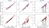 |
Fig. B.1. Comparison of physical parameters (M*, SFR, MDust) of ALPINE galaxies derived with and without the stacked IR template in CIGALE. The top and bottom panels denote the parameters derived from SED fitting assuming a Chabrier IMF and a THIMF, respectively. |
Appendix C: Schematic for estimation of optimal model parameters
In Fig. C.1, we schematize the procedure employed to estimate the optimal values of the model parameters (MGas, ini, ηin, and ϵSN). We first derive N physical parameters such as age, gas mass, SFR, and dust luminosity at 160 μm from SED fitting using CIGALE. Simultaneously, for M models (generated from a grid of h × k parameters, as taken from the gas and dust evolution, respectively), we derive M × N predicted physical parameters. We perform a reduced chi-square minimization, from which we calculate the probability (pm) for each model, where m represents an individual model, ranging from 1 to M. The mean value of each model parameter ( ) is then determined by weighting each model according to its respective probability. This procedure is discussed in detail in Sect. 3.5.
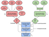 |
Fig. C.1. Visual representation of the fitting procedure presented in Sect. 3.5. The steps shaded in red denote the derivation of N physical parameters from SED fitting with CIGALE. The green steps denote the derivation of N predicted physical parameters from M chemical evolutionary models. The blue steps denote the statistical analysis used to derive the optimal value of our parameters. |
All Tables
All Figures
|
Fig. 1. Stellar mass, SFR, age, and dust mass (from top left to bottom right) plotted for galaxies assuming THIMF against Chabrier IMF. The estimates are derived from the SED fitting code CIGALE with errors calculated using a Bayesian analysis. The histograms on each axis show the distribution of the galaxies. Offsets in M*, SFR, and MDust among both IMFs are shown as ratios of the median values (and corresponding uncertainties from the 25th and 75th percentile of the distributions). The black dotted line in each panel represents the 1:1 relation. |
| In the text | |
|
Fig. 2. Age of the ALPINE galaxies as a function of sSFR assuming a Chabrier IMF (pink squares) and a THIMF (red circles). The cyan, orange, and green regions represent old (≳600 Myr), intermediate (300 − 600 Myr), and young (≲300 Myr) population of galaxies. The crossbars indicate the average error on the age and sSFR for the respective sample. |
| In the text | |
|
Fig. 3. sMGas plotted against sSFR for the ALPINE galaxies assuming a Chabrier (left) and THIMF (right). The circles represent galaxies detected via [CII], while the upper limits on gas mass are shown as inverse triangles. Evolutionary models (solid and dotted lines) are plotted for different final ages (increasing from right to left). The figure shows the case with [MGas, ini, ηout, ηin, ϵSN] ∼ [3.3, 0−2, 0.6, 0.1] and [4.4, 0−2, 0.6, 0.1] for Chabrier and THIMF, respectively. All models are color-coded by the predicted metallicity and illustrate the effect of varying ηout from 0 (solid curves) to 2 (dotted curves). |
| In the text | |
|
Fig. 4. sMDust plotted against sSFR for the ALPINE galaxies assuming a Chabrier IMF (left panel) and THIMF (right panel). The circles indicate galaxies with detected dust continuum, while inverse triangles represent upper limits on the dust mass. Dust evolution tracks are plotted for the constrained parameters [MGas, ini, ηout, ηin, ϵSN] ∼ [3.3, 0−2, 0.6, 0.1] and [4.4, 0−2, 0.6, 0.1] for the Chabrier and THIMF models, respectively, and for galaxy ages of 400 Myr, 800 Myr, and 1200 Myr for illustrative purpose. The solid color lines represent models assuming ηout = 0, while the dotted lines show the effect of increasing the outflow efficiency to ηout = 2. The models range from 25% dust condensation without dust growth in the ISM to 100% condensation with maximum dust growth efficiency. The galaxies are color-coded according to the age of their main stellar population. |
| In the text | |
|
Fig. 5. sMDust plotted against sSFR for the ALPINE galaxies assuming a Chabrier IMF (left) and THIMF (right). The circles represent galaxies with detected continuum emission, while the inverse triangles mark the upper limits on dust mass. The contributions from the various dust sources are distinguished by the different identifiers. The mass-loading factor ranges from 0 to 2. The overall dust evolution track, which includes all contributions, is shown for the constrained parameters [MGas, ini, ηout, ηin, ϵSN] ∼ [3.3, 0−2, 0.6, 0.1] and [4.4, 0−2, 0.6, 0.1] for the Chabrier and THIMF cases, respectively, at an age ∼ 1200 Myr (hatched region). The green, pink, and brown patches represent contributions from SNII, SNIa, and AGB stars, respectively. For SNII and SNIa, the models range from 25% dust condensation with ηout = 0, to 100% condensation with ηout = 2. For AGB stars, the models vary with ηout from 0 to 2. The blue patch shows the contribution of ISM growth to the total dust content, assuming a growth efficiency of 1, varying with ηout from 0 to 2. The galaxies are color-coded based on the age of their main stellar population. |
| In the text | |
|
Fig. 6. Dust-to-gas ratio plotted against sSFR for the ALPINE galaxies assuming a Chabrier IMF (left) and a THIMF (right). Only galaxies with [CII] detections are shown. The circles represent galaxies with detected dust continuum, while the upper limits on the dust mass are indicated by inverse triangles. The evolutionary models are plotted assuming [MGas, ini, ηout, ηin, ϵSN] ∼ [3.3, 0−2, 0.6, 0.1] and [4.4, 0−2, 0.6, 0.1] for Chabrier and THIMF, respectively. The models are color-coded by predicted metallicity and illustrate the impact of varying the ηout from 0 (solid curves) to 2 (dotted curves). |
| In the text | |
|
Fig. B.1. Comparison of physical parameters (M*, SFR, MDust) of ALPINE galaxies derived with and without the stacked IR template in CIGALE. The top and bottom panels denote the parameters derived from SED fitting assuming a Chabrier IMF and a THIMF, respectively. |
| In the text | |
|
Fig. C.1. Visual representation of the fitting procedure presented in Sect. 3.5. The steps shaded in red denote the derivation of N physical parameters from SED fitting with CIGALE. The green steps denote the derivation of N predicted physical parameters from M chemical evolutionary models. The blue steps denote the statistical analysis used to derive the optimal value of our parameters. |
| In the text | |
Current usage metrics show cumulative count of Article Views (full-text article views including HTML views, PDF and ePub downloads, according to the available data) and Abstracts Views on Vision4Press platform.
Data correspond to usage on the plateform after 2015. The current usage metrics is available 48-96 hours after online publication and is updated daily on week days.
Initial download of the metrics may take a while.