


| Issue |
A&A
Volume 710, June 2026
|
|
|---|---|---|
| Article Number | A305 | |
| Number of page(s) | 20 | |
| Section | Planets, planetary systems, and small bodies | |
| DOI | https://doi.org/10.1051/0004-6361/202557839 | |
| Published online | 23 June 2026 | |
Information content of JWST transmission spectroscopy of the exoplanet HAT-P-12b from the optical to the mid-infrared
1
Institute of Astronomy, KU Leuven,
Celestijnenlaan 200D,
3001
Leuven,
Belgium
2
School of GeoSciences, University of Edinburgh,
Edinburgh
EH9 3FF,
UK
3
Centre for Exoplanet Science, University of Edinburgh,
Edinburgh
EH9 3FD,
UK
4
SRON Space Research Organisation Netherlands,
Niels Bohrweg 4,
2333 CA
Leiden,
The Netherlands
5
Max-Planck-Institut für Astronomie (MPIA),
Königstuhl 17,
69117
Heidelberg,
Germany
6
Leiden Observatory, Leiden University,
PO Box 9513,
2300 RA
Leiden,
The Netherlands
7
Kapteyn Astronomical Institute, University of Groningen,
PO Box 800,
9700 AV
Groningen,
The Netherlands
8
Department of Astrophysics/IMAPP, Radboud University,
PO Box 9010,
6500 GL
Nijmegen,
The Netherlands
9
Université Paris-Saclay, Université Paris Cité,
CEA, CNRS, AIM,
91191
Gif-sur-Yvette,
France
10
School of Physics & Astronomy, Space Park Leicester, University of Leicester,
92 Corporation Road,
Leicester
LE4 5SP,
UK
11
Department of Astrophysics, University of Vienna,
Türkenschanzstr. 17,
1180
Vienna,
Austria
12
ETH Zürich, Institute for Particle Physics and Astrophysics,
Wolfgang-Pauli-Str. 27,
8093
Zürich,
Switzerland
13
STAR Institute, Université de Liège,
Allée du Six Août 19c,
4000
Liège,
Belgium
14
Centro de Astrobiología (CAB),
CSIC-INTA, ESAC Campus, Camino Bajo del Castillo s/n,
28692
Villanueva de la Cañada,
Madrid,
Spain
15
Université Paris-Saclay, CEA, IRFU,
91191
Gif-sur-Yvette,
France
16
UK Astronomy Technology Centre, Royal Observatory,
Blackford Hill,
Edinburgh
EH9 3HJ,
UK
17
Department of Astronomy, Oskar Klein Centre, Stockholm University,
106 91
Stockholm,
Sweden
18
Department of Astrophysics, American Museum of Natural History,
New York,
NY
10024,
USA
19
School of Cosmic Physics, Dublin Institute for Advanced Studies,
31 Fitzwilliam Place,
Dublin
D02 XF86,
Ireland
★ Corresponding author: This email address is being protected from spambots. You need JavaScript enabled to view it.
Received:
26
October
2025
Accepted:
2
April
2026
Abstract
Context. The James Webb Space Telescope (JWST) provides low- to medium-resolution spectra with unprecedented precision and broad near- to mid-infrared wavelength coverage, thus enabling the detailed characterization of exoplanet atmospheres. Given the complexity of JWST data and the diversity of observing modes, it is essential to understand the information content of the resulting spectra to optimize observation strategies and assess the limits of atmospheric inference.
Aims. This work presents a new JWST NIRISS SOSS transit observation of the warm sub-Saturn HAT-P-12b. Together with complementary NIRSpec G395M and MIRI LRS data, this enables a detailed assessment of the information content across JWST instruments over the full accessible wavelength range (excluding MIRI MRS).
Methods. The NIRISS data were reduced, and the impact of specific reduction choices on the resulting transmission spectrum was assessed. Atmospheric retrievals were performed for all combinations of JWST data, supplemented by archival HST observations in select cases. The analysis further included evaluations of molecular detection significances and assumptions about the atmospheric structure.
Results. The same four molecules previously reported are significantly detected: H2O, CO2, CO, and H2S. Except for H2O, all require NIRSpec coverage for detection, while H2S is only detected in multi-instrument retrievals. Abundance constraints obtained using HST WFC3 instead of JWST NIRISS SOSS are largely consistent, particularly when combining instruments, but NIRISS SOSS proved essential to establishing robust evidence for nongray cloud behavior. A moderately steep scattering slope (p < 4) is consistently retrieved across different HST STIS reductions.
Conclusions. Single-instrument retrievals, even when yielding significant detections, tend to overestimate molecular abundances. In contrast, retrievals that combine spectra from multiple JWST instruments generally converge toward consistent abundance constraints. The derived C/O ratio remains sensitive to subtle differences between NIRSpec reductions, owing to the instrument’s exclusive coverage of the carbon-bearing molecules CO2 and CO, so its interpretation requires caution. The results are broadly consistent with information content studies of the benchmark target WASP-39b, although differences, including the absence of a preference for non-isothermal T-P profiles, highlight variations in information content across exoplanet types.
Key words: methods: data analysis / techniques: spectroscopic / eclipses / planets and satellites: atmospheres / planets and satellites: gaseous planets / planets and satellites: individual: HAT-P-12b
© The Authors 2026
 Open Access article, published by EDP Sciences, under the terms of the Creative Commons Attribution License (https://creativecommons.org/licenses/by/4.0), which permits unrestricted use, distribution, and reproduction in any medium, provided the original work is properly cited.
This article is published in open access under the Subscribe to Open model. This email address is being protected from spambots. You need JavaScript enabled to view it. to support open access publication.
1 Introduction
Advances in instrumentation have enabled exoplanet science to progress from large-scale detection to the early stages of large-scale atmospheric characterization. This is exemplified by the over 300 planets1 whose atmospheres have been characterized to some extent. Because most planets cannot be observed directly, their spectral signatures must be disentangled from those of their host stars. Arguably the most important technique for doing this is transmission spectroscopy (Deming et al. 2019), which measures the wavelength dependence of the transit depth that arises in the presence of an atmosphere. Ground-based low-resolution transmission spectroscopy is feasible in the optical (e.g., Nikolov et al. 2016) and, to a limited extent, has even been applied into the infrared (IR), reaching the long-wavelength end of the near-infrared (NIR) (~2.4 μm; Crossfield et al. 2013; Danielski et al. 2014). Performing ground-based astronomical measurements further into the IR is prevented by the obstructing influence of the Earth’s atmosphere. Probing these wavelengths, however, is crucial for characterizing the chemical composition of atmospheres as most molecular rovibrational transitions occur in this region. Performing transmission spectroscopy from space can mitigate this problem. Before the James Webb Space Telescope (JWST), the primary instrument used for NIR transmission spectroscopy was the Hubble Space Telescope (HST) Wide Field Camera 3 (WFC3), mainly utilizing its G141 grism. Its 1.1 μm to 1.7 μm wavelength range enabled the detection of water from two prominent absorption bands (e.g., Iyer et al. 2016; Tsiaras et al. 2018) as well as the feature-muting effect of clouds (Sing et al. 2016; Estrela et al. 2022). Additionally, the data were useful for establishing upper limits on methane abundances (Benneke et al. 2019a; Carone et al. 2021; Edwards et al. 2023b), although the instrument mode’s narrow wavelength range and the overlapping opacity bands of water and methane led to degeneracies in the retrieved abundances of both molecules (Bézard et al. 2022). The direct detection of carbon-bearing molecules, however, remained challenging (Changeat et al. 2020; Edwards et al. 2023a). Measurements at longer wavelengths were only possible with the Spitzer Space Telescope and were mostly performed using the two photometric channels that remained operational after the end of the cryogenic mission, the Infrared Array Camera (IRAC) instrument’s 3.6 μm and 4.5 μm bands (for a review, see Deming & Knutson 2020). These were only able to provide tentative hints of possible features of molecules such as CO2 and CO (Benneke et al. 2019a; Spake et al. 2021; Alderson et al. 2022).
The advent of the JWST marked a significant advance in observational capabilities in the IR. Using a combination of instruments, spectra can be obtained with a continuous wavelength coverage from −0.6 μm to −12 μm using the Mid-Infrared Instrument (MIRI) low-resolution spectroscopy (LRS) mode, and extending to −28 μm with the MIRI medium-resolution spectrometer (MRS) (Gardner et al. 2023). The use of MIRI MRS for transmission spectroscopy has been limited to date; only a single exoplanet has been observed with this method during the first four JWST cycles (Deming et al. 2024). However, most of the other suitable JWST modes have been applied extensively for transmission spectroscopy, leading to several notable discoveries (see Espinoza & Perrin 2026, for an overview). A number of molecules, previously only detected at low significance, have now been confirmed with greater certainty, while others have been detected for the first time. These include dominant carbon species such as CO2 (Ahrer et al. 2023; Mayo et al. 2025), CO (Rustamkulov et al. 2023; Sing et al. 2024), and CH4 (Madhusudhan et al. 2023; Bell et al. 2023); the important sulfur reservoirs H2S (Thao et al. 2024) and SO2 (Alderson et al. 2023; Gressier et al. 2025); and less commonly detected molecules such as the nitrogen-bearing molecule ammonia (NH3; Welbanks et al. 2024) and even SiO (Ma et al. 2025; Gapp et al. 2025). The presence of SO2 in detectable quantities has been interpreted as the first direct evidence of photochemistry (Tsai et al. 2023). The broader wavelength coverage of JWST enables tighter constraints on cloud-induced spectral slopes, revealing evidence of complex, nongray cloud behavior (Feinstein et al. 2023; Lueber et al. 2024; Roy-Perez et al. 2025). In a few cases, features in the mid-IR have even been directly attributed to cloud particles composed of silicates (Grant et al. 2023; Dyrek et al. 2024).
HAT-P-12b (Hartman et al. 2009) is a warm sub-Saturn (Teq ~ 960K, Rp ~ 0.95RJup, Mp ~ 0.21MJup; Akeson et al. 2013, and hereafter) that has been the focus of numerous studies since its discovery. Focusing on transmission spectroscopy, the combination of the planet’s low density (ρ ~ 0.3 g cm−3), the high planet-to-star radius ratio (Rp/R* ~ 0.14), and its bright host star (K4/K5 V; mJ ~ 10.8) makes HAT-P-12b a highly suitable target for this method, as reflected by its high transmission spectroscopy metric (TSM; defined by Kempton et al. 2018) of −325 (Nikolov et al. 2022). This has led to the detection of H2O via the HST WFC3 observations, tentative hints of a possible CO2 feature from the Spitzer photometry, and the general feature-muting imprint of clouds (Wong et al. 2020). The HST Space Telescope Imaging Spectrograph (STIS) data were initially interpreted as showing a steep Rayleigh scattering slope (Sing et al. 2016), which was incompatible with previous groundbased observations indicating a flat optical spectrum (Mallonn et al. 2015). Alexoudi et al. (2018) demonstrate that a moderate steepness sub-Rayleigh slope could be inferred for both datasets when performing a consistent reduction. Subsequently obtained ground-based photometry support this interpretation (Yan et al. 2020). However, the behavior in the optical has also been interpreted as showing potential signs of stellar contamination (Jiang et al. 2021). Crouzet et al. (2025) presented the analysis of a JWST Near-Infrared Spectrograph (NIRSpec) G395M transmission spectrum which, when combined with shorter-wavelength HST WFC3 data, lead to significant detections of H2O, CO2, and CO, a non-detection of CH4, as well as a tentative detection of H2S.
This study presents the Near-Infrared Imager and Slitless Spectrograph (NIRISS) single-object slitless spectroscopy (SOSS) transmission spectrum of HAT-P-12b. This extends the spectral coverage to the shortest wavelengths accessible with JWST (−0.6 μm), beyond the range of HST WFC3 and down to the upper wavelength limit of HST STIS, probing the infrared-to-optical transition where the onset of the elusive optical slope is expected. Taken together with observations obtained using the NIRSpec bright object time-series (BOTS) mode (Crouzet et al. 2025) and with MIRI LRS (Bouwman et al., in prep.), the resulting dataset is part of a smaller subset of planets for which JWST transmission spectroscopy has been obtained over the entire feasible wavelength range (17 planets up to cycle 4, corresponding to about 12% of targets; Nikolov et al. 2022)2. not counting MIRI MRS, which has thus far seen only very limited use in the characterization of exoplanet atmospheres (Deming et al. 2024). JWST observations of the planet WASP-39b (Carter et al. 2024) have served as a benchmark dataset for assessing the information content of JWST transmission spectra (e.g., Lueber et al. 2024; Fisher et al. 2024). By evaluating various instrument combinations and testing the capabilities of JWST for a different class of exoplanet, this study contributes to a broader understanding of its capabilities across the full accessible wavelength range and multiple planetary types. The paper is structured as follows. Section 2 provides an overview of the observations used in this study. Section 3 explains how the data reduction of the NIRISS SOSS dataset was conducted. Section 4 describes the used retrieval setup. The results are presented in Sect. 5, followed by a discussion in Sect. 6, and the conclusions in Sect. 7.
2 Observations
An overview of the observations analyzed in this study is provided in Table 1. All three JWST transit spectra were obtained as part of a Guaranteed Time Observation (GTO) program of the ExoMIRI subgroup of the MIRI European Consortium (Lagage & Bouwman 2017). The NIRISS data were obtained in the NIS-RAPID readout pattern applied to the SUBSTRIP256 subarray using 15 groups per integration. The total observation time was −6.2 hours which corresponds to 254 integrations. This covered the −2.3 hour transit along with a stellar baseline of −2.4 hours before ingress and −1.4 hours after egress. No additional exposure using the F277W filter was obtained. By restricting the aperture position angle, any major contaminations could be avoided, rendering such an exposure noncritical. Details on the NIRSpec and MIRI data and their reductions are provided in Crouzet et al. (2025) and Bouwman et al. (in prep.). This study primarily uses the reductions obtained with CASCADe, while the TEATRO reduction of the NIRSpec data is employed for additional robustness tests.
In select cases, HST data were also included for further analysis. The spatial scanning mode HST WFC3 data first presented by Tsiaras et al. (2018) was used. As in the other papers of this series, this study uses the CASCADe reanalysis of the data (see Crouzet et al. 2025 for details). In addition, HST STIS data were used to provide information further into the optical. No reanalysis of the data was performed. Instead, the impact of the two distinct reductions presented in Sing et al. (2016) and Alexoudi et al. (2018) were tested.
Key properties of the observations and resulting transmission spectra.
3 NIRISS data reduction
The reduction of transmission spectroscopy data requires transforming raw detector readouts into calibrated spectra and fitting the resulting transit light curves to derive the transit spectrum. Several methodological choices in this process can significantly affect the inferred atmospheric properties (Mugnai et al. 2024). As the true planetary signal cannot be directly observed, it is often unclear which reduction approach most faithfully recovers it. Even seemingly minor differences in the resulting transmission spectrum can impact the inferred atmospheric composition (e.g., Crouzet et al. 2025). One commonly adopted approach to test the robustness of the obtained transmission spectra is to perform multiple independent data reductions using different pipelines (e.g., Feinstein et al. 2023; Rustamkulov et al. 2023; Radica et al. 2023). This paper presents an analysis similar to that of Holmberg & Madhusudhan (2023), focusing on the effect of individual “tweaks” to the data reduction. Rather than comparing sets of multiple tweaks, as is effectively done when comparing outcomes of different pipelines, the emphasis here is on isolating the impact of specific steps. The following two sections describe the choices that define the standard reduction, i.e., the reduction used in the subsequent retrieval analysis. During the first part of the data reduction, the light curve extraction, the choices made mostly followed the default methods of the used pipeline. In the second part of the reduction, an approach similar to that applied to the other two datasets (Crouzet et al. 2025; Bouwman et al., in prep.) was adopted, and simplifying assumptions were made whenever applicable. The applied tweaks and their impacts are described and discussed in Appendix B.
3.1 Light curve extraction
The ExoTEDRF pipeline3 (formerly known as supreme-SPOON; Radica 2024) was used to obtain spectral light curves from the uncalibrated group-level images. The pipeline was initially developed to deal with the unique peculiarities of the NIRISS SOSS mode. These include the presence of multiple spectral orders and the nonconstant background with its distinct “step” caused by dispersed zodiacal light. It has been used for NIRISS SOSS transit spectroscopy observations of multiple targets and was also benchmarked against other pipelines (e.g., Radica et al. 2023; Feinstein et al. 2023).
The data reduction started out from uncalibrated data produced by version 2023_1a of the JWST Science Data Processing (SDP) system. These are then processed using version 2.0.0 of the ExoTEDRF pipeline. It leverages the standard jwst pipeline for many of the common reduction steps. Version 1.12.5 (Bushouse et al. 2023) of the jwst pipeline was used, which is the version recommended for the used version of ExoTE-DRF. No further refinements were applied to the reference files, which were obtained with the Calibration Reference Data System (CRDS; Greenfield & Miller 2016) using context 1290. The context version was fixed to ensure a consistent comparison between the different reduction tweaks. Some of the custom ExoTEDRF steps do require additional observation-specific reference files. While these can be estimated dynamically during pipeline execution, more accurate results are typically obtained by first running the full pipeline in a first pass and generating the reference files from the output. This two-pass approach was therefore adopted here. The setup adopted for the standard reduction closely followed that of Radica et al. (2023), with one key difference: The OneOverF step was applied not only at the group level but also at the subsequent integration level. Applying the correction at the integration level alone is a commonly adopted approach in NIRISS reductions with other pipelines (e.g., Feinstein et al. 2023). The correction was applied at both stages in the standard reduction to account for the possibility of residual 1/f noise persisting at the integration level after the group-level correction, and to define a consistent baseline against which tweaked reductions, where the correction was only applied in a single stage, can be directly compared. Technical details regarding the pipeline’s implementation can be found in the official documentation4. The ExoTEDRF pipeline can be configured via a YAML configuration file. The file used in the standard reduction is publicly available (see Data availability).
During the first two stages, calibrations and corrections are applied to the data, first at the group level and then, after fitting the integration “ramps” to the resulting integration-level images. The NIRISS background consists of at least two distinct components: the true sky background, primarily composed of dispersed zodiacal light, which enters the detector due to the slitless design of the spectrograph, and the so-called “1/f noise”. The latter is a form of correlated detector readout noise that affects all JWST NIR detectors to some extent (Schlawin et al. 2020). Since the 1/f noise is much weaker than the sky background, the latter must be removed first. In principle, the 1/f noise also varies from group to group and should therefore be removed during the first stage. The sky background on the other hand is best removed later in the second stage close to the spectral extraction. In the reduction approach presented in Radica et al. (2023) this is done by temporarily removing an estimate of the sky background in the first stage to reveal the remaining 1/ f noise. This noise is then estimated on a column-by-column basis and removed. The sky background gets re-added and then again estimated and subtracted, this time permanently, in the second stage. The present work modified this approach for the standard reduction by introducing an additional subtraction of a column-specific noise signal in the second stage. To estimate the sky background, a background model was scaled to the flux level of a median stack of all out-of-transit images, computed either per group or as a single stack at the integration level. The background model used was obtained during commissioning (formerly listed on JDox; observation 5 of program ID 1541)5. The default ExoTEDRF method applied in the standard reduction determines the scaling factor using a single rectangular low-flux region. The default positioning of this region was confirmed to be adequate (x1 ∈ [350,549], y1 ∈ [230, 249]; see Fig. B.2). To estimate the 1/f noise, ExoTEDRF provides four built-in methods. In the standard reduction, the default and simplest one, scale-achromatic, was used. It scales the median-stack images to the estimated flux level of each group or integration image. As the name suggests, the scaling is performed achromatically using a white light curve estimate derived from the first pass reduction.
In the third stage, a single step is executed to extract a timeseries of spectra from the corrected and calibrated integration images. Flux extraction was performed with a simple box extraction using the default aperture width of 35 pixels, close to the “optimal” value of 36 determined by the pipeline’s optimization routine, which selects the aperture width that minimizes white light curve scatter. For determining the trace positions, the optional reference file from the first pass reduction was used. The ExoTEDRF implementation of the spectral extraction step includes an optional wavelength calibration based on theoretical PHOENIX stellar atmosphere models (Husser et al. 2013). This calibration was applied using stellar parameters ( , log g*, [Fe/H]) taken from Mancini et al. (2018, see also Table A.1 in this work).
3.2 Light curve fitting
Although the ExoTEDRF pipeline (Radica 2024) provides built-in tooling for performing spectral light curve fits on its stage 3 output, a custom script based on the same underlying exoplanet system modeling tool, juliet (Espinoza et al. 2019), was used instead. This was done to allow for greater flexibility in the chosen fitting approach. The scripts used to perform the fitting are publicly available (see Data availability). Overall, an approach similar to that utilized for the TEATRO reductions of the other two HAT-P-12b JWST datasets (Crouzet et al. 2025; Bouwman et al., in prep.) was adopted in the standard reduction.
Following well-established methodology (e.g., Stevenson et al. 2014; Kreidberg et al. 2015), the data are first fitted achromatically using so-called white light curves. Two white light curves were constructed. The first was derived from the full wavelength range of the first spectral order (0.85 μm to 2.83 μm). The second white light curve was derived from the second spectral order, which nominally spans approximately 0.59 μm to 1.41 μm. However, the data at both ends of this range are too noisy and were therefore excluded from further analysis. In addition, the longer-wavelength part of the second order overlaps with the first order, which provides a significantly higher throughput (up to a factor of ~500 at 1.27 μm). For these reasons, only a restricted wavelength range of 0.6 μm to 0.85 μm was used for the second-order white light curve. The resulting light curves were normalized by the mean out-of-transit baseline flux. The first integration was excluded from the baseline normalization and subsequent fitting, as it is clearly identifiable as an outlier (see Fig. 1); no binning in the temporal domain was applied. Both light curves were fitted simultaneously using a single combined model that shares the same orbital parameters. Either wide uninformative priors or Gaussian priors based on previous literature findings were used. The full set of used parameters, including priors and posterior values are listed in Table A.1. There are several possible parametrizations of the orbit available (Espinoza et al. 2019). Here, a parametrization based on the orbital period P, transit mid-time t0, scaled semimajor axis a/R*, impact parameter b, eccentricity e, and argument of periastron ω was adopted. The orbital period was fixed to the literature value reported by Kokori et al. (2022). A circular orbit was assumed, fixing the eccentricity to e = 0 (consistent with the 1σ upper limit e < 0.035 reported by Bonomo et al. 2017). In this case, the argument of periastron is undefined and was therefore arbitrarily fixed to ω = 90°. The two white light curves are constructed by binning the timeseries of spectra over distinct wavelength ranges, resulting in variations in transit shape due to the wavelength dependence of both the transit depth and limb darkening. Both effects therefore need to be treated separately for each spectral order. For the former, this implies fitting two independent transit depths δ. Limb darkening was likewise freely fitted for to account for known degeneracies with orbital parameters that also influence the transit shape, such as the impact parameter b (Espinoza & Jordán 2015). Specifically, a quadratic law was adopted. The limb darkening coefficients (LDCs) u1 and u2 were permitted to vary freely (hereafter referred to as “free”) within the physically informed reparametrization proposed by Kipping (2013), expressed in terms of the transformed parameters q1 and q2. The baseline was assumed to be flat. The juliet transit light curve model also includes several orderspecific systematic parameters, namely the dilution factor D, the relative out-of-transit flux M, and a jitter term σω. The dilution factor was fixed at 1 (no contamination), while the other two parameters were allowed to vary freely within wide uninformative priors. Together with these additional systematic parameters, a total of 13 parameters were fitted. The juliet code supports several different samplers. In this work, the dynesty sampler (Speagle 2020), a commonly adopted choice (e.g., Pontoppidan et al. 2022; Fournier-Tondreau et al. 2024), was employed with the number of live points set to 5000.
To obtain the final product of the data reduction, the transmission spectrum, the spectral light curves first need to be fitted. Following the approach of Radica et al. (2023), the data were rebinned to a spectral resolution of R ~ 125. The bins correspond to full pixel ranges without interpixel interpolation (order 1: 423 pixels, order 2: 6-15 pixels), resulting in slight variations in pectral resolution between bins (see Table 1). The second spectral order was restricted to the same range as for the white light curve. As in the case of the white light curves, the first integration was discarded and no temporal binning was applied. The orbital parameters were fixed to the values from the white light curve fit (see Table A.1). Since the aforementioned degeneracy between these parameters and the LDCs is therefore resolved, and given the much reduced S/N of the spectral light curves when compared to the white light curves, the LDCs were fixed to values predicted by stellar atmosphere models (hereafter referred to as “fixed”) instead of freely fitted for. For this purpose, the ExoTiC-LD Python package (Grant & Wakeford 2024), together with the Stagger model grid (Magic et al. 2015), was used with the order-specific throughput data from the CRDS NIRISS reference file, evaluated over the wavelength range of each spectral bin. This leaves a total of three parameters (Rp/R*, M, σω) to be fitted separately for each spectral bin. Reflecting the reduced model complexity and lower S/N of the spectral bins, the number of live points was reduced to 500. Finally, the transmission spectrum was obtained by transforming the marginal posterior of Rp/R* into a posterior of the transit depth δ, adopting the posterior median as the nominal value and the standard deviation as the uncertainty. The resulting transmission spectrum is publicly available (see Data availability).
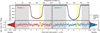 |
Fig. 1 White light curves created from the first two spectral orders of the NIRISS SOSS data and combined best-fit model. The top panels show the observed data and fitted model light curves, while the bottom panels show the standardized residuals. The standardized residuals are the residuals divided by the uncertainty σφ that combines the uncertainties in flux reported by the pipeline σt with the additional jitter term σω fitted by the juliet framework ( |

4 Retrievals
The transmission spectra were fitted using the forward modeling and retrieval framework ARCiS6. It offers a high degree of flexibility, supporting a wide range of modeling complexities (Min et al. 2020). The code has been extensively tested and benchmarked against other atmospheric retrieval frameworks (Barstow et al. 2022). The general setup closely follows that of the two companion studies (Crouzet et al. 2025; Bouwman et al., in prep.). Values from Mancini et al. (2018) were adopted for the system parameters (R*, T*, d, a, Mp; see Table A.1). The reference pressure Pref, the pressure level that corresponds to the retrieved planetary radius, was fixed at 10 bar. The atmospheric structure was modeled using 100 layers equidistant in logspace, spanning the range of [102,10−10] bar. The atmospheric structure was chosen to reflect the complexity of JWST data through an N-point profile of five temperature points Tp,i, evenly spaced in log-pressure over the full modeled pressure range. A smoothing window, averaging over about nine adjacent pressure points (|log(Pi/Pj)| ≤ 0.6), yields the final T-P profile. Given the planet’s low density, a primordial atmosphere was assumed, i.e., one primarily composed of a background gas mixture of hydrogen and helium at solar-like abundance ratios (H2/He = 0.85/0.15 ≈ 5.7; cf. ≈ 6.1 in Asplund et al. 2021). The effects of the background gas molecules on the transmission spectrum were included through their contributions to Rayleigh scattering and collision-induced absorption (CIA). For the latter, HITRAN data (Karman et al. 2019) were used, including CIA from H2-H2 (combined from Abel et al. 2011; Fletcher et al. 2018) and H2-He (Abel et al. 2012) collisions. The abundances of all molecular and atomic trace species are parametrized as logarithmic volume mixing ratios (VMRs), Xx = nx/ntotal, and were assumed to be vertically constant throughout the atmosphere (isochemical), a common simplification in atmospheric retrievals (e.g., Madhusudhan 2019; Lueber et al. 2024). Their contribution to the transmission spectrum was modeled using opacities from the ExoMol database (Tennyson & Yurchenko 2012) provided as correlated k-tables (Chubb et al. 2021). The used set of molecules included those previously detected for this planet, i.e., H2O (linelist: Polyansky et al. 2018), CO2 (Yurchenko et al. 2020), CO (Li et al. 2015), and H2S (Azzam et al. 2016). Additionally, species that have been identified in JWST transmission spectra of other exoplanets (see Sect. 1), namely CH4 (Yurchenko et al. 2024), SO2 (Underwood et al. 2016), and the potential nitrogen reservoirs NH3 (Coles et al. 2019) and HCN (Barber et al. 2014), were included as well. Finally, the potential impact of clouds was modeled using a nongray cloud parametrization. It assumes a simple, homogeneous cloud structure, which effectively fills the atmosphere below a certain upper pressure limit Pcloud with cloud particles of constant mixing ratio Xcloud, combined with a parametrized opacity κcloud for the cloud component,
 (1)
(1)
which mimics the expected behavior of physical cloud particles by reaching a constant reference opacity κ0 at short wavelengths λ < λ0 and following a wavelength-dependent power-law of steepness p at longer wavelengths, implying a cloud opacity in the optical that can be at most as steep as in the IR and may flatten toward shorter wavelengths.
The retrievals were carried out using the ARCiS interface to the MultiNest code (Feroz & Hobson 2008; Feroz et al. 2009, 2019). Nested sampling was performed with 2500 live points and an efficiency rate of 0.3. The planetary radius, the five temperature points, the chemical abundances of the included species, and the parameters of the cloud model were treated as free parameters. Since the cloud particle mixing ratio Xcloud and reference opacity κ0 are exactly degenerate, only the former was varied, while the latter was arbitrarily fixed to 1000 cm2 g−1. The only quantity that can be constrained is the product of these two parameters. The retrievals also allowed for a variable offset Δδ0,z between observations from different instruments. The offsets were included as additional free parameters (n – 1 parameters for n instruments) sampled within the nested sampling framework. In general, wide and uninformative priors were chosen (see Table 2). The prior for the spectral slope was specified to permit shapes ranging from flat to super-Rayleigh.
Using the general setup described above, a number of different retrievals were performed. First, and forming the core of this study, seven retrievals using all possible combinations of the JWST instruments NIRISS, NIRSpec, and MIRI were conducted. To specifically assess the benefits of the NIRISS SOSS mode, four retrievals were performed in which it was replaced by the overlapping but narrower and lower signal-to-noise (S/N) HST WFC3 mode. Finally, to test the impact of the JWST data, especially NIRISS SOSS, on the retrieved slope in the optical, combined retrievals with different reductions of the STIS data were performed. For these retrievals, instrumental transit depth offsets were optimized separately using a least-squares minimization, following earlier work in this series (Crouzet et al. 2025), as including additional offset parameters directly in the nested sampling for the full STIS+JWST combinations would be computationally prohibitive. Tests for other multi-instrument combinations showed that this choice results only in minor differences in the resulting posterior (see Appendix C.1). Also, opacities of the atomic species sodium (Na; Allard et al. 2019) and potassium (K; Allard et al. 2016) were additionally included. To quantify detection significances of the included molecules, additional “leave-one-out” retrievals were conducted. Further, retrievals were performed using a gray instead of a nongray cloud parametrization, and an isothermal in place of the standard N-point T-P profile, to assess the impact of these modeling assumptions. The influence of cloud opacity was also tested by fixing the spectral slope parameter to p = 0.
Priors used in the retrievals conducted in this study.
5 Results
5.1 NIRISS data reduction
The white light curve fits of the NIRISS SOSS data (see Fig. 1) show generally good agreement between the data and the best-fit model, with a reduced chi-square of  and root mean square (RMS) residuals of 114 ppm for order 1 and 189 ppm for order 2. A localized deviation is observed in both light curves starting approximately 25 minutes after mid-transit and lasting for about 25 minutes (nint ∈ [164,179] ). This feature may be attributable to a spot crossing event. The impact of such events was explicitly tested using tweaked reductions (see Appendix B.1). Differences in the resulting transmission spectrum are found to be minor (see Appendix B.2), and therefore the simpler spotless modeling was retained for the standard reduction. While the one-dimensional distribution of standardized residuals closely follows the expected Gaussian shape (p ≫ 0.05 for skewness and kurtosis tests), the time-resolved residuals still exhibit structured deviations. The spectral light curves also generally show good agreement when accounting for the reduced S/N when compared to the white light curves (
 ~ 1.2-2.5, RMS ~ 400-2000 ppm; see Fig. A.2 for representative example light curves). While a direct comparison between the LDCs freely fitted for in the case of the white light curves and the fixed model values adopted for the spectral light curves is limited by their differing wavelength ranges, systematic differences are apparent. Specifically, the fitted LDCs tend to favor higher values of u1 and lower values of u2 than the corresponding model values. These differences were further investigated using additional tweaked reductions (see Appendix B.1 and Fig. B.3). Accounting for an offset of 250 ppm in the transit depth (well within the adopted prior range of 1000 ppm), which was treated as a free parameter in the retrievals, brings the NIRISS transmission spectrum into good agreement with the HST WFC3 spectrum at overlapping wavelengths (see Fig. A.1).
5.2 Retrievals
To interpret the retrieval results, individual molecular bands were identified using the database by Crovisier (2002). The corresponding opacity contributions of the different species are shown in Fig. 2. Frequentist nσ detection significances were derived from differences in Bayesian log-evidence Δ ln Z using the method from Sellke et al. (2001); Trotta (2008). While this approach is commonly used in atmospheric retrieval studies (e.g., Benneke & Seager 2013; Kreidberg et al. 2015; Edwards et al. 2023b), the obtained detection significances should be treated with caution (Kipping & Benneke 2025; Welbanks et al. 2026). The results from the three sets of retrievals are discussed separately in the following sections.
5.2.1 JWST instrument combinations
Significant detections (>3σ) are achieved for four molecules: H2O, CO2, CO, and H2S (see Fig. 3). These are the same species found in Crouzet et al. (2025). Any combination of instruments involving NIRISS leads to a highly significant detection of H2O. Even for NIRISS alone the significance is above 12σ. The reason for this is the coverage of numerous dominant and well-isolated absorption bands. A detection without NIRISS requires combining NIRSpec and MIRI. NIRSpec captures only the long-wavelength tail of the fundamental stretching bands (ν1 and ν3), with the rest of its range dominated by other molecular features.
In contrast, MIRI is limited by lower S/N, a consequence of the declining stellar flux in the mid-IR. This combination yields a detection significance of ~8σ, which drastically increases to ~15σ when NIRISS is included as well. A significant detection of CO2 is only possible when NIRSpec data is included, yielding very high significances of >10σ. This is due to the strong and well-isolated asymmetric stretch band ν3 at ~4.3 μm falling within NIRSpec’s range. For CO, instrument combinations that include NIRSpec reach ~5σ, probably due to the fundamental band at ~4.7 μm. Notably, NIRSpec alone does not enable a significant CO detection, as the retrieval can match the observed opacity using only H2 O and CO2. However, as shown by Crouzet et al. (2025), the alternative TEATRO reduction can produce substantially higher detection significances, indicating that the result remains sensitive to the data reduction approach. A significant detection of H2S is only possible when NIRSpec data are included, due to its symmetric stretch band ν1 near 3.8 μm, which lies in a spectral region where H2O and CO2 opacity reaches a local minimum. Using NIRSpec alone yields a lower significance of ~3.1σ, while combinations with other instruments generally achieve >4.9σ. The H2S opacity in this region could also be mimicked by gray cloud opacity, but added constraints from NIRISS and MIRI help break this degeneracy, enabling a more robust detection. This effect is also observed in Crouzet et al. (2025), where H2S is only detected for the CASCADe reduction. To test whether the TEATRO reduction also yields a detection of H2S when combined with the other JWST data, an additional retrieval was performed. The resulting detection significance is lower at ~3.7σ, but remains significant.
Significant detections correspond to narrow, well-constrained posteriors, whereas non-detections yield broad distributions with only upper limits and extended tails toward lower abundances (except for H2O with MIRI; see Fig. 4 and Table C.1). For molecules with significant detections, the posteriors are mostly consistent within their 1σ intervals. Combining several instruments often leads to consistent but more tightly constrained abundances compared to single instruments. Notable outliers are the abundance constraints for H2O with NIRISS and CO2 with NIRSpec, both yielding significantly higher values. This underscores the need for broad wavelength coverage to constrain the atmospheric structure, since retrievals based on limited data can yield precise but biased posteriors. For molecules without significant detections, combining instruments still proves beneficial, typically leading to tighter 95th percentile upper limits on their abundances. For CH4, most upper limits cluster around −6 dex, with slightly higher values for the NIRISS and NIRSpec+MIRI retrievals, the latter even showing a pronounced peak at the upper bound. For SO2, the upper limits fall into distinct tiers. The NIRISS-only retrieval yields the loosest constraint at approximately −3.3 dex, approximately 3 dex higher than all others. This is not surprising since both NIRSpec and MIRI have regions with dominant SO2 absorption bands while NIRISS does not. Retrievals including only MIRI or NIRISS+MIRI exhibit peaks at the upper limit, but the peak disappears when more instruments are included.
The most stringent limits are obtained when both NIRSpec and MIRI are included (either with or without NIRISS), lowering the upper limit by ~0.2 dex compared to other combinations. For NH3, upper limits again generally tighten as more instruments are added. MIRI has the largest impact, probably due to strong, broad absorption beyond ~9 μm from the molecule’s symmetric bend “umbrella” mode ν2, followed by NIRSpec, while NIRISS contributes the least. For HCN, two groups of constraints can be distinguished. Retrievals that exclude NIRSpec yield significantly looser limits. Including NIRSpec lowers the upper limit by more than 2.2 dex, most likely because its wavelength range covers both the fundamental C-H stretch ν3 at ~3.0 μm and the combination band of C-N stretch and the bend mode ν1 + ν2 at ~3.6 μm.
In addition to the tests on molecular detection significance, significance tests of key atmospheric assumptions, such as the choice between sloped nongray and flat gray cloud opacities, were also performed (see Fig. 3). A preference for the sloped model is only significant, at more than ~7.5σ, when the NIRISS data is included. This is expected, since the effect of the spectral slope becomes more pronounced at short wavelengths. Additionally, there is a dip in transit spectrum around 2.3 μm between two H2O bands which cannot be adequately reproduced by a gray cloud model (see Fig. 2). Such a feature is also observed in Feinstein et al. (2023), where it is interpreted as an indication of a nongray cloud opacity and in their case even inhomogeneous cloud coverage. Figure 5 shows marginal and joint posteriors of the cloud parameters for select instrument combinations. The joint distributions reveal notable correlations between several parameters. Retrievals using only NIRSpec and MIRI, whether individually or combined, yield flat posteriors matching the priors. In contrast, combinations including NIRISS provide clear constraints. The cloud particle mixing ratio Xcloud is constrained to be above −4.4 dex. The cloud-top pressure Pcloud is generally constrained to be lower than 10−3′6 bar, requiring the cloud to extend into the probed layers. The reference wavelength λ0 is limited to be below 2 μm for NIRISS+MIRI and below 1.5 μm for the remaining combinations, matching the shape of the NIRISS spectrum at short wavelengths. Finally, all NIRISS retrievals also favor sub-Rayleigh slopes with p < 4, except for NIRISS+NIRSpec, where a super-Rayleigh slope with p > 4 is preferred above the 32nd percentile. No significant preference for the more complex N-point profile over the isothermal temperature profile is found. The information content of the data therefore does not justify the added complexity introduced by a non-isothermal profile. For the combination of all three instruments, the use of a complex profile has negligible impact in the pressure range between 1 × 10⁻⁵ bar to 1 × 10⁻³ bar (see Fig. 5), which is the region typically probed by transmission spectroscopy. Outside this range, the median N -point profile deviates noticeably from the isothermal profile, but remains poorly constrained.
Overall, these results might give the impression that MIRI generally provides little additional benefit compared to NIRISS and NIRSpec. However, this largely reflects the characteristics of this particular planet, as it does not exhibit any strong MIRI-specific features (e.g., SO2 and silicate clouds; Dyrek et al. 2024).
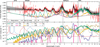 |
Fig. 2 Visualization of the HAT-P-12b transmission spectrum and the underlying opacity contributions. The top panel shows combined spectra from the three JWST instruments and HST STIS (Alexoudi et al. 2020) with 1σ uncertainties, together with the best-fit model with its 3σ credible interval. Model spectra including only the opacity of individual contributors (chemical species or cloud parametrization) are also shown. The bottom panel shows absorption cross sections (σ) of all tested chemical species. Significantly detected species are emphasized with thicker lines. |
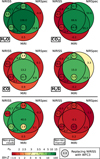 |
Fig. 3 Venn diagrams of JWST instrument combinations showing detection significances of the four significantly detected molecules (top) and the preference for two modeling assumptions (bottom). Additional circles show the significances obtained when replacing the JWST NIRISS SOSS with the HST WFC3 instrument data. The significances are reported as log-evidence differences ∆ ln Z and visualized using a custom nonlinear color scale. The color bar also provides a conversion to nσ detection significances following the calibration scale from Benneke & Seager (2013). |
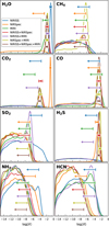 |
Fig. 4 Marginal posterior distributions of the chemical abundances for all included molecules, retrieved using different JWST instrument combinations. The shown distributions were derived from the samples via kernel density estimation (Gaussian kernel with bandwidth h = 0.1). For each distribution, the markers indicate either the 1σ credible interval for well-constrained posteriors or the 95th percentile upper limit (arrows) when only an upper bound can be established. |
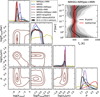 |
Fig. 5 On the left, an excerpt of the corner plot focusing on parameters of the cloud parametrization is shown. The joint posterior distributions (off-diagonal panels) are only shown for the retrieval using all JWST instruments and are visualized using contour lines smoothed with a Gaussian kernel (σ = 1). The marginal posterior distributions (diagonal panels) are additionally shown for exemplary JWST instrument combinations, as well as the results from retrievals that include the two HST STIS reductions. The same kernel density estimation as in Fig. 4 was applied. Additionally, in the upper right, a comparison of T-P profiles derived for the more complex N-point and the simpler isothermal parametrizations for the case of the three JWST instrument combination is shown. The lines indicate the median value, while the shaded regions are used to highlight the [0.5, 1,2,3] σ credible intervals. |
5.2.2 NIRISS versus WFC3
The retrievals using HST WFC3 instead of NIRISS SOSS show that most molecules significantly detected with NIRISS are also detected with WFC3 (see Fig. 3). A notable exception is CO, for which a significant detection only occurs when WFC3 is combined with NIRSpec and MIRI. This is probably due to the limited wavelength coverage of WFC3, which excludes the strongest CO absorption band in the NIRISS range, the first overtone (Δν = 2) near 2.3 μm. To quantify changes in the marginal posterior distributions, the difference between the median values for bounded constraints or the upper 95th percentile for upper limits is calculated. These are reported both in dex and in units of σ, where σ is the combined 1σ uncertainty of the two distributions, obtained by adding their individual 1σ uncertainties in quadrature (dexlσ shorthand is used when values in dex and σ are identical). Differences in the retrieved chemical abundances are generally small for multi-instrument combinations (≲0.7 dex|σ; see Fig. C.1), a notable outlier being the CO2 abundance for WFC3+NIRSpec (1.4 dex, 1.7σ). The difference becomes negligible (0.03 dex, 0.05σ) once MIRI is included as well. For single-instrument retrievals, however, the results can be substantially more discrepant. H2O is the only molecule significantly detected with WFC3 alone; instead of a narrow, well-constrained posterior, a distinctly different (2.5 dex, 1.9σ) bimodal distribution is retrieved. For most other molecules, except for CO2 and CO (≲0.28 dex, ≲0.05σ), the upper limits differ considerably between the single-instrument retrievals (≲2.8 dex, ≲0.6σ). For CH4, H2S, NH3, and HCN, WFC3 yields lower upper abundance limits than NIRISS, highlighting the risk of overconfident interpretations from WFC3 data alone.
In the case of HAT-P-12b, both WFC3- and NIRISS-only retrievals attribute their common spectral features to water.
However, the WFC3 G141 grism covers only a single full H2O band, making it susceptible to confusion with other molecules, particularly with CH4, which has a similar although narrower and slightly shifted feature. An example for this confusion is K2-18b (H2O: Benneke et al. 2019b; Tsiaras et al. 2019; CH4: Bézard et al. 2022; Madhusudhan et al. 2023).
While differences in molecular detections and abundance constraints are mostly negligible when several instruments are combined, NIRISS and WFC3 markedly differ in their ability to constrain the cloud opacity. With NIRISS, a strong preference for nongray clouds is found both in the single instrument retrieval and in any combination with other instruments (≳7.5σ). In contrast, WFC3 alone does not yield significant evidence. Only the WFC3+MIRI combination, a combination with a significant 3 μm wavelength gap, shows a clear preference (4.2σ), which weakens to tentative levels (2.9σ) once NIRSpec is also included.
5.2.3 Inclusion of STIS data
By combining the disparate STIS spectra from Sing et al. (2016, hereafter “Sing2016”) and Alexoudi et al. (2018, hereafter “Alex-oudi2018”) in separate, dedicated retrievals with the JWST data, especially NIRISS, it can be tested whether the retrieved steepness of the slope is still affected by differences between the STIS datasets. Given the dominance of the cloud opacity at optical wavelengths, it is unsurprising that the retrieved chemical abundances are only marginally affected (≲0.27 dexlσ) by the inclusion of STIS data. The additional atomic species of sodium and potassium are not detected, whether the STIS data are included or not. For potassium, the retrievals produce very similar posteriors, with 95th percentile upper limits around −6.6 ± 0.1 dex. Sodium shows slightly higher limits without STIS, peaking near −2.7 dex, and lower limits with STIS around −3.75 ± 0.25 dex.
The cloud parametrization is more strongly impacted (see Fig. 5). All parameters, except for the cloud-top pressure Pcloud, are significantly affected. In particular, the retrieved spectral slope p shifts to lower values when STIS data are included alongside the JWST observations (JWST+Sing2016:  ; JWST+Alexoudi2018:
  ) compared to the retrieval using JWST data alone (
 ). A preference for sub-Rayleigh slopes (p < 4), i.e., up to the upper uncertainty bounds, is therefore only obtained when STIS data are included, while differences between the two STIS datasets themselves have little impact. It should be noted, however, that the adopted cloud parametrization does not allow for an optical slope steeper than at longer IR wavelengths. This coupling may limit the ability of the retrievals to reproduce Rayleigh-like scattering behavior in the optical. Nevertheless, both STIS-inclusive cases show a stronger preference for sub-Rayleigh slopes than the JWST-only retrieval.
6 Discussion
6.1 Elemental composition
Molecular abundances inferred from transmission spectra can be used to estimate elemental abundance ratios, such as the carbon-to-oxygen (C/O) ratio and metallicity. These quantities are of particular interest because they can be compared to solar system mass-metallicity trends (Thorngren et al. 2016; Welbanks et al. 2019) and may provide insights into planetary formation and migration processes (Öberg et al. 2011; Mordasini et al. 2016; Thorngren & Fortney 2019; Mollière et al. 2022; Khorshid et al. 2024).
The weighted retrieval samples were used to derive C/O ratios and metallicities for the various JWST instrument combinations. All molecules, detected or not, were included in the calculation, such that undetected molecules still contributed to the overall uncertainty. For the metallicity Z, the ratio of carbon and oxygen to hydrogen was used as a proxy, since the other two atomic species, sulfur and nitrogen, are not as reliably constrained. All retrievals generally favor supersolar metallicities (see Fig. 6). Single instrument retrievals, however, prove less reliable. For NIRISS and NIRSpec, the aforementioned overestimation of H2O or CO2 results in metallicities around ~100× solar, well above the ~10× solar inferred from most combination retrievals.
Given the strong influence of the NIRSpec data on the inferred abundances of carbon-bearing species, an additional retrieval was performed using the full JWST dataset, replacing the CASCADe NIRSpec reduction with the TEATRO reduction (Crouzet et al. 2025). The impact on metallicity is minimal, the C/O ratio, however, is more strongly impacted (values given below). This can be attributed to shifts in the molecular abundances. While these all stay within their 1σ uncertainty intervals, the ratio of H2O/CO drops by more than half, while CO/CO2 nearly doubles. The retrievals based on CASCADe yield C/O ratios broadly consistent with the stellar value, with a preference for substellar values. In contrast, the TEATRO-based retrieval favors a wider range from stellar to solar values, a difference already noted in Crouzet et al. (2025) although using the WFC3+NIRSpec combination instead of NIRISS+NIRSpec+MIRI.
The values inferred from the retrievals including all JWST instruments are C/O =  and Z =
  for CASCADe, and C/O =
  and Z =
  for TEATRO. These results are broadly consistent with previous results from Crouzet et al. (2025), despite differences in the retrieval setups. Pre-JWST results based on HST, Spitzer, and ground-based photometry and made under the assumption of equilibrium chemistry typically found near-solar C/O ratios, but are still compatible with subsolar values (Wong et al. 2020; Yan et al. 2020; Panek et al. 2023). Metallicities varied widely, from notably lower values (< 10× solar; Yan et al. 2020; Panek et al. 2023) to much higher estimates (> 100× solar; Wong et al. 2020; Jiang et al. 2021). These comparisons underscore the importance of JWST’s broad spectral coverage and precision for obtaining robust, though potentially still reduction- and model-dependent, estimates of elemental abundances.
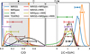 |
Fig. 6 Marginal posterior distributions of the C/O ratio and metallicity ([(C+O)/H]) derived from molecular abundances for all JWST instrument combinations. An additional retrieval of all JWST instruments using the NIRSpec TEATRO instead of the standard CASCADe reduction is also shown (labeled TEATRO). The interval markers follow the convention introduced in Fig. 4. Solar (⊙; Asplund et al. 2021) and stellar (★; Biazzo et al. 2022) values are indicated on the top axis. The gray shading marks the uncertainty in the stellar values. |
6.2 Behavior in the optical
As discussed in detail in the introduction, there have been discrepant results regarding the shape of the transmission spectrum of HAT-P-12b at optical wavelengths. Combining either of the disparate STIS data reductions with the JWST data from all three instruments results in a clear preference for a shallow slope, which is very different from the results obtained when analyzing the STIS data on its own (Alexoudi et al. 2018). As discussed in Sects. 4 and 5.2.3, the adopted cloud parametrization intrinsically limits the optical cloud opacity to be at most as steep as at longer IR wavelengths. While this physically motivated assumption provides a compact description across the full wavelength range, alternative cloud opacity treatments will be explored for the JWST data in future work (Bouwman et al., in prep.). The preference for a shallow optical slope may be further reinforced by the greater weight of the JWST data in the retrievals, as their smaller uncertainties and higher number of data points compared to the STIS data lead the sampling algorithm to favor them. Given the importance of the NIRISS data when it comes to constraining the shape of the spectral slope, as illustrated by its necessity to obtain a significant preference for the nongray cloud parametrization (see Fig. 3), ensuring its reliability, particularly at its short-wavelength end, remains essential. Contributing to this as a potential source of bias is stellar contamination from spots and faculae (Rackham et al. 2018). While the impact of a potential spot crossing event was tested (see Appendix B.2), no attempt was made to characterize unocculted stellar heterogeneities. While HAT-P-12 has been characterized as a low-activity host star based on a rotation rate estimated to be low (Hartman et al. 2009; Mancini et al. 2018) and low variability in photometric measurements (Mancini et al. 2018; Wong et al. 2020; Yan et al. 2020) , differences observed in groundbased optical photometry of HAT-P-12b at two separate visits have been interpreted as evidence of unocculted stellar heterogeneities (Jiang et al. 2021). Their impact is not quantified during the light curve fitting, but is instead typically assessed as part of the atmospheric retrieval (Pinhas et al. 2018). Although such an analysis is beyond the scope of this study, an analysis similar to the one presented in Fournier-Tondreau et al. (2024) could be conducted in the future.
6.3 Comparison to information content of WASP-39b
Understanding how results from a single target, such as HAT-P-12b, generalize to other exoplanets is key to characterizing the broader information content of JWST transmission spectra. As mentioned in the introduction, one of the first exoplanets to be characterized in detail with most of the applicable NIR JWST modes, including NIRISS SOSS (Feinstein et al. 2023) and NIRSpec G395H (Alderson et al. 2023), is WASP-39b. Compared to HAT-P-12b, it is hotter (Teq: +211(11) K), larger (Rp: 139(6) %), and less dense (pp: 69(11) %) (Mancini et al. 2018). Information content studies conducted on WASP-39b consider either only single-instrument retrievals (Lueber et al. 2024; Schleich et al. 2024), or combined retrievals with HST WFC3 (Constantinou et al. 2023) or HST STIS (Fisher et al. 2024). None of these studies included the MIRI LRS data obtained as part of another program (Powell et al. 2024).
Significant molecular detections for single-instrument retrievals of matching modes are generally consistent between the two planets, one notable difference being a detection of potassium with NIRISS SOSS in the case of WASP-39b (Lueber et al. 2024; Fisher et al. 2024). The detection of H2S for WASP-39b is found to be sensitive to small differences between data reductions, but as for HAT-P-12b, combined retrievals with data at other wavelengths can lead to a reduction-independent detection (Constantinou et al. 2023). In contrast, retrievals using only NIRSpec G395H reveal at most weak and model-dependent evidence (Lueber et al. 2024). This suggests more generally that the molecule’s ν1 + ν3 combination band near 3.9 μm provides sensitivity to its presence, but that a robust detection requires complementary wavelength coverage.
When comparing retrieved abundances, differences between data reductions in single-instrument retrievals of WASP-39b lead to variations of up to 1 dex (Constantinou et al. 2023). No equivalent tests were conducted for HAT-P-12b (but see Crouzet et al. 2025, for NIRSpec), although single-instrument retrievals yield abundance differences of ~1 dex or more for select molecules. For both planets, combining multiple instruments mitigates these discrepancies, highlighting the risk for overconfident results from single-instrument retrievals. Consistent with this trend, abundance differences between retrievals of HAT-P-12b arising from different reductions of individual instruments, when included in combined retrievals with the other JWST instruments, lead to much smaller differences (NIRISS: ≲0.3 dex, ≲0.11σ except for H2S ≲0.5σ NIRSpec: ≲0.5 dex, ≲0.6σ except for H2S ≲1.1σ). The use of HST WFC3 instead of JWST NIRISS in single-instrument retrievals leads to less reliable constraints for both planets (Fisher et al. 2024). While for WASP-39b, the inclusion of STIS data in NIRISS retrievals lead to shifts of up to ~1 dex in the retrieved H2O abundance (Fisher et al. 2024), adding STIS to the combined JWST retrievals of HAT-P-12b produces no discernible change in the derived chemical abundances. This further highlights the improved consistency achieved when jointly fitting multiple JWST datasets.
Although the specific parametrizations differ, the same two modeling assumptions and scenarios were tested for the two planets. As for HAT-P-12b, NIRISS SOSS leads to a significant preference for nongray cloud behavior for WASP-39b. Consistent with this study, HST WFC3 is found to be insufficient to obtain this preference (Fisher et al. 2024). Contrary to HAT-P-12b such a preference can, however, also be obtained for single-instrument retrievals of NIRSpec G395H in the case of WASP-39b. The preference is attributed to the cloud opacity being able to compensate for molecular opacity from H2O at the instrument’s short-wavelength end (Lueber et al. 2024). The other modeling assumption tested for both planets is the use of an isothermal or a more complex T-P profile. For WASP-39b a preference for a non-isothermal profile is obtained for various single-instrument retrievals (Lueber et al. 2024; Fisher et al. 2024), while for HAT-P-12b no such preference is found for any of the instrument combinations. This might be indicative of differences in the shape of the T-P profile between the two planets in the pressure range probed by transmission spectroscopy. Schleich et al. (2024) use simulated but observation-based NIRSpec PRISM model spectra of WASP-39b to show that oversimplified T-P profiles can bias retrieved abundances. While it is not possible to compare retrieved to actual abundances for real observations, differences are generally < 0.3 dexlσ, with most retrievals yielding slightly higher abundances under the N-point profile (see Fig. C.2). Exceptions occur mostly in singleinstrument retrievals, especially NIRISS and to a lesser extent NIRSpec alone. The largest outlier is the NIRISS H2O abundance, which is bimodal under the isothermal profile due to degeneracies between planetary radius and cloud parameters, and overconfidently constrained to the higher abundance mode under the N-point profile.
7 Conclusions
This study presents a JWST NIRISS SOSS transmission spectrum of the warm sub-Saturn HAT-P-12b. Combined with additional JWST observations obtained with NIRSpec G395M (Crouzet et al. 2025) and MIRI LRS (Bouwman et al., in prep.), the full wavelength range accessible with JWST (excluding MIRI MRS) is covered. This combined dataset, supplemented by archival HST data where relevant, was used for a detailed information content study via atmospheric retrievals. Key findings from the data reduction and retrieval analysis are:
Molecular constraints: the retrievals result in significant detections of four molecules: H2O, CO2, CO, and H2S, all previously reported in Crouzet et al. (2025), although H2 S is only tentatively detected with one of the two NIR-Spec reductions. In combined retrievals using all JWST modes, H2 S is significantly detected for both reductions. Instrument-dependent detection significances can be well explained by the presence or absence of distinct molecular features within the covered wavelength range. For all molecules, except H2O, NIRSpec is required for detection, but not necessarily sufficient (CO, H2S). The abundances of significantly detected molecules can be highly discrepant in single instrument retrievals (H2 O: NIRISS, CO2: NIRSpec), but are mostly consistent in multi-instrument retrievals. For non-detected molecules (CH4, SO2, NH3, HCN), combined retrievals can lead to improved upper limits;
NIRISS versus WFC3: replacing NIRISS with WFC3 reduces molecular detection significances, though they generally remain significant. Abundance estimates are mostly consistent, but show discrepancies in single-instrument retrievals (H2O) and occasionally in two-instrument combinations (CO2 with WFC3+NIRSpec). A key limitation of WFC3 is its weaker ability to constrain the cloud opacity. While NIRISS consistently indicates nongray behavior, WFC3 yields reliable evidence only in the WFC3+MIRI combination;
Elemental abundance ratios: elemental abundance ratios were derived for each instrument combination. The sensitivity of three out of four detected molecules (CO2, CO & H2S) to the NIRSpec data strongly influences the results. Metallicities are discrepant in single-instrument retrievals, but converge to median values around 11-15× solar in other combinations. Constraining the C/O ratio requires the NIR-Spec data. A general, though weak, preference for substellar values disappears when replacing the NIRSpec CASCADe reduction with TEATRO, highlighting the need for caution when interpreting abundance ratios;
Behavior in the optical: combining the JWST data with STIS observations yields a moderate scattering slope with a steepness below that expected for Rayleigh scattering regardless of the chosen STIS data reduction;
Comparison to Information Content of WASP-39b: The obtained results were compared to previous information content studies of the benchmark hot Jupiter WASP-39b. Many results are found to be consistent such as the necessity of NIRISS data to obtain a preference for the nongray cloud parametrization, and the insufficiency of NIRSpec alone for a significant H2S detection. There are, however, notable differences such as the lack of a preference for a non-isothermal T-P profile for any of the HAT-P-12b retrievals, and the minimal impact of the assumed T-P structure on molecular abundances. These likely reflect genuine differences in the atmospheric temperature structures of the two planets.
Several aspects remain unexplored in both the data reduction and retrieval modeling. These include accounting for potential limb asymmetries in the transit light curves, which could provide constraints on atmospheric variations along the terminator, as well as fitting for unocculted stellar heterogeneities during the retrievals. Furthermore, all molecular abundances reported in this study were derived without imposing any constraints on the underlying chemical and physical processes. A complementary analysis assuming equilibrium chemistry and additional, various disequilibrium effects could help assess the robustness of the obtained results. Extending such studies to additional exoplanets beyond WASP-39b and HAT-P-12b, particularly from different regions of the exoplanet parameter space, is essential for building a more general understanding of the information content of JWST transmission spectroscopy and obtaining robust constraints on their atmospheric properties. The analysis of the JWST data of HAT-P-12b will be continued in Bouwman et al. (in prep.), which will present the MIRI LRS data reduction, discuss the spectral features observed (or absent) in that wavelength range in comparison to similar targets such as WASP-107b (Dyrek et al. 2024), and explore different cloud treatments.
Data availability
The configuration files, scripts, and notebooks used for the standard and tweaked NIRISS data reductions, together with all resulting transmission spectra, are publicly available via Zenodo (DOI: 10.5281/zenodo.19356398). The transmission spectrum from the standard reduction is additionally available at the CDS via https://cdsarc.cds.unistra.fr/viz-bin/cat/J/A+A/710/A305. The ARCiS input files and posterior samples corresponding to the retrievals performed in this work are archived in the same Zenodo record. The sources of the additional reduced JWST and HST datasets used in the retrievals are listed in Table 1. All raw JWST and HST observations analyzed in this work are publicly available from the Mikulski Archive for Space Telescopes (MAST).
Acknowledgements
The authors thank M. Radica and M. Fournier-Tondreau for valuable discussions and advice regarding the NIRISS SOSS data reduction, and B. Béky for technical assistance with the spotrod code. L.H. and L.D. acknowledge funding from the European Union H2020-MSCA-ITN-2019 under Grant no. 860470 (CHAMELEON). L.H., T.K., and L.D. acknowledge funding from the KU Leuven Interdisciplinary Grant (IDN/19/028). L.H. acknowledges funding from the FWO research grant G0B3823N. L.H. and L.D. acknowledge funding from the KU Leuven Methusalem Grant SOUL (METH/24/012). L.D. acknowledges funding from the FWO research grant G086217N. P.-O.L. and C.O. acknowledge funding support by CNES. J.P.P. acknowledges financial support from the UK Science and Technology Facilities Council, and the UK Space Agency. For the purpose of open access, the author has applied a Creative Commons Attribution (CC BY) licence to the Author Accepted Manuscript version arising from this submission. O.A. is a Senior Research Associate of the Fonds de la Recherche Scientifique - FNRS. O.A. thanks the European Space Agency (ESA) and the Belgian Federal Science Policy Office (BELSPO) for their support in the framework of the PRODEX Programme. D.B. has been funded by grant No. PID2023-150468NB-I00 by the Spain Ministry of Science, Innovation/State Agency ofResearch MCIN/AEI/ 10.13039/501100011033. Support from SNSA is acknowledged. N.W. acknowledges support from NSF awards #2238468 and #1909776, and from NASA award #80NSSC22K0142. T.P.R. acknowledges support from the ERC 743029 EASY. Facilities: This work is based on observations made with the NASA/ESA/CSA James Webb Space Telescope. The data were obtained from the Mikulski Archive for Space Telescopes at the Space Telescope Science Institute, which is operated by the Association of Universities for Research in Astronomy, Inc., under NASA contract NAS 5-03127 for JWST. These observations are associated with program #1281. This research is based on observations made with the NASA/ESA Hubble Space Telescope obtained from the Space Telescope Science Institute, which is operated by the Association of Universities for Research in Astronomy, Inc., under NASA contract NAS 5-26555. These observations are associated with programs 12473 & 14260. Databases: This research has made use of the NASA Exoplanet Archive, which is operated by the California Institute of Technology, under contract with the National Aeronautics and Space Administration under the Exoplanet Exploration Program. The authors acknowledge the use of the ExoAtmospheres database during the preparation of this work. Software: General analysis made use of NumPy (Harris et al. 2020), Matplotlib (Hunter 2007), corner (Foreman-Mackey 2016), and Astropy (Astropy Collaboration 2022). Data reduction employed ExoTEDRF (Radica 2024), jwst (Bushouse et al. 2023), juliet (Espinoza et al. 2019), ExoTiC-LD (Grant & Wakeford 2024), batman (Kreidberg 2015), spotrod (Béky et al. 2014), and dynesty (Speagle 2020). Atmospheric retrievals were performed with ARCiS (Min et al. 2020) coupled to MultiNest (Feroz et al. 2009).
References
- Abel, M., Frommhold, L., Li, X., & Hunt, K. L. C. 2011, J. Phys. Chem. A, 115, 6805 [NASA ADS] [CrossRef] [Google Scholar]
- Abel, M., Frommhold, L., Li, X., & Hunt, K. L. C. 2012, J. Chem. Phys., 136, 044319 [NASA ADS] [CrossRef] [Google Scholar]
- Ahrer, E.-M., Alderson, L., Batalha, N. M., et al. 2023, Nature, 614, 649 [NASA ADS] [CrossRef] [Google Scholar]
- Akeson, R. L., Chen, X., Ciardi, D., et al. 2013, PASP, 125, 989 [Google Scholar]
- Alderson, L., Wakeford, H. R., MacDonald, R. J., et al. 2022, MNRAS, 512, 4185 [NASA ADS] [CrossRef] [Google Scholar]
- Alderson, L., Wakeford, H. R., Alam, M. K., et al. 2023, Nature, 614, 664 [NASA ADS] [CrossRef] [Google Scholar]
- Alexoudi, X., Mallonn, M., von Essen, C., et al. 2018, A&A, 620, A142 [NASA ADS] [CrossRef] [EDP Sciences] [Google Scholar]
- Alexoudi, X., Mallonn, M., Keles, E., et al. 2020, A&A, 640, A134 [NASA ADS] [CrossRef] [EDP Sciences] [Google Scholar]
- Allard, N. F., Spiegelman, F., & Kielkopf, J. F. 2016, A&A, 589, A21 [NASA ADS] [CrossRef] [EDP Sciences] [Google Scholar]
- Allard, N. F., Spiegelman, F., Leininger, T., & Molliere, P. 2019, A&A, 628, A120 [NASA ADS] [CrossRef] [EDP Sciences] [Google Scholar]
- Asplund, M., Amarsi, A. M., & Grevesse, N. 2021, A&A, 653, A141 [NASA ADS] [CrossRef] [EDP Sciences] [Google Scholar]
- Astropy Collaboration (Price-Whelan, A. M., et al.) 2022, ApJ, 935, 167 [NASA ADS] [CrossRef] [Google Scholar]
- Azzam, A. A. A., Tennyson, J., Yurchenko, S. N., & Naumenko, O. V. 2016, MNRAS, 460, 4063 [NASA ADS] [CrossRef] [Google Scholar]
- Baines, T., Espinoza, N., Filippazzo, J., Volk, K., & Carter, A. 2024, Proc. SPIE, 13092, 1309212 [Google Scholar]
- Barber, R. J., Strange, J. K., Hill, C., et al. 2014, MNRAS, 437, 1828 [CrossRef] [Google Scholar]
- Barstow, J. K., Changeat, Q., Chubb, K. L., et al. 2022, Exp. Astron., 53, 447 [Google Scholar]
- Béky, B., Kipping, D. M., & Holman, M. J. 2014, MNRAS, 442, 3686 [Google Scholar]
- Bell, T. J., Welbanks, L., Schlawin, E., et al. 2023, Nature, 623, 709 [Google Scholar]
- Benneke, B., & Seager, S. 2013, ApJ, 778, 153 [Google Scholar]
- Benneke, B., Knutson, H. A., Lothringer, J., et al. 2019a, Nat. Astron., 3, 813 [Google Scholar]
- Benneke, B., Wong, I., Piaulet, C., et al. 2019b, ApJ, 887, L14 [Google Scholar]
- Bézard, B., Charnay, B., & Blain, D. 2022, Nat. Astron., 6, 537 [CrossRef] [Google Scholar]
- Biazzo, K., D’Orazi, V., Desidera, S., et al. 2022, A&A, 664, A161 [NASA ADS] [CrossRef] [EDP Sciences] [Google Scholar]
- Bonomo, A. S., Desidera, S., Benatti, S., et al. 2017, A&A, 602, A107 [NASA ADS] [CrossRef] [EDP Sciences] [Google Scholar]
- Bushouse, H., Eisenhamer, J., Dencheva, N., et al. 2023, https://doi.org/10.5281/zenodo.10022973 [Google Scholar]
- Carone, L., Mollière, P., Zhou, Y., et al. 2021, A&A, 646, A168 [NASA ADS] [CrossRef] [EDP Sciences] [Google Scholar]
- Carter, A. L., May, E. M., Espinoza, N., et al. 2024, Nat. Astron., 8, 1008 [Google Scholar]
- Changeat, Q., Edwards, B., Al-Refaie, A. F., et al. 2020, AJ, 160, 260 [NASA ADS] [CrossRef] [Google Scholar]
- Chubb, K. L., Rocchetto, M., Yurchenko, S. N., et al. 2021, A&A, 646, A21 [NASA ADS] [CrossRef] [EDP Sciences] [Google Scholar]
- Coles, P. A., Yurchenko, S. N., & Tennyson, J. 2019, MNRAS, 490, 4638 [CrossRef] [Google Scholar]
- Constantinou, S., Madhusudhan, N., & Gandhi, S. 2023, ApJ, 943, L10 [NASA ADS] [CrossRef] [Google Scholar]
- Coulombe, L.-P., Roy, P.-A., & Benneke, B. 2024, AJ, 168, 227 [Google Scholar]
- Crossfield, I. J. M., Barman, T., Hansen, B. M. S., & Howard, A. W. 2013, A&A, 559, A33 [NASA ADS] [CrossRef] [EDP Sciences] [Google Scholar]
- Crouzet, N., Edwards, B., Konings, T., et al. 2025, A&A, 703, A264 [NASA ADS] [CrossRef] [EDP Sciences] [Google Scholar]
- Crovisier, J. 2002, Constants for Molecules of Astrophysical Interest in the Gas Phase: Photodissociation, Microwave and Infrared Spectra, LESIA, Observatoire de Paris, online database, version 4.2, https://lira.obspm.fr/perso/jacques-crovisier/basemole/ [Google Scholar]
- Danielski, C., Deroo, P., Waldmann, I. P., et al. 2014, ApJ, 785, 35 [NASA ADS] [CrossRef] [Google Scholar]
- Darveau-Bernier, A., Albert, L., Talens, G. J., et al. 2022, PASP, 134, 094502 [Google Scholar]
- Deming, D., & Knutson, H. A. 2020, Nat. Astron., 4, 453 [NASA ADS] [CrossRef] [Google Scholar]
- Deming, D., Louie, D., & Sheets, H. 2019, PASP, 131, 013001 [Google Scholar]
- Deming, D., Fu, G., Bouwman, J., et al. 2024, PASP, 136, 084402 [Google Scholar]
- Dyrek, A., Min, M., Decin, L., et al. 2024, Nature, 625, 1 [Google Scholar]
- Edwards, B., Changeat, Q., Tsiaras, A., et al. 2023a, AJ, 166, 158 [NASA ADS] [CrossRef] [Google Scholar]
- Edwards, B., Changeat, Q., Tsiaras, A., et al. 2023b, ApJS, 269, 31 [NASA ADS] [CrossRef] [Google Scholar]
- Espinoza, N., & Jordán, A. 2015, MNRAS, 450, 1879 [Google Scholar]
- Espinoza, N., Kossakowski, D., & Brahm, R. 2019, MNRAS, 490, 2262 [Google Scholar]
- Espinoza, N., & Perrin, M. D. 2026, in Handbook of Exoplanets (Springer), 216 [Google Scholar]
- Estrela, R., Swain, M. R., & Roudier, G. M. 2022, ApJ, 941, L5 [NASA ADS] [CrossRef] [Google Scholar]
- Feinstein, A. D., Radica, M., Welbanks, L., et al. 2023, Nature, 614, 670 [NASA ADS] [CrossRef] [Google Scholar]
- Feroz, F., & Hobson, M. P. 2008, MNRAS, 384, 449 [NASA ADS] [CrossRef] [Google Scholar]
- Feroz, F., Hobson, M. P., & Bridges, M. 2009, MNRAS, 398, 1601 [NASA ADS] [CrossRef] [Google Scholar]
- Feroz, F., Hobson, M. P., Cameron, E., & Pettitt, A. N. 2019, OJAp, 2, 10 [Google Scholar]
- Fisher, C., Taylor, J., Parmentier, V., et al. 2024, MNRAS, 535, 27 [NASA ADS] [CrossRef] [Google Scholar]
- Fletcher, L. N., Gustafsson, M., & Orton, G. S. 2018, ApJS, 235, 24 [NASA ADS] [CrossRef] [Google Scholar]
- Foreman-Mackey, D. 2016, JOSS, 1, 24 [NASA ADS] [CrossRef] [Google Scholar]
- Fournier-Tondreau, M., MacDonald, R. J., Radica, M., et al. 2024, MNRAS, 528, 3354 [NASA ADS] [CrossRef] [Google Scholar]
- Fournier-Tondreau, M., Pan, Y., Morel, K., et al. 2025, MNRAS, 539, 422 [Google Scholar]
- Gapp, C., Evans-Soma, T. M., Barstow, J. K., et al. 2025, AJ, 169, 341 [Google Scholar]
- Gardner, J. P., Mather, J. C., Abbott, R., et al. 2023, PASP, 135, 068001 [NASA ADS] [CrossRef] [Google Scholar]
- Grant, D., & Wakeford, H. 2024, JOSS, 9, 6816 [Google Scholar]
- Grant, D., Lewis, N. K., Wakeford, H. R., et al. 2023, ApJ, 956, L32 [NASA ADS] [CrossRef] [Google Scholar]
- Greenfield, P., & Miller, T. 2016, Astron. Comput., 16, 41 [NASA ADS] [Google Scholar]
- Gressier, A., Batalha, N. E., Wogan, N., et al. 2025, AJ, 170, 292 [Google Scholar]
- Harris, C. R., Millman, K. J., van der Walt, S. J., et al. 2020, Nature, 585, 357 [NASA ADS] [CrossRef] [Google Scholar]
- Hartman, J. D., Bakos, G. Á., Torres, G., et al. 2009, ApJ, 706, 785 [NASA ADS] [CrossRef] [Google Scholar]
- Holmberg, M., & Madhusudhan, N. 2023, MNRAS, 524, 377 [NASA ADS] [CrossRef] [Google Scholar]
- Hunter, J. D. 2007, Comput. Sci. Eng., 9, 90 [NASA ADS] [CrossRef] [Google Scholar]
- Husser, T.-O., Wende-von Berg, S., Dreizler, S., et al. 2013, A&A, 553, A6 [NASA ADS] [CrossRef] [EDP Sciences] [Google Scholar]
- Iyer, A. R., Swain, M. R., Zellem, R. T., et al. 2016, ApJ, 823, 109 [NASA ADS] [CrossRef] [Google Scholar]
- Jiang, C., Chen, G., Pallé, E., et al. 2021, A&A, 656, A114 [NASA ADS] [CrossRef] [EDP Sciences] [Google Scholar]
- Karman, T., Gordon, I. E., van der Avoird, A., et al. 2019, Icarus, 328, 160 [Google Scholar]
- Kempton, E. M.-R., Bean, J. L., Louie, D. R., et al. 2018, PASP, 130, 114401 [CrossRef] [Google Scholar]
- Khorshid, N., Min, M., Polman, J., & Waters, L. B. F. M. 2024, A&A, 685, A64 [NASA ADS] [CrossRef] [EDP Sciences] [Google Scholar]
- Kipping, D. M. 2013, MNRAS, 435, 2152 [Google Scholar]
- Kipping, D., & Benneke, B. 2025, arXiv e-prints [arXiv:2506.05392] [Google Scholar]
- Kokori, A., Tsiaras, A., Edwards, B., et al. 2022, ApJS, 258, 40 [NASA ADS] [CrossRef] [Google Scholar]
- Kreidberg, L. 2015, PASP, 127, 1161 [Google Scholar]
- Kreidberg, L., Line, M. R., Bean, J. L., et al. 2015, ApJ, 814, 66 [NASA ADS] [CrossRef] [Google Scholar]
- Lagage, P.-O., & Bouwman, J. 2017, MIRI and NIRSPEC Transit Observations of HAT-P-12 b, JWST Cycle 1 Proposal GTO 1281, STScI [Google Scholar]
- Li, G., Gordon, I. E., Rothman, L. S., et al. 2015, ApJS, 216, 15 [NASA ADS] [CrossRef] [Google Scholar]
- Lueber, A., Novais, A., Fisher, C., & Heng, K. 2024, A&A, 687, A110 [NASA ADS] [CrossRef] [EDP Sciences] [Google Scholar]
- Ma, S., Saba, A., Faris Al-Refaie, A., et al. 2025, ApJS, submitted [arXiv:2504.07823] [Google Scholar]
- Madhusudhan, N. 2019, ARA&A, 57, 617 [Google Scholar]
- Madhusudhan, N., Sarkar, S., Constantinou, S., et al. 2023, ApJ, 956, L13 [NASA ADS] [CrossRef] [Google Scholar]
- Magic, Z., Chiavassa, A., Collet, R., & Asplund, M. 2015, A&A, 573, A90 [NASA ADS] [CrossRef] [EDP Sciences] [Google Scholar]
- Mallonn, M., Nascimbeni, V., Weingrill, J., et al. 2015, A&A, 583, A138 [NASA ADS] [CrossRef] [EDP Sciences] [Google Scholar]
- Mancini, L., Esposito, M., Covino, E., et al. 2018, A&A, 613, A41 [NASA ADS] [CrossRef] [EDP Sciences] [Google Scholar]
- Mayo, A. W., Fortenbach, C. D., Louie, D. R., et al. 2025, AJ, 170, 50 [Google Scholar]
- Min, M., Ormel, C. W., Chubb, K., Helling, C., & Kawashima, Y. 2020, A&A, 642, A28 [NASA ADS] [CrossRef] [EDP Sciences] [Google Scholar]
- Mollière, P., Molyarova, T., Bitsch, B., et al. 2022, ApJ, 934, 74 [CrossRef] [Google Scholar]
- Mordasini, C., van Boekel, R., Mollière, P., Henning, Th., & Benneke, B. 2016, ApJ, 832, 41 [NASA ADS] [CrossRef] [Google Scholar]
- Mugnai, L. V., Swain, M. R., Estrela, R., & Roudier, G. M. 2024, MNRAS, 531, 35 [Google Scholar]
- Nikolov, N., Sing, D. K., Gibson, N. P., et al. 2016, ApJ, 832, 191 [NASA ADS] [CrossRef] [Google Scholar]
- Nikolov, N. K., Kovacs, A., & Martlin, C. 2022, RNAAS, 6, 272 [Google Scholar]
- Öberg, K. I., Murray-Clay, R., & Bergin, E. A. 2011, ApJ, 743, L16 [Google Scholar]
- Panek, E., Beaulieu, J.-P., Drossart, P., et al. 2023, A&A, 677, A51 [NASA ADS] [CrossRef] [EDP Sciences] [Google Scholar]
- Pinhas, A., Rackham, B. V., Madhusudhan, N., & Apai, D. 2018, MNRAS, 480, 5314 [Google Scholar]
- Polyansky, O. L., Kyuberis, A. A., Zobov, N. F., et al. 2018, MNRAS, 480, 2597 [NASA ADS] [CrossRef] [Google Scholar]
- Pontoppidan, K. M., Barrientes, J., Blome, C., et al. 2022, ApJ, 936, L14 [NASA ADS] [CrossRef] [Google Scholar]
- Powell, D., Feinstein, A. D., Lee, E. K. H., et al. 2024, Nature, 626, 979 [NASA ADS] [CrossRef] [Google Scholar]
- Rackham, B. V., Apai, D., & Giampapa, M. S. 2018, ApJ, 853, 122 [Google Scholar]
- Radica, M. 2024, JOSS, 9, 6898 [Google Scholar]
- Radica, M., Welbanks, L., Espinoza, N., et al. 2023, MNRAS, 524, 835 [NASA ADS] [CrossRef] [Google Scholar]
- Roy-Perez, J., Pérez-Hoyos, S., Barrado-Izagirre, N., & Chen-Chen, H. 2025, A&A, 694, A249 [NASA ADS] [CrossRef] [EDP Sciences] [Google Scholar]
- Rustamkulov, Z., Sing, D. K., Mukherjee, S., et al. 2023, Nature, 614, 659 [NASA ADS] [CrossRef] [Google Scholar]
- Schlawin, E., Leisenring, J., Misselt, K., et al. 2020, AJ, 160, 231 [NASA ADS] [CrossRef] [Google Scholar]
- Schleich, S., Boro Saikia, S., Changeat, Q., et al. 2024, A&A, 690, A336 [NASA ADS] [CrossRef] [EDP Sciences] [Google Scholar]
- Sellke, T., MJB & and Berger, J. O. 2001, Am. Stat., 55, 62 [Google Scholar]
- Sing, D. K., Fortney, J. J., Nikolov, N., et al. 2016, Nature, 529, 59 [Google Scholar]
- Sing, D. K., Rustamkulov, Z., Thorngren, D. P., et al. 2024, Nature, 630, 831 [NASA ADS] [CrossRef] [Google Scholar]
- Spake, J. J., Sing, D. K., Wakeford, H. R., et al. 2021, MNRAS, 500, 4042 [Google Scholar]
- Speagle, J. S. 2020, MNRAS, 493, 3132 [Google Scholar]
- Stevenson, K. B., Bean, J. L., Seifahrt, A., et al. 2014, AJ, 147, 161 [NASA ADS] [CrossRef] [Google Scholar]
- Tennyson, J., & Yurchenko, S. N. 2012, MNRAS, 425, 21 [Google Scholar]
- Thao, P. C., Mann, A. W., Feinstein, A. D., et al. 2024, AJ, 168, 297 [Google Scholar]
- Thorngren, D., & Fortney, J. J. 2019, ApJ, 874, L31 [Google Scholar]
- Thorngren, D. P., Fortney, J. J., Murray-Clay, R. A., & Lopez, E. D. 2016, ApJ, 831, 64 [NASA ADS] [CrossRef] [Google Scholar]
- Trotta, R. 2008, Contemp. Phys., 49, 71 [Google Scholar]
- Tsai, S.-M., Lee, E. K. H., Powell, D., et al. 2023, Nature, 617, 483 [CrossRef] [Google Scholar]
- Tsiaras, A., Waldmann, I. P., Zingales, T., et al. 2018, AJ, 155, 156 [NASA ADS] [CrossRef] [Google Scholar]
- Tsiaras, A., Waldmann, I. P., Tinetti, G., Tennyson, J., & Yurchenko, S. N. 2019, Nat. Astron., 3, 1086 [Google Scholar]
- Underwood, D. S., Tennyson, J., Yurchenko, S. N., et al. 2016, MNRAS, 459, 3890 [NASA ADS] [CrossRef] [Google Scholar]
- Welbanks, L., Madhusudhan, N., Allard, N. F., et al. 2019, ApJ, 887, L20 [NASA ADS] [CrossRef] [Google Scholar]
- Welbanks, L., Bell, T. J., Beatty, T. G., et al. 2024, Nature, 630, 836 [NASA ADS] [CrossRef] [Google Scholar]
- Welbanks, L., Nixon, M. C., McGill, P., et al. 2026, Nat. Astron., 10, 234 [Google Scholar]
- Wong, I., Benneke, B., Gao, P., et al. 2020, AJ, 159, 234 [NASA ADS] [CrossRef] [Google Scholar]
- Yan, F., Espinoza, N., Molaverdikhani, K., et al. 2020, A&A, 642, A98 [NASA ADS] [CrossRef] [EDP Sciences] [Google Scholar]
- Yurchenko, S. N., Mellor, T. M., Freedman, R. S., & Tennyson, J. 2020, MNRAS, 496, 5282 [NASA ADS] [CrossRef] [Google Scholar]
- Yurchenko, S. N., Owens, A., Kefala, K., & Tennyson, J. 2024, MNRAS, 528, 3719 [CrossRef] [Google Scholar]
Exoplanet Atmospheres Database: https://research.iac.es/proyecto/exoatmospheres/index.php; accessed on 2 March 2026.
Appendix A Standard reduction
Parameters used for the standard reduction and retrievals, with priors and posteriors from the white light curve fit.
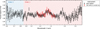 |
Fig. A.1 Comparison between the JWST NIRISS transmission spectrum from the standard reduction and the HST WFC3 spectrum from the CASCADe reduction (Crouzet et al. 2025). A small offset of 0.025 % was added to the HST WFC3 spectrum to allow for a better comparison of the spectral shapes. |
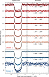 |
Fig. A.2 Representative spectral light curves of the NIRISS SOSS data with best-fit models (left) and residuals (right), spanning both spectral orders. Wavelength ranges (in μm) are annotated, and integer-percent offsets were applied to separate the bins. |
Appendix B Reduction tweaks
Figure B.1 provides a schematic overview of all the applied tweaks which are described in the following section. It also lists quantities derived from the differences in the resulting transmission spectra, that were calculated to quantify the impact on the spectrum. They are discussed in detail in the second subsection.
B.1 Description of tweaks
The only tweaks that were applied in the first two stages of the light curve extraction were related to the combined sky background and 1/ f noise removal. First, the effect of applying the 1/f noise correction to only the first or the second stage was tested. Second, three alternative methods for estimating the sky background were explored. The first two of these used alternative methods for determining scaling factors for the model background from the median stack of the out-of-transit images. One method, which is directly implemented in ExoTEDRF, applies a differential scaling by introducing a second region to account for areas of the detector affected by dispersed zodiacal light. The default region was used (x2 ∈ [715, 749], y2 ∈ [235,249]; see Fig. B.2). The other method applies a continuous scaling to each detector column. The custom scaling factors were derived by averaging the flux in a broader region of low target flux located above the third spectral order, followed by fitting a second-order polynomial to the column-averaged values. Specifically, all pixels located 40 pixels above the spectral trace were used, restricting the fit to columns with x < 1000 px. Columns with x < 230 px were explicitly excluded due to contamination from the fourth spectral order (Baines et al. 2024). In addition, a region with a width of 30 pixels around the step feature was also excluded from the fit. The third method derives a background estimate based solely on the median stack of the HAT-P-12b NIRISS observations. This was done by applying iterative sigma clipping (σ = 4) to identify the pixels least affected by target flux, which were subsequently again column-averaged. Regions identified by the procedure as nonbackground have been highlighted in Fig. B.2. This method mirrors the approach used in the CASCADe reductions of the NIRSpec and MIRI data (Crouzet et al. 2025; Bouwman et al., in prep.). Third, the remaining three 1/ f noise estimation methods implemented in ExoTEDRF were tested. The first, scale-achromatic-window, modifies the standard reduction method by restricting the pixels considered for the 1/f noise estimation to those within a specific radial range around the spectral traces. The second method scale-chromatic modifies the previous approach by using the first pass estimate of the spectral instead of the white light curves. The second, scale-chromatic, follows the same approach but uses the first pass spectral light curve instead of the white light curve. The third, solve, determines the scaling of the median stack without prior assumptions by simultaneously solving for both the scaling factor and the 1 / f noise amplitude. Further details are provided in the pipeline documentation7.
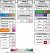 |
Fig. B.1 Schematic overview of the impact of the tested tweaked data reductions on the resulting transmission spectrum. Two metrics computed from the transit-depth differences relative to the standard reduction (∆δ) are reported: the weighted median μ1/2 and the Spearman rank correlation coefficient ρ, both listed and color-coded following the accompanying color bar. Tweaks are grouped by pipeline stage and ordered by execution, with the chosen method given on the left; the standard reduction choice is highlighted in bold, and select tweaked transmission spectra with large differences in trend are color-coded to match Fig. B.4). |
As noted earlier, no F277W exposure was obtained, preventing a direct measurement of contaminants isolated from the target flux. To still assess the impact of potential background sources, the data were visually inspected for signatures of contamination. No dispersed light from nontarget sources was identified. Several undispersed zeroth-order background sources are present, and two potential such contaminants are found to overlap with the cores of the target’s first and second spectral orders (see Fig. B.2). A custom interpolation method was employed to reconstruct the affected regions, using Gaussian-weighted averages of neighboring pixels on either side of each contaminant over a range of Δx = 20, px along the dispersion axis and within ry ± 20, px around the trace centroid along the spatial axis. The interpolated values were linearly blended across the contaminated columns. An additional tweak applied in the first part of the reduction involved the use of the alternative ATOCA extraction algorithm, which models crosscontamination between spectral orders (Darveau-Bernier et al. 2022).
For the light curve fitting, a number of tweaks affecting the light curve shape, but not directly originating from the planet, were tested. First, the impact of the adopted treatment of the LDCs was assessed by either fixing them to model values already at the white light curve level (fixed+fixed) or allowing them to vary freely within the Kipping (2013) parametrization also at the spectral light curve level (free+free). The differences between fitted and model-based LDC values are shown in Fig. B.3 for both the white and spectral light curves. In both cases, clear and systematic offsets are present. For the white light curves, the fitted values favor higher u1 and lower u2 compared to the model values for both spectral orders: order 1 (Δu1 = +0.14 = +9.36σ, Δu2 = −0.29 = −9.51σ) and order 2 (Δu1 = +0.11 = +6.21σ, Δu2 = −0.26 = −8.13σ). A similar behavior is observed for the spectral light curves (Δu1 =  =
=  , ∆u2 =
  =
=  ), where the relative trends between fitted and model values closely resemble those seen in the white light curves, differing primarily by an overall offset. Second, alternative nonflat baseline models of varying complexity were tested, namely a simple slope, a parabola, and the dominant ExoTEDRF-determined principal component analysis (PCA) component as a regressor. The parameters of the baseline models were allowed to vary freely and independently in their respective spectral light curve fits. Third, the impact of stellar contamination from spot crossing events was assessed by coupling the spotrod (Béky et al. 2014) code with the juliet framework, following an approach similar to the one presented in Fournier-Tondreau et al. (2024, 2025) including the construction of a single combined white light curve from both spectral orders. Scenarios with one and two spot crossing events were tested. For the spectral light curves, all parameters, except for the spot contrast f, were fixed to the values obtained from the white light curve fit.
The configuration files, scripts, and notebooks used to perform the tweaked reductions, as well as the resulting transmission spectra, are publicly available (see Data availability).
B.2 Impact on transmission spectrum
Given the number of tested tweaks and to allow for a clear and efficient comparison, the differences in the transmission spectrum caused by any particular tweak were summarized using two statistical metrics. First, the differences between the transit depths at all wavelengths ∆δ were calculated. From these differences, a weighted median μ1/2 using the inverse of the combined uncertainties as weights was calculated to quantify any general offset. Additionally, Spearman’s rank correlation coefficient ρ was computed to assess differences in the overall trend. The resulting values are listed in the diagram in Fig. B.1.
Only a few tweaks lead to offsets μ1/2 > 100 ppm (approx. mean uncertainty of standard reduction), or yield a Spearman coefficient |p| ≳ 0.2, indicating a strong wavelength-dependent trend. Four exemplary reductions with particularly high correlation coefficients (highlighted in Fig. B.1) are shown in Fig. B.4. Given that the retrievals freely fit for an offset between the different instruments, a pure shift in the spectral baseline is not expected to influence the retrieval results. Therefore, the differences were centered by subtracting the previously calculated weighted median values. There is a general trend of increased discrepancies (≳ 200 ppm) at both of the noisier ends of the spectrum, with the shortest wavelengths of the second order being affected more strongly. Except for two tweaked reductions that exhibit generally higher localized scatter, the centered differences remain within the 1σ uncertainty limits of the standard reduction. Applying the 1/f noise correction only in the second stage results not only in a large overall offset (~ 100 ppm), but also in localized differences across the entire wavelength range, with particularly pronounced deviations at its extremes (up to ~400ppm). In contrast, no such large discrepancies are observed when the 1/f noise correction is only applied in the first stage. This highlights the importance of performing the 1/f noise correction already at the group level, rather than postponing this correction to the integration level where the noise from multiple groups has been combined. For the background estimation, the sigma clipping method most strongly affects the overall shape of the transmission spectrum; notable differences of ρ = −0.4 also arise when using the custom scaling of the model background. Both result in a steeper slope at the short-wavelength end. This region is particularly sensitive due to two complementary factors: Firstly, the second spectral order reaches its short-wavelength limit in the strongly illuminated right part of the detector (cf. Fig. B.2). Secondly, the flux of the second order is decreasing toward shorter wavelengths leading to an increasing dominance of the flux from the first order despite increasing trace separation (maximum in flux ratio and ATOCA estimate of cross-contamination). Neither tweak introduces a significant global offset. The alternative treatments of the LDCs by keeping them free or fixed for the white and spectral light curves both have significant impacts on offset (|μ1/2| ≥ 125ppm) and trend (|p| ≥ 0.3). This is consistent with the well-established finding that strong degeneracies between LDCs and orbital parameters, such as the impact parameter b, can introduce significant biases (Espinoza & Jordán 2015; Alexoudi et al. 2020). These can also simply arise from the chosen parametrization itself and can cause significant wavelength-dependent biases across JWST modes, including NIRISS SOSS (Coulombe et al. 2024).
The choice of the baseline model does not introduce significant trends or offsets. Fitting for a linear slope (Δ ln Z = −2.05 ± 0.18), a quadratic parabola (Δ ln Z = −4.36 ± 0.18), or the dominant PCA component determined by the ExoTEDRF pipeline (Δ ln Z = −11.97 ± 0.17) all result in lower Bayesian evidence, indicating a clear preference for the simpler flat baseline model. In contrast, spot modeling reveals a strong preference for the inclusion of a single spot (Δ ln Z = +8.85 ± 0.14), while modeling two spots is disfavored (Δ ln Z = −1.73 ± 0.14). While there is a larger offset in the two spot case (|μ1/2| = 165 ppm) it remains very moderate in the single spot case (|μ1/2| = 21 ppm). The difference in the shape of the resulting transmission spectra, however, remains small in both cases (|p| ≤ 0.1). Retrievals using all JWST data but replacing the NIRISS spectrum with that from the tweaked reductions yield negligible changes for most detected molecules (< 0.07 dex, ≲0.11σ) except for H2S (≲0.2 dex, ≲0.5σ), and only slightly larger yet still minor differences (≲0.3 dex, < 0.08σ) for non-detected molecules.
 |
Fig. B.2 Overview of the data recorded by the NIRISS detector, based on a stack of out-of-transit integration images. The spectral orders are labeled; a different color scale is applied to enhance the visibility of the faint fourth order (gray rectangle). Regions used for scaling the model background and the location of the background step are highlighted (red and green). Areas identified via sigma clipping as containing signal (rather than background) are masked (white). The locations of two potential zeroth-order contaminants overlapping with the spectral traces are also indicated. For better visibility, these regions are shown with a separate color scale and an enlarged box (2 × ∆x) compared to the area that was interpolated over. |
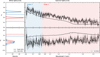 |
Fig. B.3 Comparison of the quadratic limb darkening coefficients (LDCs) u1 and u2 obtained when fitting them as free parameters (dashed lines) or fixing them (solid lines) to values calculated with the ExoTiC-LD package (Grant & Wakeford 2024) using the Stagger model grid (Magic et al. 2015), shown for both the white and spectral light curves. Color is used to distinguish between the first (red) and second (blue) spectral orders. For the white light curves, the full marginal posterior distributions of the LDCs are shown, while for the spectral light curves the median values (lines) and 1σ limits (gray shading) are displayed. In cases with free LDCs, the Kipping (2013) parametrization (q1, q2) was used, with samples transformed to u 1 and u2 for visualization. The free LDCs for the spectral light curves were obtained using the orbital parameters from the white light curve fit in which the LDCs were also fitted freely (free+free). |
 |
Fig. B.4 Impact of select reduction tweaks, shown as differences between the tweaked and standard-reduction transmission spectra. The differences were calculated by subtracting the weighted median μ1/2 from the transit depth differences ∆δ. This centering removes global offsets and emphasizes wavelength-dependent trends. For comparison, the 1σ uncertainty range of the standard reduction is indicated via dashed lines. |
Appendix C Retrievals
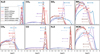 |
Fig. C.1 Same as Fig. 4, but instead of all JWST combinations only those that include NIRISS SOSS are shown and compared to the results obtained when HST WFC3 is used instead. |
Retrieved molecular abundances for all possible combinations of JWST instruments.
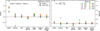 |
Fig. C.2 Differences in the retrieved chemical abundances between the standard N-point profile (XNP) and a simpler isothermal profile (Xiso). In the left panel, the differences are shown as absolute differences in the logarithmic VMRs ∆ log X, whereas in the right panel, the differences are scaled by the combined uncertainty σ calculated by adding the individual 1σ interval widths of the VMRs in quadrature. For the cases of significant detections the median abundance is used for the comparison, while for non-detections the upper 95th percentile serves as the reference point. |
C.1 Impact of offset treatment
 |
Fig. C.3 Same as Fig. C.2, but showing the abundance differences between retrievals with instrumental offsets included as free parameters in the nested sampling (XNS) and those optimized separately via least-squares (XLS). All instrument combinations considered in this work, except those including HST STIS data, are shown. |
While all multi-instrument retrievals conducted in this study include instrumental offsets between datasets, two different treatments were adopted. For all retrievals except those involving HST STIS data, the offsets Δδ0,z were included as free parameters in the nested sampling. For retrievals involving STIS data, the offsets were instead determined via a separate leastsquares optimization outside the nested sampling, following the approach also used for other ARCiS retrievals in earlier work in this series (Crouzet et al. 2025). Including the offsets directly in the nested sampling is, in principle, the more consistent approach, as it accounts for potential degeneracies with atmospheric parameters such as molecular abundances and cloud opacity parameters. Additionally, optimizing the offsets outside the nested sampling can bias the Bayesian evidence estimates, and thus the inferred detection significances, since it introduces parameters that are not explored within the sampling. However, this treatment comes with a significant computational overhead. While the increase in the number of model evaluations is typically modest (up to a factor of −2) for two-instrument combinations, it can reach a factor of −4 for three-instrument combinations (e.g., NIRISS+NIRSpec+MIRI: from ~4.2 × 10⁶ to ~1.8 × 10⁷ model evaluations). This substantial computational overhead is the reason why the alternative least-squares offset treatment was adopted for the retrievals including the HST STIS data. These retrievals involve the highest number of independent datasets (four in total) and are therefore expected to incur the largest increase in total runtime due to the chosen offset treatment. Combined with the increased per-model evaluation time due to the higher number of data points, this renders these retrievals computationally unfeasible within the scope of this work.
To compensate for this limitation, retrievals using the leastsquares optimization were also performed for all other instrument combinations, enabling an assessment of the impact of the offset treatment on the retrieved parameters and Bayesian evidence. Differences in the retrieved parameters and detection significances remain generally minor, with the only notable exceptions being the NIRISS+MIRI combination, and to a much lesser extent WFC3+MIRI. These are the only instrument combinations with a significant wavelength gap (>1.9 μm), compared to the otherwise near-continuous coverage (<0.03 μm), with the exception of the gap between WFC3 and NIRSpec at −1.2 μm. The least-squares treatment yields spurious tentative evidence for CO in the NIRISS+MIRI combination (2.6σ), and a weak preference of similar significance for the N-point over the isothermal T-P profile. As shown in Fig. C.3, this is also the only combination for which differences in the marginal chemical abundances between the two methods exceed 0.3 dex, with WFC3+MIRI showing the next largest deviations, exceeding those of all remaining combinations by more than 0.1 dex. Scaled by the uncertainties of the marginal abundances, however, the differences remain small, below 0.2σ in all cases, with the sole notable outlier being H2O for the NIRISS+MIRI combination at −0.9σ. While this demonstrates that the choice of offset treatment can introduce systematic differences, supporting the inclusion of instrumental offsets in the nested sampling, the results also show that these differences remain minor in the absence of wide wavelength gaps. Given the lack of such gaps in the retrievals involving the STIS data and the negligible impact of the low-resolution optical HST STIS data on molecular abundances, both in practice and as expected from molecular opacities, this justifies the adopted trade-off between computational cost and statistical rigor.
All Tables
Parameters used for the standard reduction and retrievals, with priors and posteriors from the white light curve fit.
Retrieved molecular abundances for all possible combinations of JWST instruments.
All Figures
|
Fig. 1 White light curves created from the first two spectral orders of the NIRISS SOSS data and combined best-fit model. The top panels show the observed data and fitted model light curves, while the bottom panels show the standardized residuals. The standardized residuals are the residuals divided by the uncertainty σφ that combines the uncertainties in flux reported by the pipeline σt with the additional jitter term σω fitted by the juliet framework ( |
| In the text | |
|
Fig. 2 Visualization of the HAT-P-12b transmission spectrum and the underlying opacity contributions. The top panel shows combined spectra from the three JWST instruments and HST STIS (Alexoudi et al. 2020) with 1σ uncertainties, together with the best-fit model with its 3σ credible interval. Model spectra including only the opacity of individual contributors (chemical species or cloud parametrization) are also shown. The bottom panel shows absorption cross sections (σ) of all tested chemical species. Significantly detected species are emphasized with thicker lines. |
| In the text | |
|
Fig. 3 Venn diagrams of JWST instrument combinations showing detection significances of the four significantly detected molecules (top) and the preference for two modeling assumptions (bottom). Additional circles show the significances obtained when replacing the JWST NIRISS SOSS with the HST WFC3 instrument data. The significances are reported as log-evidence differences ∆ ln Z and visualized using a custom nonlinear color scale. The color bar also provides a conversion to nσ detection significances following the calibration scale from Benneke & Seager (2013). |
| In the text | |
|
Fig. 4 Marginal posterior distributions of the chemical abundances for all included molecules, retrieved using different JWST instrument combinations. The shown distributions were derived from the samples via kernel density estimation (Gaussian kernel with bandwidth h = 0.1). For each distribution, the markers indicate either the 1σ credible interval for well-constrained posteriors or the 95th percentile upper limit (arrows) when only an upper bound can be established. |
| In the text | |
|
Fig. 5 On the left, an excerpt of the corner plot focusing on parameters of the cloud parametrization is shown. The joint posterior distributions (off-diagonal panels) are only shown for the retrieval using all JWST instruments and are visualized using contour lines smoothed with a Gaussian kernel (σ = 1). The marginal posterior distributions (diagonal panels) are additionally shown for exemplary JWST instrument combinations, as well as the results from retrievals that include the two HST STIS reductions. The same kernel density estimation as in Fig. 4 was applied. Additionally, in the upper right, a comparison of T-P profiles derived for the more complex N-point and the simpler isothermal parametrizations for the case of the three JWST instrument combination is shown. The lines indicate the median value, while the shaded regions are used to highlight the [0.5, 1,2,3] σ credible intervals. |
| In the text | |
|
Fig. 6 Marginal posterior distributions of the C/O ratio and metallicity ([(C+O)/H]) derived from molecular abundances for all JWST instrument combinations. An additional retrieval of all JWST instruments using the NIRSpec TEATRO instead of the standard CASCADe reduction is also shown (labeled TEATRO). The interval markers follow the convention introduced in Fig. 4. Solar (⊙; Asplund et al. 2021) and stellar (★; Biazzo et al. 2022) values are indicated on the top axis. The gray shading marks the uncertainty in the stellar values. |
| In the text | |
|
Fig. A.1 Comparison between the JWST NIRISS transmission spectrum from the standard reduction and the HST WFC3 spectrum from the CASCADe reduction (Crouzet et al. 2025). A small offset of 0.025 % was added to the HST WFC3 spectrum to allow for a better comparison of the spectral shapes. |
| In the text | |
|
Fig. A.2 Representative spectral light curves of the NIRISS SOSS data with best-fit models (left) and residuals (right), spanning both spectral orders. Wavelength ranges (in μm) are annotated, and integer-percent offsets were applied to separate the bins. |
| In the text | |
|
Fig. B.1 Schematic overview of the impact of the tested tweaked data reductions on the resulting transmission spectrum. Two metrics computed from the transit-depth differences relative to the standard reduction (∆δ) are reported: the weighted median μ1/2 and the Spearman rank correlation coefficient ρ, both listed and color-coded following the accompanying color bar. Tweaks are grouped by pipeline stage and ordered by execution, with the chosen method given on the left; the standard reduction choice is highlighted in bold, and select tweaked transmission spectra with large differences in trend are color-coded to match Fig. B.4). |
| In the text | |
|
Fig. B.2 Overview of the data recorded by the NIRISS detector, based on a stack of out-of-transit integration images. The spectral orders are labeled; a different color scale is applied to enhance the visibility of the faint fourth order (gray rectangle). Regions used for scaling the model background and the location of the background step are highlighted (red and green). Areas identified via sigma clipping as containing signal (rather than background) are masked (white). The locations of two potential zeroth-order contaminants overlapping with the spectral traces are also indicated. For better visibility, these regions are shown with a separate color scale and an enlarged box (2 × ∆x) compared to the area that was interpolated over. |
| In the text | |
|
Fig. B.3 Comparison of the quadratic limb darkening coefficients (LDCs) u1 and u2 obtained when fitting them as free parameters (dashed lines) or fixing them (solid lines) to values calculated with the ExoTiC-LD package (Grant & Wakeford 2024) using the Stagger model grid (Magic et al. 2015), shown for both the white and spectral light curves. Color is used to distinguish between the first (red) and second (blue) spectral orders. For the white light curves, the full marginal posterior distributions of the LDCs are shown, while for the spectral light curves the median values (lines) and 1σ limits (gray shading) are displayed. In cases with free LDCs, the Kipping (2013) parametrization (q1, q2) was used, with samples transformed to u 1 and u2 for visualization. The free LDCs for the spectral light curves were obtained using the orbital parameters from the white light curve fit in which the LDCs were also fitted freely (free+free). |
| In the text | |
|
Fig. B.4 Impact of select reduction tweaks, shown as differences between the tweaked and standard-reduction transmission spectra. The differences were calculated by subtracting the weighted median μ1/2 from the transit depth differences ∆δ. This centering removes global offsets and emphasizes wavelength-dependent trends. For comparison, the 1σ uncertainty range of the standard reduction is indicated via dashed lines. |
| In the text | |
|
Fig. C.1 Same as Fig. 4, but instead of all JWST combinations only those that include NIRISS SOSS are shown and compared to the results obtained when HST WFC3 is used instead. |
| In the text | |
|
Fig. C.2 Differences in the retrieved chemical abundances between the standard N-point profile (XNP) and a simpler isothermal profile (Xiso). In the left panel, the differences are shown as absolute differences in the logarithmic VMRs ∆ log X, whereas in the right panel, the differences are scaled by the combined uncertainty σ calculated by adding the individual 1σ interval widths of the VMRs in quadrature. For the cases of significant detections the median abundance is used for the comparison, while for non-detections the upper 95th percentile serves as the reference point. |
| In the text | |
|
Fig. C.3 Same as Fig. C.2, but showing the abundance differences between retrievals with instrumental offsets included as free parameters in the nested sampling (XNS) and those optimized separately via least-squares (XLS). All instrument combinations considered in this work, except those including HST STIS data, are shown. |
| In the text | |
Current usage metrics show cumulative count of Article Views (full-text article views including HTML views, PDF and ePub downloads, according to the available data) and Abstracts Views on Vision4Press platform.
Data correspond to usage on the plateform after 2015. The current usage metrics is available 48-96 hours after online publication and is updated daily on week days.
Initial download of the metrics may take a while.