| Issue |
A&A
Volume 699, July 2025
|
|
|---|---|---|
| Article Number | A250 | |
| Number of page(s) | 12 | |
| Section | Stellar structure and evolution | |
| DOI | https://doi.org/10.1051/0004-6361/202555151 | |
| Published online | 10 July 2025 | |
Shaping core dynamos in A-type stars: The role of dipolar fossil fields
1
Dipartimento di Fisica, Sapienza, Università di Roma, Piazza le Aldo Moro 5, 00185 Roma, Italy
2
Institut für Sonnenphysik (KIS), Georges-Köhler-Allee 401a, 79110 Freiburg, Germany
3
Hamburger Sternwarte, Universität Hamburg, Gojenbergsweg 112, 21029 Hamburg, Germany
4
Institute of Space Sciences (ICE-CSIC), Campus UAB, Carrer de Can Magrans s/n, 08193 Barcelona, Spain
⋆ Corresponding author.
Received:
14
April
2025
Accepted:
30
May
2025
Context. Large-scale magnetic fields of Ap/Bp stars are stable over long timescales and typically have simple dipolar geometries, leading to the idea of a fossil origin. These stars are also expected to have convective cores that can host strong dynamo action.
Aims. Our aim was to study the interaction between the magnetic fields generated by the convective core dynamo of the star, and a dipolar fossil field reminiscent of observed magnetic topologies of Ap/Bp stars.
Methods. We used numerical 3D star-in-a-box simulations of a 2.2 M⊙ A-type star, where the core encompasses 20% of the stellar radius. As an initial condition, we imposed two purely poloidal configurations, both with a surface dipolar strength of 6 kG, and we explored different obliquity angles β (the angle between the magnetic and rotational axes), ranging from 0° to 90°.
Results. The inclusion of a poloidal field where none of the magnetic field lines are closed inside the star, does not affect the core dynamo in a significant way. Dipolar configurations where all the field lines are closed inside the star can enhance the dynamo, producing a superequipartition quasi-stationary solution, where the magnetic energy is five times stronger than the kinetic energy. The enhanced core dynamos have typical magnetic field strengths between 105 and 172 kG, where the strength has an inverse relation with β. The strong magnetic fields produce an almost rigid rotation in the radiative envelope, and change the differential rotation of the core from solar-like to anti-solar. The only cases where the imposed dipoles are unstable and decay are those with β = 90°. In the rest of the cases, the core dynamos are enhanced and the surface magnetic field survives, keeping simple topologies as in the observations.
Key words: dynamo / magnetohydrodynamics (MHD) / stars: early-type / stars: magnetic field
© The Authors 2025
 Open Access article, published by EDP Sciences, under the terms of the Creative Commons Attribution License (https://creativecommons.org/licenses/by/4.0), which permits unrestricted use, distribution, and reproduction in any medium, provided the original work is properly cited.
This article is published in open access under the Subscribe to Open model. Subscribe to A&A to support open access publication.
1. Introduction
Large-scale magnetic fields have been observed in around 10% of main-sequence (MS) early-type stars (Moss 2001; Kochukhov & Bagnulo 2006; Landstreet et al. 2007, 2008; Grunhut et al. 2017; Shultz et al. 2019). Unlike late-type stars, whose magnetic fields have complex geometries and evolve on relatively short timescales (see e.g., Suárez Mascareño et al. 2016), the observed magnetic fields of early-type stars have simpler geometries, and they are stable over long timescales, with virtually no variability over several decades (Donati & Landstreet 2009; Briquet 2015). The observed magnetic fields from late-type stars are very likely due to dynamo processes operating in their convective envelopes (see e.g., Charbonneau 2020, for the solar dynamo). Numerical simulations capture many elements of these dynamos (see e.g., Käpylä et al. 2023, and references therein). However, early-type stars have radiative envelopes, or very thin convective layers close to the surface due to peaks in the opacities (e.g., Richard et al. 2001; Cantiello et al. 2009). These thin layers are thought to produce surface magnetic fields on the order of a few gauss (Cantiello & Braithwaite 2019), but this is not sufficient to explain the observed large-scale magnetic fields of these stars. For example, chemically peculiar Ap/Bp stars, which are intermediate mass (1.5 − 6 M⊙) MS stars, host surface magnetic fields with mean strengths between 200 G and 30 kG (Shorlin et al. 2002; Aurière et al. 2007). In most cases the magnetic field is a simple dipole with its axis misaligned with the rotation axis (Donati & Landstreet 2009; Kochukhov et al. 2015). Some Ap/Bp stars exhibit more complex geometries, and multipoles are required to fit the data (e.g., Kochukhov & Wade 2016; Silvester et al. 2017). However, these multipolar fields seem to decay faster than the commonly observed dipolar fields (Shultz et al. 2019). As the origin of these large-scale magnetic fields cannot be explained via convective envelope dynamo, several theories have been proposed, such as a dynamo operating on the radiative layers as a result of the interaction of a magnetic instability and differential rotation. An example is the Tayler-Spruit dynamo scenario (Spruit 2002; Petitdemange et al. 2023, 2024).
However, the simple topologies and the stability over long timescales of the observed magnetic fields seem to support the idea of fossil fields, i.e., magnetic fields originating from an earlier stage of stellar evolution (Alecian et al. 2019). In the pre-MS evolution, Herbig Ae/Be stars (Waters & Waelkens 1998; Waters 2006) are believed to be the predecessors of MS Ap/Bp stars, and although their average magnetic fields are substantially weaker than those from Ap/Bp stars (see e.g., Hubrig et al. 2004; Kholtygin et al. 2019; Hubrig et al. 2020), they still share some common characteristics, such as their incidence rate (Hubrig et al. 2011; Alecian et al. 2013a,b). This suggests that the magnetic field is already present in the pre-MS stage, evolving from the molecular cloud to the MS (Moss 2003; Schleicher et al. 2023). It has also been proposed that the strong observed magnetic field could be the result of a merger with another protostar close to the end of the formation process (e.g., Ferrario et al. 2009; Schneider et al. 2019). In any case, the thick radiative envelope of Ap/Bp stars might provide the ideal conditions for the fossil magnetic field to reach a stable equilibrium and evolve on a diffusive timescale. Cowling (1945) realized that, in the radiative core of the Sun, this timescale is on the order of 1010 years; therefore, a magnetic field in equilibrium could survive for the entire MS lifetime of the star. However, finding stable configurations with analytical methods has been proven to be a challenging task. The energy method of Bernstein et al. (1958) shows that purely poloidal and purely toroidal fields in highly ideal conditions are unstable under perturbations (Tayler 1973; Markey & Tayler 1973; Wright 1973; Markey & Tayler 1974). Numerical MHD simulations by Braithwaite & Nordlund (2006) produced stable configurations in the radiative interior of a 2 M⊙ A-type star starting from an initially random field, which relaxed to a stable roughly axisymmetric torus inside the star, with poloidal and toroidal components of comparable strength, leading to a roughly dipolar surface field. Non-axisymmetric configurations have also been found, starting from turbulent initial conditions (Braithwaite 2008). Recently, simulations by Becerra et al. (2022) showed that random magnetic field configurations seem to always evolve to a stable equilibrium in stably stratified environments, thus confirming previous results.
In addition to deep radiative envelopes, early-type stars have convective cores due to the temperature sensitivity of the CNO cycle. These cores have vigorous convective motions and differential rotation that can lead to dynamo action (Browning et al. 2004). Strong core dynamos have been found in numerical 3D simulations (Brun et al. 2005; Augustson et al. 2016; Hidalgo et al. 2024). Recently, an upper limit of Br ≈ 500 kG was estimated for the B star HD 43317 by Lecoanet et al. (2022), based on its g-mode frequencies (Buysschaert et al. 2018). This limit seems to support the idea of a strong core dynamo inside these stars, due to the fact that this magnetic field strength would be hard to achieve exclusively with fossil fields. However, these magnetic fields are most likely unable to create large-scale structures on the stellar surface (Schuessler & Paehler 1978; Parker 1979; MacDonald & Mullan 2004), and only a very small percentage of the magnetic flux can be transported there (MacGregor & Cassinelli 2003; Hidalgo et al. 2024). Interestingly, a core dynamo can potentially interact with a fossil field (see Boyer & Levy 1984, in the context of the Sun). Featherstone et al. (2009) performed numerical simulations of a 2 M⊙ A-type star core dynamo initially hosting near-equipartition fields surrounded by a fraction of the radiative envelope. The inclusion of a fossil field with poloidal and toroidal components led to a superequipartition state where magnetic energy is roughly ten times stronger than kinetic energy. This might have some interesting implications; for example, if this magnetic field is strong enough, then a larger magnetic flux can possibly be transported to the surface by magnetic buoyancy (e.g., MacDonald & Mullan 2004). Furthermore, how an enhanced core dynamo affects the fossil field at the stellar surface and inside the radiative envelope is unknown.
Simulations studying the stability of magnetic fields assume a stably stratified environment and neglect the presence of a core dynamo (e.g., Braithwaite & Spruit 2004; Becerra et al. 2022). For the current study, we imposed a fossil field into a star-in-a-box setup of a MS A-type star hosting a core dynamo presented in Hidalgo et al. (2024) (hereafter Paper I). This setup allowed us to study how different fossil fields affect the core dynamo and how the surface magnetic field is modified. Another issue to be explored, is how the inclination of the fossil field affects the results, as in most of the Ap stars the axes of the magnetic dipole and rotation do not coincide. The models and methods are explained in Sect. 2. The initial state of the core dynamo and the explored fossil fields configurations are described in Sect. 3. The results of the simulations are discussed in Sect. 4. A summary of the study and our conclusions are presented in Sect. 5.
2. Numerical models
2.1. A-type star setup
The setup used here is the same as that in Paper I, which is based on the star-in-a-box setup from Käpylä (2021). The star has a radius R and it is embedded into a cube of side l = 2.2R, where the Cartesian coordinates range from −l/2 to l/2. The convective core encompasses 20% of the radial extent of the star, while the rest is stably stratified (see Paper I, for more details). The fully compressible set of MHD equations is:

![$$ \begin{aligned} T \frac{Ds}{Dt}&= - \frac{1}{\rho } \left[ \boldsymbol{\nabla } \boldsymbol{\cdot } (\boldsymbol{F}_\text{ rad} + \boldsymbol{F}_\text{ SGS}) + \mathcal{H} - \mathcal{C} + \mu _0 \eta \boldsymbol{J}^2 \right] + 2 \nu \boldsymbol{\mathsf{S}}^2, \end{aligned} $$](/articles/aa/full_html/2025/07/aa55151-25/aa55151-25-eq4.gif)
where A is the magnetic vector potential, U is the flow velocity, B = ∇ × A is the magnetic field, η is the magnetic diffusivity, μ0 is the magnetic permeability of vacuum, J = ∇ × B/μ0 is the current density,  is the advective derivative, ρ is the mass density, p is the pressure, Φ is the fixed gravitational potential obtained from a 1D model, ν is the kinematic viscosity, and
  is the traceless rate-of-strain tensor
where δij is the Kronecker delta. The rotation vector is  and
and  damps the flows outside the star, with
where τdamp = 0.2τff ≈ 1.5 days is the damping timescale,  is the freefall time, and

where  , rdamp = 1.03R is the radius where the damping starts, and where wdamp = 0.02R is its width. T is the temperature, s is the specific entropy, and Frad is the radiative flux

where K is the heat conductivity, and FSGS is the sub-grid-scale (SGS) entropy flux, which damps entropy fluctuations near the grid scale (see Käpylä 2021; Käpylä et al. 2023)
where χSGS is the SGS diffusion coefficient, s′=s − ⟨s⟩t is the fluctuating entropy, and  is a temporal mean of the specific entropy. Because the SGS diffusion applies to the fluctuations of the specific entropy, its contribution to net energy transport is negligible. The heating function ℋ follows
which is a normalized Gaussian that parameterizes the nuclear energy production in the core of the star, where Lsim is the luminosity in the simulation, and wL = 0.1R is the width of the Gaussian. The cooling function  is given by
which models radiative losses above the stellar surface, where cP is the heat capacity at constant pressure, Tsurf = T(R) is the temperature at the stellar surface, τcool = τdamp is a cooling timescale, and fe(r) is given by Eq. (7), with rcool = rdamp and wcool = wdamp. The ideal gas equation of state p = (cP − cV)ρT is assumed, where cV is the heat capacity at constant volume. The model has radial profiles for the diffusivities ν and η, where radiative zones have values that are 102 times smaller than in convective zones (Käpylä 2022). Furthermore, sixth-order hyperdiffusivity terms are added in the dynamical equations (see e.g., Brandenburg & Sarson 2002; Johansen & Klahr 2005; Lyra et al. 2017).
The simulations were run with the PENCIL CODE1 (Pencil Code Collaboration 2021), which is a highly modular high-order finite-difference code for solving ordinary and partial differential equations, on a grid of 2003 equally distributed grid points.
2.2. Units and relation to reality
The units of length, time, density, entropy, and magnetic field are given by
![$$ \begin{aligned}[x]=R, \ [t] = \tau _\mathrm{ff} , \ [\rho ] = \rho _0, \ [s] = c_{\rm P}, \ {[B]} = \sqrt{\mu _0 \rho _0}[x]/[t]. \end{aligned} $$](/articles/aa/full_html/2025/07/aa55151-25/aa55151-25-eq20.gif)
In this study, the quantities are typically expressed in physical units. The conversion factors are the same as those given by Eqs. (17) and (18) in Paper I. The stellar parameters where obtained from a 1D MESA model with 2.2 M⊙ (Paxton et al. 2019), and are the same as those from Paper I, i.e., the radius, mass density and temperature of the stellar center, and stellar luminosity are R⋆ = 2.1 R⊙, ρ0 = 5.5 ⋅ 104 kg m−3, T0 = 2.3 ⋅ 107 K, L⋆ = 23.5 L⊙, respectively. Furthermore, as we are using the fully compressible formulation of the MHD equations, the enhanced luminosity approach is also used in these simulations (see Dobler et al. 2006; Käpylä et al. 2020; Käpylä 2021, for a detailed justification). To have a consistent rotational influence on the flow, the rotation rate is enhanced following the recipe in Appendix A of Käpylä et al. (2020).
2.3. Diagnostics quantities
The rotational influence on the flow is measured by the global Coriolis number,

where urms is the root mean square (rms) velocity averaged over the convection zone and kR = 2π/Δr is an estimate of the largest convective eddies in the system, where Δr = 0.2R is the depth of the convective zone. The fluid and magnetic Reynolds numbers, and the SGS Péclet number are defined as
3. Imposing a magnetic field
3.1. Initial state of the simulation
To analyze how an imposed fossil field affects the core dynamo, the fossil field configurations are added to snapshots of an already saturated core dynamo simulation. We chose run MHDr2 from Paper I, which hosts a dynamo with the largest rotation period (Prot = 15 days) and therefore, the smallest Coriolis number (Co = 10.1) in that study. The core of this simulation (r < 0.2R) has a root-mean-square (rms) magnetic field of Brms = 60 kG, solar-like differential rotation, and a hemispherical dynamo with most of the activity located on its southern hemisphere. The snapshot where the fossil field was imposed corresponds to a simulated time of t = 4135τff, or 85 years in physical units. In Fig. 1(a,b) the radial and toroidal magnetic fields at the surface of the convective zone (r = 0.2R) from this snapshot are shown. Both magnetic field components are highly concentrated on the southern hemisphere. Furthermore, the amplitude of the toroidal component is larger than that of the radial component. Panel (c) displays the azimuthally averaged magnetic field in the entire box. The hemispheric nature of the core dynamo is still clearly visible from both components. However, strong magnetic fields are also present at the bottom radiative envelope. This is most likely due to flows penetrating into the radiative layer near the rotation axis. Finally, on panel (d) the azimuthally averaged flows are shown. The flows penetrating deeply into the radiative envelope are most likely due to lower Brunt-Väisälä frequency (for example, see Fig. 5 of Korre & Featherstone 2024), and therefore, lower Richardson numbers related to rotation than in real stars (e.g., Käpylä 2024) achieved in our simulations. These flows also transport some of the magnetic flux from the core dynamo to the stellar surface, leading to an rms surface magnetic field of ∼0.1 kG at the poles and as low as 10−5 kG elsewhere. MHDr2 has subequipartition magnetic fields, where the ratio of the magnetic to kinetic energies is Emag/Ekin = 0.196 in the convective core (r < Δr), and 0.322 in the entire star (r < R).
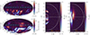 |
Fig. 1. Magnetic fields and flows from a snapshot of MHDr2 at t = 85 yr. Panels (a), (b): Radial and toroidal magnetic fields at the surface of the convective zone (r = 0.2R). Panel (c): Azimuthally averaged toroidal (colormap) and poloidal (arrows) magnetic fields. Panel (d): Azimuthally averaged toroidal flows (colormap) and meridional circulation (arrows). All the panels are clipped for a better display, and the minimum and maximum values are indicated below the colorbar. |
3.2. Dipolar fossil field
The majority of Ap stars exhibit large-scale poloidal magnetic fields. For example, in HD 75049, 90% of magnetic energy is concentrated in the dipolar ℓ = 1 spherical harmonic mode with a polar strength of Bp = 36 kG and an obliquity of 36° (Kochukhov et al. 2015). Similarly, in HD 24712, 96% of the magnetic energy is concentrated in ℓ = 1 (Rusomarov et al. 2015). Therefore, we choose to impose a purely poloidal (Bϕ = 0) fossil field, whose vector potential is
where m is the magnetic dipole moment. As discussed, the observed magnetic fields of Ap/Bp stars are typically misaligned with their rotation axis. Therefore, we define m as

where β is the obliquity angle of the magnetic dipole with respect to Ω, and m0 is the initial dipolar amplitude. Thus, Eq. (15) can be expressed as

The sample of Ap stars presented by Landstreet & Mathys (2000) shows that slow rotators (Prot > 25 days) have small obliquity angles, with an excess around 20°, while fast rotators tend to have larger values of β. More recently, Shultz et al. (2019) reported that the distribution of β seems to be statistically consistent with a random distribution, which fits with the data of Aurière et al. (2007), and Sikora et al. (2019, see their Fig. 11). In this study, we consider 0° ≤β ≤ 90°. More specifically, β = 0° (0), 30° (π/6), 60° (π/3) and 90° (π/2), to explore the entire range of inclinations. We further test β = 80° (4π/9) and 85° (17π/36) in one specific case, to study the transition to a horizontal dipole in more detail.
We define two dipolar initial conditions. The first (Dipole A) corresponds to the magnetic field of a magnetized sphere, i.e., a uniform magnetic field inside (r < R), matched by a dipole field in the exterior (r > R). The second configuration corresponds to a dipole field in the entire domain. Eq. (17) has a singularity for r → 0, and therefore we added a constant ϵ to r, such that r′≡r + ϵ is used in the calculation of the dipole fields. Two values of ϵ were chosen, where ϵ1 < ϵ2. ϵ1 (ϵ2) produces a Brmspol of roughly 500 kG (100 kG) in the core, r < 0.2R, and 48 kG (14 kG) in the entire star. The runs with ϵ1 are labeled as Dipole B* and those with ϵ2 as Dipole B. The initial value of m0 was chosen such that all the mentioned magnetic configurations have a dipolar amplitude of roughly 6 kG at the stellar surface, which is typical from Ap/Bp stars (Aurière et al. 2007; Shultz et al. 2019). All of the initial conditions are displayed in the first three panels of Fig. 2. An obliquity angle of 30° was added in Dipole B (third panel) as an example of a tilted dipole initial condition.
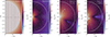 |
Fig. 2. Imposed initial (fossil) magnetic fields in our simulations. The arrows represent the poloidal magnetic field lines, and the colormap the intensity of this component. Dipole A and Dipole B* are aligned to the rotational axis (β = 0°), and as an example of a misaligned dipole an inclination of β = 30° was added in Dipole B. The last panel corresponds to the initial snapshot of run DipB (Dipole B + MHDr2). |
4. Results
The simulations are divided into three sets, the names of which reflect the chosen initial configuration. For example, runs with Dipole B are labeled as DipB. The simulations, as well as the diagnostic quantities, are listed in Table 1.
Summary of the simulations.
4.1. Core dynamos
All of the current simulations host a strong core dynamo. However, in some cases the dynamo is enhanced by the fossil field while in others it remains mostly unaffected (see Table 1). More specifically, runs with Dipole A have essentially the same Brms as the run with no added dipole (MHDr2), irrespective of the inclination angle (see upper panel of Fig. 3). On the other hand, runs with Dipoles B and B* have stronger core magnetic fields, in some cases thrice that of MHDr2. Interestingly, in the latter two sets there is a relation between the strength of the magnetic fields and the obliquity angle β.
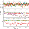 |
Fig. 3. Temporal evolution of the rms magnetic field in the convective core (r < 0.2R) from all simulations. The gray dashed line indicates 60 kG, which is the saturated value of the core dynamo from MHDr2. |
4.1.1. Enhanced dynamos
Figure 3 shows that runs with Dipoles B and B* start with the same core magnetic field amplitudes, and that only the cases with β = 90° decay to the same level as the core dynamo without any additional dipole field (the gray dashed line). The aligned cases (DipB, DipB*) and the rest of inclinations (DipBt, DipBt2, DipBt*, DipBt2*, DipBt3*, DipBt4*) saturate in higher values than those of run MHDr2, suggesting enhanced core dynamo action. The saturation levels of these runs are similar although temporal averages (fourth column of Table 1) show that there is an inverse relation between β and Brms. The strongest rms magnetic fields for both averages, are obtained when the dipole is aligned with the rotation axis. In the misaligned cases the field decreases with increasing β. The only exception to this trend is DipBt*, which has the same averaged flow velocity and rms magnetic fields as DipB*. Interestingly, inside the core, DipBt* has even a stronger toroidal component than DipB*, while in the rest of runs the inverse relation applies for both poloidal and toroidal components. Furthermore, weaker magnetic fields lead to weaker quenching of flows. It is worth mentioning that although we only added a strong poloidal component in the simulations, the toroidal component of the core dynamo also increases in the enhanced cases. The cases with horizontal dipoles decayed almost completely. These runs will be analyzed separately in Sect. 4.1.2.
The azimuthally averaged toroidal magnetic fields at r = 0.2R as a function of time and latitude for representative enhanced cases are shown in Fig. 4. The initially cyclic and hemispheric solutions (see Fig. 2 of Paper I) are replaced by quasi-stationary solutions. All the simulations with an enhanced core dynamo end up in the same configuration, irrespective of the obliquity angle. Quasi-stationary dynamosolutions appear in simulations either with low Coriolis numbers (e.g., Käpylä et al. 2013; Strugarek et al. 2018; Brun et al. 2022; Ortiz-Rodríguez et al. 2023), or in the strong field branch at rapid rotation (e.g., Christensen & Aubert 2006; Gastine et al. 2012; Yadav et al. 2015). The current simulations land in the latter due to the strong added dipole fields. The obtained configuration resembles a dipole, with a positive polarity in latitudes from 0° to 30° and negative polarity from 0° to −30°. Beyond these latitudes, the polarity reverses, and the magnetic fields are weaker than in the latitudes close to the equator. As the added dipole field is purely poloidal, the toroidal fields likely come from a dynamo process in the convective core.
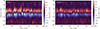 |
Fig. 4. Time-latitude diagrams of the azimuthally averaged toroidal magnetic field |
To understand the origin of these dynamos, we make use of dynamo numbers based on mean-field dynamo theory (Krause & Rädler 1980; Brandenburg & Subramanian 2005). To quantify the α and Ω effects, it is useful to define (Käpylä et al. 2013)
where ηturb = τurms2/3 is an estimate of the turbulent diffusivity, τ = Δr/urms is the convective turnover time, and  is the time- and azimuthally averaged rotation rate. The non-linear α effect is proportional to the difference between the fluctuating kinetic and magnetic helicities, given by (Pouquet et al. 1976)
![$$ \begin{aligned} \alpha = - \frac{\tau }{3}\left[(\overline{\boldsymbol{U} \boldsymbol{\cdot } \boldsymbol{\omega }} - \overline{\boldsymbol{U}} \boldsymbol{\cdot } \overline{\boldsymbol{\omega }})-(\overline{\boldsymbol{J} \boldsymbol{\cdot } \boldsymbol{B}} - \overline{\boldsymbol{J}} \boldsymbol{\cdot } \overline{\boldsymbol{B}})/\overline{\rho }\right], \end{aligned} $$](/articles/aa/full_html/2025/07/aa55151-25/aa55151-25-eq29.gif)
where ω = ∇ × U is the vorticity. The dynamo parameters (18) from DipB and MHDr2 are shown in Fig. 5. The profiles and amplitudes of cα in the current simulations are similar to those of runs without a fossil field (see left panels of Fig. 5). However, the enhanced cases show zones of strong α effect with a different sign close to the equator. These are also the locations where the magnetic field is the strongest (see Fig. 4). The profile of cα is antisymmetric with respect to the equator. The profiles of cΩ are of opposite sign in comparison to those of runs in Paper I. This is a consequence of the anti-solar differential rotation of the core (see Sect. 4.3). The amplitudes of cΩ are also much weaker than in Paper I. This is clearly seen in the right panels of Fig. 5. The inclusion of a strong imposed field quenches the differential rotation, reducing the shear, which is translated in lower values of cΩ. Table 2 shows that the energy in differential rotation in the core and in the radiative envelope is weaker than in MHDr2. Furthermore, in the enhanced dynamos, the poloidal energy is stronger than the toroidal energy, being typically Emagpol ≈ 3Emagtor.
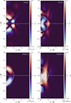 |
Fig. 5. Dynamo parameters cα = αΔr/ηturb and |

Kinetic and magnetic energies.
We interpreted the core dynamos from Paper I as αΩ or α2Ω dynamos, primarily because the signs of α,  and the propagation direction of the dynamo waves, and secondarily, because cΩ ≫ cα and the dominance of toroidal over poloidal fields. In the enhanced dynamos, the lower values of cΩ, weaker than cα in some runs, and the ratio Emagpol/Emagtor ≈ 3 suggest an α2 dynamo. These dynamos rely on the α effect, and no shear from differential rotation is directly needed. Their initial formulation suggested only non-oscillatory dynamos, for example, the axisymmetric models by Steenbeck & Krause (1969), which fits with the quasi-stationary solutions of the axisymmetric toroidal magnetic field found in our simulations. However, oscillatory solutions have also been found in numerical simulations (Baryshnikova & Shukurov 1987; Mitra et al. 2010; Käpylä et al. 2013; Masada & Sano 2014) and analytical work (Raedler & Braeuer 1987; Brandenburg 2017).
The meridional distribution of the azimuthally averaged magnetic field of DipB is shown in Fig. 6. In an early stage of the simulation, five years (∼240τff) after the inclusion of the fossil field, the core dynamo already exhibits the described quasi-stationary behavior (see left panel). Furthermore, some of the toroidal magnetic fields are seen outside the convective core, at the base of the radiative envelope. The poloidal magnetic field follows the structure of Dipole B outside the core, while within it, the field is nearly vertical, as it is in Dipole A. The magnetic field in the radiative zone is different than that generated by the core dynamo without an added dipole (see Fig. 4 of Paper I). Initially, the magnetic field spread close to the rotation axis from z ≈ 0.3R to r ≈ 0.5R, which is the location of the magnetic diffusivity jump. In Paper I we mention that this magnetic field is most likely transported by vertical flows (see, e.g., the rightmost panel of Fig. 1), after which it evolves on long timescales compared to the period of the core dynamo due to the low diffusivities there. In the current simulations, there is much less magnetic fields beyond the radial jump of diffusivities (r ≈ 0.35R), indicating that in runs with the enhanced core dynamo the flows are not transporting magnetic field from the core to this zone as efficiently. The right panel of Fig. 6 displays the magnetic field of DipB 82 years (or ∼3993τff) after that in left panel. The quasi-stationary nature of the core dynamo remains unaffected. Furthermore, the dipolar structure present in most of the radiative envelope and at the stellar surface remains essentially unchanged, indicating that the enhanced core dynamo influences the surface poloidal magnetic field of the star only weakly (see Sect. 4.2).
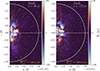 |
Fig. 6. Azimuthally averaged toroidal magnetic field |


Finally, these runs have superequipartition magnetic fields. More specifically, DipB* and DipBt* have Emag/Ekin ≈ 5 in the convective core, and Emag/Ekin ≈ 10 in the radiative envelope. The core dynamo of the fast rotators from Augustson et al. (2016) achieve similar regimes as those in our simulations, for example, their fastest rotator (M16) reaches Emag/Ekin = 5.02. While still in superequipartition, it is unclear how Emag/Ekin changes in the simulations of Featherstone et al. (2009) with an added purely poloidal field. Nevertheless, the inclusion of a mixed field (with poloidal and toroidal components) increases the ratio in the core dynamo to Emag/Ekin ≈ 10. This ratio is comparable to what we find in the radiative envelope of our runs but larger than in our core dynamos. In the mixed case of Featherstone et al. (2009), Emag/Ekin ≈ 5.18 in the radiative envelope (see their Table 1), which is less than in our simulations. This might be because they consider only a fraction of the radiative envelope. In runs with Dipole B, the enhanced dynamos are also in the superequipartition regime, but the ratios are somewhat smaller than those from runs with Dipole B*, both in the convective core and in the radiative zone.
4.1.2. The unaffected cases
The azimuthally averaged toroidal magnetic fields at r = 0.2R of representative simulations without an enhanced dynamo are shown in Fig. 7. None of the core dynamos from runs with Dipole A got enhanced, and the obliquity angle of the dipole has no effect in the magnetic field configuration. This is likely a consequence of the strength of the dipole. While all the configurations have a surface dipolar amplitude of 6 kG, Dipole A keeps this amplitude constant inside the star, and therefore, Brmspol inside the core is ∼6 kG. This is much weaker than the fields from Dipoles B and B* (see Sect. 3.2) or that from the core dynamo of MHDr2 (∼19 kG). Furthermore, their magnetic cycle period is not affected either, being essentially the same as that from MHDr2 (see the last column of Table 1). Figure 7 shows that the core dynamo from DipA remains cyclic and hemispheric, occasionally changing its active hemisphere, similar to run MHDr2* of Paper I and in the fully convective model of Brown et al. (2020). All the runs with Dipole A show at least one dynamo migration except DipAh. One difference between these runs and MHDr2 is that close to the equator a weak structure similar to the quasi-stationary solutions of the enhanced dynamos is visible, except in DipAh. For example, this structure can be spotted in DipA where it is clearest between ∼130 and ∼150 years.
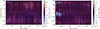 |
Fig. 7. Same as Figure 4, but for runs without an enhanced dynamo. |
The right panel of Figure 7 display the toroidal magnetic field of the horizontal case (β = 90°) with Dipole B*. In this case, the core dynamo exhibits the quasi-stationary solution described in Sect. 4.1.1 right after the inclusion of the dipole field. However, the solution is unstable and it decays after a few years, returning to the original hemispherical configuration of the core dynamo. The same happens in DipBh. Interestingly, this fast decay happens exclusively in the horizontal cases, whereas even the cases with β = 80° and β = 85° have a stable enhanced dynamo with at least twice the strength of the horizontal cases (see Table 1).
4.2. Stability and surface magnetic fields
In principle, a purely poloidal magnetic field whose field lines are closed inside the star, as in Dipole B and Dipole B*, is unstable against adiabatic perturbations (Markey & Tayler 1973; Wright 1973; Markey & Tayler 1974). Similarly, a poloidal field with none of the field lines closed inside the star, as in Dipole A, is unstable as well (Flowers & Ruderman 1977). However, these analytical results are highly idealized, as dissipative effects and rotation are not considered. Furthermore, we are not testing the stability of a purely poloidal magnetic field. In MHDr2, 37.8% of the magnetic energy inside the radiative envelope is toroidal, and as described in Sect. 4.1.1, the added poloidal field can also induce a toroidal component close to the core. Therefore, the radiative envelopes in our simulations have both components in all the cases, which as suggested by analytical estimations (Prendergast 1956; Wright 1973), and numerical results (Braithwaite & Spruit 2004; Braithwaite & Nordlund 2006), seems to be a necessary condition to achieve stability. Furthermore, the stability condition reported by Braithwaite (2009) suggests 10−5 ≲ Emagpol/Emag ≲ 0.8 for a MS A-type star, which is fulfilled inside the radiative envelope in all of our simulations (see column 7 of Table 2).
The upper panels of Figure 8 show the latitudinal distribution of the poloidal (left) and toroidal (right) components of azimuthally and temporally averaged rms-field at the stellar surface. In the cases with β ≠ 90°, prominent poloidal fields are seen in the full range of latitudes with slightly weaker amplitudes around the equator. Interestingly, a toroidal component with roughly the same amplitude is also present in these runs. Distribution of Bϕ at the stellar surface is less coherent than the poloidal field, with significantly weaker values at the equator and maxima close to the poles. This is similar to the runs of Paper I (see their Fig. 6), although there the fields are much weaker (Brms ∼ 10−5 kG) apart from the poles. Temporal evolution of the horizontally averaged Brmspol is in the bottom left panel of Fig. 8. This component remains essentially unaffected in the runs with β ≠ 0, while in the cases with β = 0 it reaches saturation after ∼120 years in runs DipBh and DipBh*. The case of DipAh is different, because most of its activity is located in the poles, so the observed surface field is most likely a consequence of the core dynamo and the vertical flows, same as in Fig. 6 of Paper I, and not the fossil field that we are adding. From the bottom right panel it is visible that the toroidal component from all the runs is a consequence of the imposed fossil field, as it starts increasing right after its inclusion. In the runs with β ≠ 0 it grows until it roughly reaches the strength of the added dipole field. The origin of this toroidal component is not clear, but dynamo action in layers close to the surface seems highly unlikely, as the surface has almost no shear (see Sect. 4.3) and both dynamo parameters are close to zero. Therefore, this toroidal field is most likely transported from the enhanced core dynamo, or from the bottom radiative envelope. After the inclusion of Dipoles B and B*, the advection timescales increased from 100 yr (see Paper I) to 1000 and 640 yr, respectively. However, turbulent diffusion timescales are around 11 yr in regions closer to the axis of rotation, and around 50 yr in other latitudes. Therefore, the toroidal magnetic field is most likely transported to the surface due to turbulent diffusion.
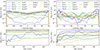 |
Fig. 8. Distribution and temporal evolution of the rms magnetic field at the stellar surface (r = R) of all the simulations. Upper panels: Poloidal (left) and toroidal (right) components of the azimuthally and temporally averaged rms-field as a function of latitude. Bottom panels: Temporal evolution of the horizontally (ϕθ) averaged poloidal (left) and toroidal (right) rms-field. |
The normalized power spectra of the velocity and magnetic field from a spherical harmonic decomposition (see Krause & Rädler 1980) of DipB is shown in the left panel of Fig. 9. The solid lines correspond to the power spectra of the first 15 years of the simulation, and the dashed lines of the last 15 years. It is clear that in both periods the magnetic power spectrum has its peak in the dipolar term with ℓ = 1. Moreover, during the early times, 99.54% of the magnetic energy is in the dipole component. At late times, this reduces to 97.27%, but this is not because the dipole amplitude decreases, but due to an increase in the contribution of smaller scales (ℓ > 1). The time evolution of the dipole amplitude (ℓ = 1), normalized by its initial value, is shown in the right panel of Fig. 9. In the cases with Dipole B and B*, the dipole amplitude is essentially constant over time, with the exception of DipBt* where the dipole decays more than in the other runs. Nevertheless, the fraction of the energy in the dipole changes from 99.33% at early to 94.19% at late times. In the runs with Dipole A, the dipole decays faster than in the rest of simulations. For example, in DipAt the dipole contains 98.98% of the energy at early times, but at the late times this fraction drops to 50.28%. This suggests that while Dipole B can enhance the dynamo and possibly land it on the strong field branch, Dipole A is not conduciveto this.
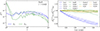 |
Fig. 9. Left panel: Normalized power spectra of the velocity |


4.3. Differential rotation
The averaged rotation rate is given by

where ϖ = r sin θ is the cylindrical radius. Additionally, the averaged meridional flow is
To quantify the amplitude of the radial and latitudinal differential rotation, we use the following parameters (Käpylä et al. 2013)
where rtop = 0.9R and rbot = 0.1R are the radius near the surface and center of the star, respectively. θeq is the latitude at the equator, and  is an average of
  between latitudes −θ and θ. Following Paper I, we define ΔΩCZ(r) and
  , which are the same as Eqs. (22) and (23), but with rtop = 0.2R and rbot = 0.05R, to study the differential rotation of the core.
The differential rotation parameters and the maximum meridional speeds are summarized in Table 3. From columns 3 and 4 of Table 3 we can conclude that MHDr2 already has an almost-rigid rotation close to the surface (see Fig. 8 of Paper I). However, the inclusion of a fossil field, irrespective of its type, reduces the amplitude of the differential rotation almost completely with typical values being  and
and  . A similar phenomena is observed in the convective core. In runs with Dipole A, the parameters of the core maintain their sign (
 ), which indicates that the solar-like state from run MHDr2 is still present in these simulations. However, the amplitude of these coefficients is weaker than in MHDr2. In the cases with Dipole B* and Dipole B, the differential rotation of the core is significantly quenched. The solar-like state changes to an anti-solar regime, where
  typically. This is also visible in the first three panels of Fig. 10. The initially retrograde column close to the axis of rotation (see panel (d) of Fig. 1) of MHDr2 changes to a weak prograde column in the runs with the enhanced dynamo. A similar transition was reported by Augustson et al. (2016), between their hydrodynamic and the superequipartition magnetic cases (see their Fig. 7). Moreover, our results are also in agreement with Featherstone et al. (2009), as the prominent retrograde columns of the progenitor cases are replaced by regions of slightly prograde rotation, and the radiative envelope is almost rotating solidly after the inclusion of a poloidal fossil field. Finally, from the last column of Table 3 we conclude that there is no apparent relation between β and the maximum meridional speeds.
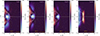 |
Fig. 10. Profiles of the temporally and azimuthally averaged rotation rate |

Differential rotation parameters and the maximum meridional flow  from all the simulations.
5. Discussion and conclusions
The interaction between the core dynamo of a 2.2 M⊙ A-type star and an imposed purely poloidal fossil field with a dipolar surface strength of 6 kG, was explored using star-in-a-box MHD simulations (Dobler et al. 2006; Käpylä 2021). Furthermore, as the observed magnetic fields from Ap stars are typically misaligned with their rotational axis, obliquity angles β between 0° and 90° were tested. In the case where none of the magnetic field lines are closed inside the star (Dipole A), the core dynamo does not seem to be affected, irrespective of the chosen inclination. A possible explanation for this, is that the internal poloidal field of this initial condition (Brmspol ≈ 6 kG) is too weak to excite a new dynamo mode. Moss (2004) found that an external poloidal magnetic field of the same order as the poloidal component of the initial dynamo, is sufficient to significantly affect the dynamo. Following this argument, the dipole field needs to be at least Brmspol = 19 kG (see Table 1) to change the nature of the core dynamo in our simulations, which is not achieved by Dipole A. In the cases where the magnetic field lines of the imposed field are closed inside the star (Dipole B and Dipole B*), Brmspol in this region is strong enough to affect the core dynamo. More specifically, with most of the explored inclinations (from 0° to 85°) the initially cyclic and hemispheric solutions of the dynamo changes to a mainly dipolar quasi-stationary configuration. The strength of this enhanced dynamo seems to be inversely related to the obliquity angle of the fossil field. The horizontal cases (β = 90°) start with the mentioned quasi-stationary solution, but decay after a few years, proving to be unstable. Inertia seems to play an important role in the geometry of the dynamo, that is, dipolar solutions are expected when inertia is weak (Christensen & Aubert 2006; Soderlund et al. 2012). This is in agreement with the enhanced dynamos, where Co ≈ 15, and where the addition of a strong dipole moves the simulation permanently to the dipolar branch. When inertia becomes relevant, multipolar solutions are expected. The runs in the dipolar branch by Gastine et al. (2012) have similar dipole-dominated solutions to the enhanced cases, while runs in the multipolar branch have a cyclic and hemispheric nature similar to MHDr2 (see their Fig. 12). The enhanced dynamos have superequipartition fields, such that Emag/Ekin is between 1.1 and 5.2. These ratios are comparable to the fast rotators of Augustson et al. (2016). However, we do not find fields as strong as those reported by Featherstone et al. (2009) in their mixed-case (Emag/Ekin ≈ 10).
In the enhanced cases, the strong magnetic fields affect the profiles of differential rotation, inducing nearly rigid rotation in the radiative envelope, and changing the differential rotation in the convective core from solar-like to anti-solar. A similar transition was reported by Featherstone et al. (2009) after the inclusion of a fossil field, and by Augustson et al. (2016) between the hydrodynamic and magnetic cases. It is worth mentioning that in the enhanced cases, the amplitude of the anti-solar differential rotation is much weaker than that from the original solar-like state. This is a direct consequence of magnetic quenching of differential rotation (see, e.g., Brun et al. 2004, 2005; Käpylä et al. 2017; Bice & Toomre 2023). Our results are in agreement with asteroseismic observations, as most of the observed intermediate-mass MS stars (M < 9 M⊙) have nearly solid body rotation (Kurtz et al. 2014; Bowman 2021, 2023).
Toroidal fields roughly comparable to the poloidal ones are found in the statistically steady state at the stellar surface. These fields are most likely transported from the enhanced core dynamo to the surface due to turbulent diffusion. In the relaxed state the surface magnetic field does not show signs of decay. In runs with Dipole B and B* the surface field has typically between 94% and 97% of its energy concentrated in the dipole mode. The relation between β and Brms is not prominent on the stellar surface (see right panels of Fig. 8), therefore, β seems to affect mostly the enhanced core dynamo. In Ap/Bp stars, the distribution of β seems to be random, with no apparent relation to the surface dipolar strength (Hubrig et al. 2007; Sikora et al. 2019; Shultz et al. 2019). The surface poloidal field strength is significantly weaker in simulations with horizontal dipoles than in the rest of cases.
The fossil fields were added after the saturation of the core dynamo. Nevertheless, all of the current cases with a sufficiently strong axial dipole land in a strong field branch where the dynamo mode changes from predominantly multipolar to dipolar. This coincides with results from other studies where the initial magnetic field was varied similarly (e.g., Gastine et al. 2012). In this work we explored very idealized tilted poloidal fields, roughly based on the observed large-scale magnetic fields of Ap/Bp stars. However, fossil fields coming from the PMS evolution could in principle have complex topologies. Unfortunately, very little is known about the geometries and topologies of Herbig Ae/Be stars, the progenitors of Ap/Bp stars (see e.g., Hubrig et al. 2020). A logical next step would be to model the PMS evolution of these stars, similarly to Emeriau-Viard & Brun (2017), but concentrating on Herbig Ae/Be stars. The obtained magnetic fields will probably become mainly dipolar during the main sequence, as shown by Braithwaite & Nordlund (2006), even random initial magnetic fields can potentially relax into a dipolar structure. However, how a more realistic configuration can affect an existing core dynamo remains unknown.
Data availability
Movie associated to Fig. 6 is available at https://www.aanda.org
Acknowledgments
JPH acknowledges financial support from ANID/DOCTORADO BECAS CHILE 72240057. DRGS gratefully acknowledges support by the ANID BASAL project FB21003 and the Alexander-von-Humboldt foundation. The simulations were performed with resources provided by the Kultrun Astronomy Hybrid Cluster via the projects Conicyt Quimal #170001, Conicyt PIA ACT172033, and Fondecyt Iniciacion 11170268. PJK acknowledges the stimulating discussions with participants of the Nordita Scientific Program on “Stellar Convection: Modelling, Theory and Observations” in August and September 2024 in Stockholm. CAOR acknowledges financial support from ANID (DOCTORADO DAAD-BECAS CHILE/62220030) as well as financial support from DAAD (DAAD/BECAS Chile, 2023 – 57636841 ). FHN acknowledges funding from the program Unidad de Excelencia María Maeztu, reference CEX2020-001058-M.
References
- Alecian, E., Wade, G. A., Catala, C., et al. 2013a, MNRAS, 429, 1001 [NASA ADS] [CrossRef] [Google Scholar]
- Alecian, E., Wade, G. A., Catala, C., et al. 2013b, MNRAS, 429, 1027 [Google Scholar]
- Alecian, E., Villebrun, F., Grunhut, J., et al. 2019, EAS Pub. Ser., 82, 345 [NASA ADS] [CrossRef] [EDP Sciences] [Google Scholar]
- Augustson, K. C., Brun, A. S., & Toomre, J. 2016, ApJ, 829, 92 [Google Scholar]
- Aurière, M., Wade, G. A., Silvester, J., et al. 2007, A&A, 475, 1053 [NASA ADS] [CrossRef] [EDP Sciences] [Google Scholar]
- Baryshnikova, I., & Shukurov, A. 1987, Astron. Nachr., 308, 89 [Google Scholar]
- Becerra, L., Reisenegger, A., Valdivia, J. A., & Gusakov, M. E. 2022, MNRAS, 511, 732 [NASA ADS] [CrossRef] [Google Scholar]
- Bernstein, I. B., Frieman, E. A., Kruskal, M. D., & Kulsrud, R. M. 1958, Proc. R. Soc. London Ser. A, 244, 17 [Google Scholar]
- Bice, C. P., & Toomre, J. 2023, ApJ, 947, 36 [NASA ADS] [CrossRef] [Google Scholar]
- Bowman, D. M. 2021, in OBA Stars: Variability and Magnetic Fields, 27 [Google Scholar]
- Bowman, D. M. 2023, Ap&SS, 368, 107 [NASA ADS] [CrossRef] [Google Scholar]
- Boyer, D. W., & Levy, E. H. 1984, ApJ, 277, 848 [NASA ADS] [CrossRef] [Google Scholar]
- Braithwaite, J. 2008, MNRAS, 386, 1947 [Google Scholar]
- Braithwaite, J. 2009, MNRAS, 397, 763 [NASA ADS] [CrossRef] [Google Scholar]
- Braithwaite, J., & Nordlund, Å. 2006, A&A, 450, 1077 [NASA ADS] [CrossRef] [EDP Sciences] [Google Scholar]
- Braithwaite, J., & Spruit, H. C. 2004, Nature, 431, 819 [Google Scholar]
- Brandenburg, A. 2017, A&A, 598, A117 [NASA ADS] [CrossRef] [EDP Sciences] [Google Scholar]
- Brandenburg, A., & Sarson, G. R. 2002, Phys. Rev. Lett., 88, 055003 [Google Scholar]
- Brandenburg, A., & Subramanian, K. 2005, Phys. Rep., 417, 1 [NASA ADS] [CrossRef] [Google Scholar]
- Briquet, M. 2015, Eur. Phys. J. Web Conf., 101, 05001 [Google Scholar]
- Brown, B. P., Oishi, J. S., Vasil, G. M., Lecoanet, D., & Burns, K. J. 2020, ApJ, 902, L3 [NASA ADS] [CrossRef] [Google Scholar]
- Browning, M. K., Brun, A. S., & Toomre, J. 2004, ApJ, 601, 512 [Google Scholar]
- Brun, A. S., Miesch, M. S., & Toomre, J. 2004, ApJ, 614, 1073 [Google Scholar]
- Brun, A. S., Browning, M. K., & Toomre, J. 2005, ApJ, 629, 461 [Google Scholar]
- Brun, A. S., Strugarek, A., Noraz, Q., et al. 2022, ApJ, 926, 21 [NASA ADS] [CrossRef] [Google Scholar]
- Buysschaert, B., Aerts, C., Bowman, D. M., et al. 2018, A&A, 616, A148 [NASA ADS] [CrossRef] [EDP Sciences] [Google Scholar]
- Cantiello, M., & Braithwaite, J. 2019, ApJ, 883, 106 [Google Scholar]
- Cantiello, M., Langer, N., Brott, I., et al. 2009, A&A, 499, 279 [NASA ADS] [CrossRef] [EDP Sciences] [Google Scholar]
- Charbonneau, P. 2020, Liv. Rev. Sol. Phys., 17, 4 [Google Scholar]
- Christensen, U. R., & Aubert, J. 2006, Geophys. J. Int., 166, 97 [NASA ADS] [CrossRef] [Google Scholar]
- Cowling, T. G. 1945, MNRAS, 105, 166 [NASA ADS] [CrossRef] [Google Scholar]
- Dobler, W., Stix, M., & Brandenburg, A. 2006, ApJ, 638, 336 [NASA ADS] [CrossRef] [Google Scholar]
- Donati, J. F., & Landstreet, J. D. 2009, ARA&A, 47, 333 [Google Scholar]
- Emeriau-Viard, C., & Brun, A. S. 2017, ApJ, 846, 8 [Google Scholar]
- Featherstone, N. A., Browning, M. K., Brun, A. S., & Toomre, J. 2009, ApJ, 705, 1000 [Google Scholar]
- Ferrario, L., Pringle, J. E., Tout, C. A., & Wickramasinghe, D. T. 2009, MNRAS, 400, L71 [NASA ADS] [CrossRef] [Google Scholar]
- Flowers, E., & Ruderman, M. A. 1977, ApJ, 215, 302 [Google Scholar]
- Gastine, T., Duarte, L., & Wicht, J. 2012, A&A, 546, A19 [NASA ADS] [CrossRef] [EDP Sciences] [Google Scholar]
- Grunhut, J. H., Wade, G. A., Neiner, C., et al. 2017, MNRAS, 465, 2432 [NASA ADS] [CrossRef] [Google Scholar]
- Hidalgo, J. P., Käpylä, P. J., Schleicher, D. R. G., Ortiz-Rodríguez, C. A., & Navarrete, F. H. 2024, A&A, 691, A326 [NASA ADS] [CrossRef] [EDP Sciences] [Google Scholar]
- Hubrig, S., Schöller, M., & Yudin, R. V. 2004, A&A, 428, L1 [NASA ADS] [CrossRef] [EDP Sciences] [Google Scholar]
- Hubrig, S., North, P., & Schöller, M. 2007, Astron. Nachr., 328, 475 [NASA ADS] [CrossRef] [Google Scholar]
- Hubrig, S., Schöller, M., Ilyin, I., et al. 2011, A&A, 536, A45 [NASA ADS] [CrossRef] [EDP Sciences] [Google Scholar]
- Hubrig, S., Järvinen, S. P., & Schöller, M. 2020, Azerbaijani Astron. J., 15, 68 [Google Scholar]
- Johansen, A., & Klahr, H. 2005, ApJ, 634, 1353 [NASA ADS] [CrossRef] [Google Scholar]
- Käpylä, P. J. 2021, A&A, 651, A66 [Google Scholar]
- Käpylä, P. J. 2022, ApJ, 931, L17 [CrossRef] [Google Scholar]
- Käpylä, P. J. 2024, A&A, 683, A221 [NASA ADS] [CrossRef] [EDP Sciences] [Google Scholar]
- Käpylä, P. J., Mantere, M. J., Cole, E., Warnecke, J., & Brandenburg, A. 2013, ApJ, 778, 41 [CrossRef] [Google Scholar]
- Käpylä, P. J., Käpylä, M. J., Olspert, N., Warnecke, J., & Brandenburg, A. 2017, A&A, 599, A4 [NASA ADS] [CrossRef] [EDP Sciences] [Google Scholar]
- Käpylä, P. J., Gent, F. A., Olspert, N., Käpylä, M. J., & Brandenburg, A. 2020, Geophys. Astrophys. Fluid Dyn., 114, 8 [CrossRef] [Google Scholar]
- Käpylä, P. J., Browning, M. K., Brun, A. S., Guerrero, G., & Warnecke, J. 2023, Space Sci. Rev., 219, 58 [CrossRef] [Google Scholar]
- Kholtygin, A. F., Akhnevsky, A. S., & Tsiopa, O. 2019, in Physics of Magnetic Stars, eds. D. O. Kudryavtsev, I. I. Romanyuk, & I. A. Yakunin, ASP Conf. Ser., 518, 83 [Google Scholar]
- Kochukhov, O., & Bagnulo, S. 2006, A&A, 450, 763 [NASA ADS] [CrossRef] [EDP Sciences] [Google Scholar]
- Kochukhov, O., & Wade, G. A. 2016, A&A, 586, A30 [NASA ADS] [CrossRef] [EDP Sciences] [Google Scholar]
- Kochukhov, O., Rusomarov, N., Valenti, J. A., et al. 2015, A&A, 574, A79 [NASA ADS] [CrossRef] [EDP Sciences] [Google Scholar]
- Korre, L., & Featherstone, N. A. 2024, ApJ, 964, 162 [NASA ADS] [CrossRef] [Google Scholar]
- Krause, F., & Rädler, K.-H. 1980, Mean-field Magnetohydrodynamics and Dynamo Theory (Oxford: Pergamon Press) [Google Scholar]
- Kurtz, D. W., Saio, H., Takata, M., et al. 2014, MNRAS, 444, 102 [Google Scholar]
- Landstreet, J. D., & Mathys, G. 2000, A&A, 359, 213 [NASA ADS] [Google Scholar]
- Landstreet, J. D., Bagnulo, S., Andretta, V., et al. 2007, A&A, 470, 685 [NASA ADS] [CrossRef] [EDP Sciences] [Google Scholar]
- Landstreet, J. D., Silaj, J., Andretta, V., et al. 2008, A&A, 481, 465 [NASA ADS] [CrossRef] [EDP Sciences] [Google Scholar]
- Lecoanet, D., Bowman, D. M., & Van Reeth, T. 2022, MNRAS, 512, L16 [NASA ADS] [CrossRef] [Google Scholar]
- Lyra, W., McNally, C. P., Heinemann, T., & Masset, F. 2017, AJ, 154, 146 [NASA ADS] [CrossRef] [Google Scholar]
- MacDonald, J., & Mullan, D. J. 2004, MNRAS, 348, 702 [NASA ADS] [CrossRef] [Google Scholar]
- MacGregor, K. B., & Cassinelli, J. P. 2003, ApJ, 586, 480 [NASA ADS] [CrossRef] [Google Scholar]
- Markey, P., & Tayler, R. J. 1973, MNRAS, 163, 77 [CrossRef] [Google Scholar]
- Markey, P., & Tayler, R. J. 1974, MNRAS, 168, 505 [NASA ADS] [CrossRef] [Google Scholar]
- Masada, Y., & Sano, T. 2014, ApJ, 794, L6 [Google Scholar]
- Mitra, D., Tavakol, R., Käpylä, P. J., & Brandenburg, A. 2010, ApJ, 719, L1 [Google Scholar]
- Moss, D. 2001, in Magnetic Fields Across the Hertzsprung-Russell Diagram, eds. G. Mathys, S. K. Solanki, & D. T. Wickramasinghe, ASP Conf. Ser., 248, 305 [Google Scholar]
- Moss, D. 2003, A&A, 403, 693 [NASA ADS] [CrossRef] [EDP Sciences] [Google Scholar]
- Moss, D. 2004, A&A, 414, 1065 [NASA ADS] [CrossRef] [EDP Sciences] [Google Scholar]
- Ortiz-Rodríguez, C. A., Käpylä, P. J., Navarrete, F. H., et al. 2023, A&A, 678, A82 [NASA ADS] [CrossRef] [EDP Sciences] [Google Scholar]
- Parker, E. N. 1979, Ap&SS, 62, 135 [NASA ADS] [Google Scholar]
- Paxton, B., Smolec, R., Schwab, J., et al. 2019, ApJS, 243, 10 [Google Scholar]
- Pencil Code Collaboration (Brandenburg, A.) et al. 2021, J. Open Source Software, 6, 2807 [CrossRef] [Google Scholar]
- Petitdemange, L., Marcotte, F., & Gissinger, C. 2023, Science, 379, 300 [NASA ADS] [CrossRef] [Google Scholar]
- Petitdemange, L., Marcotte, F., Gissinger, C., & Daniel, F. 2024, A&A, 681, A75 [NASA ADS] [CrossRef] [EDP Sciences] [Google Scholar]
- Pouquet, A., Frisch, U., & Léorat, J. 1976, J. Fluid Mech., 77, 321 [NASA ADS] [CrossRef] [Google Scholar]
- Prendergast, K. H. 1956, ApJ, 123, 498 [NASA ADS] [CrossRef] [Google Scholar]
- Raedler, K. H., & Braeuer, H. J. 1987, Astron. Nachr., 308, 101 [Google Scholar]
- Richard, O., Michaud, G., & Richer, J. 2001, ApJ, 558, 377 [Google Scholar]
- Rusomarov, N., Kochukhov, O., Ryabchikova, T., & Piskunov, N. 2015, A&A, 573, A123 [NASA ADS] [CrossRef] [EDP Sciences] [Google Scholar]
- Schleicher, D. R. G., Hidalgo, J. P., & Galli, D. 2023, A&A, 678, A204 [NASA ADS] [CrossRef] [EDP Sciences] [Google Scholar]
- Schneider, F. R. N., Ohlmann, S. T., Podsiadlowski, P., et al. 2019, Nature, 574, 211 [Google Scholar]
- Schuessler, M., & Paehler, A. 1978, A&A, 68, 57 [NASA ADS] [Google Scholar]
- Shorlin, S. L. S., Wade, G. A., Donati, J. F., et al. 2002, A&A, 392, 637 [NASA ADS] [CrossRef] [EDP Sciences] [Google Scholar]
- Shultz, M. E., Wade, G. A., Rivinius, T., et al. 2019, MNRAS, 490, 274 [NASA ADS] [CrossRef] [Google Scholar]
- Sikora, J., Wade, G. A., Power, J., & Neiner, C. 2019, MNRAS, 483, 3127 [NASA ADS] [CrossRef] [Google Scholar]
- Silvester, J., Kochukhov, O., Rusomarov, N., & Wade, G. A. 2017, MNRAS, 471, 962 [NASA ADS] [CrossRef] [Google Scholar]
- Soderlund, K. M., King, E. M., & Aurnou, J. M. 2012, Earth Planet. Sci. Lett., 333, 9 [Google Scholar]
- Spruit, H. C. 2002, A&A, 381, 923 [CrossRef] [EDP Sciences] [Google Scholar]
- Steenbeck, M., & Krause, F. 1969, Astron. Nachr., 291, 49 [NASA ADS] [CrossRef] [Google Scholar]
- Strugarek, A., Beaudoin, P., Charbonneau, P., & Brun, A. S. 2018, ApJ, 863, 35 [Google Scholar]
- Suárez Mascareño, A., Rebolo, R., & González Hernández, J. I. 2016, A&A, 595, A12 [Google Scholar]
- Tayler, R. J. 1973, MNRAS, 161, 365 [CrossRef] [Google Scholar]
- Waters, L. B. F. M. 2006, in Stars with the B[e] Phenomenon, eds. M. Kraus, & A. S. Miroshnichenko, ASP Conf. Ser., 355, 87 [Google Scholar]
- Waters, L. B. F. M., & Waelkens, C. 1998, ARA&A, 36, 233 [NASA ADS] [CrossRef] [Google Scholar]
- Wright, G. A. E. 1973, MNRAS, 162, 339 [Google Scholar]
- Yadav, R. K., Christensen, U. R., Morin, J., et al. 2015, ApJ, 813, L31 [Google Scholar]
All Tables
Differential rotation parameters and the maximum meridional flow from all the simulations.
All Figures
|
Fig. 1. Magnetic fields and flows from a snapshot of MHDr2 at t = 85 yr. Panels (a), (b): Radial and toroidal magnetic fields at the surface of the convective zone (r = 0.2R). Panel (c): Azimuthally averaged toroidal (colormap) and poloidal (arrows) magnetic fields. Panel (d): Azimuthally averaged toroidal flows (colormap) and meridional circulation (arrows). All the panels are clipped for a better display, and the minimum and maximum values are indicated below the colorbar. |
| In the text | |
|
Fig. 2. Imposed initial (fossil) magnetic fields in our simulations. The arrows represent the poloidal magnetic field lines, and the colormap the intensity of this component. Dipole A and Dipole B* are aligned to the rotational axis (β = 0°), and as an example of a misaligned dipole an inclination of β = 30° was added in Dipole B. The last panel corresponds to the initial snapshot of run DipB (Dipole B + MHDr2). |
| In the text | |
|
Fig. 3. Temporal evolution of the rms magnetic field in the convective core (r < 0.2R) from all simulations. The gray dashed line indicates 60 kG, which is the saturated value of the core dynamo from MHDr2. |
| In the text | |
|
Fig. 4. Time-latitude diagrams of the azimuthally averaged toroidal magnetic field |
| In the text | |
|
Fig. 5. Dynamo parameters cα = αΔr/ηturb and |
| In the text | |
|
Fig. 6. Azimuthally averaged toroidal magnetic field |
| In the text | |
|
Fig. 7. Same as Figure 4, but for runs without an enhanced dynamo. |
| In the text | |
|
Fig. 8. Distribution and temporal evolution of the rms magnetic field at the stellar surface (r = R) of all the simulations. Upper panels: Poloidal (left) and toroidal (right) components of the azimuthally and temporally averaged rms-field as a function of latitude. Bottom panels: Temporal evolution of the horizontally (ϕθ) averaged poloidal (left) and toroidal (right) rms-field. |
| In the text | |
|
Fig. 9. Left panel: Normalized power spectra of the velocity |
| In the text | |
|
Fig. 10. Profiles of the temporally and azimuthally averaged rotation rate |
| In the text | |
Current usage metrics show cumulative count of Article Views (full-text article views including HTML views, PDF and ePub downloads, according to the available data) and Abstracts Views on Vision4Press platform.
Data correspond to usage on the plateform after 2015. The current usage metrics is available 48-96 hours after online publication and is updated daily on week days.
Initial download of the metrics may take a while.