| Issue |
A&A
Volume 699, July 2025
|
|
|---|---|---|
| Article Number | A262 | |
| Number of page(s) | 13 | |
| Section | Stellar atmospheres | |
| DOI | https://doi.org/10.1051/0004-6361/202555073 | |
| Published online | 17 July 2025 | |
Unlocking the mystery of strontium synthesis in the early Galaxy through analysis of barium isotopes in very metal-poor stars★
1
Institute of Astronomy, Russian Academy of Sciences,
Pyatnitskaya 48,
119017
Moscow,
Russia
2
Goethe University Frankfurt, Institute for Applied Physics (IAP),
Max-von-Laue-Str. 12,
60438
Frankfurt am Main,
Germany
3
Heidelberger Institut für Theoretische Studien,
Schloss-Wolfsbrunnenweg 35,
69118
Heidelberg,
Germany
4
INAF, Osservatorio Astronomico di Trieste,
via Tiepolo 11,
34143
Trieste,
Italy
5
INFN, Sezione di Trieste,
via Valerio 2,
34134
Trieste,
Italy
6
Dipartimento di Fisica, Sezione di Astronomia, Università di Trieste,
Via G. B. Tiepolo 11,
34143
Trieste,
Italy
7
LIRA, Observatoire de Paris, Université PSL, Sorbonne Université, Université Paris Cité, CY Cergy Paris Université, CNRS,
92190
Meudon,
France
8
Zentrum für Astronomie der Universität Heidelberg, Astronomisches Rechen-Institut,
Mönchhofstr. 12,
69120
Heidelberg,
Germany
9
Department of Astronomy, University of Geneva,
Chemin Pegasi 51,
1290
Versoix,
Switzerland
★★ Corresponding author: sitamih@gmail.com
Received:
8
April
2025
Accepted:
5
June
2025
Aims. We determine the contributions of the rapid (r) and slow (s) neutron capture processes to the Ba isotope mixture, along with Ba, Eu, and Sr NLTE abundances, in a sample of very metal-poor stars. The selected stars formed before the contribution from the main s-process in low- and intermediate-mass stars became significant. Some of our sample stars are enhanced in Sr, with [Sr/Ba] reaching up to 0.7. These stars gained their high Sr abundance from a poorly understood process, sometimes referred to in the literature as a light element primary process, which may appear to be a weak s-process or a weak r-process. Our aim is to uncover the nature of this additional Sr source.
Methods. The abundances derived from the resonance Ba II 4554 and 4934 Å lines are influenced by the adopted Ba isotope mixture. We computed Ba isotope mixtures corresponding to different r- to s-process contributions (pure r-process, 80%/20%, 50%/50% and 12%/88%, i.e. solar ratio) and determined the corresponding abundances from the Ba II resonance lines in each sample star. Additionally, we determined Ba abundances from weak subordinate Ba II lines, which are unaffected by the adopted Ba isotope mixture. We then compared the Ba abundances derived from the subordinate lines with those from the Ba II resonance lines.
Results. We find a higher s-process contribution to Ba isotopes in stars with greater [Sr/Eu] and [Sr/Ba] overabundances, suggesting that the additional Sr synthesis was due to the early s-process occurring in massive stars. Using Sr-enhanced stars, we estimate the [Sr/Ba] ratio produced by the early s-process and obtain [Sr/Ba]earlyS = 1.1 ± 0.2. The derived value should be regarded as an upper limit, as we cannot definitively exclude the possibility of a contribution to Sr from the weak r-process, which produces Sr but not Ba. Regarding the potential synthesis of Sr and Ba in the i-process in massive stars, our results for Ba isotopes and element abundances argue that there was no detectable contribution from this process within the error bars in our sample stars.
Conclusions. In the early Galaxy, before significant main s-process enrichment, barium and strontium were produced primarily by the main r-process and the early s-process, which occurred in rapidly rotating massive stars.
Key words: stars: abundances / stars: atmospheres / Galaxy: evolution / Galaxy: halo
© The Authors 2025
 Open Access article, published by EDP Sciences, under the terms of the Creative Commons Attribution License (https://creativecommons.org/licenses/by/4.0), which permits unrestricted use, distribution, and reproduction in any medium, provided the original work is properly cited.
This article is published in open access under the Subscribe to Open model. Subscribe to A&A to support open access publication.
1 Introduction
The synthesis of light neutron-capture (n-capture) elements (Sr, Y, and Zr) has been puzzling astrophysicists for several decades. Detailed observational constraints on the origin of heavy elements and the early Galactic chemical evolution can be derived from spectroscopic studies of very metal-poor (VMP, [Fe/H]1 <−2) stars, which, as the oldest objects, provide a unique opportunity to study the earliest epoch of the Galaxy formation.
The literature data report a 2 dex spread in their [Sr/Ba] ratio, ranging from [Sr/Ba] = −0.4 in stars where n-capture elements originate purely from the main rapid (r) n-capture process (Sneden et al. 2003; Barklem et al. 2005; Hayek et al. 2009; Mashonkina et al. 2010; Roederer et al. 2018; Shah et al. 2024), up to a high [Sr/Ba] of 1.5 dex (see, for example, pioneering studies and some more recent work by Spite & Spite 1978; Gratton & Sneden 1994; McWilliam et al. 1995; Mashonkina & Gehren 2001; Aoki et al. 2005; François et al. 2007; Sneden et al. 2008; Roederer 2013; Hansen et al. 2012, 2014, and many others studies). This suggests the presence of an additional source of light n-capture elements beyond the main r-process. The main slow (s) n-capture process does not fit this role, as it occurs in asymptotic giant branch (AGB) stars with masses from 1 to 6 M⊙, and its contribution to the Galactic chemical evolution becomes significant after a delay of at least 1 Gyr, detectable in stars with [Fe/H] >−2 (Travaglio et al. 2004; Simmerer et al. 2004; Käppeler et al. 2011; Kobayashi et al. 2020).
The need for an additional source of light n-capture elements operating in the early epoch of Galactic chemical evolution was first postulated by Travaglio et al. (2004), and it was named the light element primary process (LEPP). However, the LEPP was introduced as a phenomenological process without any specific hypotheses regarding its astrophysical site or nucleosynthesis mechanism. The nature and nucleosynthesis mechanism of this extra source of the light trans-iron elements remain debated. However, it is generally believed to be linked to massive stars, as they evolved rapidly and began to enrich the interstellar gas at the earliest phases of Galactic chemical evolution. Several hypotheses have been proposed for the source associated with the s-process. This includes the weak s-process in massive stars during the hydrostatic core He-burning phase (Raiteri et al. 1991b) and the shell carbon-burning phase (Raiteri et al. 1991a), as well as the s-process in fast-rotating, extremely metal-poor (EMP, [Fe/H] ≤ −3) massive stars (Pignatari et al. 2008; Chiappini et al. 2011; Cescutti et al. 2013; Cescutti & Chiappini 2014; Rizzuti et al. 2021) occurring in the same phases. For observers, a key difference between the above predictions is that models incorporating stellar rotation predict the production of the second-peak s-process elements (Ba, Ce, La, etc.), whereas standard weak s-process models stop at the first-peak s-process elements (Sr, Y, Zr). The s-process models in massive stars have been explored across a wide range of masses, metallicities, and rotational velocities (Frischknecht et al. 2012, 2016; Choplin et al. 2018; Limongi & Chieffi 2018). A key signature of the s-process is the production of even Ba isotopes 134Ba and 136Ba, which are s-process-only isotopes. Consequently, the chemical evolution model of Cescutti et al. (2013) and Cescutti & Chiappini (2014) predicts that VMP stars with high [Sr/Ba] should exhibit an enhanced value of the even isotopes. This results from their formation from s-process material produced by rapidly rotating massive stars.
Other proposed scenarios include the following: charged-particle reactions in the high-entropy wind of young neutron stars (Woosley & Hoffman 1992; Qian & Wasserburg 2007); the weak r-process in core collapse supernovae (Izutani et al. 2009; Arcones & Bliss 2014); the νp-process in proton-rich supernovae ejecta (Fröhlich et al. 2006; Eichler et al. 2018; Ghosh et al. 2022); the intermediate n-capture process (i-process, Cowan & Rose 1977) in low-metallicity AGB stars with masses below 4 M⊙ (Choplin et al. 2021, 2024); and the i-process in massive VMP stars (Banerjee et al. 2018). These processes, except for the i-process, produce Sr but not Ba, while the i-process yields both Sr and Ba, with a predominance of odd barium isotopes 135Ba and 137Ba (Choplin et al. 2024). However, the i-process struggles to explain VMP stars with high [Sr/Ba]: the first scenario (Choplin et al. 2024) is attributed to low- and intermediate-mass stars, which enrich the interstellar gas with a delay, while the second one (Banerjee et al. 2018) does not efficiently produce Sr, predicting close to or below solar [Sr/Ba] ratios.
To better understand the source of additional Sr, we aim to answer (i) whether the source of extra Sr is the s-process or r-process, (ii) whether this source produces a significant amount of Ba, and (iii) which Ba isotopes are formed. Our key diagnostics for identifying the n-capture element sources are: (i) [Ba/Eu] as a proxy for r-process contribution; (ii) [Sr/Ba] as a tracer of the extra Sr production source in the earliest epoch; and (iii) the Ba isotope ratio as a key indicator distinguishing between the s- and r-process.
The paper is structured as follows. In Sect. 2, we describe our sample stars and observations. The abundance determination method is presented in Sect. 3. A discussion of our findings is provided in Sect. 4, and our conclusions are summarised in Sect. 5.
2 Stellar sample and observations
Our sample consists of 16 VMP giant stars from the Chemical Evolution of R-process Elements in Stars (CERES) survey (Lombardo et al. 2022, hereafter LB22). The selected stars have normal carbon abundances (Fernandes de Melo et al. 2024), and their chemical composition is typical to the Milky Way (MW) halo stars with the corresponding metallicity. The majority of the sample stars fall within a metallicity range of −3.10 < [Fe/H] <−2.45, with one star having [Fe/H] = −2.15. Regarding the origin of the n-capture elements in the sample stars, they either have [Ba/H] <−2.4 (Lombardo et al. 2025, hereafter LH25) and formed before the contribution from the main s-process in lowand intermediate-mass stars became significant (Simmerer et al. 2004, LH25), or they are r-process enhanced stars with −2.4 < [Ba/H] <−2.2. Three of the sample stars are strongly r-process-enhanced r- II type stars with [Eu/Fe]2 = 1.3, while seven stars are r- I type, with 0.3 < [Eu/Fe] < 0.8. Thus, the selected stars trace the earliest epoch of Galactic chemical evolution and n-capture element synthesis.
For Ba isotope ratio analysis, we selected stars with high-resolution observed spectra covering both Ba II resonance lines at 4554 Å and 4934 Å. Additionally, the equivalent widths (EWs) of these lines should not exceed 140 mÅ. Sixteen of the fifty-two CERES stars meet these criteria, with their Ba II resonance line EWs ranging from 42 mÅ to 135 mÅ. The selected stars, along with their stellar atmosphere parameters, are listed in Table 1. Our selection criteria provide a suitable stellar sample, where the Ba II resonance lines are strong enough to trace Ba isotope ratios while remaining unsaturated enough to allow for accurate abundance measurements.
For our sample stars, high-resolution spectra were obtained by LB22 with the UV-Visual Echelle Spectrograph (UVES) at the UT2 Kueyen Telescope, with high signal-to-noise (S/N) ratios >150 per pixel at 3900 Å. Details of the individual LB22 spectra, including S/N ratio, spectral resolution, exposure time, observation date, and settings, are provided in Table A.1 of LB22. The LB22 spectra cover a wide wavelength range and allow us to analyse the lines of Ba II at 5853 Å, 6141 Å, 6494 Å, and 4934 Å, but not the Ba II 4554 Å line, due to a wavelength gap between 4520 Å and 4780 Å. Therefore, in this study, we complement the observations from LB22 with additional spectra covering the Ba II 4554 Å line, obtained either with UVES or the High-Resolution Echelle Spectrometer (HIRES) at the Keck I Telescope. The adopted spectra are of high quality, with a spectral resolution of λ/Δλ > 40 000 and a signal-to-noise ratio of S/N > 100. These spectra are available from the European Southern Observatory Science Archive and the Keck Observatory Archive, respectively. The proposal IDs and PIs for the spectra used in the Ba II 4554 Å analysis are listed in Table 1.
Stellar sample, atmospheric parameters, and characteristics of the observed spectra used for the Ba II 4554 Å line analysis.
3 Abundance analysis
3.1 Codes and model atmospheres
In this study, we used classical 1D model atmospheres from the MARCS model grid (Gustafsson et al. 2008), interpolated for the given Teff, log g, and [Fe/H] of the stars, while atlas 12 model atmospheres (Kurucz 2005) were adopted in the CERES project (LB22 and LH25). We verified that using either MARCS or ATLAS 12 models yields consistent results.
We solved the coupled radiative transfer and statistical equilibrium equations using the DETAIL code (Giddings 1981; Butler 1984), incorporating the updated opacity package presented by Mashonkina et al. (2011). For synthetic spectra calculations, we used the SYNTHV_NLTE code (Tsymbal et al. 2019), attached to the IDL BINMAG code (Kochukhov 2018). This method allowed us to obtain the best fit to the observed line profiles while accounting for the non-local thermodynamic equilibrium (NLTE) effects via pre-calculated departure coefficients (the ratio between NLTE and LTE atomic level populations) for a given model atmosphere. When fitting the line profiles, the abundance of the element of interest was varied alongside the macroturbulent velocity (vmac) and the radial velocity (vr).
The spectral synthesis line list was extracted from a recent version of the Vienna Atomic Line Database (VALD, Pakhomov et al. 2019; Ryabchikova et al. 2015), which provides isotopic and hyperfine structure components for a number of studied chemical elements. We adopted the oscillator strengths recommended by VALD.
3.2 Atmospheric parameters and impact of their uncertainties on abundance determination
The selected sample stars are VMP giants with parallaxes ranging from 0.17 to 7.63 mas (Gaia Collaboration 2021). Photometric effective temperatures (Teff) and distance-based surface gravities (log g) are adopted from LB22. The uncertainty in Teff is 100 K, and the uncertainty in log g amounts to 0.08 dex. In this study, we focused on the analysis of Ba II lines and the comparison of barium abundances derived from the resonance (strong) and subordinate (weak) lines.
The uncertainties in Teff and log g affect abundances from different Ba II lines in the same way and do not significantly impact the abundance difference between the resonance and subordinate lines of Ba II. For example, in a model atmosphere with Teff/log g/[Fe/H] = 5100/2.46/−2.5, a shift in Teff of 100 K results in an abundance shift of 0.10 and 0.07 dex for the Ba II 4554 Å and 5853 Å lines, respectively, with EWs of 120 mÅ and 25 mÅ. Overall, this shift in Teff produces a minor effect of 0.03 dex on the abundance difference between the two lines. In the same model atmosphere, a change in log g of 0.08 dex results in a similar abundance shift of 0.03 dex for both lines and does not affect the abundance difference.
Regarding variations in the microturbulent velocity (ξt), an uncertainty of 0.2 km s−1 has a significant effect on the abundance derived from the resonance line, causing a shift of 0.10 dex, while the corresponding shift for the Ba II 5853 Å line is negligible. In our sample stars, the EWs of the Ba II resonance lines vary from 60 to 130 mÅ. For the weaker Ba II resonance line, with EW4554 of 60 mÅ, an uncertainty in ξt of 0.2 km s−1 results in an abundance shift of 0.04 dex.
3.3 Determination of ξt
LB22 relies on ξt calculated using an empirical formula provided in Mashonkina et al. (2017a, hereafter MJ17). The adopted formula was derived from ξt determinations based on Fe I and Fe II lines in a sample of VMP giants and provides an accuracy of 0.2 km s−1. In our study, the uncertainty in ξt is crucial, since it mostly contributes to an uncertainty in barium abundance from the resonance lines. We refine ξt using Ti II lines and adopt ξt values that yield consistent titanium abundances from Ti II lines with different EWs.
Unlike the conventional use of iron lines for ξt determinations, we selected Ti II lines because they have accurate oscillator strengths based on the laboratory measurements of Wood et al. (2013), exhibit minimal NLTE effects, and are convenient to use. The strongest lines of Ti II are of comparable strength to the Ba II resonance lines in the corresponding model atmospheres. For example, in the case of the Ba II 4554 Å line, the equivalent widths are EW4554 = 60 mÅ and 124 mÅ, for HE0336–2412 and HD 27928, respectively. For the Ti II 4468 Å line, the equivalent widths are EW4417 = 85 mÅ and 109 mÅ in the same two stars, respectively.
Although the NLTE effects for Ti II are not large (Bergemann 2011; Sitnova et al. 2016; Mallinson et al. 2022), they are not negligible. We account for deviations from LTE using the Ti I- II model atom from Sitnova et al. (2016), updated with data for inelastic collisions with hydrogen atoms (Ti II +H) based on quantum-mechanical calculations presented in Sitnova et al. (2020). A grid of NLTE abundance corrections (the difference between NLTE and LTE abundance) for Ti II lines covering our stellar parameter range is provided in Table 2. For each sample star, we select the microturbulent velocity that provides consistent abundances from weak and strong Ti II lines, with abundance slopes as a function of EW of ≤10−4 dex per mÅ.
When comparing the derived ξt values with those calculated from the empirical formula of MJ17, we find slightly lower values, with the difference never exceeding 0.25 km s−1. For CES1427–2214, the star with the largest revision in ξt (0.25 km s−1), we show the NLTE abundances from Ti II as a function of EW for ξt calculated using the MJ17 formula and those derived from Ti II lines (Fig. 1). Using ξt = 1.85 km s−1 results in a significant trend in both NLTE and LTE, with slopes of −2.0 · 10−3 and −1.3 · 10−3 dex per mÅ, respectively. In contrast, a ξt value lower by 0.25 km s−1 results in consistent abundances from Ti II lines of different strengths, with slopes of −5 · 10−5 and 6 · 10−4 dex per mÅ in NLTE and LTE, respectively. For CES1427–2214, we ensured that the ξt derived from Ti II lines yielded consistent NLTE abundances from Fe I and Fe II lines of different strength (Fig. 1, bottom panel). See MJ17 for the line list and the NLTE method of iron abundance determination.
Observations show that stars with higher log g have lower ξt (see, for example, the empirical formula for ξt derived for dwarfs and subgiants in Sitnova et al. 2015). The majority of our sample stars are giants at the base of the RGB, with log g ≃ 2.5, whereas the stellar sample of MJ17 consists mostly of cool giants, with 45 out of 59 stars having log g less than 2.0. The difference in stellar parameters between our sample and the stars used to derive the empirical formula may explain the slightly lower ξt values obtained in this study. We find systematically lower ξt values in stars with higher log g, whereas consistent ξt values are obtained for the four stars with log g <2.0.
Using our new measurements, we derived an empirical formula suitable for ξt determination in giants at the base of the RGB: ξt = −1.12 + 8.37 · 10−4 · Teff − 6.48 · 10−1 · log g.
Here, we assume that ξt does not depend on [Fe/H], as the corresponding coefficients in the MJ17 and Sitnova et al. (2015) formulae are small and have opposite signs, suggesting no significant correlation between ξt and [Fe/H]. When comparing ξt measurements for individual stars with predictions from the above formula, we find that the difference does not exceed 0.10 km s−1 in absolute value, with a standard deviation of 0.05 km s−1.
NLTE abundance corrections and EWs in mÅ for Ti II lines as a function of Teff, log g, and [Fe/H].
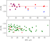 |
Fig. 1 Top panel: NLTE abundances from Ti II lines in CES1427–2214 as a function of the EW computed for ξt = 1.60 km s−1 (squares) and 1.85 km s−1 (circles). Bottom panel: NLTE abundances from Fe I (triangles) and Fe II (asterisks) lines in CES1427–2214 computed for ξt = 1.60 km s−1. |
3.4 Analysis of the Bair lines
We analysed five lines of Ba II: the strong resonance lines at λ = 4554 Å and 4934 Å, and the subordinate lines at λ = 5853 Å, 6141 Å, and 6496 Å. There is a Fe I 4934.0 Å line with a lower level energy of Eexc = 4.15 eV and an oscillator strength of log gf = −0.58 in the blue wing of the Ba II 4934.1 Å line. Fifteen of our sample stars have [Fe/H] ≤ −2.4, and blending with the Fe I 4934.0 Å line is negligible. For the most metal-rich sample star, HD 128279 (CES1436–2906), with [Fe/H] = −2.15, we show the observed spectrum around the Ba II 4934.1 Å line, along with synthetic spectra calculated with and without the iron line (Fig. 2).
The subordinate line Ba II 6141.71 Å is blended with the Fe I 6141.73 Å line, which has Eexc = 3.60 eV and log gf = −1.46. We accounted for this line in our spectrum synthesis using the iron abundance derived in LB22. For the most metal-rich star, varying the iron abundance within an uncertainty of 0.13 dex (LB22) results in negligible changes in the synthetic spectrum and does not affect barium abundance determination.
3.4.1 NLTE effects
To account for departures from LTE, we adopted the Ba II model atom from Mashonkina & Belyaev (2019). The NLTE effects for Ba II are moderate, leading to either weaker or stronger lines compared to LTE, depending on the line strength and stellar atmosphere parameters. In our sample stars, NLTE abundance corrections for individual Ba II lines do not exceed 0.13 dex in absolute value.
We draw attention to an intriguing line formation phenomenon observed for the Ba II resonance line in some stars. Based on the ratio of the oscillator strengths of the Ba II 4934 Å and Ba II 4554 Å lines (f4934/f4554 = 0.60), one might expect a similar ratio for their corresponding EWs, assuming the spectral lines lie within the linear portion of the curve of growth. Although our lines are stronger and extend beyond the linear portion, in the three stars with the weakest Ba II lines, the ratio EW4934/EW4554 is approximately 0.7. Notably, this ratio increases for stronger Ba II lines, though it never reaches unity in LTE. In seven of our sample stars with strong resonance lines (EW > 110 mÅ), the Ba II 4554 Å and Ba II 4934 Å lines have nearly the same strength, and in four of them, the EW of the Ba II 4934 Å line slightly exceeds that of the Ba II 4554 Å line.
When Ba II resonance lines are stronger than ≃100 mÅ, NLTE leads to stronger lines compared to LTE, and the NLTE abundance corrections are negative. For the Ba II 4934 Å line, NLTE corrections are larger in absolute value than for the Ba II 4554 Å line. This paradox is explained by the fact that the NLTE effects for the Ba II 4934 Å line result in more efficient line strengthening compared to the Ba II 4554 Å line. Figure 3 shows the departure coefficients for the ground state of Ba II (6s) and the upper levels of the resonance transitions in a model atmosphere of a VMP giant. The Ba II 4554 Å and 4934 Å lines form in the 6s– 6p (J = 3/2) and 6 s– 6 p (J = 1/2) transitions, respectively.
Strong resonance lines form across a broad atmospheric depth range, up to logτ5000 = −2.1. In the high atmospheric layers, the upper levels are underpopulated relative to LTE and to the ground state, and the ratio Sν/Bν ~ bup/blow < 1, where Sν and Bν are the line source function and the Planck function, respectively. A decrease in the line source function results in a lower flux and a stronger line core compared to LTE. In deeper atmospheric layers with logτ5000 > − 1, the situation is reversed: radiative pumping in the resonance transition results in a relative overpopulation of the upper levels relative to the ground state, and weakening the line compared to LTE. This effect is smaller for the Ba II 4934 Å line, which has a lower oscillator strength than the Ba II 4554 Å line. Due to the reduced line weakening in the deep layers, the Ba II 4934 Å line may ultimately appear stronger than the Ba II 4554 Å line.
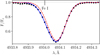 |
Fig. 2 Ba II 4934 Å line profile in the observed spectrum (circles) of the most metal-rich sample star CES1436–2906 with [Fe/H] = −2.15 along with a synthetic best-fit NLTE spectrum (solid line) and a spectrum, calculated neglecting the Fe I 4934 Å line (dashed line). |
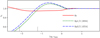 |
Fig. 3 Departure coefficients of the ground state of Ba II (6s) and the upper levels of the resonance transitions in a model atmosphere of a VMP giant. The vertical dashes indicate the line core formation depths of the resonance lines of different strength: 130 mÅ and 60 mÅ at logτ5000 = −2.1 and −1.2, respectively. |
3.4.2 Impact of Ba isotope ratio on abundance determination
Barium abundance in stars can be represented by up to five isotopes: 134Ba, 135Ba, 136Ba, 137Ba, and the most abundant isotope, 138Ba. The isotopes 134Ba and 136Ba are s-only isotopes and cannot be produced in the r-process due to the presence of the stable r-only isotopes 134Xe and 136Xe, which block the β-decay path and prevent the formation of 134Ba and 136Ba (Rolfs et al. 1987).
Odd isotopes are subject to hyperfine splitting (HFS) of the energy levels, and a higher fraction of odd isotopes results in a broader line profile and greater total absorbed energy. The HFS primarily affects the ground state, meaning that Ba II resonance lines can serve as a diagnostic of the Ba isotope ratio. In contrast, subordinate lines are unaffected by the adopted isotope ratio and can be used as reliable indicators of barium abundance. By determining the abundance from subordinate lines, one can infer the Ba isotope ratio, which can then be translated into the relative contributions of the r- and s-processes. The idea of estimating the r/s mixture of a star was first proposed by Cowley & Frey (1989), who pointed out the importance of accounting for HFS in Ba abundance determinations. This method has been applied to MP stars in the MW (Mashonkina & Zhao 2006; Mashonkina et al. 2008; Mashonkina & Belyaev 2019) and the Sculptor dwarf spheroidal (dSph) galaxy (Jablonka et al. 2015).
Magain & Zhao (1993) and Magain (1995) suggested a different method based on measuring the broadening of the Bail resonance lines and applied it to the VMP star HD 140283. Depending on the quality of the observed spectrum and the adopted line formation calculation method, different authors report different results for Ba isotope origin in HD 140283: a pure r-process in 1D LTE (Magain & Zhao 1993; Magain 1995), a solar mixture in 1D LTE (Lambert & Allende Prieto 2002) and in 3D LTE (Collet et al. 2009), a pure s-process in 1D LTE (Gallagher et al. 2010), and a mostly r-process in 3D LTE (Gallagher et al. 2015).
For barium, we determined abundances using different isotope ratios corresponding to the following r- to s-process fractions: 100%/0% (pure r-process), 80%/20%, 50%/50%, 12%/88% (solar), and 0%/100% (pure s-process). We adopted s-process and r-process residual Ba isotope yields from Prantzos et al. (2020). A larger r-process fraction results in a higher proportion of odd isotopes and a lower abundance derived from the resonance lines compared to that obtained with a lower r-process fraction. For each star, we provided abundances from individual spectral lines along with their measured EWs (Table 3).
Figure 4 illustrates the impact of the adopted Ba isotope mixture on barium abundance derived from the resonance lines. We plot the abundances from Ba II 4554 Å and 4934 Å lines in two sample stars: one with the weakest lines (HE0336–2412/CES0338–2402) and another with the strongest lines (r- II type star HE2327–5642/CES2330–5626). The stronger the Ba II resonance lines, the more sensitive their abundances are to the adopted Ba isotope mixture. For example, for the Ba II 4554 Å line with EW = 59 mÅ, the abundance difference between pure r- and pure s-process Ba isotope mixtures is 0.30 dex. The corresponding difference in HE2327–5642, where EW4554 = 133 mÅ, amounts to 0.34 dex. Notably, in HE2327–5642, the Ba II 4934 Å line is slightly more sensitive to the Ba isotope mixture, as it is slightly stronger than the Ba II 4554 Å line due to the effect discussed earlier.
The adopted Ba isotope mixture has a significant impact on the abundance derived from resonance lines, while the observed line profiles can be fitted when adopting any Ba isotope mixture. To demonstrate the quality of spectral fitting, we selected the UVES spectrum of HE0336–2412 (CES0338–2402), which has a spectral resolution of R = 107 200, higher than that of most sample stars, whose spectra were observed at R ≃45 000. Since HE0336–2412 has one of the weakest Ba II 4554 Å lines (EW = 59 mÅ), we also include the spectrum of HD 27928 (CES0422–3715) with EW4554 = 124 mÅ, obtained using HIRES with R = 47 700 (Fig. 5). For illustration, we present the best-fit synthetic NLTE spectra of the Ba II 4554 Å line computed with pure r-process and pure s-process Ba isotope ratios. Regardless of whether an r- or s-process Ba isotope mixture is used, we achieve a satisfactory fit to the observed spectra.
For CES0338–2402, the best-fit spectrum parameters are log ε(Ba)/vmac = −1.24/3.6 km s−1 (pure r-process) and −0.94/4.2 km s−1 (pure s-process). The corresponding values for CES0422–3715 are log ε(Ba)/vmac = −0.30/3.0 km s−1 and 0.07/3.3 km s−1. In our abundance determination method, vmac is treated as a free parameter when fitting individual spectral lines. From analysis of different spectral lines in a given star, we estimate a typical uncertainty in vmac as 2 km s−1. This uncertainty prevents us from determining the Ba isotope mixture solely from the Ba II resonance line profiles.
NLTE and LTE abundances and EWs of Ba II lines in the sample stars.
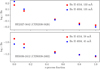 |
Fig. 4 NLTE abundances from the Ba II 4554 Å and 4934 Å lines as a function of r-process contribution to Ba isotopes in the two sample stars. The EWs of the resonance lines are indicated. |
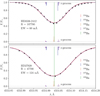 |
Fig. 5 Top panel: Ba II 4554 Å line profile in the observed spectrum (circles) of HE0336–2412 (CES0338–2402). Synthetic best-fit NLTE spectra, derived using pure r-process (dashed line) and pure s-process (dotted line) Ba isotope mixtures are almost indistinguishable, demonstrating that a reasonable fit can be achieved with any adopted isotope ratio. Vertical dashes show the relative contribution of different Ba isotopes to the r-process and s-process; see legend for designations. Bottom panel: Same as the top panel for HD 27928 (CES0422–3715). |
NLTE and LTE abundances and EWs from individual Sr II and Eu II lines in the sample stars.
NLTE abundance ratios and Ba odd isotope fractions of sample stars.
3.5 Sr and Eu abundances
We determined Sr abundances from the Sr II 4077 Å and 4215 Å lines (Table 4.) To account for the NLTE effects, we relied on the Sr II model atom presented in Mashonkina et al. (2022) and the NLTE abundance corrections from the INASAN database3 (Mashonkina et al. 2023). There are two reasons why we determined Sr abundances in this study instead of taking them from LB22. First, for six of the selected sample stars, Sr abundances are missing in LB22. Secondly, a revision in ξt affects the Sr II lines, as they are strong in our sample stars, and Sr abundances might be up to 0.2 dex higher than those computed with the ξt from the MJ17 formula.
We determined Eu abundances in our sample stars using the Eu II model atom of Mashonkina & Gehren (2000). LH25 relies on the Eu II 3819 Å and 4129 Å lines. The first of these is difficult to analyse, as this line is located in the blue wing of a strong Fe I 3819.62 Å line and, in addition, its blue wing is blended with the Cr I 3819.56 Å line. In stars with weak Eu lines, the above uncertainty, along with the uncertainty in the continuum placement, results in a systematically lower abundance from the Eu II 3819 Å compared to that from the Eu 4129 Å line. Instead of this line, we included in our analysis the Eu II 4205 Å line, which is free of blending in the metallicity range we deal with in this study. The average Eu abundances are calculated from Eu II 4129 Å and 4205 Å lines. Three of the sample stars have very weak lines of Eu II with EW < 6 mÅ, and we used their Eu abundances with caution. These measurements are marked with a < symbol in Table 5.
3.6 Element abundances and uncertainties
Table 5 presents the NLTE abundance ratios and fractions of odd Ba isotopes Fodd = (N(135Ba)+N(137Ba))/N(Ba). We adopted the following solar abundances from Lodders (2021): log ε(Sr)⊙ = 2.88, log ε(Ba)⊙ = 2.17, and log ε(Eu)⊙ = 0.51.
Uncertainties in [X/H] ratios were computed, including uncertainties in stellar atmosphere parameters along with the dispersion of the single line measurements around the mean ![$\[\sigma_{\text {st }}=\sqrt{\Sigma\left(\log~ \varepsilon-\log~ \varepsilon_{i}\right)^{2} /(N-1)}\]$](/articles/aa/full_html/2025/07/aa55073-25/aa55073-25-eq14.png) , where N is the total number of lines. For our Sr, Ba, and Eu abundance determination, we assume that the dispersion and the systematic uncertainties caused by variations in stellar parameters are uncorrelated. This assumption is valid since, for each of the studied elements, their spectral lines belong to the same species, have nearly the same intensity, and originate from atomic levels with similar or identical Eexc. Therefore, changes in Teff, log g, and ξt do not contribute to line-to-line scatter, allowing the total abundance ratio [X/H] uncertainty, to be calculated as follows:
, where N is the total number of lines. For our Sr, Ba, and Eu abundance determination, we assume that the dispersion and the systematic uncertainties caused by variations in stellar parameters are uncorrelated. This assumption is valid since, for each of the studied elements, their spectral lines belong to the same species, have nearly the same intensity, and originate from atomic levels with similar or identical Eexc. Therefore, changes in Teff, log g, and ξt do not contribute to line-to-line scatter, allowing the total abundance ratio [X/H] uncertainty, to be calculated as follows:
![$\[\sigma_{[\mathrm{X} / \mathrm{H}]}^2=\sigma^2(X)+\sigma^2\left(T_{\mathrm{eff}}\right)+\sigma^2(\log g)+\sigma^2\left(\xi_{\mathrm{t}}\right).\]$](/articles/aa/full_html/2025/07/aa55073-25/aa55073-25-eq15.png)
When computing abundance ratios [X/Y], where X and Y are Sr, Ba, and Eu, we neglected the uncertainty in log g, since a shift in log g produces the same abundance shift for the above elements. The corresponding uncertainties caused by changes in Teff and ξt are reduced compared to those for absolute abundances, since changes in these parameters affect the Sr II, Ba II, and Eu II spectral lines in the same way. For abundance ratios X and Y, the uncertainty in their ratio is calculated as follows:
![$\[\sigma_{[\mathrm{X} / \mathrm{Y}]}^2=\sigma^2(X)+\sigma^2(Y)+\sigma^2\left(\Delta T_{\mathrm{eff}}\right)+\sigma^2\left(\Delta \xi_{\mathrm{t}}\right).\]$](/articles/aa/full_html/2025/07/aa55073-25/aa55073-25-eq16.png)
4 Discussion
4.1 Abundance trends
Figure 6 shows the [Sr/Ba] ratio as a function of [Ba/Eu] in our sample stars. The [Ba/Eu] ratio ranges from −0.87 in an r- II type star to −0.36 in a star with low Eu abundance. Three r- II sample stars exhibit consistently low [Ba/Eu] values, with an average ratio of [Ba/Eu]r = −0.81 ± 0.05, which aligns with the pure r-process ratio predictions [Ba/Eu]r = −0.8 (Bisterzo et al. 2014), −0.9 (Prantzos et al. 2020), −0.7 (Arlandini et al. 1999), and an empirical ratio [Ba/Eu]r = −0.87 ± 0.06 based on NLTE analysis of r- II stars (Mashonkina & Christlieb 2014). The [Sr/Ba] ratio spans a wide range, from [Sr/Ba]r = −0.31 ± 0.02 in r- II stars to a maximum of 0.74.
Figure 7 presents the abundance difference between the subordinate and resonance lines, ΔBa (sub.-res.), computed with different r- to s-process fractions (100%/0%, 80%/20%, 50%/50%, and 12%/88%) as a function of abundance ratios. We observe an increasing trend: the fraction of Ba even isotopes rises with [Ba/Eu], suggesting an increasing s-process contribution. It is unsurprising that the s-process produces Ba even isotopes and results in an increasing [Ba/Eu]. The key point is that an increasing trend is also observed when plotting ΔBa (sub.-res.) against [Sr/Eu] and [Sr/Ba] (Fig. 7, middle and bottom panels). This supports the idea of a common synthesis of additional Sr (beyond that produced via the main r-process) and Ba even isotopes, implying that the extra Sr originates from the s-process. This, in turn, clearly indicates that Sr and Ba are co-produced in this source. We do not claim that this was the only source, however, its contribution to Sr synthesis in the early Galaxy was dominant. Hereafter, we refer to this process as the early s-process.
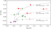 |
Fig. 6 Abundance ratios in r- II (circles), r- I (triangles) stars, and sample stars with normal [Eu/Fe] < −0.3 (squares). Smaller symbols represent stars with [Fe/H] > −2.5. An x symbol indicates a pure r-process ratio derived from average abundances in r- II sample stars. Different lines show abundance ratios calculated for mixtures of r-process and s-process with varying [Sr/Ba]earlyS. See the legend for designations. |
4.2 Literature data on Ba isotope measurements
4.2.1 Data on individual sample stars
Applying the abundance comparison method in 1D NLTE for HD 122563, Mashonkina et al. (2008) found Fodd = 0.22 ± 0.15, which agrees with our measurement of Fodd = ![$\[0.14_{-0.04}^{+0.09}\]$](/articles/aa/full_html/2025/07/aa55073-25/aa55073-25-eq17.png) . A slightly higher value of Fodd = 0.39 ± 0.06 was obtained by Mashonkina & Belyaev (2019) when using modified stellar atmosphere parameters of HD 122563 and an updated Ba II model atom. Using the profile fitting method in 1D LTE, Gallagher et al. (2012) found a non-physical result, yielding a negative Fodd = −0.12 ± 0.07 in HD 122563.
. A slightly higher value of Fodd = 0.39 ± 0.06 was obtained by Mashonkina & Belyaev (2019) when using modified stellar atmosphere parameters of HD 122563 and an updated Ba II model atom. Using the profile fitting method in 1D LTE, Gallagher et al. (2012) found a non-physical result, yielding a negative Fodd = −0.12 ± 0.07 in HD 122563.
For HD 4306, Cescutti et al. (2021) found a good agreement between the observed spectra and 1D LTE synthetic spectra of the Ba II resonance lines when assuming a pure s-process Ba isotope ratio.
For the r-process enhanced r- I star HD 108317, Mashonkina & Belyaev (2019) found consistent within 0.05 dex NLTE abundances from the resonance and subordinate lines of Ba II when using Fodd = 0.46. Our measurement of Fodd = ![$\[0.46_{-0.15}^{+0.24}\]$](/articles/aa/full_html/2025/07/aa55073-25/aa55073-25-eq18.png) is in agreement with Mashonkina & Belyaev (2019).
is in agreement with Mashonkina & Belyaev (2019).
For the strongly r-process enhanced r- II star HE2327–5642, Mashonkina et al. (2010) found a pure r-process Ba isotope ratio in line with our findings.
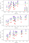 |
Fig. 7 Abundance difference between the subordinate and the resonance lines for different r- and s-process fractions (see the legend for designations). The arrows indicate the stars with weak lines of Eu II with EW < 6 mÅ. |
4.2.2 Data on MP stars derived from the abundance comparison method
Mashonkina & Zhao (2006, hereafter MZ06) determined NLTE abundances of Eu and Ba, using the r-process and solar Ba isotope mixture for a sample of MW stars. We combined these measurements with Sr NLTE abundance determinations for the same stars presented by Mashonkina et al. (2007). In total, we found 24 MP thick disc and halo dwarfs with Sr, Ba, and Eu abundances along with Ba isotope ratio determinations. The original publications of MZ06 and Mashonkina et al. (2007) do not include abundances from individual Ba II lines. However, we retrieved them from surviving handwritten notes and digitised the data, as presented in Table A.1 in the Appendix.
The majority of the selected MZ06 stars have metallicities in the range −1.4 < [Fe/H] <−0.3, with the two stars at [Fe/H] = −2.1. The MZ06 sample traces more advanced galactic chemical evolution stages compared to those in the present study and is affected by the main s-process in low- to intermediate-mass AGB stars producing Sr and Ba. However, regardless of the source of Sr and Ba in the MZ06 subsample, the data align well with our findings in the ΔBa − [Ba/Eu] and ΔBa−[Sr/Eu] diagrams (Fig. 8).
Jablonka et al. (2015) reports a Ba isotope ratio close to the s-process in two VMP stars in Sculptor dSph. These stars exhibit [Sr/Ba] ratios of 0.35 (ET0381) and −0.02 (Scl03059), both higher than the r-process value [Sr/Ba]r = −0.31. This finding supports our hypothesis regarding the synthesis of additional Sr via the early s-process.
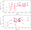 |
Fig. 8 Abundance difference between the subordinate and the resonance lines for pure r-process (circles) and solar Ba isotope mixture (squares) in our sample stars (filled symbols) and data from MZ06 (open symbols). For comparison with MZ06, we plot our ΔBa (sub.-res.) computed with the r-process Ba isotope mixture from Arlandini et al. (1999). |
4.3 [Sr/Ba] ratio in the early s-process
We aim to determine the chemical properties of the early s-process by subtracting the contribution of the main r-process from the Sr, Ba, and Eu abundances of the sample stars. Here, we assume that the main r-process and the early s-process are the two major sources of n-capture elements in the early Galaxy. Potential additional sources of n-capture elements are discussed in the following section.
The key point is that Sr and Ba originate from both the main r-process and the early s-process, while Eu is exclusively produced by the main r-process. This fact enables using Eu as a reference element. To estimate the [Sr/Ba]earlyS ratio produced by the early s-process, we use the following data: the [Sr/Eu] and [Ba/Eu] ratios in the sample stars; the pure r-process abundance ratios from the r- II sample stars: [Sr/Eu]r = −1.1, [Ba/Eu]r = −0.8, and [Sr/Ba]r = −0.3; solar abundances, log ε(Sr)⊙ = 2.88, log ε(Ba)⊙ = 2.17, log ε(Eu)⊙ = 0.51 from Lodders (2021).
In a given star, we can compute the number of Sr particles relative to the number of Eu particles. For example, in the Sun, this value amounts to N(Sr)/N(Eu) = 224. In r- II stars, the corresponding ratio is N(Sr)/N(Eu) = 18. Now let us compute the ratio in a given Sr-enhanced VMP star with [Sr/Eu] = 0.1, [Sr/Ba] = 0.7, and [Ba/Eu] = −0.6. In this star, [Sr/Eu] = 0.1 corresponds to log N(Sr)/N(Eu) = [Sr/Eu] + log N(Sr)/N(Eu)⊙ = 2.45, or N(Sr)/N(Eu) = 282. In other words, 18 Sr particles originate from the main r-process, while the remaining 264 Sr particles originate from the early s-process. Applying the same reasoning to the number of Ba particles, we find N(Ba)/N(Eu) = 7 for the pure r-process material and N(Ba)/N(Eu) = 11 in the example star. In this star, 7 Ba particles are produced by the main r-process, while the remaining 4 Ba particles originate from the early s-process. Combining our results for Sr and Ba in the star, we find that, in the early s-process, N(Sr)/N(Ba) = 264/4, or [Sr/Ba] = log (264/4) − log (N(Sr)/N(Ba))⊙ = 1.1.
Thus, we find that the example star with [Sr/Ba] = 0.7 can be represented as a mixture of main r-process material with [Sr/Ba]r = −0.3 and early s-process material with [Sr/Ba]earlyS = 1.1. From these values, we determine that in the example star, the main r-process and the early s-process are mixed in proportions of 75% and 25%, respectively.
Now, let us formalise this reasoning and define the procedure for estimating [Sr/Ba]earlyS. In a given star, its Sr, Ba, and Eu abundances can be represented as a mixture of r-process and early s-process material combined in a proportion kmix = Nr/NearlyS, where Nr and NearlyS denote the total number of particles produced by the r-process and the early s-process, respectively. Let us define N(Sr)earlyS/N(Ba)earlyS as XearlyS and express the number of Sr, Ba, and Eu particles in a given star relative to N(Ba)earlyS with
![$\[\begin{aligned}& \mathrm{N}(\mathrm{Sr})_*=\mathrm{X}_{\text {earlyS }}+\mathrm{k}_{\text {mix }} \cdot \mathrm{N}(\mathrm{Sr})_{\mathrm{r}} / \mathrm{N}(\mathrm{Ba})_{\mathrm{r}} \\& \mathrm{N}(\mathrm{Ba})_*=1+\mathrm{k}_{\text {mix }} \\& \mathrm{N}(\mathrm{Eu})_*=\mathrm{k}_{\text {mix}} \cdot \mathrm{N}(\mathrm{Eu})_{\mathrm{r}} / \mathrm{N}(\mathrm{Ba})_{\mathrm{r}}.\end{aligned}\]$](/articles/aa/full_html/2025/07/aa55073-25/aa55073-25-eq19.png)
Using the measured abundance ratios in a given star, we deduce:
![$\[\begin{aligned}& k_\mathrm{mix}=\left(\frac{{\mathrm{N}}({\mathrm{B a}})_* / {\mathrm{N}}({\mathrm{E u}})_*}{{\mathrm{N}}({\mathrm{B a}})_{\mathrm{r}} / {\mathrm{N}}({\mathrm{E u}})_{\mathrm{r}}}-1\right)^{-1} \\& X_{\text {earlyS}}=k_\mathrm{mix} \cdot\left(\frac{{\mathrm{N}}({\mathrm{S r}})_* / {\mathrm{N}}({\mathrm{E u}})_*}{{\mathrm{N}}({\mathrm{B a}})_{\mathrm{r}} / {\mathrm{N}}({\mathrm{E u}})_{\mathrm{r}}}-{\mathrm{N}}({\mathrm{S r}})_{\mathrm{r}} / {\mathrm{N}}({\mathrm{B a}})_{\mathrm{r}}\right)\end{aligned}\]$](/articles/aa/full_html/2025/07/aa55073-25/aa55073-25-eq20.png)
and finally, [Sr/Ba]earlyS = log XearlyS − (log ε(Sr)⊙ − log ε(Ba)⊙).
To evaluate the effectiveness of [Sr/Ba]earlyS synthesis in the early s-process, we selected sample stars with a significant contribution from this process – those with [Sr/Ba] > 0.1. From seven stars with −0.79 < [Ba/Eu] < − 0.36 and 0.13 < [Sr/Ba] < 0.74, we found an average [Sr/Ba]earlyS = 1.02 ± 0.24. When excluding two stars with weak Eu lines, we obtained [Sr/Ba]earlyS = 1.08 ± 0.17.
The selected seven stars exhibit different n-capture element abundance ratios; however, they consistently yield high [Sr/Ba]earlyS values. For example, CES1732+2344, with [Sr/Ba] = 0.13 and [Ba/Eu] = −0.79, and CES 1402+0941, with [Sr/Ba] = 0.74 and [Ba/Eu] = −0.55, provide close [Sr/Ba]earlyS values of 1.3 and 1.1, respectively. We attribute the variations in n-capture element abundance ratios among these stars to differing relative contributions of the r-process and the early s-process to their chemical composition. For the two stars mentioned above, we estimate that r-process and early s-process material are mixed in the following proportions: 95%/5% in CES1732+2344 and 55%/45% in CES1402+0941.
The remaining sample stars are either r- I or r- II type stars, dominated by the r-process. An exception is the most metal-rich sample star, CES1436–2906, with [Fe/H] = −2.15. Its chemical composition can be explained by a mixture of r-process and the main s-process, which produces [Sr/Ba] = 0 (Fig. 6).
For stars with moderate [Sr/Ba] enhancement, we found that the additional source of Sr synthesis is characterised by [Sr/Ba]earlyS = 0.5 (Fig. 6). This can be explained either by the main s-process contribution in addition to the early s-process or by variations in the effectiveness of Sr synthesis in the early s-process. The latter explanation seems more plausible, as the above stars have metallicities in the range −3 < [Fe/H] < −2.8, where the first intermediate-mass stars did not evolve yet to an AGB stage and the contribution of the main s-process is unlikely. Variations in the effectiveness of Sr synthesis in the early s-process are supported by different [Sr/Ba] enhancement observed in different systems: stars in ultra-faint dwarf galaxies exhibit systematically lower [Sr/Ba] ratios compared to those found in classical dSphs (Mashonkina et al. 2017b; Ji et al. 2019; Reichert et al. 2020; Sitnova et al. 2021).
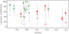 |
Fig. 9 R-process contribution to the 13 sample stars (excluding the three r- II stars) derived from the abundance ratios method (filled symbols) and Ba isotopes method (open symbols) as a function of [Sr/Eu]. Designations are the same as in Fig. 6. |
4.4 Potential sources of Sr and Ba synthesis beyond the main r-process and early s-process
When estimating [Sr/Ba]earlyS, we assume that the main r-process and the early s-process are the two primary n-capture element sources in the early Galaxy. However, we must consider the potential contribution of the i-process from massive stars (Banerjee et al. 2018) and weak r-process (Izutani et al. 2009) to the chemical composition of the sample stars. We do not consider a potential contribution from the νp process (Ghosh et al. 2022), as its nucleosynthesis yields for Sr and Ba are not available.
Similar to the r-process, the i-process follows a nucleosynthesis path through neutron-rich nuclei, followed by beta decay. Consequently, similar to the r-process, the i-process encounters the stable r-only isotopes 134Xe and 136Xe, which block the β-decay path and prevent the formation of 134Ba and 136Ba. As a result, the i-process is expected to effectively produce odd Ba isotopes 135Ba and 137Ba. For low-mass VMP AGB stars where the i-process occurs in their interiors, Choplin et al. (2021) found that 137Ba is surprisingly more abundant than 138Ba, which dominates in the solar system, as well as in the main s-process and r-process (Arlandini et al. 1999; Bisterzo et al. 2014). In other words, in terms of Ba isotopes, the contribution from the i-process appears similar to that of the r-process, increasing the fraction of odd Ba isotopes.
The r-process contribution to the chemical composition of a given star can be determined through element abundance ratios, as described above, along with another method based on Ba isotope analysis and achieving consistent abundances from the resonance and subordinate lines. For 13 sample stars, excluding the three r- II type stars, we computed the corresponding r-process fractions that result in ΔBa (sub.-res.) = 0. Figure 9 presents a comparison of r-process contributions derived from the two methods. Both methods yield results consistent within the error bars, though the uncertainties are sometimes uncomfortably large. If there were a significant contribution from the i-process, it would appear as a higher r-process contribution derived from the Ba isotope method compared to that from the element abundance ratio method, which is not observed in our data. The consistency of the two methods supports our hypothesis that, within our detection limits, the r-process and the early s-process are the two major Ba sources in the early Galaxy.
Regarding Sr synthesis, we demonstrated that, in addition to the main r-process, it is synthesised in the early s-process alongside the Ba even isotopes. However, the weak r-process may also produce a certain amount of Sr (Izutani et al. 2009). How can we identify a possible contribution to Sr abundance from the weak r-process in our sample stars? Let us take another look at Fig. 6. When excluding stars with [Fe/H] > −2.5, which may be contaminated by contribution from the main s-process, and r- II type stars, one can note that the remaining stars can be splitted into two groups according to their predicted [Sr/Ba] earlys: five stars (CES0419–3651, CES0338–2402, CES0215–2554, CES1222+1136, and CES1427–2214) predict [Sr/Ba]earlyS ≃ 0.5, while other five stars (CES1322–1355, CES1402+0941, CES1732+2344, CES0045–0932, CES2232–4138) predict [Sr/Ba]earlyS ≃ 1.0 (see Fig. 6, the dashed and solid line, respectively.) Let us assume that the higher predicted [Sr/Ba]earlyS can be interpreted as significant contamination by Sr produced in the weak r-process in addition to that Sr produced in the early s-process. Therefore, stars from the first group could be considered as having lower (or negligible) contribution from the weak r-process compared to stars from the second group.
Now let us examine the weak r-process yields available in Izutani et al. (2009). To trace the contribution of the weak r-process, one would need an element produced exclusively by that process. Sr, Y, and Zr are not suitable for distinguishing between contributions from the weak r-process and the early s-process. Figure 12 in Izutani et al. (2009) demonstrates that the weak r-process produces Zn as efficiently as Sr, Y, and Zr. In contrast, the s-process in VMP massive rotating stars produces a negligible amount of Zn (see Fig. 29 in Limongi & Chieffi 2018). Therefore, we select Zn as a tracer of the weak r-process. Following our hypothesis regarding the different contributions of the weak r-process to stars in the first and second groups, we might expect them to exhibit distinct Zn abundances, with higher values in the second group stars. Using the Zn abundances determined in LB22, we computed the average [Zn/Fe] = 0.27 ± 0.08 for the first group and 0.30 ± 0.12 for the second group. Therefore, we found no significant difference in [Zn/Fe] ratios between the two groups. In both groups, the stars span the same metallicity range, with [Fe/H] from −2.9 to −2.5, and we found no systematic difference in the other chemical element abundances between the two groups. Based on our results, we found no strong evidence supporting a contribution from the weak r-process to the chemical composition of our sample stars.
4.5 Comparison with chemical evolution model predictions
We employed a stochastic chemical evolution model of the Galactic halo, making use of the GEMS code described in Rizzuti et al. (2025) and based on the stochastic models of Cescutti (2008) and Rizzuti et al. (2021). The model traces the early evolutionary stages within the first 1 Gyr of the halo formation, with a timestep of 1 Myr. Stochasticity is introduced by dividing the halo into 10 000 cubic regions, each considered isolated and containing the typical mass of gas swept by a SN-II explosion. Within each region, star formation, gas inflow and outflow are modelled, and gas recycling occurs at each step due to enrichment from evolving stars of different masses.
In the model, we included three sources of n-capture element synthesis: the main r-process, the s-process in rotating massive stars, and the s-process in AGB stars; however, the latter only contributes to the chemical evolution at [Fe/H] > −2. We assumed that the main r-process occurs in merging neutron stars with progenitor masses of 9–50 M⊙. A binary fraction of 0.018 and a fixed coalescence time-scale of 1 Myr are adopted according to Matteucci et al. (2014) and Cescutti et al. (2015). We employed the empirical r-process ratios [Sr/Ba]r = −0.3 and [Ba/Eu]r = −0.8 for consistency with this study. The outcome of our chemical evolution results would not change significantly if magneto-rotational SNe are adopted as producers of r-process, instead of merging neutron stars with a very short delay. For the s-process in rotating massive stars (13–120 M⊙), we used yields from the Limongi & Chieffi (2018) grid, ejected through stellar winds and explosions. For the main s-process in AGB stars, we used the yields from the FRUITY database (Cristallo et al. 2011). Iron yields were taken from Limongi & Chieffi (2018). For more details on the code, see Rizzuti et al. (2025).
Figure 10 compares the [Sr/Ba] and [Ba/Eu] ratios derived for our sample stars with the simulated data for long-living stars in the chemical evolution model. For consistency, we extracted model data for stars with metallicities in the range −3.1 < [Fe/H] < −2.1, matching our sample. The derived abundance ratios generally agree with model predictions. However, reproducing the highest observed [Sr/Ba] values requires a slightly higher predicted [Sr/Ba], which could be achieved by assuming slower rotation velocities in massive stars with −3.1 < [Fe/H] < −2.1.
Figure 11 compares the derived fraction of odd Ba isotopes as a function of [Sr/Ba] with chemical evolution model predictions. The observed values span a wide range, with Fodd varying from pure s-process to pure r-process values. Notably, the model predicts a significant number of stars with [Sr/Ba] < −0.3, originating from material produced by massive VMP stars with the highest rotational velocities, as faster rotation leads to lower [Sr/Ba] production. Although our sample does not include stars enriched by such objects, we note that VMP stars with [Sr/Ba] < −0.3 should exhibit a low Fodd < 0.2. Determining Ba isotopic fractions in such stars would provide key constraints on the rotational velocities of massive VMP stars.
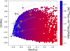 |
Fig. 10 Comparison of the derived abundance ratios with the simulated data for long-living stars in the chemical evolution model. Designations are the same as in Fig. 6. Colour bar indicates the predicted fraction of odd Ba isotopes. |
4.6 Other light n-capture elements: Y and Zr
We employ Sr as a tracer of light n-capture elements sources, although Y and Zr are also recognised as light n-capture elements and exhibit similar behaviour in VMP stars. Our conclusion regarding the joint synthesis of Sr and the even Ba isotopes can also be extended to Y and Zr. Figure 12 shows Fodd as a function of [Sr/Ba], [Y/Ba], and [Zr/Ba], with Y and Zr abundances taken from LB22. All three elements display a similar trend: Fodd decreases with increasing [X/Ba], supporting the idea of co-production of Sr, Y, and Zr alongside the even Ba isotopes.
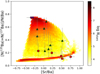 |
Fig. 11 Comparison of the derived fraction of odd Ba isotopes with the simulated data for long-living stars in the chemical evolution model. Designations are the same as in Fig. 6. Colour bar indicates the predicted number of stars in each area of the diagram. |
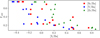 |
Fig. 12 Fodd as a function of [X/Ba] (see legend) in the sample stars. |
5 Conclusions
We presented a spectroscopic analysis of 16 VMP stars and determined their Sr, Ba, and Eu NLTE abundances, along with the contributions of the r- and s-processes to their Ba isotope mixture. For Ba isotope ratio analysis, we employed a method based on abundance comparisons between the resonance and subordinate lines of Ba II. This method is most effective within a specific stellar atmosphere and barium abundance range, where the EWs of the Ba II resonance lines range from 60 to 130 mÅ, making them sensitive to the Ba isotope ratio while avoiding excessive saturation.
Our results provide observational constraints on the source of Sr operating at the early epoch of Galactic chemical evolution. Our findings are summarised as follows:
- ◦
We find a higher s-process contribution to Ba isotopes in stars with greater [Sr/Eu] ratio, suggesting that the additional Sr synthesis was due to the early s-process occurring in massive stars. Our finding matches the Galactic chemical evolution model predictions of Cescutti et al. (2013), Cescutti & Chiappini (2014), and Rizzuti et al. (2021).
- ◦
The early s-process produces not only Sr but also Ba; therefore it is not a weak s-process. The most likely candidate for the early s-process is a non-standard s-process occurring in massive stars (Frischknecht et al. 2012, 2016; Choplin et al. 2018; Limongi & Chieffi 2018).
- ◦
Using Sr-enhanced stars, we estimate that the [Sr/Ba] ratio produced by the early s-process could be as high as [Sr/Ba]earlyS = 1.1 ± 0.2. Regarding the potential synthesis of Sr and Ba in the i-process in massive stars, our results for Ba isotopes and element abundances argue that there was no detectable contribution from this process within the error bars in our sample stars.
Data availability
The full Tables 2, 3, and 4 are available at the CDS https://cdsarc.cds.unistra.fr/viz-bin/cat/J/A+A/699/A262
Acknowledgements
The authors thank the referee for carefully reading the manuscript and providing valuable feedback. We acknowledge A. Alencastro Puls for reading the manuscript and providing feedback. TS is grateful to Yu. V. Pakhomov for providing his code for echelle orders merging. LL and CJH acknowledge the support by the State of Hesse within the Research Cluster ELEMENTS (Project ID 500/10.006). FR is a fellow of the Alexander von Humboldt Foundation. FR acknowledges support by the Klaus Tschira Foundation. FR and GC acknowledge the National Recovery and Resilience Plan (NRRP), Mission 4, Component 2, Investment 1.1, Call for tender No. 104 published on 2.2.2022 by the Italian Ministry of University and Research (MUR), funded by the European Union – NextGenerationEU – Project ‘Cosmic POT’ (PI: L. Magrini) Grant No. 2022X4TM3H by the MUR. GC thanks for the support INAF (Large Grant 2023, EPOCH and the MiniGrant 2022 Checs). GC and CJH acknowledge the European Union (ChETEC-INFRA, project no. 101008324). CJH acknowledges HFHF. PB acknowledges support from the ERC advanced grant N. 835087 – SPIAKID. This study has made use of the Keck Observatory Archive, which is operated by the W. M. Keck Observatory and the NASA Exoplanet Science Institute, under contract with the National Aeronautics and Space Administration.
Appendix A Additional table
Stellar parameters and abundances from individual lines of Sr II, Ba II, and Eu II from MZ06 and Mashonkina et al. (2007).
References
- Aoki, W., Honda, S., Beers, T. C., et al. 2005, ApJ, 632, 611 [Google Scholar]
- Arcones, A., & Bliss, J. 2014, J. Phys. G Nuclear Phys., 41, 044005 [Google Scholar]
- Arlandini, C., Käppeler, F., Wisshak, K., et al. 1999, ApJ, 525, 886 [Google Scholar]
- Banerjee, P., Qian, Y.-Z., & Heger, A. 2018, ApJ, 865, 120 [Google Scholar]
- Barklem, P. S., Christlieb, N., Beers, T. C., et al. 2005, A&A, 439, 129 [NASA ADS] [CrossRef] [EDP Sciences] [Google Scholar]
- Bergemann, M. 2011, MNRAS, 413, 2184 [NASA ADS] [CrossRef] [Google Scholar]
- Bisterzo, S., Travaglio, C., Gallino, R., Wiescher, M., & Käppeler, F. 2014, ApJ, 787, 10 [NASA ADS] [CrossRef] [Google Scholar]
- Butler, K. 1984, Ph.D. Thesis, University of London, UK [Google Scholar]
- Cescutti, G. 2008, A&A, 481, 691 [NASA ADS] [CrossRef] [EDP Sciences] [Google Scholar]
- Cescutti, G., & Chiappini, C. 2014, A&A, 565, A51 [NASA ADS] [CrossRef] [EDP Sciences] [Google Scholar]
- Cescutti, G., Chiappini, C., Hirschi, R., Meynet, G., & Frischknecht, U. 2013, A&A, 553, A51 [NASA ADS] [CrossRef] [EDP Sciences] [Google Scholar]
- Cescutti, G., Romano, D., Matteucci, F., Chiappini, C., & Hirschi, R. 2015, A&A, 577, A139 [NASA ADS] [CrossRef] [EDP Sciences] [Google Scholar]
- Cescutti, G., Morossi, C., Franchini, M., et al. 2021, A&A, 654, A164 [NASA ADS] [CrossRef] [EDP Sciences] [Google Scholar]
- Chiappini, C., Frischknecht, U., Meynet, G., et al. 2011, Nature, 472, 454 [Google Scholar]
- Choplin, A., Hirschi, R., Meynet, G., et al. 2018, A&A, 618, A133 [NASA ADS] [CrossRef] [EDP Sciences] [Google Scholar]
- Choplin, A., Siess, L., & Goriely, S. 2021, A&A, 648, A119 [NASA ADS] [CrossRef] [EDP Sciences] [Google Scholar]
- Choplin, A., Siess, L., Goriely, S., & Martinet, S. 2024, A&A, 684, A206 [NASA ADS] [CrossRef] [EDP Sciences] [Google Scholar]
- Christlieb, N., Beers, T. C., Barklem, P. S., et al. 2004, A&A, 428, 1027 [NASA ADS] [CrossRef] [EDP Sciences] [Google Scholar]
- Collet, R., Asplund, M., & Nissen, P. E. 2009, PASA, 26, 330 [NASA ADS] [CrossRef] [Google Scholar]
- Cowan, J. J., & Rose, W. K. 1977, ApJ, 212, 149 [Google Scholar]
- Cowley, C. R., & Frey, M. 1989, ApJ, 346, 1030 [Google Scholar]
- Cristallo, S., Piersanti, L., Straniero, O., et al. 2011, ApJS, 197, 17 [NASA ADS] [CrossRef] [Google Scholar]
- Eichler, M., Nakamura, K., Takiwaki, T., et al. 2018, J. Phys. G Nucl. Phys., 45, 014001 [NASA ADS] [CrossRef] [Google Scholar]
- Fernandes de Melo, R., Lombardo, L., Alencastro Puls, A., et al. 2024, A&A, 691, A220 [NASA ADS] [CrossRef] [EDP Sciences] [Google Scholar]
- François, P., Depagne, E., Hill, V., et al. 2007, A&A, 476, 935 [Google Scholar]
- Frischknecht, U., Hirschi, R., & Thielemann, F. K. 2012, A&A, 538, L2 [NASA ADS] [CrossRef] [EDP Sciences] [Google Scholar]
- Frischknecht, U., Hirschi, R., Pignatari, M., et al. 2016, MNRAS, 456, 1803 [Google Scholar]
- Fröhlich, C., Martínez-Pinedo, G., Liebendörfer, M., et al. 2006, Phys. Rev. Lett., 96, 142502 [CrossRef] [Google Scholar]
- Gaia Collaboration (Brown, A. G. A., et al.) 2021, A&A, 649, A1 [NASA ADS] [CrossRef] [EDP Sciences] [Google Scholar]
- Gallagher, A. J., Ryan, S. G., García Pérez, A. E., & Aoki, W. 2010, A&A, 523, A24 [NASA ADS] [CrossRef] [EDP Sciences] [Google Scholar]
- Gallagher, A. J., Ryan, S. G., Hosford, A., et al. 2012, A&A, 538, A118 [NASA ADS] [CrossRef] [EDP Sciences] [Google Scholar]
- Gallagher, A. J., Ludwig, H. G., Ryan, S. G., & Aoki, W. 2015, A&A, 579, A94 [NASA ADS] [CrossRef] [EDP Sciences] [Google Scholar]
- Ghosh, S., Wolfe, N., & Fröhlich, C. 2022, ApJ, 929, 43 [NASA ADS] [CrossRef] [Google Scholar]
- Giddings, J. 1981, Ph.D. Thesis, University of London, UK [Google Scholar]
- Gratton, R. G., & Sneden, C. 1994, A&A, 287, 927 [NASA ADS] [Google Scholar]
- Gustafsson, B., Edvardsson, B., Eriksson, K., et al. 2008, A&A, 486, 951 [NASA ADS] [CrossRef] [EDP Sciences] [Google Scholar]
- Hansen, C. J., Primas, F., Hartman, H., et al. 2012, A&A, 545, A31 [NASA ADS] [CrossRef] [EDP Sciences] [Google Scholar]
- Hansen, C. J., Montes, F., & Arcones, A. 2014, ApJ, 797, 123 [NASA ADS] [CrossRef] [Google Scholar]
- Hayek, W., Wiesendahl, U., Christlieb, N., et al. 2009, A&A, 504, 511 [NASA ADS] [CrossRef] [EDP Sciences] [Google Scholar]
- Izutani, N., Umeda, H., & Tominaga, N. 2009, ApJ, 692, 1517 [Google Scholar]
- Jablonka, P., North, P., Mashonkina, L., et al. 2015, A&A, 583, A67 [NASA ADS] [CrossRef] [EDP Sciences] [Google Scholar]
- Ji, A. P., Simon, J. D., Frebel, A., Venn, K. A., & Hansen, T. T. 2019, ApJ, 870, 83 [NASA ADS] [CrossRef] [Google Scholar]
- Käppeler, F., Gallino, R., Bisterzo, S., & Aoki, W. 2011, Rev. Mod. Phys., 83, 157 [Google Scholar]
- Kobayashi, C., Karakas, A. I., & Lugaro, M. 2020, ApJ, 900, 179 [Google Scholar]
- Kochukhov, O. 2018, Astrophysics Source Code Library [record ascl:1805.015] [Google Scholar]
- Kurucz, R. L. 2005, Mem. Soc. Astron. Ital. Suppl., 8, 14 [Google Scholar]
- Lambert, D. L., & Allende Prieto, C. 2002, MNRAS, 335, 325 [Google Scholar]
- Limongi, M., & Chieffi, A. 2018, ApJS, 237, 13 [NASA ADS] [CrossRef] [Google Scholar]
- Lodders, K. 2021, Space Sci. Rev., 217, 44 [NASA ADS] [CrossRef] [Google Scholar]
- Lombardo, L., Bonifacio, P., François, P., et al. 2022, A&A, 665, A10 [NASA ADS] [CrossRef] [EDP Sciences] [Google Scholar]
- Lombardo, L., Hansen, C. J., Rizzuti, F., et al. 2025, A&A, 693, A293 [NASA ADS] [CrossRef] [EDP Sciences] [Google Scholar]
- Magain, P. 1995, A&A, 297, 686 [NASA ADS] [Google Scholar]
- Magain, P., & Zhao, G. 1993, A&A, 268, L27 [NASA ADS] [Google Scholar]
- Mallinson, J. W. E., Lind, K., Amarsi, A. M., et al. 2022, A&A, 668, A103 [NASA ADS] [CrossRef] [EDP Sciences] [Google Scholar]
- Mashonkina, L. I., & Belyaev, A. K. 2019, Astron. Lett., 45, 341 [NASA ADS] [CrossRef] [Google Scholar]
- Mashonkina, L., & Christlieb, N. 2014, A&A, 565, A123 [NASA ADS] [CrossRef] [EDP Sciences] [Google Scholar]
- Mashonkina, L., & Gehren, T. 2000, A&A, 364, 249 [NASA ADS] [Google Scholar]
- Mashonkina, L., & Gehren, T. 2001, A&A, 376, 232 [CrossRef] [EDP Sciences] [Google Scholar]
- Mashonkina, L., & Zhao, G. 2006, A&A, 456, 313 [NASA ADS] [CrossRef] [EDP Sciences] [Google Scholar]
- Mashonkina, L. I., Vinogradova, A. B., Ptitsyn, D. A., Khokhlova, V. S., & Chernetsova, T. A. 2007, Astron. Rep., 51, 903 [NASA ADS] [CrossRef] [Google Scholar]
- Mashonkina, L., Zhao, G., Gehren, T., et al. 2008, A&A, 478, 529 [NASA ADS] [CrossRef] [EDP Sciences] [Google Scholar]
- Mashonkina, L., Christlieb, N., Barklem, P. S., et al. 2010, A&A, 516, A46 [NASA ADS] [CrossRef] [EDP Sciences] [Google Scholar]
- Mashonkina, L., Gehren, T., Shi, J.-R., Korn, A. J., & Grupp, F. 2011, A&A, 528, A87 [NASA ADS] [CrossRef] [EDP Sciences] [Google Scholar]
- Mashonkina, L., Jablonka, P., Pakhomov, Y., Sitnova, T., & North, P. 2017a, A&A, 604, A129 [NASA ADS] [CrossRef] [EDP Sciences] [Google Scholar]
- Mashonkina, L., Jablonka, P., Sitnova, T., Pakhomov, Y., & North, P. 2017b, A&A, 608, A89 [NASA ADS] [CrossRef] [EDP Sciences] [Google Scholar]
- Mashonkina, L., Pakhomov, Y. V., Sitnova, T., et al. 2022, MNRAS, 509, 3626 [Google Scholar]
- Mashonkina, L., Pakhomov, Y., Sitnova, T., et al. 2023, MNRAS, 524, 3526 [Google Scholar]
- Matteucci, F., Romano, D., Arcones, A., Korobkin, O., & Rosswog, S. 2014, MNRAS, 438, 2177 [Google Scholar]
- McWilliam, A., Preston, G. W., Sneden, C., & Searle, L. 1995, AJ, 109, 2757 [Google Scholar]
- Pakhomov, Y. V., Ryabchikova, T. A., & Piskunov, N. E. 2019, Astron. Rep., 63, 1010 [NASA ADS] [CrossRef] [Google Scholar]
- Pignatari, M., Gallino, R., Meynet, G., et al. 2008, ApJ, 687, L95 [Google Scholar]
- Prantzos, N., Abia, C., Cristallo, S., Limongi, M., & Chieffi, A. 2020, MNRAS, 491, 1832 [Google Scholar]
- Qian, Y. Z., & Wasserburg, G. J. 2007, Phys. Rep., 442, 237 [Google Scholar]
- Raiteri, C. M., Busso, M., Gallino, R., & Picchio, G. 1991a, ApJ, 371, 665 [Google Scholar]
- Raiteri, C. M., Busso, M., Gallino, R., Picchio, G., & Pulone, L. 1991b, ApJ, 367, 228 [Google Scholar]
- Reichert, M., Hansen, C. J., Hanke, M., et al. 2020, A&A, 641, A127 [NASA ADS] [CrossRef] [EDP Sciences] [Google Scholar]
- Rizzuti, F., Cescutti, G., Matteucci, F., et al. 2021, MNRAS, 502, 2495 [NASA ADS] [CrossRef] [Google Scholar]
- Rizzuti, F., Cescutti, G., Molaro, P., et al. 2025, A&A, 698, A118 [Google Scholar]
- Roederer, I. U. 2013, AJ, 145, 26 [CrossRef] [Google Scholar]
- Roederer, I. U., Sakari, C. M., Placco, V. M., et al. 2018, ApJ, 865, 129 [NASA ADS] [CrossRef] [Google Scholar]
- Rolfs, C., Trautvetter, H. P., & Rodney, W. S. 1987, Rep. Progr. Phys., 50, 233 [Google Scholar]
- Ryabchikova, T., Piskunov, N., Kurucz, R. L., et al. 2015, Phys. Scr, 90, 054005 [Google Scholar]
- Shah, S. P., Ezzeddine, R., Roederer, I. U., et al. 2024, MNRAS, 529, 1917 [NASA ADS] [CrossRef] [Google Scholar]
- Simmerer, J., Sneden, C., Cowan, J. J., et al. 2004, ApJ, 617, 1091 [Google Scholar]
- Sitnova, T., Zhao, G., Mashonkina, L., et al. 2015, ApJ, 808, 148 [Google Scholar]
- Sitnova, T. M., Mashonkina, L. I., & Ryabchikova, T. A. 2016, MNRAS, 461, 1000 [Google Scholar]
- Sitnova, T. M., Yakovleva, S. A., Belyaev, A. K., & Mashonkina, L. I. 2020, Astron. Lett., 46, 120 [NASA ADS] [CrossRef] [Google Scholar]
- Sitnova, T. M., Mashonkina, L. I., Tatarnikov, A. M., et al. 2021, MNRAS, 504, 1183 [NASA ADS] [CrossRef] [Google Scholar]
- Sneden, C., Cowan, J. J., Lawler, J. E., et al. 2003, ApJ, 591, 936 [NASA ADS] [CrossRef] [Google Scholar]
- Sneden, C., Cowan, J. J., & Gallino, R. 2008, ARA&A, 46, 241 [Google Scholar]
- Spite, M., & Spite, F. 1978, A&A, 67, 23 [NASA ADS] [Google Scholar]
- Travaglio, C., Gallino, R., Arnone, E., et al. 2004, ApJ, 601, 864 [Google Scholar]
- Tsymbal, V., Ryabchikova, T., & Sitnova, T. 2019, in Astronomical Society of the Pacific Conference Series, 518, Physics of magnetic stars, eds. I. I. Romanyuk, I. A. Yakunin, & D. O. Kudryavtsev, 247 [Google Scholar]
- Wood, M. P., Lawler, J. E., Sneden, C., & Cowan, J. J. 2013, ApJS, 208, 27 [NASA ADS] [CrossRef] [Google Scholar]
- Woosley, S. E., & Hoffman, R. D. 1992, ApJ, 395, 202 [CrossRef] [Google Scholar]
Here, we employ the notation of Christlieb et al. (2004) for the r-process enhanced star classification.
All Tables
Stellar sample, atmospheric parameters, and characteristics of the observed spectra used for the Ba II 4554 Å line analysis.
NLTE abundance corrections and EWs in mÅ for Ti II lines as a function of Teff, log g, and [Fe/H].
NLTE and LTE abundances and EWs from individual Sr II and Eu II lines in the sample stars.
Stellar parameters and abundances from individual lines of Sr II, Ba II, and Eu II from MZ06 and Mashonkina et al. (2007).
All Figures
|
Fig. 1 Top panel: NLTE abundances from Ti II lines in CES1427–2214 as a function of the EW computed for ξt = 1.60 km s−1 (squares) and 1.85 km s−1 (circles). Bottom panel: NLTE abundances from Fe I (triangles) and Fe II (asterisks) lines in CES1427–2214 computed for ξt = 1.60 km s−1. |
| In the text | |
|
Fig. 2 Ba II 4934 Å line profile in the observed spectrum (circles) of the most metal-rich sample star CES1436–2906 with [Fe/H] = −2.15 along with a synthetic best-fit NLTE spectrum (solid line) and a spectrum, calculated neglecting the Fe I 4934 Å line (dashed line). |
| In the text | |
|
Fig. 3 Departure coefficients of the ground state of Ba II (6s) and the upper levels of the resonance transitions in a model atmosphere of a VMP giant. The vertical dashes indicate the line core formation depths of the resonance lines of different strength: 130 mÅ and 60 mÅ at logτ5000 = −2.1 and −1.2, respectively. |
| In the text | |
|
Fig. 4 NLTE abundances from the Ba II 4554 Å and 4934 Å lines as a function of r-process contribution to Ba isotopes in the two sample stars. The EWs of the resonance lines are indicated. |
| In the text | |
|
Fig. 5 Top panel: Ba II 4554 Å line profile in the observed spectrum (circles) of HE0336–2412 (CES0338–2402). Synthetic best-fit NLTE spectra, derived using pure r-process (dashed line) and pure s-process (dotted line) Ba isotope mixtures are almost indistinguishable, demonstrating that a reasonable fit can be achieved with any adopted isotope ratio. Vertical dashes show the relative contribution of different Ba isotopes to the r-process and s-process; see legend for designations. Bottom panel: Same as the top panel for HD 27928 (CES0422–3715). |
| In the text | |
|
Fig. 6 Abundance ratios in r- II (circles), r- I (triangles) stars, and sample stars with normal [Eu/Fe] < −0.3 (squares). Smaller symbols represent stars with [Fe/H] > −2.5. An x symbol indicates a pure r-process ratio derived from average abundances in r- II sample stars. Different lines show abundance ratios calculated for mixtures of r-process and s-process with varying [Sr/Ba]earlyS. See the legend for designations. |
| In the text | |
|
Fig. 7 Abundance difference between the subordinate and the resonance lines for different r- and s-process fractions (see the legend for designations). The arrows indicate the stars with weak lines of Eu II with EW < 6 mÅ. |
| In the text | |
|
Fig. 8 Abundance difference between the subordinate and the resonance lines for pure r-process (circles) and solar Ba isotope mixture (squares) in our sample stars (filled symbols) and data from MZ06 (open symbols). For comparison with MZ06, we plot our ΔBa (sub.-res.) computed with the r-process Ba isotope mixture from Arlandini et al. (1999). |
| In the text | |
|
Fig. 9 R-process contribution to the 13 sample stars (excluding the three r- II stars) derived from the abundance ratios method (filled symbols) and Ba isotopes method (open symbols) as a function of [Sr/Eu]. Designations are the same as in Fig. 6. |
| In the text | |
|
Fig. 10 Comparison of the derived abundance ratios with the simulated data for long-living stars in the chemical evolution model. Designations are the same as in Fig. 6. Colour bar indicates the predicted fraction of odd Ba isotopes. |
| In the text | |
|
Fig. 11 Comparison of the derived fraction of odd Ba isotopes with the simulated data for long-living stars in the chemical evolution model. Designations are the same as in Fig. 6. Colour bar indicates the predicted number of stars in each area of the diagram. |
| In the text | |
|
Fig. 12 Fodd as a function of [X/Ba] (see legend) in the sample stars. |
| In the text | |
Current usage metrics show cumulative count of Article Views (full-text article views including HTML views, PDF and ePub downloads, according to the available data) and Abstracts Views on Vision4Press platform.
Data correspond to usage on the plateform after 2015. The current usage metrics is available 48-96 hours after online publication and is updated daily on week days.
Initial download of the metrics may take a while.