| Issue |
A&A
Volume 699, July 2025
|
|
|---|---|---|
| Article Number | A189 | |
| Number of page(s) | 19 | |
| Section | Extragalactic astronomy | |
| DOI | https://doi.org/10.1051/0004-6361/202554434 | |
| Published online | 09 July 2025 | |
An improved Seyfert-low ionization nuclear emission-line region classification line in the [N II] BPT diagram
School of Physical Science and Technology, Guangxi University, No. 100, Daxue East Road, Nanning, 530004, P.R. China
⋆ Corresponding author: This email address is being protected from spambots. You need JavaScript enabled to view it.
Received:
9
March
2025
Accepted:
23
May
2025
Abstract
Context. In this paper, we propose an improved Seyfert-low ionization nuclear emission-line region (LINER) classification line (=S-L line) in the [N II] BPT diagram, based on a sample of 47 968 low-redshift, narrow-emission-line galaxies from SDSS DR16, motivated by different S-L lines reported in the [N II] BPT diagram through different methods. We first applied the method successfully applied in the [S II] and [O I] BPT diagrams, however, the method does not lead to an accepted S-L line in the [N II] BPT diagram. Meanwhile, the S-L lines previously proposed in the [N II] BPT diagram are different from each other.
Aims. We aim to check which proposed S-L line is better or to determine an improved one in the [N II] BPT diagram by a new method.
Methods. We visualized the Seyferts and LINERs that had already been classified in the [S II] and/or [O I] BPT diagrams in the [N II] BPT diagram. The intersection boundary between the two contour maps was then considered as the S-L line in the [N II] BPT diagram.
Results. Rather than the previously proposed S-L lines, the new S-L line can lead to more efficient and harmonious classifications of Seyferts and LINERs, especially in the composite galaxy region, in the [N II] BPT diagram. Furthermore, based on the discussed S-L lines, the number ratio of Type-2 Seyferts to Type-2 LINERs differs significantly from that of Type-1 Seyferts to Type-1 LINERs in the [N II] BPT diagram. This suggests that about 90% of Type-2 LINERs are non-active galactic nucleus (non-AGN)-related objects, true Type-2 AGNs, or objects that exhibit both Seyfert and LINER characteristics.
Key words: galaxies: active / galaxies: nuclei / quasars: emission lines / galaxies: Seyfert
© The Authors 2025
 Open Access article, published by EDP Sciences, under the terms of the Creative Commons Attribution License (https://creativecommons.org/licenses/by/4.0), which permits unrestricted use, distribution, and reproduction in any medium, provided the original work is properly cited.
This article is published in open access under the Subscribe to Open model. This email address is being protected from spambots. You need JavaScript enabled to view it. to support open access publication.
1. Introduction
The well-known BPT (Baldwin, Phillips & Terlevich) diagrams have been widely accepted for classifying narrow-emission-line galaxies, since Baldwin et al. (1981) and Veilleux & Osterbrock (1987) clearly showed that different types of extragalactic objects occupy in different regions in spaces of flux ratios of different narrow emission lines, especially flux ratios of [O III]λ5007 Å to Hβ versus [N II]λ6584 Å to Hα (the [N II] BPT diagram), of [O III]λ5007 Å to Hβ versus [S II]λ6717,6731 Å to Hα (the [S II] BPT diagram), and of [O III]λ5007 Å to Hβ versus [O I]λ6300 Å to Hα (the [O I] BPT diagram). In the 1980s, due to the small sample sizes of narrow-emission-line galaxies applied in the BPT diagrams (only about 140 narrow-emission-line galaxies are discussed in Baldwin et al. 1981, and about 240 narrow-emission-line galaxies are discussed in Veilleux & Osterbrock 1987), the classifications for different types of narrow-emission-line galaxies, such as Type-2 Seyferts and H II galaxies, were clear enough. However, with the very rapid growth in the number of detected narrow-emission-line galaxies, there are no apparent classification lines between different types of galaxies in the BPT diagrams. Therefore, how to give efficient classifications (or classification lines between different types of galaxies) in the BPT diagrams is a meaningful research subject.
Kewley et al. (2001) reported the clear theoretical classification lines (hereafter Ke01 lines) between H II regions and AGNs (active galactic nuclei) in the three BPT diagrams, after considering narrow-emission-line ratios theoretically determined by ionization photons generated by the PEGASE v2.0 and STARBURST99 codes. Kauffmann et al. (2003a) proposed an empirical classification line (hereafter the Ka03 line) in the [N II] BPT diagram through a large sample of 22 623 AGNs from the SDSS (Sloan Digital Sky Survey) that led to an efficient classification of composite galaxies. Stasińska et al. (2006) proposed a classification line, lower than the Ka03 line, between pure normal star-forming galaxies and AGNs in the [N II] BPT diagram, based on a sample of 20 000 galaxies from the SDSS. They considered photoionization models informed by synthetic stellar radiation and a broken power-law spectrum for AGNs. Kewley et al. (2006) proposed the widely accepted classification lines between Seyferts (commonly, Type-2 Seyferts) and LINERs (low ionization nuclear emission-line regions) in the [S II] and [O I] BPT diagrams based on a sample of 85 224 emission-line galaxies from the SDSS, but not in the [N II] BPT diagram. de Souza et al. (2017) applied Gaussian mixture models to discuss the classification lines between different types of narrow-emission-line galaxies in the [N II] BPT diagram. They effectively distinguished AGNs, composite galaxies, and H II regions, but struggled with Seyferts and LINERs due to overlap. Teimoorinia & Keown (2018) proposed that AGNs can be well distinguished from star-forming galaxies through a machine learning approach. Zhang et al. (2020) verify the classifications of AGNs and H II galaxies in the BPT diagrams based on the t-distributed Stochastic Neighbor Embedding technique applied to 35 857 local narrow-emission-line galaxies. Agostino et al. (2021, 2023a) improve the distinctions between AGNs and star-forming galaxies by truncating the lower portion of the Ka03 line with a straight line at log([N II]/Hα) = −0.35. A comprehensive review of emission-line-based classification methods can be found in Kewley et al. (2019).
At the current stage, there are clear classification lines between H II regions and AGNs in all the three BPT diagrams. However, Seyferts and LINERs are only well classified in the [S II] and [O I] BPT diagrams, since these two diagrams show two distinct branches above the Ke01 line. In contrast, the [N II] BPT diagram only shows one thick branch at the upper right side of the Ke01 line, because the [N II]/Hα ratio does not offer sufficient distinction between these two branches (Stasińska et al. 2006; Kewley et al. 2019). This distinction, as shown in our BPT diagrams in the following sections, leads to only Seyferts and LINERs with apparent [S II] and/or [O I] narrow forbidden emission lines being well classified. Considering that the number of galaxies with [N II] emission lines far exceeds that of those with [S II] or [O I] narrow emission lines, classifying Seyferts and LINERs in the [N II] BPT diagram will undoubtedly provide richer samples by including more galaxies with weak [S II] or [O I] but apparent [N II] emission lines, and facilitate the smooth exclusion of LINERs from Seyferts in future studies to test the unified model of AGNs. Therefore, it is useful to determine a classification line in the [N II] BPT diagram to effectively classify Seyferts and LINERs, since some LINERs are probably not AGN-related objects.
The concept of LINERs was first defined by Heckman (1980), and Ho et al. (1996) improved their definitions. However, there is still controversy about the physical mechanism of LINERs. To begin with, some LINERs are powered by black hole accretion systems, which indicates clear AGN-related activity. Agostino & Salim (2019) concluded that the proportion of LINERs with X-ray detection is similar to that of AGNs (Seyferts). Moreover, Agostino et al. (2023b) found that LINERs detected in X-rays are not significantly different from those undetected, which supports the idea that many LINERs are indeed genuine AGNs to some extent. In contrast, many researchers tend to believe that the dominant mechanism in some LINERs is non-AGN-related. Cid Fernandes et al. (2009) proposed that most LINER-like systems in the SDSS should not be included in any census of actively accreting black holes as they are consistent with being retired galaxies where ionizing photons are produced by aging stars. Singh et al. (2013) found that the radial emission-line surface brightness distribution of 48 galaxies with LINER-like emission, based on integral field spectroscopy data from the Calar Alto Legacy Integral Field Area survey, was inconsistent with ionization by a central point source (AGN illumination), which suggests that LINERs cannot be solely attributed to AGNs. Furthermore, shock-wave heating models have been proposed to explain the differences between Seyferts and LINERs (Dopita & Sutherland 1995; Dopita et al. 1996; Rich et al. 2011, 2014). At least some of the LINERs should not be considered as genuine AGNs. Moreover, it is likely that multiple physical processes contribute to LINER activity, which makes it unsuitable to describe LINERs with a single mechanism (Contini & Viegas 2001; Yan & Blanton 2012; Bremer et al. 2013; Coldwell et al. 2018). Further discussions on different physical mechanisms of LINERs can be found in Ho (2008), Heckman & Best (2014), and Márquez et al. (2017). Ho et al. (1997), which follow the traditional way of naming Seyferts, classified LINERs into Type-1 and Type-2 based on the presence or absence of broad (Hα) emission lines. As discussed in Ho (2008), this observational distinction reflects intrinsic structural differences in the central engine, rather than orientation effects, between these two types of LINERs. Type-1 LINERs are associated with relatively higher accretion rates that can sustain a weak broad-line region. In contrast, Type-2 LINERs accrete at extremely sub-Eddington rates, under which both the broad-line region and the torus intrinsically disappear, rather than being obscured along the line of sight. As a result, some LINERs do not follow the unified model of AGNs. Whether LINERs are AGN-related or non-AGN-related is still controversial. Due to the existence of non-AGN-related LINERs, there could be potential effects on physical property comparisons between Type-1 AGNs and Type-2 AGNs to test the commonly applied unified model of AGNs, as proposed and discussed in Antonucci (1993), Urry & Padovani (1995), and Netzer (2015), if non-AGN-related LINERs are included in Type-2 AGNs.
Great progress has been made in classifying Seyferts and LINERs within the BPT diagrams. However, unlike the unanimous S-L lines in the [S II] and [O I] BPT diagrams reported in Kewley et al. (2006), different S-L lines have been presented in the [N II] BPT diagram in the literature. Ho et al. (1997) proposed a horizontal S-L line in the [N II] BPT diagram, and characterized LINERs as having [O III]/Hβ < 3 and [N II]/Hα > 0.6. However, as pointed out in Ho (2008), the horizontal S-L line in Ho et al. (1997) has no strict physical significance. Therefore, there are no further considerations of the S-L line in Ho et al. (1997) in this paper. Schawinski et al. (2007) proposed a diagonal S-L line (hereafter the Sc07 line) in the [N II] BPT diagram. Cid Fernandes et al. (2010) proposed one other diagonal S-L line (hereafter the Fe10 line) in the [N II] BPT diagram that is different from the Sc07 line. Due to the lack of a harmonious S-L line in the [N II] BPT diagram, to check whether a definitive S-L line can be determined in the [N II] BPT diagram is the main objective of our paper.
In this paper, Section 2 presents the data samples. Section 3 elucidates the main results on determining the improved classification line between Seyferts and LINERs in the [N II] BPT diagram. Section 4 presents the necessary discussions. Section 5 provides the main summary and conclusions. In this paper, the cosmological parameters of H0 = 70 km·s−1 Mpc−1, ΩΛ = 0.7, and Ωm = 0.3 have been adopted.
2. Data samples
In order to determine the S-L line in the [N II] BPT diagram, narrow emission line galaxies were firstly collected. Similar to what we have recently done in Zhang (2022, 2023, 2024), all the narrow emission line galaxies were selected using the SQL Search query1 from the SDSS DR16 (Data Release 16; Ahumada et al. 2020). Detailed conditions and query can be found in Appendix A. Then, the SQL Search query resulted in 47 968 low redshift narrow emission line galaxies (Sample 1) with reliable narrow emission lines from SDSS DR16, with redshifts ranging from 0.0002 to 0.3469 as shown in Fig. 1.
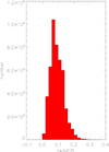 |
Fig. 1. Redshift distribution of low-redshift, narrow-emission-line galaxies. A total of 47 968 galaxies with reliable narrow emission lines are selected from SDSS DR16 using an SQL Search query. The redshifts range from 0.0002 to 0.3469. |
It is worth mentioning that, through the similar SQL Search queries, considering the Ke01 lines described by the flux ratios of different narrow emission lines in the BPT diagrams, 14 321 galaxies lying above the Ke01 line in the [N II] BPT diagram can be collected with reliable [N II] emission lines. Meanwhile, through the similar SQL Search queries, 12 250 galaxies lying above the Ke01 line in the [S II] BPT diagram can be collected with reliable [S II] emission lines, and 7309 galaxies lying above the Ke01 line in the [O II] BPT diagram can be collected with reliable [O I] emission lines. Therefore, in the BPT diagrams for the Seyferts and LINERs, the number of galaxies with reliable [N II] emission lines is 17% (96%) higher than those of galaxies with reliable [S II] ([O I]) emission lines, respectively. In other words, to determine a well-defined S-L line in the [N II] BPT diagram is more helpful for classifications of Seyferts and LINERs.
3. Main results
3.1. Current S-L lines in the [N II] BPT diagram
As the method shown and discussed in Kewley et al. (2006), the S-L lines can be determined and shown in the [S II] and [O I] BPT diagrams. Therefore, the same method was firstly applied to test its applicability in determining the S-L lines in the BPT diagrams based on our new sample of narrow emission line galaxies. Galaxy number count distributions with respect to the angle with log([S II]/Hα) and log([O I]/Hα) as the X-axis provided well double-peaked features similar to the Fig. 3 in Kewley et al. (2006), leading to the similar S-L lines in the [S II] and [O I] BPT diagrams as those reported in Kewley et al. (2006), as the detailed discussions in Appendix B. Unfortunately, the same method could not lead to an accepted S-L line in the [N II] BPT diagram, mainly because the galaxy number count distributions with respect to the angle with the log([N II]/Hα) as the X-axis were relatively even, failing to distinctly separate Seyferts from LINERs. More detailed discussions can be found in Appendix B.
Meanwhile, Schawinski et al. (2007) and Cid Fernandes et al. (2010) proposed S-L lines in the [N II] BPT diagram, which limited by their methods, can only be linear diagonal lines anyway. However, based on the Ke01 lines and the S-L lines reported in the [S II] and [O I] BPT diagrams (Kewley et al. 2001, 2006), 5791 Seyferts and 4228 LINERs, among our collected narrow emission line galaxies, that are consistently classified in both the [S II] and [O I] diagrams were collected. This approach ensures that only galaxies with unambiguous Seyfert or LINER classifications were used for further analysis in the [N II] diagram. These galaxies were then visualized in the [N II] BPT diagram, as shown by the semitransparent results in Fig. 2. Visually, they outlined a nonlinear S-L line between Seyferts and LINERs, with the potential to further classify Seyferts and LINERs in the composite galaxy region.
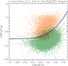 |
Fig. 2. Semitransparent visualization of the intersection boundary between Seyferts and LINERs in the [N II] BPT diagram. The nonlinear line in blue represents a simple outline of the intersection boundary determined by visual inspection. The plus signs in orange and hollow squares in dark green represent the Seyferts and LINERs that have been classified in both the [S II] and [O I] BPT diagrams, respectively. |
Therefore, at the current stage, the widely applied method in Kewley et al. (2006) cannot lead to an accepted S-L line in the [N II] BPT diagram, and the proposed Sc07 line and Fe10 line should be improved from linear diagonal lines to nonlinear lines. Here, in the paper, through the Seyferts and LINERs classified in the [S II] and/or [O I] BPT diagrams visualized in the [N II] BPT diagram, the expected intersection boundary between these two sub-classes of galaxies will be considered as the new and improved S-L line in the [N II] BPT diagram.
3.2. Our S-L results in the [N II] BPT diagram
Based on the classifications reported in the Kewley et al. (2006), the Seyferts and LINERs classified only in the [S II] BPT diagram, only in the [O I] diagram, in both the [S II] BPT diagram and the [O I] BPT diagram are visualized in the [N II] BPT diagram. Then, the one with the highest and most harmonious classification efficiency among the corresponding intersection boundaries of the Seyferts and the LINERs can be determined as the S-L line in the [N II] BPT diagram.
First of all, based on the 5966 Seyferts and 4919 LINERs classified in the [S II] BPT diagram well represented in the [N II] BPT diagram as the two contour maps shown in panel (a) of Fig. 3, the ridge line (if it exists) of their contour can be determined as the S-L line in the [N II] BPT diagram (the S line) by the following steps.
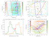 |
Fig. 3. Complete process for defining the S line. (a) shows the long-bin[19]. The contours with levels shown with colors from the color table of RED TEMPERATURE and from the color table of green-to-white LINEAR represent the results for the classified Seyferts and LINERs, respectively. The corresponding number densities of the contour levels are shown in the colorbars on both sides of the panel. The huge magenta asterisks represent the central points of the two contours. The magenta line represents the baseline. Two sets of parallel cyan lines divide the contour maps into 27 × 15 rectangle-bins. The boundaries of long-bin[19] are highlighted in blue. The boundaries of wider long-bins are highlighted in red. The red cross represents the intersection point of the Seyfert and LINER distributions within the long-bin[19]. (b) shows the rectangle-bin[19, 9]. The boundaries of rectangle-bin[19, 9] are highlighted in blue. The triangles in orange and the diamonds in dark green represent the Seyferts and LINERs classified in the [S II] BPT diagram, respectively. The red cross has the same meaning as that in panel (a). (c) shows the couple of histograms that depict the dependence of the percentage of Seyfert (orange) and LINER (dark green) counts within each rectangle-bin in long-bin[19] relative to their total counts in long-bin[19] on the displacement of each rectangle-bin in long-bin[19] from the bottom of long-bin[19]. The red arrow corresponds to the intersection point in long-bin[19], which matches the location of the thick red crosses in the previous two panels. (d) shows the final result of the S line (solid blue line) and its confidence bands (dashed blue lines). Magenta asterisks represent the collected intersection points from all the long-bins and wider long-bins. The solid red line is the Ke01 line. The dashed green line is the Ka03 line. |
For the first step, a magenta baseline is drawn to connect the central points of the contour maps for Seyferts and LINERs, marked by huge magenta asterisks at (−0.03, 0.14) and (−0.07, 0.61), respectively, as shown in panel (a) of Fig. 3. For the second step, 28 parallel lines are drawn along the direction of the baseline, with each line spaced 0.04 dex apart, dividing the contour maps for Seyferts and LINERs into 27 long-bins, as shown by an example long-bin[19] in panel (a) of Fig. 3. For the third step, 16 parallel lines are drawn in the direction perpendicular to the baseline, with each line spaced 0.09 dex apart, further subdividing each long-bin into 15 rectangle-bins, as shown by an example rectangle-bin[19, 10] in panel (b) of Fig. 3. The contour maps for Seyferts and LINERs are divided into 27 × 15 rectangle-bins, as shown in the grids in panel (a) of Fig. 3. Meanwhile, the number counts and average coordinates of the classified Seyferts and LINERs within each rectangle-bin can be easily obtained. In fact, grids denser or sparser than 28 × 16 were tested, yielding consistently similar results, except when the grids are extremely large or small, which results in either too few or too many Seyferts and LINERs located within the rectangle-bins. For the fourth step, a couple of histograms are drawn to depict the dependence of the percentages of Seyferts and LINERs counts within each rectangle-bin relative to their total counts in the corresponding long-bin on the displacement of each rectangle-bin from the bottom of the corresponding long-bin. A couple of example histograms are shown in panel (c) of Fig. 3. The average of the average coordinates of Seyferts and LINERs in the rectangle-bin corresponding to the local minimum point between the peaks of the two histograms is considered as the coordinates of the intersection point in each long-bin. In fact, due to the small sample sizes of Seyferts and LINERs, reasonable intersection points cannot be pinpointed from long-bin[1] to long-bin[2] and from long-bin[23] to long-bin[27]. In order to better pinpoint the intersection points near log([N II]/Hα) = 0.3 and −0.5, two wider long-bins are established, with boundaries marked in red in panel (a) of Fig. 3. Finally, the coordinates of the intersection points in all the long-bins and wider long-bins are pinpointed. Then, considering the nonlinear trend of the intersection points, a third-degree polynomial function, instead of a straight line, is applied using the poly_fit code without considering uncertainties to describe the intersection points, leading to the S line, which determines the intersection boundary between Seyferts and LINERs in the [N II] BPT diagram, as shown in panel (d) of Fig. 3, by the formula
![Mathematical equation: $$ \begin{aligned}\log &(\mathrm {{[O\ {{\small{\text{III}}}}]/H\beta }}) = 0.46 + 0.99 \times \log (\mathrm {{[N\ {{\small{\text{II}}}}]/H\alpha }}) \\ &+ 0.61 \times (\log (\mathrm {{[N\ {{\small{\text{II}}}}]/H\alpha }}))^2 - 1.11 \times (\log (\mathrm {{[N\ {{\small{\text{II}}}}]/H\alpha }}))^3. \end{aligned} $$](/articles/aa/full_html/2025/07/aa54434-25/aa54434-25-eq1.gif) (1)
(1)
Moreover, among the 21 613 galaxies above the Ka03 line in the [N II] BPT diagram, 6301 galaxies are classified as Seyferts and 15 312 as LINERs by the S line. In contrast, 7424 galaxies are classified as Seyferts and 14 189 as LINERs by the Sc07 line, while 6815 galaxies are classified as Seyferts and 14 798 as LINERs by the Fe10 line. Meanwhile, among the 9797 galaxies above the Ke01 line in the [N II] BPT diagram, 5866 galaxies are classified as Seyferts and 3931 as LINERs by the S line. In contrast, 6107 galaxies are classified as Seyferts and 3690 as LINERs by the Sc07 line, while 5838 galaxies are classified as Seyferts and 3959 as LINERs by the Fe10 line.
Similar to the S line determined above in the [N II] BPT diagram through the classified Seyferts and LINERs in the [S II] BPT diagram, another S-L line (the O line) in the [N II] BPT diagram can be determined through the classified Seyferts and LINERs in the [O I] BPT diagram as follows.
The 7550 Seyferts and 5620 LINERs classified in the [O I] BPT diagram are represented in the [N II] BPT diagram, and the aforementioned steps are repeated to determine the corresponding intersection boundary, referred to as the O line. The central points of the contour maps for Seyferts and LINERs are at coordinates (−0.10, 0.55) and (−0.07, 0.04). It is worth noting that when drawing parallel lines along the baseline direction, the spacing is adjusted to 0.02 dex, otherwise, the numbers of galaxies in the rectangle-bins will be too large. Moreover, three wider long-bins are established near log([N II]/Hα) = 0.2,−0.4 and −0.6, due to the existence of a significant number of Seyferts and LINERs. The detailed process is shown in Fig. 4, with the determined O line described by the formula
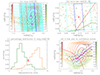 |
Fig. 4. Complete process for defining the O line. The symbols and line styles have the same meanings as those in Fig. 3, but Seyferts and LINERs are classified in the [O I] BPT diagram. |
![Mathematical equation: $$ \begin{aligned}\log &(\mathrm {{[O\ {{\small{\text{III}}}}]/H\beta }}) = 0.41 + 1.11 \times \log (\mathrm {{[N\ {{\small{\text{II}}}}]/H\alpha }}) \\ &+ 0.40 \times (\log (\mathrm {{[N\ {{\small{\text{II}}}}]/H\alpha }}))^2 - 1.22 \times (\log (\mathrm {{[N\ {{\small{\text{II}}}}]/H\alpha }}))^3.\end{aligned} $$](/articles/aa/full_html/2025/07/aa54434-25/aa54434-25-eq2.gif) (2)
(2)
Similarly, among the 21 613 galaxies located above the Ka03 line in the [N II] BPT diagram, 7624 galaxies are classified as Seyferts and 13 989 as LINERs by the O line. Meanwhile, among the 9797 galaxies located above the Ke01 line in the [N II] BPT diagram, 6405 galaxies are classified as Seyferts and 3392 as LINERs by the O line. As shown in panel (d) of Fig. 4, the O line has been presented in the [N II] BPT diagram.
Finally, similar to the S line and the O line determined above in the [N II] BPT diagram, another S-L line (the SO line) in the [N II] BPT diagram can be determined through the classified Seyferts and LINERs both in the [S II] BPT diagram and in the [O I] BPT diagram as follows.
The 5791 Seyferts and 4228 LINERs classified in both the [S II] and the [O I] BPT diagram are represented in the [N II] BPT diagram. The central points of the contour maps for Seyferts and LINERs are at coordinates (−0.03, 0.14) and (−0.07, 0.61). By repeating the aforementioned steps, with the detailed process shown in Fig. 5, a third S-L line is determined, referred to as the SO line, with the equation
 |
Fig. 5. Complete process for defining the SO line. The symbols and line styles have the same meanings as those in Fig. 3, but Seyferts and LINERs are classified in both the [S II] BPT diagram and the [O I] BPT diagram. |
![Mathematical equation: $$ \begin{aligned}\log &(\mathrm {{[O\ {{\small{\text{III}}}}]/H\beta }}) = 0.44 + 0.85 \times \log (\mathrm {{[N\ {{\small{\text{II}}}}]/H\alpha }}) \\ &+ 0.55 \times (\log (\mathrm {{[N\ {{\small{\text{II}}}}]/H\alpha }}))^2 - 0.82 \times (\log (\mathrm {{[N\ {{\small{\text{II}}}}]/H\alpha }}))^3.\end{aligned} $$](/articles/aa/full_html/2025/07/aa54434-25/aa54434-25-eq3.gif) (3)
(3)
Similarly, among the 21 613 galaxies located above the Ka03 line in the [N II] BPT diagram, 6493 galaxies are classified as Seyferts and 15 120 as LINERs by the SO line. Meanwhile, among the 9797 galaxies located above the Ke01 line in the [N II] BPT diagram, 6067 galaxies are classified as Seyferts and 3730 as LINERs by the SO line. As shown in panel (d) of Fig. 5, the SO line has been presented in the [N II] BPT diagram.
There are the following points that need to be declared.
-
First, taking the SO line as an example, the above procedures are repeated with samples at different scales to examine the impacts of selection effects, as well as the robustness of our method. 50% of the objects are randomly selected from Sample 1 as one new sample (Sample 2), and the other four samples (Samples 3–6) are constructed by adjusting the lower limits of the flux-to-uncertainty ratio or SNmedian for the fluxes in the SQL Search query. These operations lead to five new couples of Seyferts and LINERs samples. Detailed SQL condition adjustments and counts of Seyferts and LINERs are presented in Table 1. Subsequently, the same procedures used to determine the SO line (as shown in panel (a) of Fig. 6) are repeated, leading to five classification lines (as shown in panels (b), (c), (d), (e), and (f) of Fig. 6). It is evident that the intersection points in panels (b), (c), (d), (e), and (f) show no significant differences in position and trend compared to those in panel (a). This consistency indicates that, while different SQL search conditions introduce certain selection effects, their impacts on determining the SO line are negligible. Therefore, our method for classifying Seyferts and LINERs in the [N II] BPT diagram can be considered highly robust.
-
Second, multiple polynomial forms, from 2nd-degree to 5th-degree, have been systematically evaluated during the line fitting. Although the 4th-degree, and 5th-degree polynomial fits exhibit smaller RMS scatter, and χ2/d.o.f values, as shown in Table 2, they show unphysically sharp declines where log([NII]/Hα)>0.3, while the 2nd-degree polynomial fit shows an unphysically sharp increase in the same region, as shown in panel (a) of Fig. 6. In the region with a high density of intersection points, all fits perform comparably. However, although polynomial fits of 2nd, 4th, and 5th degrees may be valid within limited regimes, the 3rd-degree polynomial offers the best compromise between smoothness, physical plausibility, and performance across the entire parameter space, making it the most suitable choice.
-
Third, the orientations of the baselines have been adjusted several times by modifying the coordinates of the central points in the contour maps for Seyferts and LINERs, and the resulting intersection boundaries, obtained through repeated adjustments, show significant overlap, confirming the reliability of the results.
So far, we have five S-L lines in the [N II] BPT diagram, the S line, the O line, the SO line, the Sc07 line, and the Fe10 line. It is necessary to check which one is preferred.
 |
Fig. 6. Results of determining the SO line through the same procedure using different samples and the results of fitting the SO line using polynomial functions from 2nd to 5th degrees. Panel (a) presents the results of determining the SO line using sample 1 with polynomial functions from 2nd to 5th degrees. The symbols and line styles have the same meanings as those in Fig. 3. The large blue asterisks represent the central points of the two contours. The dashed black curve represents the 2nd-degree fit. The solid blue curve represents the 3rd-degree fit. The dashed purple curve represents the 4th-degree fit. The dashed red curve represents the 5th-degree fit. Panels (b), (c), (d), (e), and (f) present the results of determining the SO line using samples 2–6 with a 3rd-degree fit, respectively. The symbols and line styles have the same meanings as those in panel (a). |
Samples corresponding to various SQL conditions.
RMS scatters and χ2/d.o.f values for 2nd-5th degree polynomial fits.
4. Necessary discussions
In order to test the efficiency of the S line, the O line, the SO line, the Sc07 line, and the Fe10 line, three quantitative analyses are carried out as follows. Based on the results of the three tests, the best-performing S-L line, the SO line, is selected and validated using a SVM (support vector machine) technique. Finally, an application based on the SO line is presented.
4.1. Comparisons of number ratios FS and FL
For the first, the effectiveness of the S-L lines can be checked by the defined number ratios FS and FL, which are defined by
 (4)
(4)
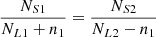
Here,  (
( ) is the total number of Seyferts (LINERs) classified in the [S II] and/or [O I] BPT diagrams and lying above the Ka03 (Ke01) line in the [N II] BPT diagram. In addition,
  (
( ) is the number of Seyferts (LINERs) classified in the [S II] and/or [O I] BPT diagrams and lying above the Ka03 (Ke01) line and also above (below) the given S-L line in the [N II] BPT diagram. A larger FS (FL) demonstrates that more Seyferts (LINERs) are classified into the same category through the given S-L line, indicating higher classification efficiency. Meanwhile, a smaller absolute difference of |FS−FL| for the S-L line indicates a more harmonious consistency in the classification efficiency of Seyferts and LINERs. The FS, FL and corresponding |FS−FL| for the S line, the O line, the SO line, the Sc07 line, and the Fe10 line are shown in Table 3, with detailed descriptions on the results as follows.
-
For the S line, Seyferts and LINERs are classified in the [S II] BPT diagram, with
 ,
,  ,
,  and
and  , based on the Ka03 line. Then,
  and
and  , with an absolute difference of |FS−FL| = 0.24%.
 -
For the O line, Seyferts and LINERs are classified in the [O I] BPT diagram, with
 ,
,  ,
,  and
and  , based on the Ka03 line. Then,
  and
and  , with an absolute difference of |FS−FL| = 2.57%.
 -
For the SO line, Seyferts and LINERs are classified in the [S II] and [O I] BPT diagram, with
 ,
,  ,
,  and
and  , based on the Ka03 line. Then,
  and
and  , with an absolute difference of |FS−FL| = 0.67%. The FS and FL for the SO line are the largest among the results for the S line, the O line, and the SO line, with a small enough absolute difference of |FS−FL|.
 -
For the Sc07 line, Seyferts and LINERs are classified in both the [S II] diagram and the [O I] BPT diagram, with
 ,
,  ,
,  and
and  , based on the Ka03 line. Then,
  and
and  , with an absolute difference of |FS−FL| = 4.46%. Although FS = 94.58% is 0.65% larger than that for the SO line, the absolute difference for the Sc07 line is 3.79% larger than that for the SO line.
 -
For the Fe10 line, Seyferts and LINERs are classified in the [S II] and [O I] BPT diagram, with
 ,
,  ,
,  and
and  , based on the Ka03 line. Then,
  and
and  , with an absolute difference of |FS−FL| = 0.21%. Although the absolute difference for the Fe10 line is the smallest among all the S-L lines, the FS and FL for the Fe10 line are 1.33% and 1.79% smaller than those for the SO line, respectively.
 -
For the S line, Seyferts and LINERs are classified in the [S II] BPT diagram, with
 ,
,  ,
,  and
and  , based on the Ke01 line. Then,
  and
and  , with an absolute difference of |FS−FL| = 3.17%.
 -
For the O line, Seyferts and LINERs are classified in the [O I] BPT diagram, with
 = 6544,
  ,
,  and
and  , based on the Ke01 line. Then,
  and
and  , with an absolute difference of |FS−FL| = 2.61%.
 -
For the SO line, Seyferts and LINERs are classified in the [S II] and [O I] BPT diagram, with
 = 5574,
  = 2814,
  = 5273 and
  = 2623, based on the Ke01 line. Then,
  = 94.60% and
  = 93.21%, with an absolute difference of |FS−FL| = 1.39%. The FS and FL for the SO line are the largest among the results for the S line, the O line, and the SO line, with the smallest absolute difference of |FS−FL|.
 -
For the Sc07 line, Seyferts and LINERs are classified in both the [S II] diagram and the [O I] BPT diagram, with
 = 5574,
  = 2814,
  = 5272 and
  = 2622, based on the Ka03 line. Then,
  = 94.58% and
  = 93.18%, with an absolute difference of |FS−FL| = 1.41%. Although FS and FL are the closest to those for the SO line, the absolute difference for the Sc07 line is 0.02% larger than that for the SO line.
 -
For the Fe10 line, Seyferts and LINERs are classified in the [S II] and [O I] BPT diagram, with
 = 5574,
  = 2814,
  = 5167 and
  = 2677, based on the Ke01 line. Then, FS =
 = 92.70% and FL =
 = 95.13%, with an absolute difference of |FS−FL| = 2.43%. Although FL = 95.13% is 1.92% larger than that for the SO line, the absolute difference for the Fe10 line is 1.04% larger than that for the SO line.
Number ratios FS and FL of S-L lines.
Both FS and FL contributed by the SO line are the largest and consistent enough, whether analyzed based on the Ka03 line or the Ke01 line, compared to those contributed by the S line and the O line. Considering the SO line, Sc07 line, and Fe10 line, although neither the FS based on the Ka03 line nor the FS based on the Ke01 line contributed by the SO line is the largest, the SO line shows the best balance between efficiency and consistency overall for achieving high and consistent FS and FL with a relatively small |FS−FL|, making it the most reliable among the three.
4.2. Comparisons of FS/FL
For the second, the ratios of FS/FL along each S-L line have been calculated to examine the relative stability of the S-L lines. In the previous section, the absolute classification efficiencies of the S-L lines for Seyferts and LINERs are compared in regions above the Ka03 (Ke01) line to assess the global classification efficiency of different S-L lines. However, the comparisons of absolute efficiency cannot reveal the classification efficiency of the S-L lines in local regions and their stability along the S-L lines. To further investigate the classification efficiency of the S-L lines in various local regions and their stability, the S-L lines are divided into several local regions based on different ways, and the FS and FL values for these regions are calculated separately. By analyzing the variation of the ratios of FS/FL in these local regions, the stability of the classification efficiency of each S-L line across the overall range is further compared. Through the previous comparison of the absolute efficiency using FS and FL, the SO line clearly outperforms the S line and O line. The S line and O line, while useful for classification, are excluded from this comparison due to their lower classification efficiency than the SO line.
The 5791 Seyferts and 4228 LINERs classified in both the [S II] and the [O I] BPT diagram are represented in the [N II] BPT diagram. As shown in panel (a) of Fig. 7, the long-bins defined in Section 3.2 divided the contour maps for Seyferts and LINERs into 27 groups along the S-L lines. Meanwhile, as shown in panels (b) and (c) of Fig. 7, 25 arcs in cyan are translated 0.04 dex equally by Ke01 line and Ka03 line along the direction of log([O III]/Hβ) = log([N II]/Hα), dividing the contour maps for Seyferts and LINERs into 24 Ke-long-bins and Ka-long-bins along the S-L lines, respectively. Then the values of FS/FL within each long-bin, Ke-long-bin, and Ka-long-bin are calculated. The dependencies of FS/FL on the long-bins, Ke-long-bins, and Ka-long-bins are shown in panels (d), (e), and (f) of Fig. 7, respectively.
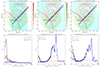 |
Fig. 7. Process and results for testing the dependencies of FS/FL on long-bins, Ke-long-bins, and Ka-long-bins. (a) shows long-bins in the [N II] BPT diagram. The contours with levels shown with colors from the color table of RED TEMPERATURE and from the color table of green-to-white LINEAR represent the results for the Seyferts and LINERs classified in the [S II] and [O I] BPT diagram, respectively. The corresponding number densities of the contour levels are shown in the colorbars on both sides of panel (b). The 28 lines in cyan represent the boundaries of long-bins. The solid red line is the Ke01 line. The dashed green line is the Ka03 line. The solid purple line is the Sc07 line. The solid black line is the Fe10 line. The solid blue line is the SO line. (b) shows Ke-long-bins in the [N II] BPT diagram. The symbols and line styles have the same meanings as those in panel (a), but the 25 arcs in cyan represent the boundaries of Ke-long-bins. (c) shows Ka-long-bins in the [N II] BPT diagram. The symbols and line styles have the same meanings as those in panel (a), but the 25 arcs in cyan represent the boundaries of Ka-long-bins. (d) shows the dependence of FS/FL for S-L lines on long-bins. The colors of the polylines correspond to the colors of the S-L lines in panel (a), purple for the Sc07 line, black for the Fe10 line, and blue for the SO line. The red horizontal line indicates log([N II]/Hα) = 1. (e) shows the dependence of FS/FL for S-L lines on Ke-long-bins. The other symbols and line styles have the same meanings as those in panel (d). (f) shows the dependence of FS/FL for S-L lines on Ka-long-bins. The other symbols and line styles have the same meanings as those in panel (d). |
It is obvious that the FS/FL for the SO line, the Sc07 line, and the Fe10 line show no obvious difference in the region far above the Ke01 line (log([N II]/Hα) larger than 0). However, regardless of long-bins, Ke-long-bins, or Ka-long-bins, the FS/FL for the SO line in the composite galaxy region, which is above the Ka03 line and below the Ke01 line, is much closer to 1 than for those for the Sc07 line and the Fe10 line, indicating the consistency of the efficiency of the SO line in classifying Seyferts and LINERs in the composite galaxy region and the region above the Ke01 line.
4.3. Comparisons of confidence bands
For the third, besides the effectiveness of the S-L lines checked by FS and FL and their stability checked by FS/FL, confidence bands have been determined for S-L lines. The upper boundary of the confidence bands ensures that LINERs classified in the [S II] and [O I] BPT diagram above the Ka03 line and above this line account for not larger than 2% of the total LINERs classified in the [S II] and [O I] BPT diagram above the Ka03 line. Meanwhile, the lower boundary of the confidence bands ensures that Seyferts classified in the [S II] and [O I] BPT diagram above the Ka03 line and below this line account for not larger than 2% of the total Seyferts classified in the [S II] and [O I] BPT diagram above the Ka03 line, as shown in panels (d) of Fig. 3, Fig. 4, Fig. 5. The initial threshold is set at 99.73% (3σ), however, several points in the remaining 0.27% that are far from the main distribution of the [N II] BPT diagram could significantly interfere with the positions of the confidence bands, making the comparisons less meaningful. Meanwhile, the S-L lines can accurately classify approximately 96% of Seyferts and LINERs as the largest FS and FL are around 94%, therefore, the threshold should be set above 96%. Consequently, the threshold is adjusted to 98% (2.33σ) to ensure the confidence bands are reliable and comparable.
The upper and lower boundaries of the confidence bands for the S line are obtained by the S line plus 0.1486 and minus 0.1105, respectively. For the O line, the upper and lower boundaries of the confidence bands are obtained by the O line plus 0.1930 and minus 0.1880, respectively. The upper and lower boundaries of the confidence bands for the Sc07 line are obtained by the Sc07 line plus 0.1748 and minus 0.0824, respectively. For the Fe10 line, the upper and lower boundaries of the confidence bands are obtained by the Fe10 line plus 0.1300 and minus 0.1110, respectively. Impressively, for the SO line, the upper and lower boundaries of the confidence bands are obtained by the SO line plus 0.0935 and minus 0.0800 merely, respectively. The upward, downward and total (upward + downward) shift distances of the S-L lines are presented in Table 4.
Upward, downward, and total shift distances of S-L lines for obtaining confidence bands.
The smallest total shift distance of the upper and lower boundaries of the confidence bands for the SO line makes the SO line far superior to the other S-L lines, as shown in Fig. 8.
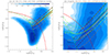 |
Fig. 8. Comparison of all the versions of the S-L lines and their confidence bands mentioned in this paper, in the [N II] BPT diagram. (a) shows the S line (solid green line), the O line (solid orange line), the SO line (solid yellow line), the Sc07 line (solid purple line), and the Fe10 line (solid black line), and the corresponding confidence bands in dashed lines in the same color. The Ke01 line and the Ka03 line have the same line styles as in Fig. 3. The contour filled with bluish colors represents the results for the sample of our collected galaxies. The corresponding number densities of the different colors are shown in the colorbar on the top of the panel. (b) shows the S-L lines in the [N II] BPT diagram within smaller limited ranges of log([N II]/Hα) and log([O III]/Hβ). |
4.4. Optimal choice
Considering the above aspects, the SO line is preferred in the [N II] BPT diagram. Moreover, as described in Section 2, we have demonstrated through SQL search queries that the number of galaxies with reliable [N II] emission lines is much higher than those of galaxies with reliable [S II] or [O I] emission lines. This indicates that the calibrated SO line in the [N II] BPT diagram can help classify a large number of galaxies more precisely and efficiently into Seyferts and LINERs in the [N II] BPT diagram.
It is worth noting that Maragkoudakis et al. (2014) have pointed out that the positions of a galaxy in the BPT diagrams can vary with the aperture used for observation, since at low redshifts (z<0.45), only the inner zones of galaxies can be captured, rather than their full extents. To examine the impacts of aperture effects on our results, which is collected from SDSS DR16 spectra using a fixed 1.5″-radius fiber aperture, the physical area captured by a 1.5″-radius aperture is compared with the typical size of the narrow line region (NLR).
First, the physical radius corresponding to a 1.5″-radius aperture ( ) can be calculated with the redshift (z). Second, Liu et al. (2013) have provided a correlation between the size of the NLR and [O III] line luminosity (L[O III], expressed in 1042 erg s−1):
![Mathematical equation: $$ \log (R_{{\mathrm {[O\ {{\small{\text{III}}}}]}}}) = 0.250 \log (L_{{\mathrm {[O\ {{\small{\text{III}}}}]}}}) + 3.746, $$](/articles/aa/full_html/2025/07/aa54434-25/aa54434-25-eq78.gif) (5)
(5)
where R[O III] is the radius of the NLR of [O III] emission line, expressed in parsecs.
The distribution of the ratio ![Mathematical equation: $ R_{1.5^{{\prime\prime}}} / R_{{\mathrm {[O\ {{\small{\text{III}}}}]}}} $](/articles/aa/full_html/2025/07/aa54434-25/aa54434-25-eq79.gif) for each object is subsequently calculated and shown in Fig. 9. Among our sample 1, the ratios of
for each object is subsequently calculated and shown in Fig. 9. Among our sample 1, the ratios of  to R[O III] for 37 188 (78%) objects are greater than 1, for which the NLRs are fully captured by the 1.5″ aperture. Nevertheless, there should be caution when applying the SO line to datasets with significantly different apertures.
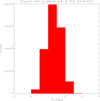 |
Fig. 9. Distribution of the ratio |
![Mathematical equation: $ R_{1.5^{{\prime\prime}}} / R_{\mathrm {[O\ {{\small{\text{III}}}}]}} $](/articles/aa/full_html/2025/07/aa54434-25/aa54434-25-eq81.gif)
4.5. Application of the SVM technique
The SVM is a class of supervised learning methods widely used for classifications, especially binary classifications. The SVM supports various kernel functions that can nonlinearly map input vectors into a high-dimensional feature space, where nonlinear problems become linearly separable (Schölkopf et al. 1998; Hearst et al. 1998). In the feature space, the SVM determines the coefficients of the linear hyperplane through the optimization of the Lagrangian multiplier, thereby constructing an optimal hyperplane (decision boundary) that maximizes the margin between support vectors (Cortes & Vapnik 1995). More detailed introductions to SVM are available on the scikit-learn SVM module page2.
Applying the SVM to classify Seyferts and LINERs in the [N II] BPT diagram offers an independent test of the validity of the SO line. Specifically, based on Sample 1, objects classified as Seyferts or LINERs consistently in both the [S II] and [O I] BPT diagrams are selected, and their [O III]/Hβ and [N II]/Hα ratios are collected and labeled as 1 (Seyferts) and 0 (LINERs), respectively. These two sets of data are then standardized and input into the SVM model. The kernel is set to poly with degree = 3, and the penalty parameter is fixed at the default value C = 1. The resulting decision boundary is the SVM classification line between Seyferts and LINERs in the [N II] BPT diagram, as shown by the solid blue curve in Fig. 10. Objects located within the margin (between the dashed blue curves) are considered to have low classification confidence. The same procedures are then applied to Samples 3 and 4, resulting in two additional SVM classification lines. Above the Ka03 line, the positions and shapes of the three SVM classification lines are all in good agreement with the SO line, providing strong support for the SO line and further confirming that the selection effects have little impact on determining the SO line.
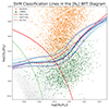 |
Fig. 10. Three SVM classification lines for Seyferts and LINERs in the [N II] BPT diagram. The solid orange and dark green circles represent the Seyferts and LINERs consistently classified in both the [S II] BPT diagram and the [O I] BPT diagram using Sample 1. The solid red line is the Ke01 line. The dashed green line is the Ka03 line. The dashed red line is the SO line. The solid blue, cyan, and magenta lines represent the SVM classification lines obtained using Samples 1, 3, and 4, respectively. The dashed lines of the corresponding color represent the upper and lower boundaries of margins. |
4.6. Basic applications of SO line
The proposed and preferred SO line in the [N II] BPT diagram is then applied to the following project. Similar to the criteria in Section 2 (redshift z<0.35, narrow emission line fluxes of [O III]λ5007 Å, Hβ, [N II]λ6586 Å, and Hα being 5 times larger than their corresponding uncertainties which are greater than 0, and the median S/N per pixel for the restframe 6400–6765 Å and 4750–4950 Å regions, which are near the Hα and Hβ emission lines, being greater than 10), there are 2703 quasars (Type-1 AGNs) being collected from the quasar catalog reported by Shen et al. (2011), which is distributed as a FITS file. Our analysis specifically utilizes the following fields in the FITS file:
REDSHIFT,
LOGL_OIII_5007, LOGL_OIII_5007_ERR,
LOGL_NARROW_HB, LOGL_NARROW_HB_ERR,
LOGL_NII_6585, LOGL_NII_6585_ERR,
LOGL_NARROW_HA, LOGL_NARROW_HA_ERR,
LINE_MED_SN_HA, LINE_MED_SN_HB.
Then, the Type-1 AGNs collected from Shen et al. (2011) and all the Type-2 objects in sample 1 are shown in the [N II] BPT diagram, respectively. Those objects located above the Ka03 (Ke01) line and above the SO line in the [N II] BPT diagram are classified as Type-1 and Type-2 Seyferts, respectively, while those located above the Ka03 (Ke01) line but below the SO line are classified as Type-1 and Type-2 LINERs. The number counts of Type-1 Seyferts (NS1 = 2311 (2239)), Type-2 Seyferts (NS2 = 6261 (6067)), Type-1 LINERs (NL1 = 193 (108)) and Type-2 LINERs (NL2 = 5206 (3730)) have been calculated. The numbers out of parentheses correspond to the number counts obtained based on the application of the SO line combined with the Ka03 line, while those in the parentheses correspond to the number counts obtained based on the application of the SO line combined with the Ke01 line. These results are highlighted in green and red respectively in panels (a) and (b) of Fig. 11, and are also listed in the third and seventh rows of Table 5. It is worth mentioning that in the composite galaxy region (above the Ke01 line and below the Ka03 line in the [N II] BPT diagram), only objects that are lying above the Ke01 lines in the [S II] and [O I] BPT diagrams are selected. Without these constraints, the numbers of Type-2 LINERs increase by approximately 10 000 objects, while those of Type-2 Seyferts increase by only around 1000, as shown in Section 3.2. This selection ensures more reliable Type-2 LINER samples in the composite galaxy region by reducing objects that fail to meet AGN criteria using three BPT diagrams.
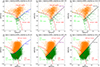 |
Fig. 11. Distributions and number counts of Type-1 Seyferts and Type-1 LINERs, as well as Type-2 Seyferts and Type-2 LINERs, classified by the SO line, Sc07 line, and the Fe10 line, respectively, combined with the Ke01 (Ka03) line, in the [N II] BPT diagram. (a) shows the distributions of Type-1 Seyferts and Type-1 LINERs classified by the SO line, combined with the Ke01 (Ka03) line, in the [N II] BPT diagram. The samples of Type-1 Seyferts (plus signs in orange) and Type-1 LINERs (hollow squares in dark green) are collected from the quasars catalog proposed by Shen et al. (2011). The solid red line is the Ke01 line. The dashed green line is the Ka03 line. The solid blue line is the SO line. The text highlighted in red (green) represents the number counts of Type-1 Seyferts and Type-1 LINERs classified by the SO line combined with the Ke01 (Ka03) line. (b) shows the distributions of Type-2 Seyferts and Type-2 LINERs classified by the SO line, combined with the Ke01 (Ka03) line, in the [N II] BPT diagram, while also considering the classification results of the Ke01 lines in the [S II] and [O I] BPT diagrams. The samples of Type-2 Seyferts (plus signs in orange) and Type-2 LINERs (hollow squares in dark green) are collected in Section 2. The other symbols and line styles have the same meanings as those in panel (a). (c) shows the distributions of Type-1 Seyferts and Type-1 LINERs classified by the Sc07 line, combined with the Ke01 (Ka03) line, in the [N II] BPT diagram. The solid purple line is the Sc07 line. The other symbols and line styles have the same meanings as those in panel (a). (d) shows the distributions of Type-2 Seyferts and Type-2 LINERs classified by the Sc07 line, combined with the Ke01 (Ka03) line, in the [N II] BPT diagram, while also considering the classification results of the Ke01 lines in the [S II] and [O I] BPT diagrams. The solid purple line is the Sc07 line. The other symbols and line styles have the same meanings as those in panel (b). (e) shows the distributions of Type-1 Seyferts and Type-1 LINERs classified by the Fe10 line, combined with the Ke01 (Ka03) line, in the [N II] BPT diagram. The solid black line is the Fe10 line. The other symbols and line styles have the same meanings as those in panel (a). (f) shows the distributions of Type-2 Seyferts and Type-2 LINERs classified by the Fe10 line, combined with the Ke01 (Ka03) line, in the [N II] BPT diagram, while also considering the classification results of the Ke01 lines in the [S II] and [O I] BPT diagrams. The solid black line is the Fe10 line. The other symbols and line styles have the same meanings as those in panel (b). |
Number counts and ratios of Seyferts and LINERs classified by S-L Lines in our basic applications.
As our preliminary results, based on the application of the SO line combined with the Ka03 (Ke01) line, the number ratio of Type-1 Seyferts to Type-1 LINERs (NS1/NL1 = 11.97 (20.73)) is 9.98 (12.72) times greater than that of Type-2 Seyferts to Type-2 LINERs (NS2/NL2 = 1.20 (1.63)). As shown in the third and seventh rows of Table 5, these results provide further clues to support that about 89.96% (92.15%) of objects should be excluded from the Type-2 LINER sample or reclassified. Meanwhile, the number ratios of Type-1 Seyferts to Type-1 LINERs and Type-2 Seyferts to Type-2 LINERs based on the Sc07 line and Fe10 line have also been calculated. Based on the application of the Sc07 line combined with the Ka03 (Ke01) line, the calculated NS1/NL1 = 12.04 (15.53) is 8.99 (9.36) times larger than NS2/NL2 = 1.34 (1.66), while based on the application of the Fe10 line combined with the Ka03 (Ke01) line, the calculated NS1/NL1 = 11.58 (16.26) is 9.73 (11.06) times larger than NS2/NL2 = 1.19 (1.47). As shown in panels (c), (d), (e), and (f) of Fig. 11 and the fourth, fifth, eighth, and ninth rows of Table 5, these results indicate that the same proportion of objects should be excluded from the Type-2 LINER sample or reclassified compared to the SO line.
For the differences in the two number ratios, at least three points can be made to explain this.
-
First, as mentioned in Section 1, a significant fraction of objects in the Type-2 LINER sample are indeed non-AGN-related. Although these non-AGN-related LINERs lie above the Ke01 (Ka03) line and below the SO line in the [N II] BPT diagram, they should not be included in AGN statistics. Therefore, when calculating the number ratio of Type-2 Seyferts to Type-2 LINERs, they should be excluded. Under the assumption that part of Type-2 LINERs are non-AGN-related, considering that some objects should be excluded from the Type-2 LINER sample could be naturally applied to explain the number ratio of Type-2 Seyferts to Type-2 LINERs, which is quite different from that of Type-1 Seyferts to Type-1 LINERs, as follows.
In calculating the proportions of objects that should be excluded from the Type-2 LINER samples or reclassified (
 ), the following formula is used:
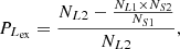 (6)
(6)and the resulting values are presented in column 8 of Table 5. By this formula, the percentage of the difference between the actual count (NL2) and the theoretical count (
 , based on the assumption that NS1/NL1 = NS2/NL2, and the resulting values are presented in column 9 of Table 5) of Type-2 LINERs relative to the actual count is quantified.
Based on the application of the defined SO line combined with the Ka03 (Ke01) line, if there are 89.96% (92.15%) Type-2 LINERs that are non-AGN-related, the number ratio of Type-2 Seyferts to Type-2 LINERs should be about 6261:523 = 11.97 (6067:293 = 20.71), leading to the same number ratio of Type-1 Seyferts to Type-1 LINERs being 2311:193 = 11.97 (2239:108 = 20.73). Similarly, based on the application of the proposed Sc07 line combined with the Ka03 (Ke01) line, if there are 88.88% (89.34%) Type-2 LINERs that are non-AGN-related, the number ratio of Type-2 Seyferts to Type-2 LINERs should be about 6565:545 = 12.05 (6107:393 = 15.54), leading to the same number ratio of Type-1 Seyferts to Type-1 LINERs being 2312:192 = 12.04 (2205:142 = 15.53). Based on the application of the proposed Fe10 line combined with the Ka03 (Ke01) line, if there are 89.77% (90.93%) Type-2 LINERs that are non-AGN-related, the number ratio of Type-2 Seyferts to Type-2 LINERs should be about 6219:537 = 11.58 (5838:359 = 16.26), leading to the same number ratio of Type-1 Seyferts to Type-1 LINERs being 2305:199 = 11.58 (2211:136 = 16.26). The data in this paragraph are shown in Table 5.
Daoutis et al. (2025) have demonstrated that 72% of LINERs are ionized predominantly by old stellar populations rather than AGN activity, through random forest machine learning combined with the D4000 continuum break index and Hα, [O III]λ5007 Å, and [N II]λ6584 Å emission-line features, which is broadly consistent with the above results.
-
Second, part of objects classified as Type-2 LINERs in the [N II] BPT diagram may actually be true Type-2 AGNs, as several candidates reported by Li et al. (2015), Shi et al. (2010), and Zhang et al. (2021), and two samples of candidates reported by Zhang (2014) and Pons & Watson (2016). In the framework of the unified model of AGNs, the true Type-2 AGNs have the same orientation as Type-1 AGNs, with unobscured central regions despite the absence of broad emission lines. Under the assumption that all the objects in the existing Type-2 LINER sample are AGN-related, since the non-AGN-related LINERs mentioned earlier cannot currently be precisely dismissed, considering part of the objects in the Type-2 LINER sample as Type-1 LINER candidates could be naturally applied to explain the number ratio of Type-2 Seyferts to Type-2 LINERs, which is quite different from that of Type-1 Seyferts to Type-1 LINERs, as follows.
If the numbers of objects expected to be reclassified from the Type-2 LINER samples to the Type-1 LINER samples are n1, then the equation
 (7)
(7)should hold, with the resulting values presented in column 10 of Table 5.
Based on the application of the defined SO line combined with the Ka03 (Ke01) line, if there are 1263 (927) Type-2 LINERs that can be reclassified as Type-1 LINERs, the number ratio of Type-2 Seyferts to Type-2 LINERs should be about 6261:3943 = 1.59 (6067:2803 = 2.16), leading to the same number ratio of Type-1 Seyferts to Type-1 LINERs being 2311:1456 = 1.59 (2239:1035 = 2.16). Similarly, based on the application of the proposed Sc07 line combined with the Ka03 (Ke01) line, if there are 1135 (875) Type-2 LINERs that can be reclassified as Type-2 Seyferts, the number ratio of Type-2 Seyferts to Type-2 LINERs should be about 6565:3767 = 1.74 (6107:2815 = 2.17), leading to the same number ratio of Type-1 Seyferts to Type-1 LINERs being 2312:1327 = 1.74 (2205:1017 = 2.17). Based on the application of the proposed Fe10 line combined with the Ka03 (Ke01) line, if there are 1274 (989) Type-2 LINERs that can be reclassified as Type-2 Seyferts, the number ratio of Type-2 Seyferts to Type-2 LINERs should be about 6219:3974 = 1.56 (5838:2970 = 1.97), leading to the same number ratio of Type-1 Seyferts to Type-1 LINERs being 2305:1473 = 1.56 (2211:1125 = 1.97).
-
Third, according to Mo et al. (2024), based on the Mapping Nearby Galaxies at Apache Point Observatory survey, a fading AGN exhibits LINER-like ionization in its central region while showing Seyfert-like emission in the outskirts. This suggests that some AGNs might lie above the Ke01 line and below the SO line in the [N II] BPT diagram and be classified as LINERs, with their Seyfert-like nature potentially masked by the central LINER-like properties. Consequently, part of objects in the Type-2 LINER sample might need to be reclassified into the Type-2 Seyfert sample. Similarly, under the assumption that all the objects in the existing Type-2 LINER sample are AGN-related, considering that part of the objects in the Type-2 LINER sample as Type-2 Seyfert candidates could be naturally applied to explain the number ratio of Type-2 Seyferts to Type-2 LINERs, which is quite different from that of Type-1 Seyferts to Type-1 LINERs, as follows.
If the numbers of objects expected to be reclassified from the Type-2 LINER samples to the Type-2 Seyfert samples are n2, then the equation
 (8)
(8)should hold, with the resulting values presented in column 11 of Table 5.
Based on the application of the defined SO line combined with the Ka03 (Ke01) line, if there are 4322 (3279) Type-2 LINERs that can be reclassified as Type-2 Seyferts, the number ratio of Type-2 Seyferts to Type-2 LINERs should be about 10 583:884 = 11.97 (9346:451 = 20.72), leading to the same number ratio of Type-1 Seyferts to Type-1 LINERs being 2311:193 = 11.97 (2239:108 = 20.73). Similarly, based on the application of the proposed Sc07 line combined with the Ka03 (Ke01) line, if there are 4023 (3097) Type-2 LINERs that can be reclassified as Type-2 Seyferts, the number ratio of Type-2 Seyferts to Type-2 LINERs should be about 10 588:879 = 12.05 (9204:593 = 15.52), leading to the same number ratio of Type-1 Seyferts to Type-1 LINERs being 2312:192 = 12.04 (2205:142 = 15.53). Based on the application of the proposed Fe10 line combined with the Ka03 (Ke01) line, if there are 4337 (3391) Type-2 LINERs that can be reclassified as Type-2 Seyferts, the number ratio of Type-2 Seyferts to Type-2 LINERs should be about 10 556:911 = 11.59 (9229:568 = 16.25), leading to the same number ratio of Type-1 Seyferts to Type-1 LINERs being 2 305:199 = 11.58 (2211:136 = 16.26).
At this stage, for the applications of the three methods to approximately 90% of the objects in the Type-2 LINER sample, aimed at achieving consistency between the number ratio of Type-2 Seyferts to Type-2 LINERs and that of Type-1 Seyferts to Type-1 LINERs, it remains unclear which of the methods, or a combination of them, is responsible, and the respective contribution of each. Detailed discussions on comparisons between Type-2 LINERs and Type-1 LINERs in larger samples can be found in our being prepared paper in the near future.
5. Main summary and conclusions
We obtained satisfactory results for the S-L lines in the [S II] and [O I] BPT diagrams using our high-quality samples, which are consistent with Kewley et al. (2006). However, we could not obtain distinct double-peaked features, making it unfeasible to define the S-L line in the [N II] BPT diagram. Meanwhile, the Sc07 proposed by Schawinski et al. (2007) and the Fe10 proposed by Cid Fernandes et al. (2010) in the [N II] BPT diagram are all linear and different, while a nonlinear line is visually better to describe the intersection boundary for Seyferts and LINERs. To address this, we propose a new method, which results in our improved Seyfert-LINER classification line, the SO line. With the more precise SO line, galaxies with weak [S II] or [O I] narrow forbidden emission lines but apparent [N II] emission lines can be well classified in the [N II] BPT diagram. This significantly enhances the efficiency of classifications between Type-2 Seyferts and Type-2 LINERs, compared to the Sc07 line and the Fe10 line, and leads to cleaner and larger samples of Type-2 Seyferts and Type-2 LINERs. Additionally, the representativeness of Sample 1 and the robustness of the new method are confirmed by excluding the impact of selection and aperture effects. We achieved this by adjusting the lower limits of the flux-to-uncertainty ratio or SNmedian, and by testing the  /R[O III] ratio, respectively. We further validated the reliability of the SO line using the SVM technique.
In our basic application, through the proposed SO line, we created cleaner samples of Type-1 Seyferts and LINERs and Type-2 Seyferts and LINERs, and the number ratio of Type-2 Seyferts to Type-2 LINERs is obviously different from that of Type-1 Seyferts to Type-1 LINERs. This indicates that about 90% Type-2 LINERs are non-AGN-related, true Type-2 AGNs, or objects that exhibit both Seyfert and LINER characteristics. In the near future, cleaner samples of Type-1 and Type-2 LINERs can be used to provide further clues on the probable number ratio of AGN-related LINERs to non-AGN-related LINERs, and cleaner samples of Type-1 and Type-2 Seyferts can be used to test the unified model of AGNs with as little effect from LINERs as possible.
Acknowledgments
We gratefully acknowledge the anonymous referee for giving us constructive comments and suggestions to greatly improve the paper. Zhang gratefully acknowledges the kind financial support from GuangXi University, and the grant support from NSFC-12173020 and NSFC-12373014. Cheng & Chen gratefully acknowledge the kind grant support from Innovation Project of Guangxi Graduate Education YCSW2024006. This paper has made use of the data from the SDSS projects (http://www.sdss3.org/), managed by the Astrophysical Research Consortium for the Participating Institutions of the SDSS-III Collaborations and the poly_fit code.
References
- Agostino, C. J., & Salim, S. 2019, ApJ, 876, 12 [NASA ADS] [CrossRef] [Google Scholar]
- Agostino, C. J., Salim, S., Faber, S. M., et al. 2021, ApJ, 922, 156 [NASA ADS] [CrossRef] [Google Scholar]
- Agostino, C. J., Salim, S., Boquien, M., et al. 2023a, MNRAS, 526, 4455 [NASA ADS] [CrossRef] [Google Scholar]
- Agostino, C. J., Salim, S., Ellison, S. L., Bickley, R. W., & Faber, S. M. 2023b, ApJ, 943, 174 [NASA ADS] [CrossRef] [Google Scholar]
- Ahumada, R., Allende Prieto, C., Almeida, A., et al. 2020, ApJS, 249, 3 [NASA ADS] [CrossRef] [Google Scholar]
- Antonucci, R. 1993, ARA&A, 31, 473 [Google Scholar]
- Baldwin, J. A., Phillips, M. M., & Terlevich, R. 1981, PASP, 93, 5 [Google Scholar]
- Bremer, M., Scharwächter, J., Eckart, A., et al. 2013, A&A, 558, A34 [NASA ADS] [CrossRef] [EDP Sciences] [Google Scholar]
- Brinchmann, J., Charlot, S., White, S. D. M., et al. 2004, MNRAS, 351, 1151 [Google Scholar]
- Bruzual, G., & Charlot, S. 2003, MNRAS, 344, 1000 [NASA ADS] [CrossRef] [Google Scholar]
- Cid Fernandes, R., Schlickmann, M., Stasinska, G., et al. 2009, in The Starburst-AGN Connection, eds. W. Wang, Z. Yang, Z. Luo, & Z. Chen, ASP Conf. Ser., 408, 122 [Google Scholar]
- Cid Fernandes, R., Stasińska, G., Schlickmann, M. S., et al. 2010, MNRAS, 403, 1036 [Google Scholar]
- Coldwell, G. V., Alonso, S., Duplancic, F., & Mesa, V. 2018, MNRAS, 476, 2457 [Google Scholar]
- Contini, M., & Viegas, S. M. 2001, ApJS, 132, 211 [NASA ADS] [CrossRef] [Google Scholar]
- Cortes, C., & Vapnik, V. 1995, Mach. Learn., 20, 273 [Google Scholar]
- Daoutis, C., Zezas, A., Kyritsis, E., Kouroumpatzakis, K., & Bonfini, P. 2025, A&A, 693, A95 [NASA ADS] [CrossRef] [EDP Sciences] [Google Scholar]
- de Souza, R. S., Dantas, M. L. L., Costa-Duarte, M. V., et al. 2017, MNRAS, 472, 2808 [Google Scholar]
- Dopita, M. A., & Sutherland, R. S. 1995, ApJ, 455, 468 [Google Scholar]
- Dopita, M. A., Koratkar, A. P., Evans, I. N., et al. 1996, in The Physics of Liners in View of Recent Observations, eds. M. Eracleous, A. Koratkar, C. Leitherer, & L. Ho, ASP Conf. Ser., 103, 44 [NASA ADS] [Google Scholar]
- Hearst, M., Dumais, S., Osuna, E., Platt, J., & Scholkopf, B. 1998, IEEE Intell. Syst. Appl., 13, 18 [Google Scholar]
- Heckman, T. M. 1980, A&A, 87, 152 [Google Scholar]
- Heckman, T. M., & Best, P. N. 2014, ARA&A, 52, 589 [Google Scholar]
- Ho, L. C. 2008, ARA&A, 46, 475 [Google Scholar]
- Ho, L. C., Filippenko, A. V., & Sargent, W. L. W. 1996, ApJ, 462, 183 [NASA ADS] [CrossRef] [Google Scholar]
- Ho, L. C., Filippenko, A. V., & Sargent, W. L. W. 1997, ApJS, 112, 315 [NASA ADS] [CrossRef] [Google Scholar]
- Kauffmann, G., Heckman, T. M., Tremonti, C., et al. 2003a, MNRAS, 346, 1055 [Google Scholar]
- Kauffmann, G., Heckman, T. M., White, S. D. M., et al. 2003b, MNRAS, 341, 33 [Google Scholar]
- Kewley, L. J., Dopita, M. A., Sutherland, R. S., Heisler, C. A., & Trevena, J. 2001, ApJ, 556, 121 [Google Scholar]
- Kewley, L. J., Groves, B., Kauffmann, G., & Heckman, T. 2006, MNRAS, 372, 961 [Google Scholar]
- Kewley, L. J., Nicholls, D. C., & Sutherland, R. S. 2019, ARA&A, 57, 511 [Google Scholar]
- Li, Y., Yuan, W., Zhou, H. Y., et al. 2015, AJ, 149, 75 [Google Scholar]
- Liu, G., Zakamska, N. L., Greene, J. E., Nesvadba, N. P. H., & Liu, X. 2013, MNRAS, 430, 2327 [NASA ADS] [CrossRef] [Google Scholar]
- Maragkoudakis, A., Zezas, A., Ashby, M. L. N., & Willner, S. P. 2014, MNRAS, 441, 2296 [NASA ADS] [CrossRef] [Google Scholar]
- Márquez, I., Masegosa, J., González-Martin, O., et al. 2017, Front. Astron. Space Sci., 4, 34 [CrossRef] [Google Scholar]
- Mo, H., Chen, Y. -M., Zhang, Z. -Y., et al. 2024, MNRAS, 529, 4500 [Google Scholar]
- Netzer, H. 2015, ARA&A, 53, 365 [Google Scholar]
- Pons, E., & Watson, M. G. 2016, A&A, 594, A72 [NASA ADS] [CrossRef] [EDP Sciences] [Google Scholar]
- Rich, J. A., Kewley, L. J., & Dopita, M. A. 2011, ApJ, 734, 87 [NASA ADS] [CrossRef] [Google Scholar]
- Rich, J. A., Kewley, L. J., & Dopita, M. A. 2014, ApJ, 781, L12 [Google Scholar]
- Schawinski, K., Thomas, D., Sarzi, M., et al. 2007, MNRAS, 382, 1415 [Google Scholar]
- Schölkopf, B., Smola, A., & Müller, K. -R. 1998, Neural Comput., 10, 1299 [Google Scholar]
- Shen, Y., Richards, G. T., Strauss, M. A., et al. 2011, ApJS, 194, 45 [Google Scholar]
- Shi, Y., Rieke, G. H., Smith, P., et al. 2010, ApJ, 714, 115 [NASA ADS] [CrossRef] [Google Scholar]
- Singh, R., van de Ven, G., Jahnke, K., et al. 2013, A&A, 558, A43 [NASA ADS] [CrossRef] [EDP Sciences] [Google Scholar]
- Stasińska, G., Cid Fernandes, R., Mateus, A., Sodré, L., & Asari, N. V. 2006, MNRAS, 371, 972 [Google Scholar]
- Teimoorinia, H., & Keown, J. 2018, MNRAS, 478, 3177 [Google Scholar]
- Tremonti, C. A., Heckman, T. M., Kauffmann, G., et al. 2004, ApJ, 613, 898 [Google Scholar]
- Urry, C. M., & Padovani, P. 1995, PASP, 107, 803 [NASA ADS] [CrossRef] [Google Scholar]
- Veilleux, S., & Osterbrock, D. E. 1987, ApJS, 63, 295 [Google Scholar]
- Yan, R., & Blanton, M. R. 2012, ApJ, 747, 61 [NASA ADS] [CrossRef] [Google Scholar]
- Zhang, X. -G. 2014, MNRAS, 438, 557 [Google Scholar]
- Zhang, X. 2022, ApJS, 260, 31 [NASA ADS] [CrossRef] [Google Scholar]
- Zhang, X. 2023, ApJS, 267, 36 [NASA ADS] [CrossRef] [Google Scholar]
- Zhang, X. 2024, ApJ, 964, 141 [Google Scholar]
- Zhang, X., Feng, Y., Chen, H., & Yuan, Q. 2020, ApJ, 905, 97 [NASA ADS] [CrossRef] [Google Scholar]
- Zhang, X., Zhang, Y., Cheng, P., et al. 2021, ApJ, 922, 248 [Google Scholar]
Appendix A: The detailed SQL conditions and query
First, the redshifts (z) are smaller than 0.35 to ensure the narrow emission lines, especially [O III]λ5007Å, [N II]λ6584Å, [S II]λ6717,6731Å, [O I]λ6300Å, Hβ, and Hα, are included in the SDSS spectra, due to the narrow emission lines being the ones applied in the following BPT diagrams. Second, the spectral signal-to-noise ratios (S/N) are greater than 10 to ensure high-quality spectra. Third, the stellar velocity dispersions are greater than 80 km/s and smaller than 350 km/s, with at least three times larger than their corresponding uncertainties, to ensure apparent absorption features leading to reliable measurements of host galaxy contributions, then to support the reliability of the measurements of the narrow emission lines. Fourth, the fluxes of the narrow emission lines applied in the BPT diagrams are at least 5 times larger than their corresponding uncertainties in order to confirm the reliability of the narrow emission lines. Then, the SQL Search query applied in detail is as follows:
SELECT S.plate, S.fiberid, S.mjd, S.z,
S.snmedian, S.veldisp, S.veldisperr,
G.h_alpha_flux, G.h_alpha_flux_err,
G.h_beta_flux, G.h_beta_flux_err,
G.oiii_5007_flux, G.oiii_5007_flux_err,
G.oiii_5007_flux / G.h_beta_flux as o3hb,
G.nii_6584_flux, G.nii_6584_flux_err,
G.nii_6584_flux / G.h_alpha_flux as n2ha,
G.sii_6717_flux, G.sii_6717_flux_err,
G.sii_6731_flux, G.sii_6731_flux_err,
(G.sii_6731_flux +
G.sii_6717_flux) / G.h_alpha_flux as s2ha,
G.oi_6300_flux, G.oi_6300_flux_err,
G.oi_6300_flux / G.h_alpha_flux as o1ha
FROM GalSpecLine as G JOIN SpecObjall as S
ON S.specobjid = G.specobjid
WHERE S.class = \primeGALAXY\prime
and S.SNmedian > 10 and S.z < 0.35 and
S.zwarning = 0 and S.veldisperr > 0
and S.veldisp > 3*S.veldisperr and
(S.veldisp > 80 and S.veldisp < 350)
and G.h_beta_flux_err > 0 and
G.h_beta_flux > 5*G.h_beta_flux_err
and G.h_alpha_flux_err > 0 and
G.h_alpha_flux > 5*G.h_alpha_flux_err
and G.oiii_5007_flux_err > 0 and
G.oiii_5007_flux > 5*G.oiii_5007_flux_err
and G.nii_6584_flux_err > 0 and
G.nii_6584_flux > 5*G.nii_6584_flux_err
and G.oi_6300_flux_err > 0 and
G.oi_6300_flux > 5*G.oi_6300_flux_err
and G.sii_6717_flux_err > 0 and
G.sii_6717_flux > 5*G.sii_6717_flux_err
and G.sii_6731_flux_err > 0 and
G.sii_6731_flux > 5*G.sii_6731_flux_err
In this query, the SDSS provided GalSpecLine database3 includes the emission line measurements obtained from the MPA-JHU research group4, with applications of multi-Gaussian functions to describe narrow emission lines after subtraction of host galaxy contributions determined by the Bruzual and Charlot population synthesis models (Bruzual & Charlot 2003). More detailed descriptions can be found in Kauffmann et al. (2003b), Tremonti et al. (2004), and Brinchmann et al. (2004).The SDSS provided SpecObjAll database5 contains all the spectroscopic information and the measured basic parameters, especially the information of redshift, stellar velocity dispersion, S/N, etc.
Appendix B: Reason for proposing new methods
After collecting narrow emission line galaxies using an SQL Search query from the SDSS DR16, we firstly attempt to reproduce the S-L lines in the [S II] and [O I] BPT diagrams as shown in Fig. 4 in Kewley et al. (2006) using the method proposed in their paper, in order to test whether the S-L lines will change with variations in sample size, and whether the same method can be applied to determine the S-L line in the [N II] BPT diagram.
Firstly, two empirical base points are selected manually, labeled as p[S II] with (log([S II]/Hα), log([O III]/Hβ)) = (-0.65, -0.7) in the [S II] BPT diagram and p[O I] with (log([O I]/Hα), log([O III]/Hβ)) = (-1.5, -0.7) in the [O I] BPT diagram, based on visual inspection of Fig. 2 in Kewley et al. (2006). Secondly, taking p[S II] (p[O I]) as the center, a sector is drawn. Arcs are then delineated at 0.1 dex intervals to form incomplete annular regions, referred to as sector rings. Thirdly, each sector ring is subdivided into Ke-bins by a group of straight lines emanating from p[S II] (p[O I]) with a specific angle (e.g., three degrees per unit) between adjacent lines. Fourthly, referring to log([S II]/Hα) (log([O I]/Hα)) as the X-axis and log([O III]/Hβ) as the Y-axis, histograms are drawn to depict the dependence of the percentage of galaxies count within each Ke-bin relative to the total count of galaxies in the corresponding entire sector ring on the angle with the X-axis. Fifthly, in each histogram, the local minimum point between two peaks is considered as the boundary point between Seyferts and LINERs in the corresponding sector ring. Finally, by defining the boundary points from all sector rings and fitting these boundary points with a straight line, the resulting boundary lines are the S-L lines in the [S II] and [O I] BPT diagrams, respectively.
Actually, during the process, as long as the empirical base points p[S II] and p[O I] are randomly chosen near the distinct valley lines of the contour maps and below the Ke01 lines, it will have few effects on the final determined classification lines. As shown in panel (a) and panel (b) of Fig. B.1, our new selection of empirical base points are (log([S II]/Hα), log([O III]/Hβ)) = (-0.6, -0.3) in the [S II] BPT diagram and (log([O I]/Hα), log([O III]/Hβ)) = (-1.3, -0.2) in the [O I] BPT diagram. In addition, different steps from 0.05 dex to 0.1 dex during delineating arcs have few effects on the final classification lines in the [S II] and [O I] BPT diagrams. As shown in panel (a) and panel (b) of Fig. B.1, the steps between each sector ring are 0.05 dex and 0.07 dex, and the straight lines are calibrated every 3 degrees starting from an angle of 15 degrees with the X-axis. However, if the width of each sector ring is too wide or too narrow, it will result in too many or too few galaxies in each sector ring, leading to the galaxy number count distributions within sector rings being extremely unsmooth. The panel (c) and panel (d) in Fig. B.1 depict examples of the dependence of the percentage of galaxies count within each Ke-bin relative to the total number of galaxies in the entire sector ring, on the angle with the X-axis. As similar as the Fig. 3 in Kewley et al. (2006), the results clearly show double-peaked features. The peak on the side of the smaller angle with the X-axis represents the densest part of the LINERs, while the peak on the side of the larger angle represents the densest part of the Seyferts. The re-determined S-L lines in the [S II] and [O I] BPT diagrams are completely similar to the results in Kewley et al. (2006), strongly indicating that the varying sample size does not significantly affect the S-L lines.
 |
Fig. B.1. Complete process for redefining the S-L lines in the [S II] and [O I] BPT diagrams using the method proposed in Kewley et al. (2006). (a) shows the result of redefining the S-L line in the [S II] BPT diagram using the same method in Kewley et al. (2006). The huge red and green asterisks represent the empirical base points selected by Kewley et al. (2006) and our new selection. The small yellow asterisks represent the boundary points of the Seyferts and LINERs distributions in each sector ring. The solid red line is the Ke01 line, the dashed red line is the S-L line in the [S II] BPT diagram from Kewley et al. (2006), and the solid green line is the result of our replication of their work. The contour filled with bluish colors represents the results for the sample of our collected galaxies. The corresponding number densities of the different colors are shown in the colorbar on the right side of the panel. (b) shows the result of redefining the S-L line in the [O I] BPT diagram using the same method in Kewley et al. (2006). The symbols and line styles have the same meanings as those in panel (a). The contour filled with bluish colors represents the results for the sample of our collected galaxies. The corresponding number densities of the different colors are shown in the colorbar on the right side of the panel. (c) shows the dependence of the percentage of galaxies count within each Ke-bin in sector ring[15] relative to the total count of galaxies in the entire sector ring on the angle with the X-axis. The red arrow represents the boundary point between Seyferts and LINERs within sector ring [15]. (d) shows the dependence of the percentage of galaxies count within each Ke-bin in sector ring[9] relative to the total count of galaxies in the entire sector ring on the angle with the X-axis. The red arrow represents the boundary point between Seyferts and LINERs within sector ring [9]. |
When applying the above method in the [N II] BPT diagram to determine the S-L line, the empirical base point coordinates are (log([N II]/Hα), log([O III]/Hβ)) = (-0.3, -0.1). The step between each sector ring is 0.05 dex, and the straight lines are also calibrated every 3 degrees starting from an angle of 15 degrees with the X-axis. However, there are no clear double-peaked features in the dependence of the percentage of galaxies count within each Ke-bin relative to the total count of galaxies in the corresponding entire sector ring on the angle with the X-axis, as illustrated by the example shown in Fig. B.2. That is why a new independent method is proposed to determine an improved S-L line in the [N II] BPT diagram.
 |
Fig. B.2. Complete process for defining the S-L line in the [N II] BPT diagrams using the method proposed in Kewley et al. (2006). (a) shows the result of defining the S-L line in the [N II] BPT diagram using the method proposed in Kewley et al. (2006). The huge green asterisk represents the empirical base point. The boundaries of sector ring[9] are marked in cyan. The solid red line is the Ke01 line. The contour filled with bluish colors represents the results for the sample of our collected galaxies. The corresponding number densities of the different colors are shown in the colorbar on the right side of the panel. (b) shows the dependence of the percentage of galaxies count within each Ke-bin in sector ring[9] relative to the total count of galaxies in the entire sector ring on the angle with the X-axis. |
All Tables
Upward, downward, and total shift distances of S-L lines for obtaining confidence bands.
Number counts and ratios of Seyferts and LINERs classified by S-L Lines in our basic applications.
All Figures
|
Fig. 1. Redshift distribution of low-redshift, narrow-emission-line galaxies. A total of 47 968 galaxies with reliable narrow emission lines are selected from SDSS DR16 using an SQL Search query. The redshifts range from 0.0002 to 0.3469. |
| In the text | |
|
Fig. 2. Semitransparent visualization of the intersection boundary between Seyferts and LINERs in the [N II] BPT diagram. The nonlinear line in blue represents a simple outline of the intersection boundary determined by visual inspection. The plus signs in orange and hollow squares in dark green represent the Seyferts and LINERs that have been classified in both the [S II] and [O I] BPT diagrams, respectively. |
| In the text | |
|
Fig. 3. Complete process for defining the S line. (a) shows the long-bin[19]. The contours with levels shown with colors from the color table of RED TEMPERATURE and from the color table of green-to-white LINEAR represent the results for the classified Seyferts and LINERs, respectively. The corresponding number densities of the contour levels are shown in the colorbars on both sides of the panel. The huge magenta asterisks represent the central points of the two contours. The magenta line represents the baseline. Two sets of parallel cyan lines divide the contour maps into 27 × 15 rectangle-bins. The boundaries of long-bin[19] are highlighted in blue. The boundaries of wider long-bins are highlighted in red. The red cross represents the intersection point of the Seyfert and LINER distributions within the long-bin[19]. (b) shows the rectangle-bin[19, 9]. The boundaries of rectangle-bin[19, 9] are highlighted in blue. The triangles in orange and the diamonds in dark green represent the Seyferts and LINERs classified in the [S II] BPT diagram, respectively. The red cross has the same meaning as that in panel (a). (c) shows the couple of histograms that depict the dependence of the percentage of Seyfert (orange) and LINER (dark green) counts within each rectangle-bin in long-bin[19] relative to their total counts in long-bin[19] on the displacement of each rectangle-bin in long-bin[19] from the bottom of long-bin[19]. The red arrow corresponds to the intersection point in long-bin[19], which matches the location of the thick red crosses in the previous two panels. (d) shows the final result of the S line (solid blue line) and its confidence bands (dashed blue lines). Magenta asterisks represent the collected intersection points from all the long-bins and wider long-bins. The solid red line is the Ke01 line. The dashed green line is the Ka03 line. |
| In the text | |
|
Fig. 4. Complete process for defining the O line. The symbols and line styles have the same meanings as those in Fig. 3, but Seyferts and LINERs are classified in the [O I] BPT diagram. |
| In the text | |
|
Fig. 5. Complete process for defining the SO line. The symbols and line styles have the same meanings as those in Fig. 3, but Seyferts and LINERs are classified in both the [S II] BPT diagram and the [O I] BPT diagram. |
| In the text | |
|
Fig. 6. Results of determining the SO line through the same procedure using different samples and the results of fitting the SO line using polynomial functions from 2nd to 5th degrees. Panel (a) presents the results of determining the SO line using sample 1 with polynomial functions from 2nd to 5th degrees. The symbols and line styles have the same meanings as those in Fig. 3. The large blue asterisks represent the central points of the two contours. The dashed black curve represents the 2nd-degree fit. The solid blue curve represents the 3rd-degree fit. The dashed purple curve represents the 4th-degree fit. The dashed red curve represents the 5th-degree fit. Panels (b), (c), (d), (e), and (f) present the results of determining the SO line using samples 2–6 with a 3rd-degree fit, respectively. The symbols and line styles have the same meanings as those in panel (a). |
| In the text | |
|
Fig. 7. Process and results for testing the dependencies of FS/FL on long-bins, Ke-long-bins, and Ka-long-bins. (a) shows long-bins in the [N II] BPT diagram. The contours with levels shown with colors from the color table of RED TEMPERATURE and from the color table of green-to-white LINEAR represent the results for the Seyferts and LINERs classified in the [S II] and [O I] BPT diagram, respectively. The corresponding number densities of the contour levels are shown in the colorbars on both sides of panel (b). The 28 lines in cyan represent the boundaries of long-bins. The solid red line is the Ke01 line. The dashed green line is the Ka03 line. The solid purple line is the Sc07 line. The solid black line is the Fe10 line. The solid blue line is the SO line. (b) shows Ke-long-bins in the [N II] BPT diagram. The symbols and line styles have the same meanings as those in panel (a), but the 25 arcs in cyan represent the boundaries of Ke-long-bins. (c) shows Ka-long-bins in the [N II] BPT diagram. The symbols and line styles have the same meanings as those in panel (a), but the 25 arcs in cyan represent the boundaries of Ka-long-bins. (d) shows the dependence of FS/FL for S-L lines on long-bins. The colors of the polylines correspond to the colors of the S-L lines in panel (a), purple for the Sc07 line, black for the Fe10 line, and blue for the SO line. The red horizontal line indicates log([N II]/Hα) = 1. (e) shows the dependence of FS/FL for S-L lines on Ke-long-bins. The other symbols and line styles have the same meanings as those in panel (d). (f) shows the dependence of FS/FL for S-L lines on Ka-long-bins. The other symbols and line styles have the same meanings as those in panel (d). |
| In the text | |
|
Fig. 8. Comparison of all the versions of the S-L lines and their confidence bands mentioned in this paper, in the [N II] BPT diagram. (a) shows the S line (solid green line), the O line (solid orange line), the SO line (solid yellow line), the Sc07 line (solid purple line), and the Fe10 line (solid black line), and the corresponding confidence bands in dashed lines in the same color. The Ke01 line and the Ka03 line have the same line styles as in Fig. 3. The contour filled with bluish colors represents the results for the sample of our collected galaxies. The corresponding number densities of the different colors are shown in the colorbar on the top of the panel. (b) shows the S-L lines in the [N II] BPT diagram within smaller limited ranges of log([N II]/Hα) and log([O III]/Hβ). |
| In the text | |
|
Fig. 9. Distribution of the ratio |
| In the text | |
|
Fig. 10. Three SVM classification lines for Seyferts and LINERs in the [N II] BPT diagram. The solid orange and dark green circles represent the Seyferts and LINERs consistently classified in both the [S II] BPT diagram and the [O I] BPT diagram using Sample 1. The solid red line is the Ke01 line. The dashed green line is the Ka03 line. The dashed red line is the SO line. The solid blue, cyan, and magenta lines represent the SVM classification lines obtained using Samples 1, 3, and 4, respectively. The dashed lines of the corresponding color represent the upper and lower boundaries of margins. |
| In the text | |
|
Fig. 11. Distributions and number counts of Type-1 Seyferts and Type-1 LINERs, as well as Type-2 Seyferts and Type-2 LINERs, classified by the SO line, Sc07 line, and the Fe10 line, respectively, combined with the Ke01 (Ka03) line, in the [N II] BPT diagram. (a) shows the distributions of Type-1 Seyferts and Type-1 LINERs classified by the SO line, combined with the Ke01 (Ka03) line, in the [N II] BPT diagram. The samples of Type-1 Seyferts (plus signs in orange) and Type-1 LINERs (hollow squares in dark green) are collected from the quasars catalog proposed by Shen et al. (2011). The solid red line is the Ke01 line. The dashed green line is the Ka03 line. The solid blue line is the SO line. The text highlighted in red (green) represents the number counts of Type-1 Seyferts and Type-1 LINERs classified by the SO line combined with the Ke01 (Ka03) line. (b) shows the distributions of Type-2 Seyferts and Type-2 LINERs classified by the SO line, combined with the Ke01 (Ka03) line, in the [N II] BPT diagram, while also considering the classification results of the Ke01 lines in the [S II] and [O I] BPT diagrams. The samples of Type-2 Seyferts (plus signs in orange) and Type-2 LINERs (hollow squares in dark green) are collected in Section 2. The other symbols and line styles have the same meanings as those in panel (a). (c) shows the distributions of Type-1 Seyferts and Type-1 LINERs classified by the Sc07 line, combined with the Ke01 (Ka03) line, in the [N II] BPT diagram. The solid purple line is the Sc07 line. The other symbols and line styles have the same meanings as those in panel (a). (d) shows the distributions of Type-2 Seyferts and Type-2 LINERs classified by the Sc07 line, combined with the Ke01 (Ka03) line, in the [N II] BPT diagram, while also considering the classification results of the Ke01 lines in the [S II] and [O I] BPT diagrams. The solid purple line is the Sc07 line. The other symbols and line styles have the same meanings as those in panel (b). (e) shows the distributions of Type-1 Seyferts and Type-1 LINERs classified by the Fe10 line, combined with the Ke01 (Ka03) line, in the [N II] BPT diagram. The solid black line is the Fe10 line. The other symbols and line styles have the same meanings as those in panel (a). (f) shows the distributions of Type-2 Seyferts and Type-2 LINERs classified by the Fe10 line, combined with the Ke01 (Ka03) line, in the [N II] BPT diagram, while also considering the classification results of the Ke01 lines in the [S II] and [O I] BPT diagrams. The solid black line is the Fe10 line. The other symbols and line styles have the same meanings as those in panel (b). |
| In the text | |
|
Fig. B.1. Complete process for redefining the S-L lines in the [S II] and [O I] BPT diagrams using the method proposed in Kewley et al. (2006). (a) shows the result of redefining the S-L line in the [S II] BPT diagram using the same method in Kewley et al. (2006). The huge red and green asterisks represent the empirical base points selected by Kewley et al. (2006) and our new selection. The small yellow asterisks represent the boundary points of the Seyferts and LINERs distributions in each sector ring. The solid red line is the Ke01 line, the dashed red line is the S-L line in the [S II] BPT diagram from Kewley et al. (2006), and the solid green line is the result of our replication of their work. The contour filled with bluish colors represents the results for the sample of our collected galaxies. The corresponding number densities of the different colors are shown in the colorbar on the right side of the panel. (b) shows the result of redefining the S-L line in the [O I] BPT diagram using the same method in Kewley et al. (2006). The symbols and line styles have the same meanings as those in panel (a). The contour filled with bluish colors represents the results for the sample of our collected galaxies. The corresponding number densities of the different colors are shown in the colorbar on the right side of the panel. (c) shows the dependence of the percentage of galaxies count within each Ke-bin in sector ring[15] relative to the total count of galaxies in the entire sector ring on the angle with the X-axis. The red arrow represents the boundary point between Seyferts and LINERs within sector ring [15]. (d) shows the dependence of the percentage of galaxies count within each Ke-bin in sector ring[9] relative to the total count of galaxies in the entire sector ring on the angle with the X-axis. The red arrow represents the boundary point between Seyferts and LINERs within sector ring [9]. |
| In the text | |
|
Fig. B.2. Complete process for defining the S-L line in the [N II] BPT diagrams using the method proposed in Kewley et al. (2006). (a) shows the result of defining the S-L line in the [N II] BPT diagram using the method proposed in Kewley et al. (2006). The huge green asterisk represents the empirical base point. The boundaries of sector ring[9] are marked in cyan. The solid red line is the Ke01 line. The contour filled with bluish colors represents the results for the sample of our collected galaxies. The corresponding number densities of the different colors are shown in the colorbar on the right side of the panel. (b) shows the dependence of the percentage of galaxies count within each Ke-bin in sector ring[9] relative to the total count of galaxies in the entire sector ring on the angle with the X-axis. |
| In the text | |
Current usage metrics show cumulative count of Article Views (full-text article views including HTML views, PDF and ePub downloads, according to the available data) and Abstracts Views on Vision4Press platform.
Data correspond to usage on the plateform after 2015. The current usage metrics is available 48-96 hours after online publication and is updated daily on week days.
Initial download of the metrics may take a while.