| Issue |
A&A
Volume 699, July 2025
|
|
|---|---|---|
| Article Number | A172 | |
| Number of page(s) | 11 | |
| Section | Galactic structure, stellar clusters and populations | |
| DOI | https://doi.org/10.1051/0004-6361/202554302 | |
| Published online | 07 July 2025 | |
Comparing population synthesis models of compact double white dwarfs to electromagnetic observations
1
Department of Astrophysics/IMAPP, Radboud University,
PO Box 9010,
6500
GL,
Nijmegen,
The Netherlands
2
Leiden Observatory, Leiden University,
Einsteinweg 55,
2333
CC,
Leiden,
The Netherlands
3
Department of Physics, University of Auckland,
Private Bag
92019,
Auckland,
New Zealand
4
Anton Pannekoek Institute for Astronomy, University of Amsterdam,
1090
GE,
Amsterdam,
The Netherlands
5
SRON, Netherlands Institute for Space Research,
Niels Bohrweg 4,
2333
CA
Leiden,
The Netherlands
6
Institute of Astronomy, KU Leuven,
Celestijnenlaan 200D,
3001
Leuven,
Belgium
7
Max Planck Institute for Astrophysics,
Karl-Schwarzschild-Straße 1,
85748
Garching,
Germany
★ Corresponding author: This email address is being protected from spambots. You need JavaScript enabled to view it.
Received:
27
February
2025
Accepted:
9
May
2025
Abstract
Context. Studies of the Galactic population of double white dwarfs (DWDs) that would be detectable in gravitational waves by LISA have found differences in the number of predicted detectable DWDs of more than an order of magnitude, depending on the binary stellar evolution model used. Particularly, the binary population synthesis code BPASS predicts 20–40 times fewer detectable DWDs than the codes SEBA or BSE, which relates to differing treatments of mass transfer and common-envelope events (CEEs).
Aims. Our aim is to investigate which of these models is closer to reality by comparing their predictions to the DWDs known from electromagnetic observations.
Methods. We compared the DWDs predicted by a BPASS galaxy model and a SEBA galaxy model to a DWD catalogue and to the sample of DWDs observed by the Zwicky Transient Facility (ZTF), taking into account the observational limits and biases of the ZTF survey.
Results. We find that BPASS underpredicts the number of short-period DWDs by at least an order of magnitude compared to the observations, while the SEBA galaxy model is consistent with the observations for DWDs more distant than 500 pc. These results highlight how LISA’s observations of DWDs will provide invaluable information on aspects of stellar evolution such as mass transfer and CEEs, thereby allowing theoretical models to be better constrained.
Key words: gravitational waves / binaries: close / binaries: eclipsing / stars: evolution / white dwarfs / Galaxy: stellar content
© The Authors 2025
 Open Access article, published by EDP Sciences, under the terms of the Creative Commons Attribution License (https://creativecommons.org/licenses/by/4.0), which permits unrestricted use, distribution, and reproduction in any medium, provided the original work is properly cited.
This article is published in open access under the Subscribe to Open model. This email address is being protected from spambots. You need JavaScript enabled to view it. to support open access publication.
1 Introduction
White dwarfs (WDs) are the final stage of evolution of relatively low-mass stars (lighter than ~8 M⊙). Close binaries consisting of two WDs, known as double WDs (DWDs) or WD–WD binaries, are of interest as they are expected to be sources of observable gravitational waves (GWs; Amaro-Seoane et al. 2023).
While no DWDs have yet been observed in GWs, the LIGO–Virgo–KAGRA (LVK) Collaboration has detected numerous GW signals (e.g. Abbott et al. 2023) from mergers of binaries containing black holes (BHs) and neutron stars (NSs), the remnants of stars with masses of at least 8–10 M⊙, which are heavier than those that produce WDs. However, DWDs cannot be observed by LVK, as they have larger radii (of the order of 0.01 R⊙), and consequently their mergers occur at larger separations and thus lower frequencies (of the order of 0.1 Hz), which fall outside the frequency band of the LVK detectors. Instead, DWDs could be detected by a GW observatory operating in a lower frequency band, such as the in-development Laser Interferometer Space Antenna (LISA; Amaro-Seoane et al. 2017; Colpi et al. 2024).
Unlike the ground-based LVK detectors, LISA will be a space-based observatory, consisting of three satellites in a triangular formation with a separation, and therefore interferometer arm length, of 2.5 million km (see Colpi et al. 2024). Because of this arm length, LISA will be sensitive to GWs at frequencies lower than those of LVK, between about 0.1 mHz and 1 Hz (Amaro-Seoane et al. 2017; Colpi et al. 2024). DWDs emit GWs in this range during their inspiral stage prior to merging, making Galactic DWDs observable targets for LISA (e.g. Hils et al. 1990; Schneider et al. 2001; Nelemans et al. 2001a; Ruiter et al. 2010; Nissanke et al. 2012; Korol et al. 2017; Lamberts et al. 2019; Breivik et al. 2020b; Li et al. 2020, 2023; Tang et al. 2024); overviews of studies on the potential detection of DWDs and other compact binaries by LISA are given in Sect. 1 of Amaro-Seoane et al. (2023) and Sect. 4.3 of Breivik (2025).
The aforementioned studies about the Galactic population of DWDs that LISA may detect generally make use of binary stellar evolution models. These are combined with models of the star formation history (SFH) and structure of the Milky Way (MW) to create a synthetic population of DWDs embedded in a model galaxy. As LISA is not yet operational, there are no GW observations to compare these models to. While there have been detections of DWDs in electromagnetic (EM) observations (see e.g. Kupfer et al. 2024), the EM-observed sample of DWDs is limited to the region of the MW closest to Earth due to the intrinsic faintness of WDs, and is affected by numerous observational biases, which affect the chances of detecting the binarity of the systems and even observing the light of the WDs in the first place. We note that Korol et al. (2022) created a model of the DWD population throughout the MW based just on EM observations as opposed to population synthesis, using the methods of Maoz et al. (2012, 2018). However, this model depends on several restrictive assumptions about the period distribution and, particularly, the WD mass distribution. These assumptions lead to the Korol et al. (2022) DWD population having significantly high chirp masses (averaging around 0.5 M⊙) compared to models like Korol et al. (2017) and Lamberts et al. (2019), which have average DWD chirp masses of around 0.3 M⊙. These higher chirp masses would make the GW signals of these binaries comparatively louder, as the strain amplitude of a binary’s GW signal scales with its chirp mass to the 5/3rd power (see e.g. Królak et al. 2004).
The specific biases affecting an EM detection depend on the detection method used. For example, one common way of detecting the binarity of a system is by finding dips in its light curve that correspond to the objects in the binary eclipsing each other. This requires the system to have an inclination angle within a certain range such that the objects pass in front of each other from the perspective of the observer, and the width of this range depends on the objects’ radii and separation (see e.g. Steinfadt et al. 2010). However, DWD binaries can also be detected by measuring the Doppler shift in the WD’s spectra due to variations in the binary’s radial velocity. This does not require an eclipse, but the Doppler shift does depend on the inclination and the orbital velocity (e.g. Robinson & Shafter 1987; Marsh et al. 1995; Napiwotzki et al. 2001; Kilic et al. 2011; Brown et al. 2020; Munday et al. 2024).
There are also additional observational biases that affect the detection of DWDs in EM. The apparent brightness of a DWD must be high enough for it to be visible to the telescope, so more distant or more dust-obscured DWDs are more difficult to detect. Additionally, the apparent brightness depends on the intrinsic luminosity of the WDs, which, in turn, depends on their masses, radii, and ages, as WDs become fainter as they age. However, recent WD-focused EM surveys such as the extremely low-mass WD (ELM) Survey (Brown et al. 2010, 2022) and the Zwicky Transient Facility (ZTF; Bellm et al. 2019b) have provided larger, more homogeneous samples of DWDs than were previously available, allowing for comparisons between theoretical models and observations.
Predictions of the DWD population detectable by LISA vary significantly between population synthesis codes, as each uses different methods and assumptions to model stellar evolution. In particular, van Zeist et al. (2024) and Tang et al. (2024) found that the stellar evolution and population synthesis code BPASS (Eldridge et al. 2017; Stanway & Eldridge 2018) predicts a few tens of times fewer detectable DWDs than other codes like BSE (Hurley et al. 2002) and SEBA (Portegies Zwart & Verbunt 1996; Nelemans et al. 2001b; Toonen et al. 2012).
Specifically, Tang et al. (2024) compared a BPASS MW model to the BSE MW model of Lamberts et al. (2019), and van Zeist et al. (2024) compared BPASS predictions for the Magellanic Clouds to the SEBA predictions of Keim et al. (2023). Both studies found a few tens of times fewer LISA-detectable DWDs in the BPASS models compared to BSE and SEBA. However, Tang et al. (2024) also found that the space density of DWDs predicted by the BPASS galaxy model is consistent with the sample of observed WDs within 25 pc from Holberg et al. (2016), as is the case for SEBA (Toonen et al. 2017).
In the Tang et al. (2024) MW model, there were 600–700 LISA-detectable DWDs in total, compared to 13 000–14 000 in the Lamberts et al. (2019) MW model when evaluated with the same detectability criteria. By comparison, Ruiter et al. (2010), predicted 11 000 resolved LISA DWDs in the MW using the population synthesis code STARTRACK (Belczynski et al. 2002, 2008) (though they used an earlier LISA design with longer arms and greater sensitivity than the current design, so this number would be lower with the current design), Korol et al. (2017) predicted 25 000 using SEBA, and Delfavero et al. (2025) predicted of the order of 10 000 using COSMIC (Breivik et al. 2020a). Notably, SEBA predicts about twice as many LISA-detectable DWDs as BSE, STARTRACK and COSMIC.
van Zeist et al. (2024) found that the lower number of resolved DWDs in BPASS compared to SEBA and BSE is not due to a lower total number of predicted DWDs, but rather to differences in the period distributions of the DWDs produced by the different codes, with BPASS yielding fewer high-frequency binaries than BSE and SEBA. This discrepancy, in turn, results from different treatments of mass transfer stability and common-envelope events (CEEs), which cause DWDs in BPASS to be wider at the end of a CEE than in BSE and SEBA.
In this study, we took two models of the DWD population of the MW, a BPASS-based model from Tang et al. (2024) and a SEBA-based model from Korol et al. (2017), and compared these to catalogues of EM observations of DWDs, in order to evaluate how realistic these models are. Particularly, we looked at the period distribution as this is the key factor in the diverging LISA predictions between beass and SEBA as reported in Tang et al. (2024) and van Zeist et al. (2024). While we did not perform an exhaustive modelling of all the potential selection effects that could affect the observational samples, our goal was to investigate the upper limits on the numbers of observable systems in the model populations and compare these to the number of real observations. We note that previous studies have compared population synthesis models to EM observations of DWDs (e.g. Nelemans et al. 2000; Toonen et al. 2017; Li et al. 2023), but these have primarily focused on wide binaries that would not be detectable by LISA, whereas we focus on shorter-period systems.
This paper is structured as follows: in Sect. 2 we explain our methods of comparing population synthesis models to EM observations of DWDs, in Sect. 3 we present our results, in Sect. 4 we discuss the uncertainties and limitations of these results and in Sect. 5 we state our conclusions.
2 Method
2.1 Population synthesis models
The two population synthesis models we compared both consist of synthetic DWDs that are spatially distributed across a model of the MW. The BPASS galaxy model is taken from Tang et al. (2024). The SFH and structure of the MW model are taken from the galaxy formation model FIRE (Hopkins et al. 2014), specifically the ‘m12i’ simulation from Wetzel et al. (2023). The specific version of BPASS used in the stellar population synthesis (v2.2.1) is described in Sect. 2.2 of Tang et al. (2024) and Sect. 2.3 of van Zeist et al. (2023). The population uses an initial mass function from Kroupa et al. (1993) and initial binary parameters from Moe & Di Stefano (2017). The GW sources are output by the BPASS module TUI, which is described in Ghodla et al. (2022), Stevance et al. (2023), Briel et al. (2023) and van Zeist et al. (2023).
The SEBA galaxy model is taken from Korol et al. (2017). The SFH and structure of the MW model are taken from a code developed by Nelemans et al. (2001b, 2004) and Toonen & Nelemans (2013) based upon the galaxy evolution model of Boissier & Prantzos (1999). Korol et al. (2017) produced two versions of their galaxy model with different CEE assumptions, named ‘αα’ and ‘γα’ respectively. The ‘γα’ model typically uses the γ-formalism (Nelemans et al. 2000; Nelemans & Tout 2005) for CEEs during the first binary interaction and the α-formalism (Webbink 1984) for the second, while the ‘αα’ model uses the α-formalism in both cases; we discuss CEE prescriptions in more detail in Sect. 4.1. We used the ‘γα’ version of the galaxy model. The specific version of SEBA used is described in Toonen et al. (2012) and Toonen & Nelemans (2013). The population uses an initial mass function from Kroupa et al. (1993) and initial binary parameters from Heggie (1975) and Abt (1983); these initial conditions are not identical, but quite similar to those of the BPASS galaxy model.
Binary parameters of the DWDs in the ZTF dataset.
2.2 EM observations of DWDs
We compared the DWDs in the population synthesis MW models to two catalogues of EM observations of DWDs, which we refer to in this paper as the ZTF dataset and the Munday dataset, respectively. The ZTF dataset consists of a set of 24 DWDs observed by ZTF, an optical time-domain survey using the Palomar telescope (Bellm et al. 2019b). These binaries have been detected predominantly through eclipses. The binary parameters of these systems have previously been published (Brown et al. 2011; Parsons et al. 2011; Bours et al. 2014; Kilic et al. 2014; Hallakoun et al. 2016; Brown et al. 2017; Burdge et al. 2019, 2020a,b; Coughlin et al. 2020; Kosakowski et al. 2023a,b; Munday et al. 2023; Antunes Amaral et al. 2024; van Roestel et al. 2025), but as there is no single reference collating these, we summarise their binary parameters in Table 1.
The Munday dataset is a subset of a catalogue from Munday et al. (2024), which aims to provide a comprehensive listing of all the EM-observed DWDs in the literature. This includes observations from not only ZTF surveys but also numerous other surveys and telescopes, such as the ELM Survey (Brown et al. 2010, 2022) and the Supernovae Type Ia Progenitor Survey (SPY; Koester et al. 2001). It also encompasses the data of earlier DWD catalogues such as those of Kruckow et al. (2021) and O’Brien et al. (2024).
In our Munday dataset, we used those binaries from the Munday et al. (2024) catalogue (specifically, the version from 21 November 2024) for which both a period and a distance are given and that have a GW frequency of at least 0.1 mHz. From the remaining sample, we filtered out a few specific systems: ZTF J0546+3843 and ZTF J1858–2024, as these are mass-transferring DWDs (Chakraborty et al. 2024); and ZTF J1946+3203 (Burdge et al. 2020b) and J2049+3351 (Kosakowski et al. 2023a), as there is a chance that these may not actually be DWDs, but rather systems consisting of a WD and a subdwarf. Additionally, while ZTF J1758+7642 was confirmed as a DWD by van Roestel et al. (2025), in the Munday et al. (2024) catalogue it is listed as a DWD with an unknown companion (based on the data of Keller et al. 2022), so we did not include it in our Munday dataset. For the system J0526+5934, it has also been suggested that it might be a binary consisting of a WD and a hot subdwarf (Kosakowski et al. 2023b; Lin et al. 2024), but Rebassa-Mansergas et al. (2024) argue that it is most likely to be a DWD, so we did include it in our dataset. With these restrictions, we obtained a final dataset of 94 DWDs.
Of the 24 DWDs in the ZTF dataset, 16 are also in the Munday dataset. Of the remaining eight systems, six are from van Roestel et al. (2025) (including the aforementioned ZTF J1758+7642), which was published more recently than the version of the Munday et al. (2024) catalogue we used; and the final two systems are ZTF J1539+5027 and ZTF J1749+0924, which are listed without a distance measurement in the Munday catalogue and so were not included in our filtered subset. The frequencies given were the same for both datasets, but the distances for each binary differed by up to a factor of a few due to the use of different methods of distance measurement: in the Munday dataset, all distances were derived from Gaia parallaxes (Gaia Collaboration 2023), whereas in the ZTF dataset, spectroscopic distances from ZTF observations (Burdge et al. 2019, 2020b; Coughlin et al. 2020) were used where available, and parallax-derived distances otherwise. Spectroscopic distances were preferred because the faintness of the WDs in the sample makes their Gaia parallaxes rather uncertain, rendering the parallax-derived distances less reliable. However, we note that the parallax-derived distances will improve with future Gaia releases.
Fig. 1 shows the set of binaries that we used from both datasets, in terms of GW frequency (fGW = 2/Porb) and distance. It can be seen that the binaries range in distance from 40 to 10 000 pc, and in frequency from 0.1 to 5 mHz. The Munday et al. (2024) catalogue extends to lower frequencies, but the binaries below 0.1 mHz will not be detectable by LISA, so we do not include them in our sample. The black lines show the binaries that are in both datasets, but with differing distance measurements.
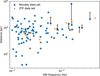 |
Fig. 1 GW frequency and distance of the binaries in the Munday and ZTF datasets. When a binary appears in both datasets, the two corresponding points are connected with a line; the distances differ due to the use of different distance measurement techniques. |
2.3 Correcting for observational biases
To compare the galaxy models to the observed DWDs, we accounted for the fact that the observed samples do not contain all Galactic DWDs, but only those that are both bright enough to be detected by EM telescopes and identifiable as binaries via eclipses or radial velocity measurements. Therefore, to get an indication of whether a model is overpredicting or underpredicting compared to reality, we needed to calculate how many of the DWDs predicted by the model would actually be detectable, for which an understanding of the observational biases is required.
A detailed modelling of all the relevant observational selection effects is highly complicated. However, given the very large discrepancy between the population synthesis models, we aimed to investigate some upper limits on the number of observable systems in the models and compare those to the real observed number.
Here we note some differences between our two observational datasets: the ZTF dataset mostly consists of DWDs detected through eclipses, while the Munday dataset includes both the DWDs detected through eclipses and ones detected through radial velocity measurements. Additionally, as stated in Sect. 2.2, the ZTF dataset is based on observations from a single telescope that has covered a significant fraction of the sky in a homogeneous way, while the Munday dataset uses multiple telescopes with inhomogeneous sky and parameter coverage. For these reasons, the observational biases affecting each dataset are different, and those of the ZTF dataset are simpler to calculate numerically, and so for the remainder of this section as well as for the corresponding results in Sect. 3.2, we only used the ZTF dataset.
2.3.1 Probability of eclipsing
The DWDs in the ZTF dataset have been identified as binaries through eclipses; that is, one of the WDs passing in front of the other from the perspective of the Earth, occluding its light and causing a dip in the light curve. There are two exceptions in the dataset, PTF J0533+0209 and ZTF J2320+3750 (Burdge et al. 2020b), which are not eclipsing but were identified as binaries through ellipsoidal variability in their light curves (see e.g. Morris 1985), though their inclinations are similar to those of the eclipsing systems in the sample of Burdge et al. (2020b).
Eclipses are only visible if the plane of the binary’s orbit is oriented in such a way that the WDs pass in front of each other from the perspective of the Earth. The range of orientations for which an eclipse occurs, and therefore the probability that a randomly oriented binary will be eclipsing, is proportional to P−2/3, where P is the orbital period of the binary (e.g. van Roestel et al. 2018; El-Badry et al. 2022); that is, short-period binaries are more likely to be eclipsing than longer-period binaries, introducing a period or frequency bias into the observations.
Specifically, from geometrical considerations one finds that a binary will be eclipsing from the perspective of the Earth if
![Mathematical equation: $\[\cos \iota<\frac{R_1+R_2}{a},\]$](/articles/aa/full_html/2025/07/aa54302-25/aa54302-25-eq1.png) (1)
(1)
where ι is the inclination of the binary’s orbital plane with respect to the Earth, a is the binary’s semi-major axis and R1 and R2 are the radii of the two binary components, respectively. If a binary is oriented randomly, then (R1 + R2)/a gives the probability that it is eclipsing.
The relation between a WD’s mass, which we know for the population synthesis models, and its radius is quite complex and non-linear. One commonly used formulation is given by Verbunt & Rappaport (1988) based upon calculations by Peter Eggleton:
![Mathematical equation: $\[\begin{aligned}R & =0.0114\left[\left(\frac{M}{M_{\mathrm{Ch}}}\right)^{-2 / 3}-\left(\frac{M}{M_{\mathrm{Ch}}}\right)^{2 / 3}\right]^{1 / 2} \\& \times\left[1+3.5\left(\frac{M}{M_p}\right)^{-2 / 3}+\left(\frac{M}{M_p}\right)^{-1}\right]^{-2 / 3}.\end{aligned}\]$](/articles/aa/full_html/2025/07/aa54302-25/aa54302-25-eq2.png) (2)
(2)
In this equation, R is the WD radius in R⊙, M is the WD mass in M⊙, MCh is the Chandrasekhar mass (1.44 M⊙) and Mp is a constant with a value of 5.7 × 10⁻⁴ M⊙.
We note that Parsons et al. (2017) found that the (zero-temperature) Verbunt & Rappaport (1988) mass-radius relation may underpredict WD radii, particularly for WDs with low masses and/or high temperatures. Similarly, when we compared the radii produced by Eq. (2) to the WD masses and radii actually measured in the ZTF dataset, we found that the radii predicted by Eq. (2) were generally smaller than those actually measured; this is illustrated in Fig. 2, where the points are those WDs from the ZTF dataset for which both a mass and a radius are listed, and the blue line shows the radii predicted by Eq. (2) for WD masses between 0.1 and 0.6 M⊙. We also plot, in the orange line, the radii from Eq. (2) multiplied by a factor of 3/2; by manual inspection, this line fits most of the ZTF WDs reasonably well, apart from a few outliers that we discuss in the next paragraph. Due to scatter and uncertainty in the ZTF mass-radius measurements, the ‘true’ coefficient could potentially be somewhat larger or smaller, though probably not by more than a factor of two, which is small compared to the order-of-magnitude differences between the population models. Hence, we judged that additional statistical analysis would not have significant benefit, and used a value of 3/2 for this coefficient. Therefore, we calculated the probability of a binary in the model populations eclipsing with Eq. (1), using the radii from Eq. (2) multiplied by 3/2. We use this eclipse probability to weight each object when we sum the total number of DWDs in a frequency-distance bin in Sect. 3.2.
There are some outliers in Fig. 2 with larger radii than predicted by our fit to the mass-radius relationship. However, we note that the two WDs with the largest radii in Fig. 2 are unusual objects. The largest WD belongs to the binary ZTF J2320+3750 and may be an extremely low-mass WD (Burdge et al. 2020b). The second-largest WD belongs to ZTF J0526+5934; as mentioned previously, it is not certain whether this object is actually a WD or a hot subdwarf (Kosakowski et al. 2023b; Lin et al. 2024), though Rebassa-Mansergas et al. (2024) argue that it is most likely to be a WD, just with a lower mass than in the ZTF data.
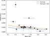 |
Fig. 2 Comparison between the WD radii predicted by Eq. (2) and those of the WDs in the ZTF DWD dataset with both mass and radius listed. The black points represent the observed WDs, with measurement uncertainties. The blue line shows the radii as predicted by Eq. (2), and the orange line shows those radii multiplied by 3/2. The two outliers with the largest radii might be extremely low-mass WDs (Burdge et al. 2020b), or could be hot subdwarfs instead of WDs (Kosakowski et al. 2023b; Lin et al. 2024; Rebassa-Mansergas et al. 2024). |
2.3.2 ZTF sky coverage
The ZTF survey is based upon the data from a single telescope facility, and so it does not cover the full sky. This reduces the probability of detecting a given DWD: even if it is eclipsing, it will not be detected if it is located in a part of the sky that ZTF cannot observe.
To estimate the probability that a given DWD is within ZTF’s sky coverage, we first note that 75% of the sky is visible from the Palomar telescope facility used by ZTF. The primary grid of ZTF pointings, used for ZTF’s DWD survey, covers approximately 88% of the sky visible from ZTF (Bellm et al. 2019b,a). This grid is divided into 636 fields, of which 598 have been observed at least 600 times, which is sufficient to be considered well-sampled for the purposes of detecting eclipsing DWDs (van Roestel et al. 2022). Thus, the fraction of the sky that is well-sampled by ZTF is ![Mathematical equation: $\[0.75 \times 0.88 \times \frac{598}{636} \approx 0.62\]$](/articles/aa/full_html/2025/07/aa54302-25/aa54302-25-eq3.png) .
.
The preceding calculation ignores that DWDs are not distributed isotropically through the sky, but are more concentrated in the Galactic disc. An alternative way of formulating the sky coverage is to take each of the WDs in the Gaia all-sky catalogue (Gentile Fusillo et al. 2021) and find how many times their sky location has been observed by ZTF. Then, the fraction of WDs that have been observed at least 600 times is approximately 0.54.
The difference between these two values is small compared to the orders-of-magnitude differences between the population synthesis models, so for simplicity we used a value of 0.6 for the ZTF sky coverage. We used this value for the detectability-corrected population synthesis predictions in Sect. 3.2: once we calculated the number of DWDs in the population synthesis models that would be eclipsing, we multiplied the total in each frequency bin by 0.6 to reflect the number of these that would be located within ZTF’s sky coverage.
2.3.3 ZTF magnitude limit
Aside from the eclipse probability and ZTF’s sky coverage, another factor that limits how many of the DWDs from the population synthesis models would actually be detectable is brightness. That is, ZTF can only detect binaries if they are sufficiently bright – specifically, if they are brighter than the limiting magnitude of the detector. For ZTF, the limiting magnitude is 21.1–20.8 in g-band and 20.9–20.6 in r-band (Bellm et al. 2019b); however, identifying the binarity of a DWD is more difficult than simply detecting light, and all of the DWDs in the ZTF dataset have a magnitude of 20.5 or brighter.
Taking into account that not all DWDs in the model population would be bright enough to be detectable would further lower the predicted numbers of detectable DWDs in the models. We investigated this by taking the SEBA galaxy model of Korol et al. (2017) and computed a new model population by only including those DWDs brighter than a certain threshold (for which we took an r-band magnitude of 20.5 as a default value).
The WD magnitudes were calculated within SEBA as described in Toonen & Nelemans (2013), using WD cooling models from Holberg & Bergeron (2006); Kowalski & Saumon (2006); Tremblay et al. (2011). We computed the WD absolute magnitudes as a function of WD cooling time and WD mass via interpolation in the cooling model tables. In this procedure, the WD radius is not explicitly used, so the adaptation of the WD radii that we use to calculate the eclipse probabilities does not affect the calculation of the magnitude. The question is whether the increase in radius we find observationally would have an influence on the cooling models, but this is beyond the scope of this paper. The effect on the magnitude as a function of cooling age is also not straightforward: a larger radius results in higher luminosity for a given effective temperature, but also leads to faster cooling, i.e. lower effective temperature and luminosity at a given age.
Galactic extinction was applied to the WD magnitudes using the model of Sandage (1972) as implemented in Nelemans et al. (2004). We added together the r-band magnitudes of the two components as follows, to compute a total magnitude which we compared to the threshold:
![Mathematical equation: $\[m_{\mathrm{tot}}=-2.5 ~\log \left(10^{\frac{m_1}{-2.5}}+10^{\frac{m_2}{-2.5}}\right).\]$](/articles/aa/full_html/2025/07/aa54302-25/aa54302-25-eq4.png) (3)
(3)
In this equation, m1 and m2 are the magnitudes of the two components and mtot is the combined magnitude.
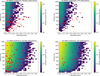 |
Fig. 3 Comparison of the BPASS (panels A and B) and SEBA (panels C and D) model populations to the observed systems from the Munday dataset (panels A and C) and the ZTF dataset (panels B and D), in terms of the GW frequency and distance of the binaries. Each rectangular cell represents a frequency-distance bin and is shaded according to the number of systems the population synthesis model predicts for that bin; white indicates that zero systems are predicted. Each red dot is an observed system. |
3 Results
3.1 DWDs by frequency and distance
The top two panels of Fig. 3 plot the DWDs present in the BPASS galaxy model in terms of the frequency and distance of the systems, compared to the observed systems from the Munday and ZTF datasets. The bottom panels show the same, but using the SEBA galaxy model.
By comparing these figures, it is immediately apparent that the SEBA galaxy model contains far more high-frequency DWDs than the BPASS galaxy model, affirming the conclusions of Tang et al. (2024) and van Zeist et al. (2024). For both galaxy models, the total number of DWDs in the model is orders of magnitude higher than the number of observed DWDs, but this is expected due to the limitations of the observations.
However, for the BPASS galaxy model, the top row of Fig. 3 indicates that at the highest frequencies (>10−3 Hz), the total number of predicted binaries is comparable to the number of observed binaries. However, as in this comparison we do not account for the selection effects that limit the EM observations, we would expect the number of predicted binaries to be significantly higher than the number of observed binaries (except possibly at the closest distances), as seen for the SEBA galaxy model in the bottom row of Fig. 3. This suggests the BPASS galaxy model may be underpredicting the number of high-frequency DWDs; we investigate this in more detail in the next sections.
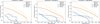 |
Fig. 4 Cumulative sum of the number of DWDs per frequency bin in the model populations compared to the observed population from ZTF, for several distance ranges. The cumulative sum is calculated for binaries in the frequency range of 10−4 to 10−2 Hz, starting at the high-frequency end. For the models, the dotted lines represent the total numbers of DWDs while the solid lines indicate the numbers of DWDs corrected to account for observational biases, providing an estimate of how many DWDs would be detectable in EM, though these are still upper limits. |
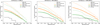 |
Fig. 5 Comparison of the full SEBA galaxy model and the SEBA population including only DWDs brighter than magnitude 20.5 (r-band) to the observed population from ZTF. The cumulative number of DWDs per frequency bin is plotted, as in Fig. 4. |
3.2 Model predictions of DWDs adjusted for observational biases
In Fig. 4, we compared the numbers of DWDs predicted in the two galaxy models to those in the observed ZTF dataset. Specifically, we plotted the cumulative sum of the number of DWDs per frequency bin in the frequency range of 10−4 to 10−2 Hz, starting from 0 at the high-frequency end. The different panels show the DWDs in different distance ranges – from 0 to 500 pc, from 500 pc to 1000 pc, and from 1000 to 2000 pc, respectively. For the model populations, the dotted lines indicate the total number of binaries present in the galaxy model. For the solid lines, we applied a correction by weighting each system according to its probability of being an eclipsing binary, using Eq. (1) as described in Sect. 2.3.1, and then multiplying the sum of each frequency bin by a factor related to ZTF’s sky coverage, as described in Sect. 2.3.2. This gives an upper limit to how many binaries in these models would actually be observed when taking into account that not all DWDs would be eclipsing and ZTF does not observe the whole sky. For the observational data, we only plotted the ZTF dataset here because, we stress again, the Munday dataset contains DWDs observed by multiple telescopes using various detection methods, and so the observational biases would be different and we could not compare the Munday data to the model populations specifically corrected for ZTF’s biases.
We can see that the corrected BPASS line lies below the line of the observed ZTF binaries at high frequencies, even though this corrected line still represents an upper limit on the numer of systems in the BPASS model population that would actually be detectable by ZTF. This trend is found in all of the distance bins, though the BPASS line is closer to the observed line for the farthest distance bin, which is to be expected as at greater distance other observational limits such as the telescope magnitude/luminosity limit become more relevant. This indicates that BPASS is clearly underpredicting the amount of high-frequency DWDs when compared to EM observations.
The corrected SEBA lines in Fig. 4 lie above the ZTF line for high-frequency DWDs. However, as noted above, this line is still an upper limit because the only observational biases accounted for are the probability of eclipsing and the limits of ZTF’s sky coverage. Therefore, we cannot conclude whether and to what degree SEBA might be overpredicting compared to the observations based on this alone. To investigate this further, we accounted for another limitation of the ZTF observations in Fig. 5: the telescope can only detect the DWDs if they are sufficiently bright, or specifically if they are brighter than the limiting magnitude of ZTF. For this, we took a value of 20.5 in the r-band as described in Sect. 2.3.3.
In Fig. 5 we plotted the numbers of DWDs for the total and eclipse/sky-coverage-corrected SEBA populations as in Fig. 4, along with a SEBA population which includes only DWDs brighter than magnitude 20.5, as described in Sect. 2.3.3. The solid green line includes both the eclipse and sky-coverage corrections and the magnitude limit. For the closest binaries, those within 500 pc, the magnitude limit only has a small effect on the predictions, and the SEBA predictions remain an order of magnitude above the ZTF observations. However, for DWDs between 500 and 1000 pc, the remaining difference is smaller. For the more distant DWDs between 1 and 2 kpc the magnitude-limited SEBA model is still above the ZTF line, but within a factor of a few at high frequencies.
Therefore, we can say that between 1 and 2 kpc the observability-corrected SEBA model population matches the observations, given the relatively simple assumptions we make in our models of the DWDs’ detectability. However, within 500 pc the SEBA galaxy model does appear to predict more DWDs than are observed in reality.
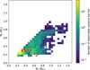 |
Fig. 6 Comparison of the component masses of the DWDs in the SEBA population with an r-band magnitude limit of 20.5 to the observed ZTF population. Each rectangular cell represents a mass bin and is shaded according to the number of systems SEBA predicts for that bin (corrected for the magnitude limit, the probability of eclipsing, and the ZTF sky coverage). Each red dot is an observed system. Here, we take M1 to always be the more massive of the WDs in the binary. |
3.3 Comparison of DWD mass distributions
In order to check for other possible selection effects in the data (e.g. based on the masses of the WDs), we plot in Fig. 6 the masses of the two WDs in each binary in the SEBA population (with an r-band magnitude limit of 20.5 and corrections for eclipsing probability and ZTF’s sky coverage applied) to those of the observed ZTF binaries. Only those DWDs in the ZTF dataset for which the masses of both components have been measured are included.
Despite the smaller ZTF sample size, the mass distributions of the predicted and observed populations resemble each other; no large fraction of the SEBA population is unrepresented in the ZTF population, or vice versa. However, the mass distributions of the SEBA predictions and the ZTF observations are not identical. Investigating the differences in more detail would require additional modelling of observational biases affecting the WD mass distribution, which is beyond the scope of this study.
4 Discussion
4.1 Implications for CEE models
Tang et al. (2024) and van Zeist et al. (2024) showed that the differences in the numbers of LISA-detectable DWDs between BPASS and other stellar evolution codes like SEBA and BSE are primarily caused by differences in the treatment of the stability of mass transfer and the modelling of CEEs. Firstly, mass transfer is more likely to be stable in BPASS than in other codes (Briel et al. 2023; van Zeist et al. 2024), resulting in the occurrence of fewer CEEs. Secondly, the method by which CEEs themselves are modelled in BPASS is qualitatively different.
Rapid population synthesis codes such as SEBA and BSE use analytic prescriptions to model the outcomes of CEEs, the most common being the α-formalism (Webbink 1984) and the γ-formalism (Nelemans et al. 2000; Nelemans & Tout 2005), though alternative prescriptions also exist, such as those of Trani et al. (2022) and Hirai & Mandel (2022). In BPASS, by contrast, the stellar structure is evolved in detail throughout the CEE (Eldridge et al. 2017; Stevance et al. 2023). However, the detailed CEE model of BPASS is still dependent on assumptions and simplifications about the physics of stellar interactions, and so its results are not necessarily more accurate or realistic.
In particular, CEEs in BPASS tend to be more efficient than in SEBA and BSE. This means that the binaries tend to lose less angular momentum during the CEE and thus undergo less orbital shrinkage (Stevance et al. 2023), resulting in wider orbits at the end of the CEE. Consequently, this reduces the number of DWDs emitting GWs in the LISA frequency band compared to other codes (Tang et al. 2024; van Zeist et al. 2024). When compared to α and γ-prescriptions, the effective αλ and γ parameters of the BPASS CEEs are much higher than those used in SEBA; for example, in BPASS the effective αλ value tends to be between 8 and 20 for CEE in the first binary interaction and between 4 and 30 for the second (van Zeist et al. 2024), while the SEBA version of Toonen et al. (2012) assumes αλ = 2, which means that the BPASS CEE model is an order of magnitude more efficient.
The SEBA values for αλ and γ were calculated based on fits to astrophysical observations of DWDs (Nelemans et al. 2000, 2001b), which raises the question of whether the much higher values from the BPASS CEE model are not representative in this case. Our results in this study, in which BPASS clearly underpredicts short-period DWDs compared to observations, suggest that the BPASS CEE model is indeed too efficient. However, we note that in this study we are only testing the CEE models for low- and intermediate-mass stars, as massive stars do not produce WDs. Furthermore, Briel et al. (2023) found that BPASS’s predictions for massive binaries do match the rates of BH binaries detected by LVK. Therefore, it is important to consider that modelling stars in different mass ranges may require different CEE prescriptions.
Additionally, these results show that LISA, which will identify a far larger number of Galactic DWDs than the EM surveys we used (Amaro-Seoane et al. 2023), will provide invaluable information on the processes of mass transfer and CEEs. This aligns with the results of Delfavero et al. (2025), who found that LISA’s future observations of the Galactic DWD population will be able to constrain CEE efficiency parameters to a level of about 10%.
4.2 Additional observational limiting factors
Our estimates of how many DWDs in the model populations would be detectable by ZTF through eclipses are upper limits, as there are additional factors which limit the detections of the DWDs and their eclipses. One of these relates to eclipse depth, which measures how much a DWD’s apparent brightness decreases during an eclipse. Eq. (1) gives the probability of an eclipse of any depth. However, ZTF can only identify an eclipse as such if the eclipse depth is at least approximately 10% of the total brightness (El-Badry et al. 2022). The eclipse depth is not trivial to calculate, as it depends on the luminosities and temperatures of the WDs, which in turn depend on modelling of WD cooling. The implication of the eclipse depth threshold is that the amount of DWDs in a population that ZTF could actually identify as eclipsing binaries would be slightly lower than the total numbers shown in Figs. 4 and 5.
Another limiting factor is that DWDs are not distributed isotropically across the sky, but are most likely to be found in the MW disc (e.g. Lamberts et al. 2019; Breivik et al. 2020b), which is where the sky density of stars is also highest. This high density results in crowding, where the close proximity of multiple different light sources makes it more difficult to resolve the light of each individual one (e.g. Scheuer 1957; Condon 1974; Renzini 1998; Olsen et al. 2003).
As a result, the threshold magnitude at which ZTF could detect DWDs would effectively be somewhat brighter than previously assumed for sources in the Galactic plane, which would lower the numbers of DWDs in the model populations that are bright enough to be detected by ZTF. In Fig. 7, we plotted what the magnitude-limited SEBA population from Sect. 2.3.3 and Fig. 5 looks like when we vary the magnitude limits between 21 and 19.5. We see that, for binaries closer than 500 pc, the SEBA predictions remain an order of magnitude above the ZTF observations, with a magnitude limit of 19.5 resulting in about half as many detectable DWDs than a limit of 20.5. However, for binaries between 500 and 1000 pc, the SEBA predictions match or even fall below the ZTF observations if the magnitude limit is 19.5 or brighter, at least at high frequencies, and for binaries between 1000 to 2000 pc this is the case for a magnitude limit of 20 or brighter.
While we use a default magnitude limit of 20.5, a limit of 20 is not unreasonable in the presence of crowding and extinction in the MW disc, where the largest concentration of DWDs reside. Therefore, the SEBA predictions are consistent with the ZTF observations of DWDs beyond 500 pc, but the SEBA model does appear to overpredict the number of observable DWDs within 500 pc by up to an order of magnitude. Because of the distance dependence, it is possible that the overprediction at low distances is caused by the spatial distribution of the MW model used by Korol et al. (2017), as opposed to the intrinsic stellar evolution modelling of SEBA.
Specifically, Korol et al. (2017) assumed a SFH from Boissier & Prantzos (1999) and an axisymmetric disc structure as detailed in Nelemans et al. (2004), where the stellar density is homogeneous for all points within the disc at a given distance from the Galactic centre, and so features such as spiral arms are not accounted for, which could have an effect on the density of DWDs close to the Earth. In particular, part of the Perseus Arm is within 2 kpc of Earth (Xu et al. 2006), which could contribute to the number of DWDs in the distance bin between 1 and 2 kpc but not to the nearer bins.
However, Tang et al. (2024) used a non-axisymmetric model for the structure of the MW disc, and they found that if they varied the location of the Earth between different points at the same Galactic radius, the changes in the WD density were small, with the amount of LISA-detectable DWDs varying by only a few percent. Therefore, it is not clear whether Korol et al. (2017)’s assumption of axisymmetry would have a large effect on the local density of DWDs. There are also other differences between the MW models used by Korol et al. (2017) and Tang et al. (2024) that could affect the local stellar density, such as the disc scale parameters, which determine the thickness and distribution of the disc. However, a detailed examination of these MW structure models is beyond the scope of this paper.
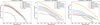 |
Fig. 7 Comparison of the SEBA galaxy model, including only DWDs brighter than various (r-band) magnitude limits, with the observed population from ZTF. The cumulative number of DWDs per frequency bin is plotted, as in Fig. 4. All lines are corrected for eclipsing probability and ZTF’s sky coverage. |
4.3 Uncertainties in population synthesis predictions
There are some uncertainties in the process by which we translate the BPASS and SEBA galaxy models into predictions of EM-detectable DWDs. Firstly, the WD radii we calculate in Sect. 2.3.1 are approximate and based on a fit to the manual radii in the ZTF dataset; as can be seen in Fig. 2, there are a few ZTF WDs that are outliers with respect to the mass-radius relationship, and there generally is a degree of scatter in the ZTF measurements, which creates uncertainty in the mass-radius relationship. This, in turn, creates uncertainty in the eclipse probabilities for each of the model systems.
Secondly, as noted in Sect. 2.3.3, the WD magnitudes from SEBA were computed using cooling models that do not necessarily have radii consistent with those we used to calculate the probability of a DWD being eclipsing. Given the counterbalancing effects of larger radii leading to brighter WDs but also to faster cooling, we believe that the effect of the larger radii is (much) less important for the magnitude cuts than for the eclipse probability.
Another source of uncertainty is the cooling models themselves, as these assume that all WDs have a carbon–oxygen (CO) chemical composition (Toonen & Nelemans 2013). Thus, for WDs with masses below approximately 0.5 M⊙ or above 1.1 M⊙, which would be expected to have different chemical compositions in reality, the calculated luminosities are less accurate.
4.4 Using the Munday dataset as a magnitude-limited sample
When we compared the frequency distributions of the DWDs in the population synthesis models to those in the EM observations, we only used the systems in the ZTF dataset because, as previously mentioned, the Munday dataset contains observations from multiple different telescopes, and from both eclipsing DWDs and DWDs detected through radial velocity measurements. The latter category makes up a majority of the Munday DWDs, particularly at frequencies lower than 10−3 Hz.
DWDs detected through radial velocity measurements usually have g-band magnitudes of 18 or brighter (see e.g. Munday et al. 2024). One may wonder if it is possible to use the Munday dataset as a complete magnitude-limited sample in a comparison with the population synthesis models. However, the Munday dataset contains only 41 DWDs with a g-band magnitude of 18 or brighter, a GW frequency of 10−4 Hz or higher, and a distance of no more than 1 kpc from Earth. By comparison, the SEBA galaxy model contains 791 such DWDs. Similarly, using a g-band magnitude limit of 16, the Munday dataset has 15 DWDs, while the SEBA galaxy model has 96.
This indicates that the Munday dataset is quite incomplete in terms of capturing the full population of DWDs brighter than a certain threshold. Therefore, while the Munday dataset is highly interesting in terms of learning about properties of DWDs, we cannot use it for evaluating the total number or space density of DWDs, which is the aim of this paper.
5 Conclusions
We took the DWDs predicted by the BPASS galaxy model of Tang et al. (2024) and the SEBA galaxy model of Korol et al. (2017), and compared them to the DWDs observed by EM surveys. Compared to the observations, we find that the BPASS model underpredicts short-period (high-frequency) DWDs by a factor of at least ten. By contrast, the SEBA model is roughly consistent with the DWD observations for systems between 500 pc and 1 kpc, and clearly consistent for those beyond 1 kpc. However, it may overpredict the number of DWDs within 500 pc, though by no more than a factor of ten. Due to the uncertainties in the selection effects, we cannot make a more definitive statement about the SEBA model.
These results imply that the total number of resolved LISA DWDs will likely be of the order of 10 000, as opposed to fewer than 1000 as predicted by Tang et al. (2024). There may be additional selection effects that we have not modelled, which would decrease the DWD rates predicted by the population synthesis models compared to the observations. This would increase the factor by which the BPASS model underpredicts and decrease the factor by which the SEBA model may be overpredicting.
As the treatment of mass transfer and CEEs in BPASS compared to SEBA is the main factor causing the difference in the predictions of short-period, LISA-detectable DWDs between these codes (van Zeist et al. 2024), this study provides a valuable test of common-envelope prescriptions. It shows that the BPASS CEE prescription is too efficient for low- and intermediate-mass stars. As earlier research by Briel et al. (2023) found that BPASS predictions are consistent with GW observations for massive (BH-forming) stars, these findings together indicate that modelling stars in different mass ranges may require different CEE prescriptions. Additionally, our findings highlight how LISA’s observations of DWDs will provide invaluable information on mass transfer and CEEs.
Data availability
The BPASS models can be downloaded from https://bpass.auckland.ac.nz. The Munday et al. (2024) observed DWD catalogue can be downloaded from https://github.com/JamesMunday98/CloseDWDbinaries. Other data underlying this article will be shared upon reasonable request to the corresponding author.
Acknowledgements
The authors thank the anonymous referee for their comments, and Paul J. Groot, James Munday and Simon F. Portegies Zwart for useful discussions. WGJvZ acknowledges support from Radboud University, the European Research Council (ERC) under the European Union’s Horizon 2020 research and innovation programme (grant agreement No. 725246), Dutch Research Council grant 639.043.514 and the University of Auckland. JJE acknowledges support from Marsden Fund Council grant MFP-UOA2131 managed through the Royal Society of New Zealand Te Apārangi.
References
- Abbott, R., Abbott, T. D., Acernese, F., et al. 2023, Phys. Rev. X, 13, 041039 [Google Scholar]
- Abt, H. A. 1983, ARA&A, 21, 343 [Google Scholar]
- Amaro-Seoane, P., Andrews, J., Arca Sedda, M., et al. 2023, Liv. Rev. Relativ., 26, 2 [NASA ADS] [CrossRef] [Google Scholar]
- Amaro-Seoane, P., Audley, H., Babak, S., et al. 2017, arXiv e-prints, [arXiv:1702.00786] [Google Scholar]
- Antunes Amaral, L., Munday, J., Vučković, M., et al. 2024, A&A, 685, A9 [NASA ADS] [CrossRef] [EDP Sciences] [Google Scholar]
- Bailer-Jones, C. A. L., Rybizki, J., Fouesneau, M., Demleitner, M., & Andrae, R. 2021, AJ, 161, 147 [Google Scholar]
- Belczynski, K., Kalogera, V., & Bulik, T. 2002, ApJ, 572, 407 [NASA ADS] [CrossRef] [Google Scholar]
- Belczynski, K., Kalogera, V., Rasio, F. A., et al. 2008, ApJS, 174, 223 [Google Scholar]
- Bellm, E. C., Kulkarni, S. R., Barlow, T., et al. 2019a, PASP, 131, 068003 [Google Scholar]
- Bellm, E. C., Kulkarni, S. R., Graham, M. J., et al. 2019b, PASP, 131, 018002 [Google Scholar]
- Boissier, S., & Prantzos, N. 1999, MNRAS, 307, 857 [NASA ADS] [CrossRef] [Google Scholar]
- Bours, M. C. P., Marsh, T. R., Parsons, S. G., et al. 2014, MNRAS, 438, 3399 [NASA ADS] [CrossRef] [Google Scholar]
- Breivik, K. 2025, arXiv e-prints, [arXiv:2502.03523] [Google Scholar]
- Breivik, K., Coughlin, S., Zevin, M., et al. 2020a, ApJ, 898, 71 [Google Scholar]
- Breivik, K., Mingarelli, C. M. F., & Larson, S. L. 2020b, ApJ, 901, 4 [NASA ADS] [CrossRef] [Google Scholar]
- Briel, M. M., Stevance, H. F., & Eldridge, J. J. 2023, MNRAS, 520, 5724 [Google Scholar]
- Brown, W. R., Kilic, M., Allende Prieto, C., & Kenyon, S. J. 2010, ApJ, 723, 1072 [Google Scholar]
- Brown, W. R., Kilic, M., Hermes, J. J., et al. 2011, ApJ, 737, L23 [NASA ADS] [CrossRef] [Google Scholar]
- Brown, W. R., Kilic, M., Kosakowski, A., & Gianninas, A. 2017, ApJ, 847, 10 [NASA ADS] [CrossRef] [Google Scholar]
- Brown, W. R., Kilic, M., Kosakowski, A., et al. 2020, ApJ, 889, 49 [Google Scholar]
- Brown, W. R., Kilic, M., Kosakowski, A., & Gianninas, A. 2022, ApJ, 933, 94 [NASA ADS] [CrossRef] [Google Scholar]
- Burdge, K. B., Coughlin, M. W., Fuller, J., et al. 2020a, ApJ, 905, L7 [NASA ADS] [CrossRef] [Google Scholar]
- Burdge, K. B., Coughlin, M. W., Fuller, J., et al. 2019, Nature, 571, 528 [Google Scholar]
- Burdge, K. B., Prince, T. A., Fuller, J., et al. 2020b, ApJ, 905, 32 [Google Scholar]
- Chakraborty, J., Burdge, K. B., Rappaport, S. A., et al. 2024, ApJ, 977, 262 [Google Scholar]
- Colpi, M., Danzmann, K., Hewitson, M., et al. 2024, arXiv e-prints, [arXiv:2402.07571] [Google Scholar]
- Condon, J. J. 1974, ApJ, 188, 279 [Google Scholar]
- Coughlin, M. W., Burdge, K., Phinney, E. S., et al. 2020, MNRAS, 494, L91 [NASA ADS] [CrossRef] [Google Scholar]
- Delfavero, V., Breivik, K., Thiele, S., O’Shaughnessy, R., & Baker, J. G. 2025, ApJ, 981, 66 [Google Scholar]
- El-Badry, K., Conroy, C., Fuller, J., et al. 2022, MNRAS, 517, 4916 [NASA ADS] [CrossRef] [Google Scholar]
- Eldridge, J. J., Stanway, E. R., Xiao, L., et al. 2017, PASA, 34, e058 [Google Scholar]
- Gaia Collaboration, Vallenari, A., Brown, A. G. A., et al. 2023, A&A, 674, A1 [NASA ADS] [CrossRef] [EDP Sciences] [Google Scholar]
- Gentile Fusillo, N. P., Tremblay, P. E., Cukanovaite, E., et al. 2021, MNRAS, 508, 3877 [NASA ADS] [CrossRef] [Google Scholar]
- Ghodla, S., van Zeist, W. G. J., Eldridge, J. J., Stevance, H. F., & Stanway, E. R. 2022, MNRAS, 511, 1201 [NASA ADS] [CrossRef] [Google Scholar]
- Hallakoun, N., Maoz, D., Kilic, M., et al. 2016, MNRAS, 458, 845 [NASA ADS] [CrossRef] [Google Scholar]
- Heggie, D. C. 1975, MNRAS, 173, 729 [NASA ADS] [CrossRef] [Google Scholar]
- Hils, D., Bender, P. L., & Webbink, R. F. 1990, ApJ, 360, 75, [CrossRef] [Google Scholar]
- Hirai, R., & Mandel, I. 2022, ApJ, 937, L42 [NASA ADS] [CrossRef] [Google Scholar]
- Holberg, J. B., & Bergeron, P. 2006, AJ, 132, 1221 [Google Scholar]
- Holberg, J. B., Oswalt, T. D., Sion, E. M., & McCook, G. P. 2016, MNRAS, 462, 2295 [NASA ADS] [CrossRef] [Google Scholar]
- Hopkins, P. F., Kereš, D., Oñorbe, J., et al. 2014, MNRAS, 445, 581 [NASA ADS] [CrossRef] [Google Scholar]
- Hurley, J. R., Tout, C. A., & Pols, O. R. 2002, MNRAS, 329, 897 [Google Scholar]
- Keim, M. A., Korol, V., & Rossi, E. M. 2023, MNRAS, 521, 1088 [NASA ADS] [CrossRef] [Google Scholar]
- Keller, P. M., Breedt, E., Hodgkin, S., et al. 2022, MNRAS, 509, 4171 [Google Scholar]
- Kilic, M., Brown, W. R., Allende Prieto, C., et al. 2011, ApJ, 727, 3 [Google Scholar]
- Kilic, M., Hermes, J. J., Gianninas, A., et al. 2014, MNRAS, 438, L26 [NASA ADS] [CrossRef] [Google Scholar]
- Koester, D., Napiwotzki, R., Christlieb, N., et al. 2001, A&A, 378, 556 [NASA ADS] [CrossRef] [EDP Sciences] [Google Scholar]
- Korol, V., Rossi, E. M., Groot, P. J., et al. 2017, MNRAS, 470, 1894 [NASA ADS] [CrossRef] [Google Scholar]
- Korol, V., Hallakoun, N., Toonen, S., & Karnesis, N. 2022, MNRAS, 511, 5936 [NASA ADS] [CrossRef] [Google Scholar]
- Kosakowski, A., Brown, W. R., Kilic, M., et al. 2023a, ApJ, 950, 141 [CrossRef] [Google Scholar]
- Kosakowski, A., Kupfer, T., Bergeron, P., & Littenberg, T. B. 2023b, ApJ, 959, 114 [NASA ADS] [CrossRef] [Google Scholar]
- Kowalski, P. M., & Saumon, D. 2006, ApJ, 651, L137 [Google Scholar]
- Królak, A., Tinto, M., & Vallisneri, M. 2004, Phys. Rev. D, 70, 022003 [Google Scholar]
- Kroupa, P., Tout, C. A., & Gilmore, G. 1993, MNRAS, 262, 545 [NASA ADS] [CrossRef] [Google Scholar]
- Kruckow, M. U., Neunteufel, P. G., Di Stefano, R., Gao, Y., & Kobayashi, C. 2021, ApJ, 920, 86 [NASA ADS] [CrossRef] [Google Scholar]
- Kupfer, T., Korol, V., Littenberg, T. B., et al. 2024, ApJ, 963, 100 [NASA ADS] [CrossRef] [Google Scholar]
- Lamberts, A., Blunt, S., Littenberg, T. B., et al. 2019, MNRAS, 490, 5888 [NASA ADS] [CrossRef] [Google Scholar]
- Li, Z., Chen, X., Chen, H.-L., et al. 2020, ApJ, 893, 2 [NASA ADS] [CrossRef] [Google Scholar]
- Li, Z., Chen, X., Ge, H., Chen, H.-L., & Han, Z. 2023, A&A, 669, A82 [NASA ADS] [CrossRef] [EDP Sciences] [Google Scholar]
- Lin, J., Wu, C., Xiong, H., et al. 2024, Nat. Astron., 8, 491 [Google Scholar]
- Maoz, D., Badenes, C., & Bickerton, S. J. 2012, ApJ, 751, 143 [NASA ADS] [CrossRef] [Google Scholar]
- Maoz, D., Hallakoun, N., & Badenes, C. 2018, MNRAS, 476, 2584 [NASA ADS] [CrossRef] [Google Scholar]
- Marsh, T. R., Dhillon, V. S., & Duck, S. R. 1995, MNRAS, 275, 828 [Google Scholar]
- Moe, M., & Di Stefano, R. 2017, ApJS, 230, 15 [Google Scholar]
- Morris, S. L. 1985, ApJ, 295, 143 [Google Scholar]
- Munday, J., Tremblay, P. E., Hermes, J. J., et al. 2023, MNRAS, 525, 1814 [NASA ADS] [CrossRef] [Google Scholar]
- Munday, J., Pelisoli, I., Tremblay, P. E., et al. 2024, MNRAS, 532, 2534 [NASA ADS] [CrossRef] [Google Scholar]
- Napiwotzki, R., Christlieb, N., Drechsel, H., et al. 2001, Astron. Nachr., 322, 411 [NASA ADS] [CrossRef] [Google Scholar]
- Nelemans, G., & Tout, C. A. 2005, MNRAS, 356, 753 [NASA ADS] [CrossRef] [Google Scholar]
- Nelemans, G., Verbunt, F., Yungelson, L. R., & Portegies Zwart, S. F. 2000, A&A, 360, 1011 [NASA ADS] [Google Scholar]
- Nelemans, G., Yungelson, L. R., & Portegies Zwart, S. F. 2001a, A&A, 375, 890 [NASA ADS] [CrossRef] [EDP Sciences] [Google Scholar]
- Nelemans, G., Yungelson, L. R., Portegies Zwart, S. F., & Verbunt, F. 2001b, A&A, 365, 491 [NASA ADS] [CrossRef] [EDP Sciences] [Google Scholar]
- Nelemans, G., Yungelson, L. R., & Portegies Zwart, S. F. 2004, MNRAS, 349, 181 [NASA ADS] [CrossRef] [Google Scholar]
- Nissanke, S., Vallisneri, M., Nelemans, G., & Prince, T. A. 2012, ApJ, 758, 131 [NASA ADS] [CrossRef] [Google Scholar]
- O’Brien, M. W., Tremblay, P. E., Klein, B. L., et al. 2024, MNRAS, 527, 8687 [Google Scholar]
- Olsen, K. A. G., Blum, R. D., & Rigaut, F. 2003, AJ, 126, 452 [Google Scholar]
- Parsons, S. G., Marsh, T. R., Gänsicke, B. T., Drake, A. J., & Koester, D. 2011, ApJ, 735, L30 [NASA ADS] [CrossRef] [Google Scholar]
- Parsons, S. G., Gänsicke, B. T., Marsh, T. R., et al. 2017, MNRAS, 470, 4473 [Google Scholar]
- Portegies Zwart, S. F., & Verbunt, F. 1996, A&A, 309, 179 [NASA ADS] [Google Scholar]
- Rebassa-Mansergas, A., Hollands, M., Parsons, S. G., et al. 2024, A&A, 686, A221 [NASA ADS] [CrossRef] [EDP Sciences] [Google Scholar]
- Renzini, A. 1998, AJ, 115, 2459 [Google Scholar]
- Robinson, E. L., & Shafter, A. W. 1987, ApJ, 322, 296 [CrossRef] [Google Scholar]
- Ruiter, A. J., Belczynski, K., Benacquista, M., Larson, S. L., & Williams, G. 2010, ApJ, 717, 1006 [NASA ADS] [CrossRef] [Google Scholar]
- Sandage, A. 1972, ApJ, 178, 1 [Google Scholar]
- Scheuer, P. A. G. 1957, Proc. Cambr. Philos. Soc., 53, 764 [Google Scholar]
- Schneider, R., Ferrari, V., Matarrese, S., & Portegies Zwart, S. F. 2001, MNRAS, 324, 797 [NASA ADS] [CrossRef] [Google Scholar]
- Stanway, E. R., & Eldridge, J. J. 2018, MNRAS, 479, 75 [NASA ADS] [CrossRef] [Google Scholar]
- Steinfadt, J. D. R., Kaplan, D. L., Shporer, A., Bildsten, L., & Howell, S. B. 2010, ApJ, 716, L146 [NASA ADS] [CrossRef] [Google Scholar]
- Stevance, H. F., Eldridge, J. J., Stanway, E. R., et al. 2023, Nat. Astron., 7, 444 [NASA ADS] [CrossRef] [Google Scholar]
- Tang, P., Eldridge, J. J., Meyer, R., et al. 2024, MNRAS, 534, 1707 [NASA ADS] [CrossRef] [Google Scholar]
- Toonen, S., & Nelemans, G. 2013, A&A, 557, A87 [NASA ADS] [CrossRef] [EDP Sciences] [Google Scholar]
- Toonen, S., Nelemans, G., & Portegies Zwart, S. 2012, A&A, 546, A70 [NASA ADS] [CrossRef] [EDP Sciences] [Google Scholar]
- Toonen, S., Hollands, M., Gänsicke, B. T., & Boekholt, T. 2017, A&A, 602, A16 [NASA ADS] [CrossRef] [EDP Sciences] [Google Scholar]
- Trani, A. A., Rieder, S., Tanikawa, A., et al. 2022, Phys. Rev. D, 106, 043014 [NASA ADS] [CrossRef] [Google Scholar]
- Tremblay, P. E., Bergeron, P., & Gianninas, A. 2011, ApJ, 730, 128 [Google Scholar]
- van Roestel, J., Kupfer, T., Ruiz-Carmona, R., et al. 2018, MNRAS, 475, 2560 [CrossRef] [Google Scholar]
- van Roestel, J., Kupfer, T., Green, M. J., et al. 2022, MNRAS, 512, 5440 [NASA ADS] [CrossRef] [Google Scholar]
- van Roestel, J., Burdge, K., Caiazzo, I., et al. 2025, arXiv e-prints, [arXiv:2505.15580] [Google Scholar]
- van Zeist, W. G. J., Eldridge, J. J., & Tang, P. N. 2023, MNRAS, 524, 2836 [NASA ADS] [CrossRef] [Google Scholar]
- van Zeist, W. G. J., Nelemans, G., Portegies Zwart, S. F., & Eldridge, J. J. 2024, A&A, 691, A316 [NASA ADS] [CrossRef] [EDP Sciences] [Google Scholar]
- Verbunt, F., & Rappaport, S. 1988, ApJ, 332, 193 [NASA ADS] [CrossRef] [Google Scholar]
- Webbink, R. F. 1984, ApJ, 277, 355 [NASA ADS] [CrossRef] [Google Scholar]
- Wetzel, A., Hayward, C. C., Sanderson, R. E., et al. 2023, ApJS, 265, 44 [NASA ADS] [CrossRef] [Google Scholar]
- Xu, Y., Reid, M. J., Zheng, X. W., & Menten, K. M. 2006, Science, 311, 54 [NASA ADS] [CrossRef] [Google Scholar]
All Tables
All Figures
|
Fig. 1 GW frequency and distance of the binaries in the Munday and ZTF datasets. When a binary appears in both datasets, the two corresponding points are connected with a line; the distances differ due to the use of different distance measurement techniques. |
| In the text | |
|
Fig. 2 Comparison between the WD radii predicted by Eq. (2) and those of the WDs in the ZTF DWD dataset with both mass and radius listed. The black points represent the observed WDs, with measurement uncertainties. The blue line shows the radii as predicted by Eq. (2), and the orange line shows those radii multiplied by 3/2. The two outliers with the largest radii might be extremely low-mass WDs (Burdge et al. 2020b), or could be hot subdwarfs instead of WDs (Kosakowski et al. 2023b; Lin et al. 2024; Rebassa-Mansergas et al. 2024). |
| In the text | |
|
Fig. 3 Comparison of the BPASS (panels A and B) and SEBA (panels C and D) model populations to the observed systems from the Munday dataset (panels A and C) and the ZTF dataset (panels B and D), in terms of the GW frequency and distance of the binaries. Each rectangular cell represents a frequency-distance bin and is shaded according to the number of systems the population synthesis model predicts for that bin; white indicates that zero systems are predicted. Each red dot is an observed system. |
| In the text | |
|
Fig. 4 Cumulative sum of the number of DWDs per frequency bin in the model populations compared to the observed population from ZTF, for several distance ranges. The cumulative sum is calculated for binaries in the frequency range of 10−4 to 10−2 Hz, starting at the high-frequency end. For the models, the dotted lines represent the total numbers of DWDs while the solid lines indicate the numbers of DWDs corrected to account for observational biases, providing an estimate of how many DWDs would be detectable in EM, though these are still upper limits. |
| In the text | |
|
Fig. 5 Comparison of the full SEBA galaxy model and the SEBA population including only DWDs brighter than magnitude 20.5 (r-band) to the observed population from ZTF. The cumulative number of DWDs per frequency bin is plotted, as in Fig. 4. |
| In the text | |
|
Fig. 6 Comparison of the component masses of the DWDs in the SEBA population with an r-band magnitude limit of 20.5 to the observed ZTF population. Each rectangular cell represents a mass bin and is shaded according to the number of systems SEBA predicts for that bin (corrected for the magnitude limit, the probability of eclipsing, and the ZTF sky coverage). Each red dot is an observed system. Here, we take M1 to always be the more massive of the WDs in the binary. |
| In the text | |
|
Fig. 7 Comparison of the SEBA galaxy model, including only DWDs brighter than various (r-band) magnitude limits, with the observed population from ZTF. The cumulative number of DWDs per frequency bin is plotted, as in Fig. 4. All lines are corrected for eclipsing probability and ZTF’s sky coverage. |
| In the text | |
Current usage metrics show cumulative count of Article Views (full-text article views including HTML views, PDF and ePub downloads, according to the available data) and Abstracts Views on Vision4Press platform.
Data correspond to usage on the plateform after 2015. The current usage metrics is available 48-96 hours after online publication and is updated daily on week days.
Initial download of the metrics may take a while.