| Issue |
A&A
Volume 691, November 2024
|
|
|---|---|---|
| Article Number | A316 | |
| Number of page(s) | 10 | |
| Section | Galactic structure, stellar clusters and populations | |
| DOI | https://doi.org/10.1051/0004-6361/202451026 | |
| Published online | 22 November 2024 | |
Evaluating the gravitational wave detectability of globular clusters and the Magellanic Clouds for LISA
1
Department of Astrophysics/IMAPP, Radboud University,
PO Box 9010,
6500
GL,
Nijmegen,
The Netherlands
2
Leiden Observatory, Leiden University,
Einsteinweg 55,
2333
CC,
Leiden,
The Netherlands
3
Department of Physics, University of Auckland,
Private Bag
92019
Auckland,
New Zealand
4
SRON, Netherlands Institute for Space Research,
Niels Bohrweg 4,
2333
CA
Leiden,
The Netherlands
5
Institute of Astronomy, KU Leuven,
Celestijnenlaan 200D,
3001
Leuven,
Belgium
★ Corresponding author; This email address is being protected from spambots. You need JavaScript enabled to view it.
Received:
7
June
2024
Accepted:
17
October
2024
Abstract
We used the stellar evolution code BPASS and the gravitational wave (GW) simulation code LEGWORK to simulate populations of compact binaries that may be detected by the future space-based GW detector LISA. Specifically, we simulate the Magellanic Clouds and binary populations mimicking several globular clusters, neglecting dynamical effects. We find that a handful of sources should be detectable in each of the Magellanic Clouds, but for globular clusters the amount of detectable sources will likely be less than one each. We compared our results to earlier research and find that our predicted numbers are several dozen times lower than both the results from calculations that used the stellar evolution code BSE and take dynamical effects into account, and results from calculations that used the stellar evolution code SEBA for the Magellanic Clouds. Earlier research that compared BPASS models for GW sources in the Galactic disk with BSE models found a similarly sized discrepancy. We determine that this discrepancy is caused by differences between the stellar evolution codes, particularly in the treatment of mass transfer and common-envelope events in binaries: in BPASS mass transfer is more likely to be stable and tends to lead to less orbital shrinkage in the common-envelope phase than in other codes. This difference results in fewer compact binaries with periods short enough to be detected by LISA existing in the BPASS population. For globular clusters, we conclude that the impact of dynamical effects is uncertain based on the literature, but the differences in stellar evolution have an effect of a factor of 20 to 40 on the number of detectable binaries.
Key words: gravitational waves / binaries: close / stars: neutron / white dwarfs / globular clusters: general / Magellanic Clouds
© The Authors 2024
 Open Access article, published by EDP Sciences, under the terms of the Creative Commons Attribution License (https://creativecommons.org/licenses/by/4.0), which permits unrestricted use, distribution, and reproduction in any medium, provided the original work is properly cited.
This article is published in open access under the Subscribe to Open model. This email address is being protected from spambots. You need JavaScript enabled to view it. to support open access publication.
1 Introduction
The Laser Interferometer Space Antenna (LISA; Amaro-Seoane et al. 2017; Colpi et al. 2024), a space-based astronomical observatory that is currently under development, is designed to detect gravitational waves (GWs) in a lower frequency band than those currently being detected by the ground-based LIGO–Virgo–KAGRA (LVK) Collaboration (Abbott et al. 2023). It will consist of three satellites in a triangular formation with a separation of 2.5 million km, which will rotate about their barycentre, and the barycentre will follow Earth’s orbit but trail it by approximately 20 degrees (see Cornish & Robson 2017).
According to predictions, LISA will be able to detect many different types of GW sources, ranging from those of astrophysical origin such as merging binary systems (Amaro-Seoane et al. 2023) to those of cosmological origin such as cosmic strings and inflation (Auclair et al. 2023). Unlike the LVK Collaboration detectors, which have not detected more than one GW signal at a time, LISA is expected to continuously receive multiple overlapping signals, and disentangling them will be a complex process (Littenberg et al. 2020).
To understand the signals that LISA will receive, it is beneficial to understand and model the different types of sources that LISA might detect, and the existing populations of these sources. One class of astrophysical sources for LISA are compact binaries of stellar origin. They are binary systems consisting mostly of two compact objects: black holes (BHs), neutron stars (NSs) and/or white dwarfs (WDs). Such binaries exist and can be detected in GWs: the GW signals that the LVK Collaboration have observed (catalogued most recently in Abbott et al. 2023) have been from the mergers of such binaries. LISA, having a lower frequency band, would detect such systems earlier in their evolution, when they are still at greater separations. Further evidence of the types of binaries that LISA will detect is given by the LISA verification binaries (catalogued most recently in Kupfer et al. 2024), a set of Galactic binaries known from electromagnetic (EM) observations; these binaries predominantly contain WDs, which, based on their frequencies and distances, would potentially be detectable by LISA.
There have been many studies about the populations of stellar compact binaries that LISA may detect (e.g. Paczyński 1967; Lipunov et al. 1987; Hils et al. 1990; Schneider et al. 2001; Nelemans et al. 2001a; Ruiter et al. 2010; Belczynski et al. 2010; Nissanke et al. 2012; Korol et al. 2017; Lamberts et al. 2018, 2019; Breivik et al. 2020b; Lau et al. 2020); an overview is given in Sect. 1 of Amaro-Seoane et al. (2023). The most numerous are expected to be WD–WD binaries in the Galactic disk.
We previously investigated the LISA binary sources in a generic, averaged stellar population in van Zeist et al. (2023). In the current paper, we focus on two different kinds of real, localised stellar populations that exist close to the Galaxy: globular clusters (GCs) and the Magellanic Clouds. The reason for this is that, if they contain LISA-detectable binaries, the detector could potentially resolve these localised populations on the sky against the background of the Galactic disk. LISA could then provide insights into the binary population that would not be possible with EM observations alone, for example by resolving binaries too faint to be detected in EM. We note that both GCs (e.g. Benacquista et al. 2001; Ivanova et al. 2006; Kremer et al. 2018) and the Magellanic Clouds (Roebber et al. 2020; Korol et al. 2020; Keim et al. 2023) have previously been considered as potential hosts of GW sources for LISA.
Globular clusters and the Magellanic Clouds differ in a number of ways, one of which is size: the Magellanic Clouds, being dwarf galaxies, are several orders of magnitude more massive than even the largest GCs. A subtler distinction is found in the composition and history of the stellar populations they contain: GCs are typically considered to be the result of a single cloud of gas collapsing, resulting in a burst of star formation that creates a population of stars that all have the same age and metallicity. However, this traditional view has been challenged by observations that show that some GCs contain multiple sub-populations with distinct chemical compositions; this phenomenon has been theorised to be the result of either some stars in the GCs being polluted by the material ejected from others, or this ejected material coalescing to form a new generation of stars (for an overview, see Bastian & Lardo 2018; Milone & Marino 2022, and references therein).
By contrast, the Magellanic Clouds contain stars of various ages and compositions, produced over an extended period of star formation. We note that despite the existence of multiple populations within individual GCs, GCs are still far more homogeneous than the Magellanic Clouds. For this study, we treated GCs as consisting of a single population, but took the star formation history (SFH) of the Magellanic Clouds into account using the models of Harris & Zaritsky (2004); Harris & Zaritsky (2009); this is described in more detail in Sect. 2.
Another relevant distinction between these two types of populations is that the Magellanic Clouds have a relatively low stellar density, similar to that of the Galactic disk, so we can treat their binaries as evolving in isolation (i.e. without external effects influencing the evolution). The GCs have a higher stellar density and correspondingly a lower average distance between stars. As a consequence, the chance that a stellar system will have a gravitational encounter with another system, wherein the orbits of the systems are affected or stars are even exchanged, is not negligible. These effects are known collectively as dynamical interactions (see e.g. Heggie 1975; Heggie & Hut 2003; Benacquista & Downing 2013; Kremer et al. 2020); we discuss the effects that dynamical interactions can have on the population of GW sources in a GC in detail in Sect. 4.2.
We did not simulate dynamical interactions in this study. Since it is not clear from earlier results how strongly dynamical interactions will increase or decrease the number of LISAdetectable binaries in a GC, particularly for WD binaries (the most numerous GW sources in the LISA band), we consider that studying the GW sources from an isolated binary population still provides a worthwhile comparison. Furthermore, performing these simulations with isolated binaries and then comparing our results to those found using other codes that do include dynamical interactions gives us an indication of the impact dynamical interactions have on the binary population.
This paper is structured as follows: in Sect. 2 we present our methods for modelling the GW sources in GCs and the Magellanic Clouds, in Sect. 3 we present our results, in Sect. 4 we discuss our results and compare them to those of similar studies in the literature and in Sect. 5 we summarise our conclusions.
2 Method
2.1 Modelling stellar populations with BPASS
To simulate the stellar populations that we drew GW sources from, we used the Binary Population and Spectral Synthesis (BPASS) code suite, which simulates the evolution of a population of binary and single-star systems from a wide range of initial conditions (Eldridge et al. 2017; Stanway & Eldridge 2018). The stellar models that we used are the same as those described in Sect. 2.3 of van Zeist et al. (2023). To summarise, we used BPASS version 2.2.1, with an initial mass function (IMF) based on Kroupa et al. (1993) and initial binary parameters taken from Table 13 of Moe & Di Stefano (2017). The BPASS population of GW sources is output by the module TUI (first discussed in Ghodla et al. 2022).
We used the results output by TUI to calculate a population of sources for the appropriate age, metallicity and initial mass. To calculate the expected number of binaries emitting GWs in a given frequency range, we selected the binaries in that range from the TUI results. We note that this expected number is weighted by the IMF and the initial binary parameters and is thus not an integer. The frequency range in which we generated binaries for LISA is from 10−3.6 to 100 Hz, based on our evaluation of the detectability of GW spectra in van Zeist et al. (2023).
For each iteration of randomly sampling a population of binaries, we used this expected number as the mean of a Poisson distribution from which we obtained an integer number of binaries to generate that would comprise the GW population for that iteration. Subsequently, we selected that number of binaries from the BPASS population of the appropriate age and metallicity, with the probability of a given model being selected proportional to its IMF weight; any individual model could be selected more than once. This gave us, for each iteration of the cluster, a set of binary models that would comprise the population of GW sources for that iteration.
2.2 Stellar population mass calculations
One important detail of the method we used to sample the populations is that the mass used to calculate the IMF weights needs to be the initial mass of the stellar population (i.e. the mass when the stars were formed). However, what EM observations of GCs give us is the mass of the cluster at the current time, which would be reduced from the initial mass due to material being ejected from the cluster. We accounted for this by computing the initial mass of each GC from its current mass using BPASS data files that detail the fraction of surviving stellar mass over time in a stellar population subject to mass loss due to stellar winds (Eldridge et al. 2017; Stanway & Eldridge 2018).
Globular clusters, aside from the aforementioned issue of multiple populations, can generally be treated as having formed in a single starburst and thus being composed of stars that all have roughly the same age and metallicity. However, the Magellanic Clouds underwent star formation over a longer period of time, therefore requiring multiple ages and metallicities to be simulated as well as a different method for calculating the mass. We used the SFH data calculated by Harris & Zaritsky (2004) for the Small Magellanic Cloud (SMC) and Harris & Zaritsky (2009) for the Large Magellanic Cloud (LMC). These data consist of the star formation rates in the Magellanic Clouds binned across different ages (18 bins for the SMC, 16 for the LMC) and metallicities (3 bins for the SMC, 4 for the LMC).
We note that for the LMC there is some ambiguity in the data given by Harris & Zaritsky (2009) regarding the boundaries of the oldest age bin. Their formulation seems to include star formation prior to the birth of the Universe, but we excluded that from our bins, so we may be slightly underestimating the star formation compared to Harris & Zaritsky (2009). This does not apply to the SMC data given by Harris & Zaritsky (2004).
We calculated the total stellar mass formed in each age and metallicity bin in the SFH data, giving us the masses of a set of sub-populations, each with a single age and metallicity. We sampled the binaries of these sub-populations as if they were individual populations, and finally combined the generated samples for each sub-population into a single set of binaries for the entire SMC and LMC each.
Our choice to employ this method of stochastically sampling the BPASS models was motivated by earlier research using BPASS that showed that stochastically sampling binary parameters, as opposed to simply averaging over all the models in the dataset, had an impact on predictions of various EM-observable properties of stellar populations (Eldridge 2012; Stanway & Eldridge 2023).
Numbers of detectable binaries in the SMC and LMC.
2.3 Evaluating GW detectability with LEGWORK
To evaluate the GW detectability of the binaries in our sampled populations, we used LEGWORK, a software package for making predictions about stellar-origin GW sources and their detectability by space-based GW detectors (Wagg et al. 2022a,b).
Using LEGWORK, for each binary in our samples we calculated the signal-to-noise ratio (S/N) relative to the LISA sensitivity curve as given by Robson et al. (2019). We used the fiducial LEGWORK parameters for LISA, aside from the observation time, which we varied between 4 and 10 yr as indicated in the tables. We used a S/N threshold value of 7 to consider a binary to be detectable.
We note that in the BPASS output the chirp masses and frequencies of the binaries are binned in logarithmic bins 0.1 dex wide; for the plots shown in the next section we have added random values of up to ±0.05 dex to each of these quantities to avoid multiple systems coinciding visually. We did not do this for the numerical calculations in Sect. 3 as the effect on the averaged numbers of detectable binaries is negligible.
3 Results
3.1 GW sources in the Magellanic Clouds
Figure 1 shows two plots of example populations generated using LEGWORK, to illustrate both the types of populations we worked with in this study and the outputs of LEGWORK. We plot the strain (in terms of amplitude spectral density) and frequency of each binary in the population and compare them to the LISA sensitivity curve as given by Robson et al. (2019). The first plot shows a population with parameters based on the GC Omega Centauri, using data we discuss in Sect. 3.2. The second plot shows a simulation of the LMC using the SFH data of Harris & Zaritsky (2009).
In the Omega Centauri example population shown in Fig. 1, there are 17 sources in the LISA frequency range; of these three lie above the sensitivity curve, with two having a S/N > 7. In the LMC example population, there are over 5000 binaries. The vast majority of the binaries in this example lie below the sensitivity curve even with the frequency cutoff we have applied.
Moving on to the first part of our main results, Table 1 shows the results of 1000 random samplings of the SMC and LMC using the SFH data of Harris & Zaritsky (2004) and Harris & Zaritsky (2009), respectively; each of these samples are individually similar to that in the bottom panel of Fig. 1. The table shows the average numbers of detectable binaries of each compact binary type in the Magellanic Clouds. We show the amount of detectable binaries after both 4 and 10 years of observation.
After 10 years of observation, we expect around 6 detectable binaries for the SMC and 18 for the LMC. For both 4 and 10 years of observation, we find around three times as many detectable sources for the LMC as for the SMC. For both the SMC and LMC, the number of detectable binaries increases by around 60% going from 4 to 10 years of observation.
For the SMC, the most common types of detectable binaries are NS–WDs followed by WD–WDs after 4 years of observation, and after 10 years of observation WD–WDs become the most common. For the LMC the most common types are WD–WDs followed by NS–WDs for both 4 and 10 years of observation. For both Magellanic Clouds, the third most common type is BH–WDs, which have an expected number greater than one for the LMC but not for the SMC. NS–NSs and BH–NSs are less common, but still have expected numbers greater than 0.5 each for the LMC after 10 years of observation. BH–BHs are the least likely type of compact binaries to be detected. This hierarchy generally matches with what we found for the numbers of binaries in the LISA frequency range in Table 1 of van Zeist et al. (2023), though the relative differences between the most common and least common types are smaller here, likely because the less commonly occurring types of binaries are precisely those that are more massive and thus individually easier to detect in GWs if they are in fact present.
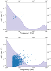 |
Fig. 1 Plots generated using LEGWORK comparing the strain of binaries in two example populations to the LISA sensitivity curve. The first panel is for a population based on Omega Centauri and the second is based on the LMC. Binaries with frequencies below 10−3.6 Hz are not shown. |
Numbers of detectable binaries in globular clusters.
3.2 GW sources in GCs
Table 2 shows the results of 100 000 iterations of four different GCs; each of these samples are individually similar to that in the upper panel of Fig. 1. The physical parameters of these were taken from Baumgardt & Hilker (2018) and Baumgardt & Vasiliev (2021) and compiled in Table C2 of van Zeist et al. (2023), with the metallicity taken to be Z = 0.001. These GCs were chosen as the four most massive GCs in the catalogue located within 10 kpc of Earth.
We expect that each of these GCs will have at least several binaries emitting GWs in the LISA frequency band based on the findings in van Zeist et al. (2023), but Table 2 shows that the amount of binaries that would be detectable by LISA is lower. Specifically, comparing the results in Table 2 to the total numbers of binaries in Table C2 of van Zeist et al. (2023) suggests that only 2–3% of the binaries emitting in the LISA frequency band in these GCs would actually be individually detectable after 10 years of LISA observation.
For Omega Centauri, the most massive GC orbiting the Milky Way (MW), the expected number of detectable binaries is smaller than one even after 10 years of observation. For the other GCs, which are still amongst the most massive in the MW, the probability of a detectable binary being present is 10% or less.
The four GCs we investigated are all between 1010 and 1010.1 years old, so we could compare them to the BPASS data on different types of compact remnants in Table 1 of van Zeist et al. (2023), specifically to the row of the table for a population 1010 years old with metallicity Z = 0.001. Based on those data, we can surmise that any binaries that do appear in our simulations of these GCs have a 93% chance of being a WD–WD, with the next most likely types being BH–WDs followed by NS–WDs. Irrespective of the metallicity, WD–WDs are by far the most common type of compact binaries in BPASS stellar populations of this age.
4 Discussion
4.1 GW sources in the Magellanic Clouds
4.1.1 Comparison to previous research
The LMC results in Sect. 3.1 can be compared to those of Keim et al. (2023), who also evaluate the number of GW sources that would be detectable by LISA in the LMC using the SFH of Harris & Zaritsky (2009), but instead of BPASS use SEBA stellar evolution/population synthesis models (Portegies Zwart & Verbunt 1996; Nelemans et al. 2001b; Toonen et al. 2012).
Keim et al. (2023) predict around 100 to several hundred WD–WD binaries that would be detectable by LISA after 4 yr of observations, depending on assumptions on the stellar distribution. This quantity is at least a factor of 20 higher than our corresponding value in Table 1. Keim et al. (2023) also predict a total of 1–2 × 10⁶ WD–WD binaries emitting with a frequency of at least 10−4 Hz in the LMC (regardless of detectability), where for the same frequency range (which is somewhat wider than our default values for the LISA frequency range) we find around 3–4 × 10⁴ binaries of any type.
Notably, Tang et al. (2024), using BPASS to simulate the WD–WD population of the MW, found a similar discrepancy in the amounts of LISA-detectable WD–WD binaries to what we find here; they found approx. a factor of 20 fewer of these than a comparable study done by Lamberts et al. (2018, 2019) using the stellar evolution and population synthesis code BSE (Hurley et al. 2002).
Another difference between our work and Keim et al. (2023) is that they only looked at WD–WD binaries in their study of LISA GW sources in the LMC, while our data in Table 1 predict at least one detectable NS–WD and BH–WD to be present in the LMC, and non-negligible chances of detectable NS–NS and BH–NS also. This indicates that it is also relevant to study non-WD–WD binaries as potential LISA sources in the LMC.
4.1.2 Mass transfer and common-envelope events in stellar evolution codes
As the discrepancy in the amounts of LISA-detectable WD–WD binaries appears in two separate studies, we believe it is caused by an intrinsic difference in the modelling of stellar evolution between bPass on the one hand and SEBA and BSE on the other. A distinction can be drawn between these two codes in that BPASS models stellar structure in a detailed way throughout the evolution while SEBA and BSE use pre-computed stellar tracks, which do not achieve the same amount of detail in stellar structure but are computationally faster, thus allowing a greater number of different initial parameters to be investigated. However, we note that all stellar evolution models, including detailed ones like BPASS, depend on many assumptions and simplifications about stellar evolution and binary interactions, and in this case it is likely that these assumptions are the most important factor leading to the differing results.
More specifically, we think that the difference in the numbers of detectable WD–WD binaries relates to the treatment of common-envelope events (CEEs) and the stability of mass transfer in the different codes. There have been several recent studies focusing on the implementation of mass transfer in BPASS (Briel et al. 2023; Ghodla & Eldridge 2023), which have found that in BPASS mass transfer is more likely to be stable than in other stellar evolution codes used for population synthesis, and correspondingly fewer CEEs occur. This relates to the different criteria used in stellar evolution codes to determine mass transfer stability: in BPASS a binary is considered to have entered the CEE stage when the radius of the donor (the star that is transferring material to its companion) exceeds the separation between the cores of the two stars (Stevance et al. 2023), while rapid codes such as BSE use analytic calculations based on the evolutionary state of the donor and the binary’s mass ratio to determine stability (Hurley et al. 2002). More details on how BPASS determines mass transfer stability compared to BSE can be found in Sect. 2.3.2 of Tang et al. (2024) and Sect. SI.2.4 of Stevance et al. (2023).
Though Briel et al. (2023) and Ghodla & Eldridge (2023) have focused on binaries that produce BHs and NSs rather than the lighter stars that would produce WDs, it has also been found that in BPASS no CEEs occur at all for binaries with masses below 2 M⊙ (Tang et al. 2024). The prescription used in BPASS for CEEs themselves is also quantitatively different from those used in other codes, as BPASS performs step-by-step calculations of the stellar structure throughout the CEE, and on average tends to lead to less orbital shrinkage than in other codes (Stevance et al. 2023), which also affects the resulting period distribution of compact binaries.
The two differences that we have described between BPASS and other codes – mass transfer being more likely to remain stable rather than forming a CEE, and less angular momentum being lost in CEEs – could in different circumstances either decrease or increase the number of LISA-detectable binaries. Which of these cases applies depends on how efficient the CEE in the simulation is to begin with. In either case, increasing the efficiency of the CEE reduces the amount of angular momentum loss and increases the average separation of the binary after the CEE. Relatively low efficiency means that for many binaries there is so much angular momentum loss that the binary merges before both stars have become compact objects. In this regime, increasing the CEE efficiency increases the amount of LISAdetectable binaries by reducing the amount of early mergers, as found by, for example, Thiele et al. (2023). However, if the CEE efficiency is much higher, then many binaries will remain so wide after the CEE that their GW frequency is too low for LISA to detect, and increasing the CEE efficiency in this regime decreases the amount of LISA-detectable binaries. As we detail in the next subsection, the CEE of BPASS is much more efficient than that of most other population synthesis codes, and so BPASS operates in the second of these regimes while other simulations like those of Thiele et al. (2023) are in the first.
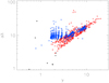 |
Fig. 2 Effective αλ and γ CEE prescription parameters for BPASS models that experience a CEE. The black points are systems that merge in the first binary interaction, the blue points are CEEs from the first binary interaction of a system and the red points are CEEs from the second binary interaction where one of the stars is a WD. |
4.1.3 Details on mass transfer and CEEs in BPASS
To fully understand why BPASS predicts fewer LISA-detectable WD–WDs would require a model-by-model comparison between the BPASS stellar evolution models and those from a rapid population synthesis code. Such a detailed comparison is beyond the scope of this paper; however, we are able to gain some insights by looking at some of the details of the BPASS models.
At solar metallicity, for a simple stellar population with a total mass of 106 M⊙, for the first binary interaction with the primary star as the donor, BPASS predicts there would be 20 907 systems experiencing stable mass transfer, 6783 experiencing a CEE and 223 merging. Then, for the second binary interaction when the donor is the original secondary star, 2361 systems experience stable mass transfer but 7349 experience a CEE.
From these numbers it is clear that in BPASS the first binary interaction is stable (this can also be seen in Fig. 1 of Eldridge et al. 2017). In the BPASS stellar evolution models, mass transfer stability is determined by how the stellar model response to Roche lobe overflow (RLOF). In stable mass transfer the mass loss in RLOF prevents the growth of the stellar radius, which prevents a CEE. However, CEEs can occur through the Darwin instability or if the star continues to grow despite the onset of RLOF. A CEE is assumed to occur when the radius of the stellar model is greater than the binary separation.
In addition to the stability of mass transfer, the second factor affecting our WD–WD period distribution is that the BPASS CEE model is efficient (i.e. it leads to very weak shrinking in the binary orbit during a CEE). To demonstrate this, we include estimated effective values for our CEE models of the αλ and γ values in Fig. 2. We see that the effective αλ values are between 8 and 20 for a CEE in the first binary interaction. Lower values are possible for the second binary interaction, with values from 4 to 30. These values are much higher than those typically used in other stellar evolution codes; for example, the SEBA version of Toonen et al. (2012) assumes αλ = 2 and γ = 1.75, based on calculations by Nelemans et al. (2000) and Nelemans et al. (2001b), respectively. We suspect this is the primary reason why our WD–WD binary population has a dearth of low-period binaries compared to other predictions.
The final two relevant features of the BPASS CEE are that, firstly, the stellar models are computed in a detailed code. With this code it is difficult to just remove the entire envelope in a single timestep as is normally assumed in rapid population synthesis models. Instead, we removed the mass at as high a rate as possible until the envelope collapses and the star is once more smaller than its Roche lobe. The fact this takes time leads to a small spread of possible CEE parameter values, because they are dependent on the stellar and binary parameters. The second feature is that the prescription is closer to the γ-prescription (Nelemans et al. 2000; Nelemans & Tout 2005) in which angular momentum is conserved, rather than the α-prescription (Webbink 1984) which conserves energy; this has also been discussed in Stevance et al. (2023) for its implications on the merger rate of NS binaries.
In summary, the treatment of binary interactions in BPASS is inherently different to most other stellar evolution models. The greater stability of the first binary interaction and the more efficient CEE prescription together lead to fewer short-period WD–WD systems for LISA to detect.
4.1.4 Other studies and discussion on mass transfer assumptions
Temmink et al. (2023) investigated mass transfer stability using the detailed stellar evolution code MESA (Paxton et al. 2011, 2019), and similarly to the BPASS research found that mass transfer in their simulation tended to be more stable than under the assumptions used in other codes such as BSE, but that still a significant fraction of binaries become unstable and likely go through a CEE. Additionally, there has also been recent research using SEBA on the effect of changing assumptions about mass transfer on the resultant population of GW sources (Dorozsmai & Toonen 2024), though like Briel et al. (2023) this research only focused on BH binaries.
Similarly, Wagg et al. (2022c) performed a metastudy (in their Fig. 12) comparing LISA GW detection rate predictions between different stellar evolution codes, showing that these varied by more than an order of magnitude, which is comparable to the differences between codes we have found. Separately, Wagg et al. (2022c) also created their own models that used LEGWORK and the rapid population synthesis code COMPAS (Stevenson et al. 2017; Vigna-Gómez et al. 2018; Riley et al. 2022), and when they varied physics assumptions in these they saw changes of similar magnitude to those we find, though they also only focused on binaries with BHs and NSs.
Some more information on the differences in detectable WD–WD binaries can be found in Fig. 7 of Tang et al. (2024), which compares the WD–WD distribution in chirp mass and period between the BPASS and BSE galaxy models. The BSE distribution shows a trail of binaries with low chirp masses (below 0.3 M⊙) that extends to high frequencies (above 10−4 Hz) that is not present in the BPASS distribution. The diagonal, rather than horizontal, shape of this trail, suggests that these highfrequency binaries are not simply WD–WDs formed at lower frequencies evolving solely through GW emission, but rather that they must have formed at higher frequencies. This in turn suggests they must have undergone some form of a CEE. A similar diagonal trail of low-chirp-mass, high-frequency WD–WDs can also be seen in the SEBA results in Fig. 2 of Nelemans et al. (2001b).
We note that there are several dozen short-period WD–WDs known from EM observations that would have GW frequencies between 10−4 and 10−3 Hz (see e.g. Fig. 1 of Toonen et al. 2012 or the more recent observations catalogued by Burdge et al. 2020). In general, earlier research with SEBA has shown that its results for WD–WD binaries agree quite well with EM observations in terms of the mass and period distribution of these systems, though these EM observations are subject to observational biases (Nelemans et al. 2001b; Toonen et al. 2012).
Aside from differences in CEEs and mass transfer, BPASS also does not include magnetic wind braking (Rappaport et al. 1983), an effect that can cause binaries to lose angular momentum. By contrast, SEBA (Portegies Zwart & Verbunt 1996) and BSE (Hurley et al. 2002) do include this effect in their models. However, we do not expect this effect to be as important as the common-envelope prescription for the WD–WD binaries observable by LISA.
4.1.5 Effects of a stronger common-envelope prescription
To investigate the effects that differences in CEE prescriptions could have on the amounts of binaries detectable by LISA, we made several kinds of simple modifications to our BPASS populations to simulate a stronger CEE prescription (i.e. one that produces more orbital shrinkage) than that of bPass. Table 3 shows the results of 1000 random samplings of the LMC, including both the fiducial model (identical to that shown in Table 1) and three adjusted models.
In each of the three adjusted models, the orbital frequency of some of the binaries in the population is increased, simulating a situation in which a CEE led to stronger orbital shrinkage for those binaries. In Model A, we randomly selected 10% of the binaries in the BPASS output population and increased their frequency by a factor of 10. In Model B, we did the same except we randomly selected 20% of the binaries instead. In Model C, we increased the frequency of all of the binaries by a factor of 3.
In Table 3, we can see that in the alternate models, even those where we only adjusted 10% of the binaries in the population, the number of binaries detectable by LISA is dramatically increased. For Model A, there are around 45 times as many detectable binaries in total compared to the fiducial model, and for Models B and C the factors of increase are around 90 and 20, respectively. The factors are similar after both 4 and 10 years of observation.
For Model C (with a threefold frequency increase) the factor by which the amount of detectable binaries is increased is fairly consistent across each of the binary types, but for Models A and B (with a tenfold frequency increase) the lighter binary types are increased more than the heavier binary types, which gives an indication of differences in the underlying period distributions of the different binary types, particularly at frequencies around 10−4 and 10−3 Hz where binaries may not be detectable in the fiducial model but would be with a tenfold frequency increase. BH–BHs are increased by a factor of around 10 in Model A and 20 in Model B, while WD–WDs are increased by a factor of around 50 in Model A and 110 in Model B.
The key result of this test is that amounts of detectable WD–WD binaries predicted by the alternate models, particularly Models A and B, fall within the range of the SEBA results of Keim et al. (2023), who predicted from one hundred to several hundred detectable WD–WDs (depending on assumptions in their models) after four years of LISA observation. This gives us further confidence that the main factor leading to the difference between our fiducial results and those of Keim et al. (2023) is the treatment of mass transfer and CEEs in BPASS versus SEBA, as with these simple approximations of stronger CEEs we can make the BPASS results match those from SEBA.
However, we note that these implementations of stronger CEEs are highly simplified and that there are a number of caveats. For example, for Models A and B we selected the binaries that we applied the frequency increase to randomly from across all binary types, while in reality the effects of a CEE would depend on the properties of the binary and be different for different binary types. Additionally, the three alternate models do not take into account that the increase in frequency from stronger CEEs would cause the binaries to merge more quickly through emission of GWs, which would affect the age distribution of these binaries.
Numbers of detectable binaries for LMC models with more orbital shrinkage.
Numbers of detectable binaries in the SMC and LMC with confusion noise set to zero.
4.1.6 Effects of confusion noise models
In our detectability calculations, we used the LISA sensitivity curve constructed by Robson et al. (2019). This curve gives the strain sensitivity of LISA at different frequencies and consists of two components: the instrumental noise (noise originating from physical properties of the detector itself) and foreground confusion noise, which consists of the overlapping signals of many Galactic binaries (mostly WD–WDs) that are individually too weak to resolve. This noise therefore depends on the population of binary sources present in the Galaxy.
The sensitivity curve of Robson et al. (2019) includes a formulation of the confusion noise from Cornish & Robson (2017), who calculated the confusion noise using a galaxy model constructed using SEBA. As established in the preceding sections of this paper, stellar populations modelled using BPASS yield fewer binaries in the LISA frequency range compared to SEBA. Therefore, it is not entirely accurate for us to be calculating the detectability of BPASS stellar populations against a sensitivity curve that was calculated using a SEBA galaxy model. This is because we would expect the confusion noise to be smaller in magnitude if it was calculated using a BPASS galaxy model like that of Tang et al. (2024), as the binaries contributing to the unresolved Galactic foreground would be fewer in number.
With less confusion noise, the number of binaries that would be detectable by LISA would increase. Constructing a new LISA sensitivity curve using BPASS is beyond the scope of this paper, but we can calculate the detectability in a maximally optimistic case by simply assuming the confusion noise to be zero. The results of this are shown in Table 4, where we repeated our calculations of the number of detectable binaries in the LMC and SMC (as in Table 1) but with the confusion noise set to zero in LEGWORK. The values that would be found using BPASs-based confusion noise must then be between those using SEBA-based confusion noise in Table 1 as a lower bound and those using zero confusion noise in Table 4 as an upper bound.
As expected, the numbers of detectable binaries in Table 4 are higher than those in the fiducial case for both the SMC and the LMC and for both 4 and 10 years of observation. However, the total number of binaries only increases by approximately 30% on average, and in none of the cases does the increase exceed 50%. Looking at WD–WDs alone, the increase is even smaller. Therefore, even in this most optimistic case, altering the confusion noise does not come close to resolving the differences between our results and those of Keim et al. (2023). Hence, we conclude that recalculating the Robson et al. (2019) noise curve to use a BPASS-based confusion noise would not affect our previous conclusions.
4.2 GW sources in globular clusters
4.2.1 Comparison to previous research
We can compare our GC results in Sect. 3.2 to the results of Kremer et al. (2018), who used Cluster Monte Carlo (CMC; Joshi et al. 2000; Rodriguez et al. 2022) simulations for the gravitational evolution of a GC along with the stellar evolution codes BSE and its single-star evolution counterpart SSE (Hurley et al. 2000) to predict that around 14–21 binaries across all MW GCs would be detectable by LISA after 4 years, including 4 to 6 WD–WDs. An earlier study by Willems et al. (2007), who used GC simulations by Ivanova et al. (2006) using CMC and the stellar evolution code STARTRACK (Belczynski et al. 2002, 2008), found even higher numbers, specifically finding several dozen observable WD–WDs across all MW GCs, even with the constraint of only looking at eccentric binaries.
We did not perform an equivalent computation for all MW GCs, particularly because for less massive GCs the uncertainty from the limited number of iterations would dominate the actual rates. However, based on our results in Table 2 using some of the most massive GCs, we can say that our total number of expected binaries for all ~150 known MW GCs, particularly for only 4 years of observation, would likely be of the order of one or fewer. Therefore, as with the Magellanic Clouds, we see a lower number of detectable binaries in our simulations compared to previous simulations using different methods.
The size of this discrepancy, a factor of 20 to 40, is also comparable to what we find for the Magellanic Clouds. This means that, if we account for the differences in stellar evolution between BPASS and other stellar evolution codes like BSE, which we discussed in Sect. 4.1, our numbers would become similar to those of Kremer et al. (2018) and Willems et al. (2007).
4.2.2 Dynamical interactions
As for the Magellanic Clouds, the intrinsic differences between BPASS and other population synthesis codes in terms of stellar evolution are a probable explanation for our expected numbers of detectable binaries in GCs being lower than those found by other groups. Because the difference between our results and those from other stellar evolution codes is similar in magnitude for both GCs and the Magellanic Clouds, it is possible that the stellar evolution is also the largest contributing factor for GCs. However, for our simulations of GCs there is an additional factor that does not apply to the Magellanic Clouds and could also affect the binary population and the number of detectable GW sources: dynamical interactions.
To be more specific, the BPASS models that we used consist of isolated binaries, wherein the stellar evolution is only affected by processes inside the binary, without any effects from external forces. For stellar environments with a relatively low density, such as the MW disk of Tang et al. (2024) or the Magellanic Clouds discussed in Sect. 4.1 of this paper, the assumption of isolated binary evolution is reasonable. However, in GCs the stellar density is sufficiently high that the chance of a binary interacting with another stellar system during its evolution is non-negligible.
These dynamical interactions have been studied through simulations of the gravitational evolution of a GC, for which several different methods have been used in the literature. The most accurate method is to fully model the gravitational effect that each star or compact remnant in the cluster has on every other one using an N-body simulation. A number of different codes that perform this exist, including the NBODY family of codes, which have a long history of development starting from NBODY1 (Aarseth 1963), with the most recent version being NBODY7 (Aarseth 2012).
However, N-body simulations have a significant limitation in the high amount of computational time they require. This prompted the development of another type of GC dynamical simulation, which approximates the N-body simulations numerically with a significantly shorter computational time, particularly the Monte Carlo method originally developed by Hénon (1971a,b). There are currently two commonly used computational implementations of this method, which are the aforementioned CMC (Joshi et al. 2000; Rodriguez et al. 2022) and MOCCA (Giersz 1998; Hypki & Giersz 2013).
4.2.3 Effects of dynamical interactions on binaries
Dynamical interactions can have various effects on the binary population and consequently the GW signal of the GC. It is expected the cumulative effects of many minor interactions will result in a general hardening of the binary population; that is, an increase in the average frequency (Heggie 1975; Ivanova et al. 2006, 2008; Portegies Zwart et al. 2010). Such an effect would tend to shift more binaries into the LISA frequency range, increasing the number of those that would be detectable, and therefore this could be a contributing factor to the differences between our results and those of Kremer et al. (2018).
However, dynamical interactions could also result in both the formation of new binaries through tidal capture and the unbinding of existing ones. The relative importance of these processes varies depending on the types of binaries considered. Binaries with BHs and NSs that occur in GCs are predicted to mostly be dynamically formed (e.g. Kundu et al. 2002; Pooley et al. 2003; Sadowski et al. 2008; Ivanova et al. 2008; Morscher et al. 2015). This is corroborated when we compare the BPASS results to those from CMC simulations: in Table 1 of Kremer et al. (2018) the predictions for detectable BH–BH and NS–NS binaries range from being the same those for WD–WDs to a factor of 10 lower, but in Table 1 of van Zeist et al. (2023) the differences are larger: the NS–NS rates are two to four orders of magnitude lower than those of WD–WDs, and BH–BHs around five orders of magnitude lower than WD–WDs.
The effect of dynamical interactions on WD–WD evolution and rates is less clear from the literature. This is partly because of differing results from different studies and partly because many of the studies on this topic do not directly look at WD–WD binaries, but rather at cataclysmic variables (CVs), particularly those of the AM Canum Venaticorum (AM CVn) type; these are mass-transferring binaries with a WD and a living star, which are easier to detect in EM than WD–WDs. While CVs are not generally thought to evolve directly to GW-emitting WD–WD binaries, they originate from similar types of stellar systems, and therefore the population of EM-observable CVs in a cluster can be indicative of its population of GW-observable WD–WDs.
For example, based on X-ray observations of CVs in GCs, different analyses by Pooley & Hut (2006) and Cheng et al. (2018) reached different conclusions, with the former suggesting that most CVs in GCs were of dynamical origin and the latter the opposite (i.e. that most were of primordial origin); both analyses have potential caveats due to observational limits and biases (Heinke et al. 2020; Belloni & Rivera Sandoval 2021). A recent study by Bao et al. (2023), using X-ray observations to study the period distribution of CVs in the GC 47 Tucanae, did find evidence that a significant fraction of these CVs were likely dynamically formed.
In terms of theoretical predictions based on simulations, Knigge (2012) argues based on a review of a number of different simulations that most CVs in GCs are likely dynamically formed. Similarly, studies using CMC (Ivanova et al. 2006) and MOCCA (Belloni et al. 2016) did find that respectively 60% and 100% of the surviving CV models in their simulations had undergone some sort of dynamical interaction. However, this does not necessarily mean that dynamical interactions increase the number of CVs in a cluster, as Belloni et al. (2019) and Kremer et al. (2020), using the MOCCA and CMC types of Monte Carlo simulations, respectively, found that dynamical destruction of CVs in GCs was stronger than dynamical creation. Kremer et al. (2020) also found that the amount of WD–WD binaries in a GC decreases with increasing dynamical interactions. Finally, we note that Shara & Hurley (2006), using N-body simulations, found 5–6 times more short-period WD–WDs in a GC population compared to the field but 2–3 times fewer CVs, which highlights that trends in EM-observable CVs do not necessarily correlate with those in GW-observable WD–WDs.
As an example, to go into more numerical detail, Kremer et al. (2020) predict 100 to 200 WD–WDs per 106 M⊙ in typical GCs, depending on the cluster’s density, using cosmic (Breivik et al. 2020a), a rapid population synthesis code derived from BSE, and using CMC to model the effects of dynamical interactions. By comparison, Thiele et al. (2023), also using COSMIC but looking at MW disk populations without dynamical interactions, predict of the order of 500 to 10 000 WD–WDs per 106 M⊙, depending on metallicity and binary evolution assumptions. Meanwhile, Shara & Hurley (2006), using BSE and N-body dynamics, predict 500 WD–WDs per 106 M⊙ for a field population but 3000 WD–WDs per 106 M⊙ for a GC.
In general, both EM observations and simulation-based predictions in the literature seem inconclusive about the effects of dynamical interactions on WD–WD binaries, including whether this would result in more or fewer WD–WDs occurring in GCs than in the field. Our own results broadly align with this in the sense that the discrepancy between our WD–WD predictions in this section and the CMC-BSE predictions of Kremer et al. (2018) is of a similar magnitude (a factor of 20–40) to the discrepancy between our results for the Magellanic Clouds and the SEBA and BSE studies discussed in Sect. 4.1 – despite dynamical interactions being a factor for GCs but negligible for the Magellanic Clouds.
The consistency of the disparity across both the GC and Magellanic simulations suggests that the effect of dynamical interactions on the total number of WD–WD binaries that would be detectable by LISA is likely smaller in magnitude than the effect of the differences in the treatment of stellar evolution between bPass and SEBA or BSE. The reason for this is that, if the effect of dynamical interactions was in fact significant, we would expect the discrepancy between our results and previous research to be larger for the GCs than for the Magellanic Clouds. However, this is a very simple estimation and fully understanding the impact of the inclusion of dynamical interactions on the binary population synthesis results merits further research.
4.2.4 Ejections and cluster mass loss
Aside from their effect on the evolution of individual binaries, the lack of dynamical interactions in our simulations could also be affecting our results through their effect on the overall mass of the cluster. Specifically, as described in Sect. 2.2, we computed the initial mass of a cluster from the current mass using BPASS data files that account for the mass lost by individual stellar systems through their evolution. However, there is an additional way in which GCs can lose mass, in that dynamical interactions can cause stars or compact remnants, particularly heavier objects like BHs, to be ejected from the cluster (Portegies Zwart & McMillan 2000). A broad overview of the mechanisms whereby objects can be ejected from GCs is given in Sect. 2 of Weatherford et al. (2023).
Taking this effect into account would increase the mass lost by a GC over time, and thus for a given current mass would increase the computed initial mass, which would increase the present-day amount of binaries in our simulations. This could therefore account for some of the difference between our predicted numbers of binaries and those of the CMC simulations of Kremer et al. (2018).
However, the magnitude of the mass loss due to dynamical ejections varies significantly between different simulations in the literature as it depends on numerous properties of the cluster involved, such as its mass, radius and Galactic location. One particular relevant parameter is the dynamical relaxation timescale, which is proportional to the cluster mass if its density is held constant. For example, Shara & Hurley (2006), from an N-body simulation of a single GC, found about 75% of objects were ejected after 15 Gyr and 90% after 20 Gyr, and the total mass of the cluster was only about 20% of its initial mass after 16 Gyr. However, Weatherford et al. (2023) performed CMC simulations of GCs, where the clusters most analogous to those of Shara & Hurley (2006) – with similar densities and Galactocentric distances, but with eight times as many objects, leading to a slower dynamical timescale – had only 10–20% of objects ejected after 14 Gyr, with the cluster masses being about 50% of their initial masses at that time.
We also note that Pijloo et al. (2015) created a code to calculate the initial mass of a cluster based on its current parameters using a combination of Monte Carlo simulations and semianalytical methods; this code uses a simple approximation of mass loss from stellar evolution which is outlined in Alexander et al. (2014), but it could potentially be adapted to use the more detailed BPASS mass loss calculations in the future.
5 Conclusions
In summary, we draw the following conclusions:
The Magellanic Clouds and GCs are potential hosts of GW sources that would be detectable by LISA. The BPASS simulations suggest the Magellanic sources would be a mixture of NS–WDs, WD–WDs and potentially other types of binaries such as BH–WDs, while the GC sources would be predominantly WD–WDs. This indicates that non-WD–WD binaries should not be ignored in GW analyses of the Magellanic Clouds;
We find a few dozen times fewer detectable WD–WD binaries in the LMC than a comparable study by Keim et al. (2023), who used the stellar evolution/population synthesis code SEBA. A similar discrepancy was found by Tang et al. (2024) when they compared their BPASS model for the WD–WD binaries in the MW disk to the results of Lamberts et al. (2018, 2019), who used BSE, which indicates that the discrepancy originates from the stellar evolution codes;
More specifically, we believe that the discrepancy between our results and the earlier research that used SEBA and BSE originates from differences in the treatment of stellar evolution, particularly relating to CEEs and the stability of mass transfer. Tests we conducted that involved simulating a stronger CEE in BPASS give us further confidence in this explanation;
For GCs, based solely on the isolated binary evolution of BPASS, we predict that there will be fewer than one detectable binary even for the most massive GC, Omega Centauri. These numbers are a few dozen times lower than those predicted by Kremer et al. (2018), who used CMC to simulate GC dynamics and SSE and BSE for stellar evolution. The discrepancy is larger for binary types other than WD–WDs, which are more likely to be affected by GC dynamical interactions;
Different studies in the literature that used different methods with various cluster mass and density assumptions find that GC dynamical interactions can increase and sometimes decrease the number of detectable WD–WDs by a factor of a few. Based on the consistency in the size of the discrepancy between BPASS and other codes regarding the number of detectable WD–WDs in both the Magellanic Cloud and GC simulations in our study, we also do not see a clear effect from the inclusion or exclusion of GC dynamics on the detectability of WD–WDs. However, we do see that the stellar evolution differences affect the WD–WD detection rates in GCs by a factor of 20–40.
Data availability
The BPASS dataset can be downloaded from https://bpass.auckland.ac.nz. The LEGWORK code can be found at https://github.com/TeamLEGWORK/LEGWORK. Other data underlying this article will be shared upon reasonable request to the corresponding author.
Acknowledgements
WGJvZ acknowledges support from Radboud University, the European Research Council (ERC) under the European Union’s Horizon 2020 research and innovation programme (grant agreement No. 725246), Dutch Research Council grant 639.043.514 and the University of Auckland. JJE acknowledges support from Marsden Fund Council grant MFP-UOA2131 managed through the Royal Society of New Zealand Te Apārangi.
References
- Aarseth, S. J. 1963, MNRAS, 126, 223 [NASA ADS] [Google Scholar]
- Aarseth, S. J. 2012, MNRAS, 422, 841 [NASA ADS] [CrossRef] [Google Scholar]
- Abbott, R., Abbott, T. D., Acernese, F., et al. 2023, Phys. Rev. X, 13, 041039 [Google Scholar]
- Alexander, P. E. R., Gieles, M., Lamers, H. J. G. L. M., & Baumgardt, H. 2014, MNRAS, 442, 1265 [NASA ADS] [CrossRef] [Google Scholar]
- Amaro-Seoane, P., Audley, H., Babak, S., et al. 2017, arXiv e-prints [arXiv:1702.00786] [Google Scholar]
- Amaro-Seoane, P., Andrews, J., Arca Sedda, M., et al. 2023, Liv. Rev. Relativ., 26, 2 [NASA ADS] [CrossRef] [Google Scholar]
- Auclair, P., Bacon, D., Baker, T., et al. 2023, Liv. Rev. Relativ., 26, 5 [NASA ADS] [CrossRef] [Google Scholar]
- Bao, T., Li, Z., & Cheng, Z. 2023, MNRAS, 521, 4257 [NASA ADS] [CrossRef] [Google Scholar]
- Bastian, N., & Lardo, C. 2018, ARA&A, 56, 83 [Google Scholar]
- Baumgardt, H., & Hilker, M. 2018, MNRAS, 478, 1520 [Google Scholar]
- Baumgardt, H., & Vasiliev, E. 2021, MNRAS, 505, 5957 [NASA ADS] [CrossRef] [Google Scholar]
- Belczynski, K., Kalogera, V., & Bulik, T. 2002, ApJ, 572, 407 [NASA ADS] [CrossRef] [Google Scholar]
- Belczynski, K., Kalogera, V., Rasio, F. A., et al. 2008, ApJS, 174, 223 [Google Scholar]
- Belczynski, K., Benacquista, M., & Bulik, T. 2010, ApJ, 725, 816 [NASA ADS] [CrossRef] [Google Scholar]
- Belloni, D., Giersz, M., Askar, A., Leigh, N., & Hypki, A. 2016, MNRAS, 462, 2950 [NASA ADS] [CrossRef] [Google Scholar]
- Belloni, D., Giersz, M., Rivera Sandoval, L. E., Askar, A., & Ciecieląg, P. 2019, MNRAS, 483, 315 [NASA ADS] [CrossRef] [Google Scholar]
- Belloni, D. & Rivera Sandoval, L. 2021, in The Golden Age of Cataclysmic Variables and Related Objects V, 2, 13 [Google Scholar]
- Benacquista, M. J., & Downing, J. M. B. 2013, Liv. Rev. Relativ., 16, 4 [NASA ADS] [CrossRef] [Google Scholar]
- Benacquista, M. J., Portegies Zwart, S., & Rasio, F. A. 2001, Class. Quant. Grav., 18, 4025 [NASA ADS] [CrossRef] [Google Scholar]
- Breivik, K., Coughlin, S., Zevin, M., et al. 2020a, ApJ, 898, 71 [Google Scholar]
- Breivik, K., Mingarelli, C. M. F., & Larson, S. L. 2020b, ApJ, 901, 4 [NASA ADS] [CrossRef] [Google Scholar]
- Briel, M. M., Stevance, H. F., & Eldridge, J. J. 2023, MNRAS, 520, 5724 [Google Scholar]
- Burdge, K. B., Prince, T. A., Fuller, J., et al. 2020, ApJ, 905, 32 [Google Scholar]
- Cheng, Z., Li, Z., Xu, X., & Li, X. 2018, ApJ, 858, 33 [NASA ADS] [CrossRef] [Google Scholar]
- Colpi, M., Danzmann, K., Hewitson, M., et al. 2024, arXiv e-prints [arXiv:2402.07571] [Google Scholar]
- Cornish, N., & Robson, T. 2017, in Journal of Physics Conference Series, 840, 012024 [NASA ADS] [CrossRef] [Google Scholar]
- Dorozsmai, A., & Toonen, S. 2024, MNRAS, 530, 3706 [NASA ADS] [CrossRef] [Google Scholar]
- Eldridge, J. J. 2012, MNRAS, 422, 794 [NASA ADS] [CrossRef] [Google Scholar]
- Eldridge, J. J., Stanway, E. R., Xiao, L., et al. 2017, PASA, 34, e058 [Google Scholar]
- Ghodla, S., & Eldridge, J. J. 2023, MNRAS, 523, 1711 [NASA ADS] [CrossRef] [Google Scholar]
- Ghodla, S., van Zeist, W. G. J., Eldridge, J. J., Stevance, H. F., & Stanway, E. R. 2022, MNRAS, 511, 1201 [NASA ADS] [CrossRef] [Google Scholar]
- Giersz, M. 1998, MNRAS, 298, 1239 [NASA ADS] [CrossRef] [Google Scholar]
- Harris, J., & Zaritsky, D. 2004, AJ, 127, 1531 [NASA ADS] [CrossRef] [Google Scholar]
- Harris, J., & Zaritsky, D. 2009, AJ, 138, 1243 [NASA ADS] [CrossRef] [Google Scholar]
- Heggie, D. C. 1975, MNRAS, 173, 729 [NASA ADS] [CrossRef] [Google Scholar]
- Heggie, D., & Hut, P. 2003, The Gravitational Million-Body Problem: A Multidisciplinary Approach to Star Cluster Dynamics [Google Scholar]
- Heinke, C. O., Ivanov, M. G., Koch, E. W., et al. 2020, MNRAS, 492, 5684 [NASA ADS] [CrossRef] [Google Scholar]
- Hénon, M. 1971a, Ap&SS, 13, 284 [Google Scholar]
- Hénon, M. H. 1971b, Ap&SS, 14, 151 [Google Scholar]
- Hils, D., Bender, P. L., & Webbink, R. F. 1990, ApJ, 360, 75 [CrossRef] [Google Scholar]
- Hurley, J. R., Pols, O. R., & Tout, C. A. 2000, MNRAS, 315, 543 [Google Scholar]
- Hurley, J. R., Tout, C. A., & Pols, O. R. 2002, MNRAS, 329, 897 [Google Scholar]
- Hypki, A., & Giersz, M. 2013, MNRAS, 429, 1221 [NASA ADS] [CrossRef] [Google Scholar]
- Ivanova, N., Heinke, C. O., Rasio, F. A., et al. 2006, MNRAS, 372, 1043 [CrossRef] [Google Scholar]
- Ivanova, N., Heinke, C. O., Rasio, F. A., Belczynski, K., & Fregeau, J. M. 2008, MNRAS, 386, 553 [NASA ADS] [CrossRef] [Google Scholar]
- Joshi, K. J., Rasio, F. A., & Portegies Zwart, S. 2000, ApJ, 540, 969 [NASA ADS] [CrossRef] [Google Scholar]
- Keim, M. A., Korol, V., & Rossi, E. M. 2023, MNRAS, 521, 1088 [NASA ADS] [CrossRef] [Google Scholar]
- Knigge, C. 2012, Mem. Soc. Astron. Italiana, 83, 549 [NASA ADS] [Google Scholar]
- Korol, V., Rossi, E. M., Groot, P. J., et al. 2017, MNRAS, 470, 1894 [NASA ADS] [CrossRef] [Google Scholar]
- Korol, V., Toonen, S., Klein, A., et al. 2020, A&A, 638, A153 [NASA ADS] [CrossRef] [EDP Sciences] [Google Scholar]
- Kremer, K., Chatterjee, S., Breivik, K., et al. 2018, Phys. Rev. Lett., 120, 191103 [NASA ADS] [CrossRef] [Google Scholar]
- Kremer, K., Ye, C. S., Rui, N. Z., et al. 2020, ApJS, 247, 48 [NASA ADS] [CrossRef] [Google Scholar]
- Kroupa, P., Tout, C. A., & Gilmore, G. 1993, MNRAS, 262, 545 [NASA ADS] [CrossRef] [Google Scholar]
- Kundu, A., Maccarone, T. J., & Zepf, S. E. 2002, ApJ, 574, L5 [NASA ADS] [CrossRef] [Google Scholar]
- Kupfer, T., Korol, V., Littenberg, T. B., et al. 2024, ApJ, 963, 100 [NASA ADS] [CrossRef] [Google Scholar]
- Lamberts, A., Garrison-Kimmel, S., Hopkins, P. F., et al. 2018, MNRAS, 480, 2704 [NASA ADS] [CrossRef] [Google Scholar]
- Lamberts, A., Blunt, S., Littenberg, T. B., et al. 2019, MNRAS, 490, 5888 [NASA ADS] [CrossRef] [Google Scholar]
- Lau, M. Y. M., Mandel, I., Vigna-Gómez, A., et al. 2020, MNRAS, 492, 3061 [NASA ADS] [CrossRef] [Google Scholar]
- Lipunov, V. M., Postnov, K. A., & Prokhorov, M. E. 1987, A&A, 176, L1 [NASA ADS] [Google Scholar]
- Littenberg, T. B., Cornish, N. J., Lackeos, K., & Robson, T. 2020, Phys. Rev. D, 101, 123021 [NASA ADS] [CrossRef] [Google Scholar]
- Milone, A. P., & Marino, A. F. 2022, Universe, 8, 359 [NASA ADS] [CrossRef] [Google Scholar]
- Moe, M., & Di Stefano, R. 2017, ApJS, 230, 15 [Google Scholar]
- Morscher, M., Pattabiraman, B., Rodriguez, C., Rasio, F. A., & Umbreit, S. 2015, ApJ, 800, 9 [NASA ADS] [CrossRef] [Google Scholar]
- Nelemans, G., & Tout, C. A. 2005, MNRAS, 356, 753 [NASA ADS] [CrossRef] [Google Scholar]
- Nelemans, G., Verbunt, F., Yungelson, L. R., & Portegies Zwart, S. F. 2000, A&A, 360, 1011 [NASA ADS] [Google Scholar]
- Nelemans, G., Yungelson, L. R., & Portegies Zwart, S. F. 2001a, A&A, 375, 890 [NASA ADS] [CrossRef] [EDP Sciences] [Google Scholar]
- Nelemans, G., Yungelson, L. R., Portegies Zwart, S. F., & Verbunt, F. 2001b, A&A, 365, 491 [NASA ADS] [CrossRef] [EDP Sciences] [Google Scholar]
- Nissanke, S., Vallisneri, M., Nelemans, G., & Prince, T. A. 2012, ApJ, 758, 131 [NASA ADS] [CrossRef] [Google Scholar]
- Paczyński, B. 1967, Acta Astron., 17, 287 [NASA ADS] [Google Scholar]
- Paxton, B., Bildsten, L., Dotter, A., et al. 2011, ApJS, 192, 3 [Google Scholar]
- Paxton, B., Smolec, R., Schwab, J., et al. 2019, ApJS, 243, 10 [Google Scholar]
- Pijloo, J. T., Portegies Zwart, S. F., Alexander, P. E. R., et al. 2015, MNRAS, 453, 605 [NASA ADS] [CrossRef] [Google Scholar]
- Pooley, D., & Hut, P. 2006, ApJ, 646, L143 [NASA ADS] [CrossRef] [Google Scholar]
- Pooley, D., Lewin, W. H. G., Anderson, S. F., et al. 2003, ApJ, 591, L131 [NASA ADS] [CrossRef] [Google Scholar]
- Portegies Zwart, S. F., & McMillan, S. L. W. 2000, ApJ, 528, L17 [Google Scholar]
- Portegies Zwart, S. F., & Verbunt, F. 1996, A&A, 309, 179 [NASA ADS] [Google Scholar]
- Portegies Zwart, S. F., McMillan, S. L. W., & Gieles, M. 2010, ARA&A, 48, 431 [NASA ADS] [CrossRef] [Google Scholar]
- Rappaport, S., Verbunt, F., & Joss, P. C. 1983, ApJ, 275, 713 [Google Scholar]
- Riley, J., Agrawal, P., Barrett, J. W., et al. 2022, ApJS, 258, 34 [NASA ADS] [CrossRef] [Google Scholar]
- Robson, T., Cornish, N. J., & Liu, C. 2019, Class. Quant. Grav., 36, 105011 [NASA ADS] [CrossRef] [Google Scholar]
- Rodriguez, C. L., Weatherford, N. C., Coughlin, S. C., et al. 2022, ApJS, 258, 22 [NASA ADS] [CrossRef] [Google Scholar]
- Roebber, E., Buscicchio, R., Vecchio, A., et al. 2020, ApJ, 894, L15 [NASA ADS] [CrossRef] [Google Scholar]
- Ruiter, A. J., Belczynski, K., Benacquista, M., Larson, S. L., & Williams, G. 2010, ApJ, 717, 1006 [NASA ADS] [CrossRef] [Google Scholar]
- Sadowski, A., Belczynski, K., Bulik, T., et al. 2008, ApJ, 676, 1162 [NASA ADS] [CrossRef] [Google Scholar]
- Schneider, R., Ferrari, V., Matarrese, S., & Portegies Zwart, S. F. 2001, MNRAS, 324, 797 [NASA ADS] [CrossRef] [Google Scholar]
- Shara, M. M., & Hurley, J. R. 2006, ApJ, 646, 464 [NASA ADS] [CrossRef] [Google Scholar]
- Stanway, E. R., & Eldridge, J. J. 2018, MNRAS, 479, 75 [NASA ADS] [CrossRef] [Google Scholar]
- Stanway, E. R., & Eldridge, J. J. 2023, MNRAS, 522, 4430 [NASA ADS] [CrossRef] [Google Scholar]
- Stevance, H. F., Eldridge, J. J., Stanway, E. R., et al. 2023, Nat. Astron., 7, 444 [NASA ADS] [CrossRef] [Google Scholar]
- Stevenson, S., Vigna-Gómez, A., Mandel, I., et al. 2017, Nat. Commun., 8, 14906 [Google Scholar]
- Tang, P., Eldridge, J. J., Meyer, R., et al. 2024, MNRAS, 534, 1707 [NASA ADS] [CrossRef] [Google Scholar]
- Temmink, K. D., Pols, O. R., Justham, S., Istrate, A. G., & Toonen, S. 2023, A&A, 669, A45 [NASA ADS] [CrossRef] [EDP Sciences] [Google Scholar]
- Thiele, S., Breivik, K., Sanderson, R. E., & Luger, R. 2023, ApJ, 945, 162 [NASA ADS] [CrossRef] [Google Scholar]
- Toonen, S., Nelemans, G., & Portegies Zwart, S. 2012, A&A, 546, A70 [NASA ADS] [CrossRef] [EDP Sciences] [Google Scholar]
- van Zeist, W. G. J., Eldridge, J. J., & Tang, P. N. 2023, MNRAS, 524, 2836 [NASA ADS] [CrossRef] [Google Scholar]
- Vigna-Gómez, A., Neijssel, C. J., Stevenson, S., et al. 2018, MNRAS, 481, 4009 [Google Scholar]
- Wagg, T., Breivik, K., & de Mink, S. 2022a, J. Open Source Softw., 7, 3998 [NASA ADS] [CrossRef] [Google Scholar]
- Wagg, T., Breivik, K., & de Mink, S. E. 2022b, ApJS, 260, 52 [NASA ADS] [CrossRef] [Google Scholar]
- Wagg, T., Broekgaarden, F. S., de Mink, S. E., et al. 2022c, ApJ, 937, 118 [NASA ADS] [CrossRef] [Google Scholar]
- Weatherford, N. C., Kıroğlu, F., Fragione, G., et al. 2023, ApJ, 946, 104 [NASA ADS] [CrossRef] [Google Scholar]
- Webbink, R. F. 1984, ApJ, 277, 355 [NASA ADS] [CrossRef] [Google Scholar]
- Willems, B., Kalogera, V., Vecchio, A., et al. 2007, ApJ, 665, L59 [NASA ADS] [CrossRef] [Google Scholar]
All Tables
Numbers of detectable binaries in the SMC and LMC with confusion noise set to zero.
All Figures
|
Fig. 1 Plots generated using LEGWORK comparing the strain of binaries in two example populations to the LISA sensitivity curve. The first panel is for a population based on Omega Centauri and the second is based on the LMC. Binaries with frequencies below 10−3.6 Hz are not shown. |
| In the text | |
|
Fig. 2 Effective αλ and γ CEE prescription parameters for BPASS models that experience a CEE. The black points are systems that merge in the first binary interaction, the blue points are CEEs from the first binary interaction of a system and the red points are CEEs from the second binary interaction where one of the stars is a WD. |
| In the text | |
Current usage metrics show cumulative count of Article Views (full-text article views including HTML views, PDF and ePub downloads, according to the available data) and Abstracts Views on Vision4Press platform.
Data correspond to usage on the plateform after 2015. The current usage metrics is available 48-96 hours after online publication and is updated daily on week days.
Initial download of the metrics may take a while.