| Issue |
A&A
Volume 691, November 2024
|
|
|---|---|---|
| Article Number | A261 | |
| Number of page(s) | 9 | |
| Section | Extragalactic astronomy | |
| DOI | https://doi.org/10.1051/0004-6361/202451510 | |
| Published online | 19 November 2024 | |
Uncertainty of the white dwarf astrophysical gravitational wave background
1
Department of Astrophysics/IMAPP, Radboud University, PO Box 9010 6500 GL Nijmegen, The Netherlands
2
Institute of Astronomy, KU Leuven, Celestijnenlaan 200D, 3001 Leuven, Belgium
3
SRON, Netherlands Institute for Space Research, Niels Bohrweg 4, 2333 CA Leiden, The Netherlands
⋆ Corresponding author; This email address is being protected from spambots. You need JavaScript enabled to view it.
Received:
15
July
2024
Accepted:
28
September
2024
Abstract
Context. The astrophysical gravitational wave background (AGWB) is a stochastic gravitational wave (GW) signal emitted by different populations of in-spiralling binary systems containing compact objects throughout the Universe. In the frequency range between 10−4 and 10−1 hertz (Hz), it will be detected by future space-based gravitational wave detectors, such as Laser Interferometer Space Antenna (LISA). In a recent work, we concluded that the white dwarf (WD) contribution to the AGWB dominates that of black holes (BHs) and neutron stars (NSs).
Aims. We aim to investigate the uncertainties of the WD AGWB that arise from the use of different stellar metallicities, star formation rate density (SFRD) models, and binary evolution models.
Methods. We used the code we previously developed to determine the WD component of the AGWB. We used a metallicity-dependent SFRD based on an earlier work to construct five different SFRD models. We used four different population models based on a range of common-envelope treatments and six different metallicities for each model.
Results. For all possible combinations, the WD component of the AGWB is dominant over other populations of compact objects. The effects of metallicity and population model are less significant than the effect of a (metallicity dependent) SFRD model. We find a range of about a factor of 5 in the level of the WD AGWB around a value of ΩWD = 4 × 10⁻¹² at 1 mHz and a shape that is weakly dependent on the model.
Conclusions. We find the uncertainty for the WD component of the AGWB to be about a factor of 5. We note that there are other uncertainties that have an effect on this signal as well. We discuss whether the turnover of the WD AGWB at 10 mHz will be detectable by LISA and find it to be likely. We confirm our previous findings asserting that the WD component of the AGWB dominates over other populations, in particular, BHs.
Key words: gravitational waves / binaries: close / stars: black holes / white dwarfs
© The Authors 2024
 Open Access article, published by EDP Sciences, under the terms of the Creative Commons Attribution License (https://creativecommons.org/licenses/by/4.0), which permits unrestricted use, distribution, and reproduction in any medium, provided the original work is properly cited.
This article is published in open access under the Subscribe to Open model. This email address is being protected from spambots. You need JavaScript enabled to view it. to support open access publication.
1. Introduction
In the visible Universe, there are a very large number of gravitational wave (GW) sources that consist of two stellar mass compact objects, white dwarfs (WDs), neutron stars (NSs), or black holes (BHs). With a GW detector, typically only a (tiny) selection of these sources can be individually detected, and many cannot. For instance, the Laser Interferometer Space Antenna (LISA) mission (Amaro-Seoane et al. 2017) is able to individually detect a large number of binaries (mostly double WDs) in the Milky Way (e.g. Lipunov et al. 1987; Evans et al. 1987; Hils et al. 1990; Nelemans et al. 2001a; Ruiter et al. 2010; Yu & Jeffery 2013; Lamberts et al. 2019; Korol et al. 2022; Temmink et al. 2023). The remaining (millions) of binaries in the Milky Way form a collective stochastic foreground of Galactic sources that is highly anisotropic (e.g. Nissanke et al. 2012; Karnesis et al. 2021). However, there is a huge number of unresolved compact binary sources in the extragalactic Universe that form a stochastic isotropic signal (e.g. Farmer & Phinney 2003). This astrophysical GW background (AGWB) comprises the background signal in GWs that is solely made up of astrophysical sources. Thus, it encodes the combined information about the different source populations (see e.g. Schneider et al. 2001; Farmer & Phinney 2003; Kowalska-Leszczynska et al. 2015; Amaro-Seoane et al. 2023). Specifically, it is a broadband signal (Phinney 2001) that extends from the high-frequency band covered by the LIGO/Virgo/KAGRA detectors (LIGO Scientific Collaboration 2015; Acernese et al. 2015; Aso et al. 2013) to the mHz band covered by future space GW detectors such as LISA (Amaro-Seoane et al. 2017), Taiji (Luo et al. 2021), or TianQin (Luo et al. 2016). Its amplitude gives an estimate of the total number of sources, weighted with their redshift distribution, while its shape potentially encodes details of the population. We study this aspect in greater detail in this paper. Since WD populations cannot feasibly be probed in any other way at present, this approach offers a unique probe of binary evolution at high redshift.
The AGWB is not only interesting in itself as probe of the large population of binaries across cosmic time that cannot be detected individually, but it also competes with potential other stochastic GW backgrounds that have their origin in the early Universe, whilst probing fundamental physics (see e.g. Caprini et al. 2009; Binétruy et al. 2012; Auclair et al. 2023). Although LISA will be able to detect the AGWB, one of the main objectives is to be able to detect the cosmological GWB (caused by e.g. cosmic strings Caprini & Figueroa 2018; Auclair et al. 2023). Understanding of the AGWB will therefore be of considerable importance to achieve the LISA objective of investigating the cosmological GWB (Lehoucq et al. 2023).
In the LISA band, the AGWB due to BH mergers could be detected (e.g. Dvorkin et al. 2016; Bavera et al. 2022; Babak et al. 2023; Lehoucq et al. 2023), but Staelens & Nelemans (2024) recently showed that the AGWB due to WD binaries (studied earlier by Farmer & Phinney 2003) likely dominates over that due to BHs. The AGWB due to NSs is expected to be significantly below even that of BHs because of the relative small number of NS mergers compared to WD mergers and their relative low mass compared to BHs (e.g. Babak et al. 2023; Abbott et al. 2023). However, Staelens & Nelemans (2024) only considered a single model for the double WD population in the Universe and a simplified model for the star formation history. However, we know that the metallicity of the progenitor stars may have a significant impact on the compact binary formation (e.g. Giacobbo & Mapelli 2018; Chruslinska et al. 2018; Neijssel et al. 2019) and the metallicity of star formation is different at different times in the Universe. In addition, the star formation history of the Universe is uncertain (e.g. Chruślińska & Nelemans 2019). Here, we investigate the influence of the assumed star formation history of the Universe and the metallicity distribution of that star formation as well as some different binary evolution models on the WD AGWB.
The paper is organised as follows. In Sect. 2, we present the model we use for the calculation of the AGWB as well as the different assumptions about binary evolution and star formation histories. In Sect. 3, we present the results of our calculations and we conclude with a discussion of the limitations of calculation, possible future work and the main conclusions (Sect. 4).
2. Methods
2.1. Calculating the WD AGWB
We used the code developed by Staelens & Nelemans (2024, hereafter SN24) to calculate the AGWB. Schematically, the AGWB in a given frequency bin (fr) is computed by adding up the contributions from all WD binaries that emit GW at frequencies (fe) that are redshifted into that bin (fe = fr(1 + z)) in 20 redshift bins between z = 0 and z = 8. The population of WD binaries in each redshift bin is obtained by integrating the star formation in the relevant volume that happened before the cosmic time associated with that redshift and selecting the WD binaries that emit at the right frequencies. Following Farmer & Phinney (2003), for each bin, the AGWB is calculated in terms of the dimensionless energy density spectrum:
 (1)
(1)
where Ffr1 → fr2 is the GW flux received from the sum of the populations of sources in the different redshift bins. We refer to SN24 for further details of the calculation.
To calculate the GW flux, the population of WD binaries emitting GWs in a particular band in a redshift bin needs to be simulated. To do so, two crucial ingredients are needed: (1) a model for how binaries evolve, from their formation as main sequence stars to the stage where they emit GWs, and (2) a model for how many binaries were formed in the history of the Universe, the SFRD (i.e. the amount of star formation per unit time per unit volume) over cosmic time. In SN24, the SFRD was approximated by a single function as given by Madau & Dickinson (2014). For the binary model, a single model at solar metallicity, based on the SeBa population synthesis code (Portegies Zwart & Verbunt 1996; Nelemans et al. 2001b; Toonen et al. 2012) was used. In the following sections, we introduce the variations used in this study.
2.2. Star formation rate density
We included a metallicity dependent SFRD to make the calculation more realistic, but also to study the impact of metallicity on the AGWB. In addition, this allowed us to consider the potential of using a measurement of the AWGB to learn about the metallicity dependence of the SFRD. We based our calculations on the series of papers Chruślińska & Nelemans (2019), Chruślińska et al. (2020, 2021), where the observational constraints on the number of galaxies, their star formation rates (SFRs), and their metallicity were combined. From these, several variations of possible SFRDs are constructed: a standard set of variations, based on the 2019 paper, with a intermediate-metallicity model (MZ19), plus a low-metallicity extreme (LZ19) and a high-metallicity extreme (HZ19). Chruślińska et al. (2021) added the effect of star burst galaxies, leading to two new variations: one low-metallicity extreme (LZ21) and a high-metallicity extreme (HZ21).
With these models, the metallicity evolution of the star formation can be followed. As an example we show in Fig. 1 the SFRD of the MZ19 model, split in six different metallicity bins, with bin centers ranging from Z = 0.0001 to Z = 0.03. The exact ranges are [0, 0.0005], (0.0005, 0.003], (0.003, 0.008], (0.008, 0.015], (0.015, 0.03], and (> 0.03). As expected, at high redshifts, star formation is dominated by low metallicities, while in the lower redshift range, higher metallicities dominate. The SFRD split into the six metallicity bins for the LZ21 and HZ21 model are shown in Appendix A. We note that the LZ19 and HZ19 plots are very similar, but they display a lower total due to the lack of starburst galaxies.
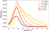 |
Fig. 1. Total SFRD in M⊙ Mpc−3 yr−1 versus redshift (z) for the six metallicity bins for the MZ19 SFRD model. |
Apart from the distribution over metallicity, the different variations, that sample some of the most important uncertainties in the observational constraints as discussed in the series of papers, also vary in the total SFRD over cosmic time. That directly translates in a different total numbers of stars formed. In Fig. 2, we show the total SFRD for the five models mentioned above, plus the Madau & Dickinson (2014) model used in SN24. It is clear that the low-metallicity models also have lower total SFRD and that the addition of starbursts adds a significant amount of star formation leading to SFRDs (which may be a factor of 2 larger than those without starbursts).
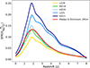 |
Fig. 2. Total SFRD in M⊙ Mpc−3 yr−1 versus redshift (z), for the six different SFRD models. The red line represents the Madau & Dickinson (2014) model used in SN24. The other five lines represent five of the SFRD models introduced in Chruślińska & Nelemans (2019), Chruślińska et al. (2020, 2021). The bottom three models are the low-, intermediate-, and high-metallicity extremes without starbursts and the top two the extreme models including starbursts (see text for more details). |
2.3. Binary population models
When we can use metallicity-dependent SFRDs we need access to binary population models that are metallicity-dependent. We also studied four different binary populations that differ in their treatment of the common-envelope phase, which plays an important role in producing close double WDs.
All the models were calculated with the SeBa population synthesis code (Portegies Zwart & Verbunt 1996; Nelemans et al. 2001b; Toonen et al. 2012) that was also used by SN24 and to make synthetic models for the population of double WDs detectable by LISA in the Galaxy and nearby galaxies (Nelemans et al. 2001a; Korol et al. 2020; Keim et al. 2023) used for LISA data challenges (Baghi 2022).
For each of the binary models we run the code for six different metallicities, to cover the bins we split the SFRD up in above: Z = 0.0001, 0.001, 0.005, 0.01, 0.02, and 0.03. For each run, we simulated 250,000 binaries with primary masses between 0.8 and 11 M⊙, distributed according to the Kroupa (2001) initial mass function, with a flat mass ratio distribution and initial separations flat in log a. Taking into account the whole mass range (i.e. also those not simulated in detail) and a mass-dependent binary fraction (based on Moe & Di Stefano 2017; van Haaften et al. 2013), this corresponds to a total mass of star formation of 3.4 × 10⁶ M⊙.
For the formation of double WDs, one of the most important uncertainties is the effect of the two mass-transfer phases on the orbit. Because the stars typically start mass transfer when the donor has a deep convective envelope, the mass transfer is assumed to be unstable (e.g. Han 1998 but see Temmink et al. 2023). Earlier studies have suggested that the standard energy-balance (α) common-envelope cannot be a good description of the first phase of mass transfer since it inevitably leads to double WDs in which the last formed WD has a lower mass, which is not observed, but that a criterion based on angular momentum balance (γ) fits better (see Toonen et al. 2012; Nelemans & Tout 2005; Nelemans et al. 2001b). Some works have suggested the first mass transfer is in fact stable (Woods et al. 2012; Li et al. 2023), but that assumption leads to the opposite situation in which the last formed WD is the more massive one, which is also not always the case. In the classical common-envelope description, α nominally represents the efficiency with which orbital energy is used to unbind the envelope; namely, with a strict upper bound on α of 1. However, the common-envelope phase is complicated and additional energy sources may be available, potentially leading to higher values. Indeed reconstruction of double WD evolution, suggests values as high as 4 (assuming a structure parameter λ = 0.5, see e.g. Nelemans & Tout 2005).
We ran two models for αα, assuming the standard common envelope in all cases with a structure parameter λ = 0.5, one with α = 1 and one with α = 4. We also ran two models for γα, assuming the first mass transfer is described by γ = 1.75 and the second common envelope either by α = 1 or by α = 4. The latter we consider our standard model.
In Fig. 3, we show the initial distribution of double WDs for this standard model as a function of initial GW frequency and chirp mass for the six different metallicities. Apart from the lowest metallicity, the bulk of the population is concentrated at low chirp mass and frequencies just above the line that indicates significant orbital evolution in a Hubble time. The lowest metallicity looks different because at low metallicity the stars are more compact leading to more massive cores when stars interact. This leads to higher chirp masses, but (more importantly) after the first mass transfer, it can also lead to tighter orbits, meaning that in the second mass transfer, the system will merge. Alternatively, in the case of more compact stars, the first mass transfer ends up avoiding the first giant branch, leading to wider systems and, eventually, to wider final orbits. The distribution changes only gradually with the metallicity. For the other models, the distributions are shown in Appendix A. They all have similar average chirp masses around 0.45 M⊙, with slightly higher values for the lowest metallicities.
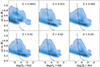 |
Fig. 3. Density plot of the initial properties of the WD population in the case of a γα, α = 4 population model: chirp mass, ℳ, versus GW frequency at the time of formation. Each panel shows a different metallicity of the Universe. The dashed lines indicate frequencies above which there is significant (10%) frequency evolution in a Hubble time. |
3. Results
Figures shown in this section all show the population model γα with α = 4, unless stated otherwise.
3.1. The effect of metallicity
We first looked at the influence of metallicity on the WD component of the AGWB in an artificial way by simulating the AGWB assuming all star formation is at a particular metallicity. The result is shown in Fig. 4, where the green and the blue line represent the estimate for the binary black hole (BBH) and binary neutron star (BNS) component (see Abbott et al. 2023), and the dark red to yellow signals represent the WD component of the AGWB for the six different metallicities, respectively. The SFRD introduced in Madau & Dickinson (2014) is used for each of the metallicities. It is clear that a metallicity of 0.0001 leads to the lowest signal, whereas a metallicity of 0.005 leads to the highest signal. The other four metallicities are indistinguishable. The difference between the various signals, coming from the use of different metallicities, is approximately a factor of 1.9 at a frequency of 1 mHz. However, all six different metallicities lead to a WD component of the AGWB that is clearly dominant over the BBH and BNS components of the AGWB. Figure 4 shows the results for a population model of γα with α = 4. The three other population models are shown in Appendix A.
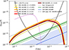 |
Fig. 4. WD components of the AGWB for six different metallicities, compared to the LVK results (upper limit to BH/NS AGWB (dashed grey Abbott et al. 2021) and estimates for the BBH and BNS components in green and blue, Abbott et al. 2023), the LISA Powerlaw Integrated sensitivity (black Thrane & Romano 2013; Alonso et al. 2020), and an estimate of the Galactic foreground (pink) based on Karnesis et al. (2021). The population synthesis model used is γα, α = 4 and the SFRD model used is that of Madau & Dickinson (2014). |
3.2. The effect of different SFRD models
In reality, the star formation is distributed over different metallicities. We show the effect of different SFRD models in Figs. 5 and 6, where the standard components are the same as those shown in Fig. 4. In Fig. 5, the dark red to yellow signals again represent the WD component of the AGWB for the six different metallicities, only this time, the MZ19 SFRD model by Chruślińska & Nelemans (2019) was used. Moreover, the SFRD was binned in the six metallicity bins, instead of using the total SFRD (as done in Fig. 4). The light green line represents the sum of all six WD components of the AGWB. Figure 5 shows that the highest and the lowest metallicity lead to the weakest AGWB signal. This is as expected, since these metallicities have lower total SFRDs in their respective bins (as shown in Fig. 1). Similarly, the metallicities leading to the highest AGWB signals, Z = 0.005, Z = 0.01, and Z = 0.02, are also related to the bins that encompass the highest total SFRDs (as also shown in Fig. 1).
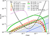 |
Fig. 5. Same details as in Fig. 4, but with the MZ19 SFRD model. The dashed lines are the WD components of the AGWB for each of the six metallicity bins, while the solid light green line is the sum of all six separate WD components. |
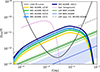 |
Fig. 6. Same details as in Fig. 4. Each line represents the sum of the signal for a different SFRD model. The light green line is the same as the one in Fig. 5. |
We plot the light green line from Fig. 5 again in Fig. 6 to illustrate the effect of the usage of different SFRD models. The five different SFRD models are clearly ordered in the same way as in Fig. 2, where the inclusion of starburst galaxies leads to higher AGWB signals than when starburst galaxies are omitted. Again, it is evident that the components of the AGWB attributed to double WDs lead to higher signals than the AGWB due to BBHs and BNSs.
The usage of these five different SFRD models leads to a factor difference in the strength of the AGWB signal of about 2.6 at 1 mHz. This suggests that using different SFRD models has a larger effect on the strength of the AGWB signal, compared to using different metallicities.
3.3. The effect of different population models
After investigating the effect of both metallicity and SFRD model, we also look at the effect of using a different population model. Up until now, the results were only shown for one single population model; namely, γα, with α = 4. Figure 7 (where the standard components are again the same as in Fig. 4) shows the effect of the usage of different population models. The light green signal (as in previous figures) represents the previously used model, γα, with α = 4. The other three signals represent each of the other three population models, respectively.
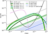 |
Fig. 7. Same details as in Fig. 4. Each line represents a different choice for population synthesis model. The MZ19 SFRD model is used. |
It is clear to see that a population model with αα, with α = 1, leads to the lowest AGWB signal due to merging double WDs. This can be explained by the fact that a lower value for α leads to a tighter orbit. This means that there are more systems in this model that merge before the second common-envelope phase occurs, which explains the low AGWB signal compared to the other three population models. The other three signals are almost indistinguishable from each other, with the model of γα, with α = 4, leading to a slightly lower signal than the other two models. There is a factor difference of roughly 2 between the highest and lowest AGWB signal at a frequency of 1 mHz, coming from using a different population model. However, it should be noted that previous research (see Sect. 2) has shown that γα, with α = 4, shows the most agreement with observations of double WDs.
3.4. Estimation of the AGWB
We show the final results of this work in Fig. 8 (where the standard components are the same as in Fig. 4). The red line shows the results from the previous work as shown in SN24. In that work, a population model of αα with α = 4 and a metallicity of 0.02, as well as the SFRD by Madau & Dickinson (2014) were used. The light green corresponds to the WD component of the AGWB for our standard model γα with α = 4 and the MZ19 SFRD model. The light green band around the AGWB signal represents the uncertainties that arose in this work. We find these uncertainties by determining the upper and lower limits of the AGWB signal at all frequencies that come from the use of the different metallicity-dependent SFRD models combined with all four binary population models. We find a strength of the WD component of the AGWB at 1 mHz of  . Just before the turnover, at a frequency of about 7 mHz, we find the following results:
  . Looking at the factor between the upper and lower limits of the AGWB signal at 1 mHz and 7 mHz, respectively, we find a difference of a factor of approximately 5 between the upper and the lower limits. We also show the normal LISA sensitivity, which is above the WD AGWB, to make it clear that the WD AGWB does not significantly impact the other LISA science.
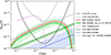 |
Fig. 8. Same details as in Fig. 4. The red line represents the WD component of the AGWB for a choice of αα, α = 4, with Z = 0.02 and the SFRD of Madau & Dickinson (2014), which is the result from SN24. The light green line represents the WD component of the AGWB for a choice of γα, α = 4 with the MZ19 SFRD model. The light green band represents the uncertainty estimate. The solid grey line shows the normal LISA sensitivity (i.e. not integrated over time and frequency). |
We find that the AGWB is comprised of approximately 2.44 × 10¹⁷ binaries, which is roughly in agreement with SN24 (who find approximately 1.5 × 10¹⁷ binaries). Moreover, we also find a similar redshift contribution as the one found in SN24, with most of the signal originating at redshifts smaller than 1.
As in SN24 we make a fit to the resulting WD AGWB. The new standard result has very similar shape so we can use the same broken broken power law with an exponential cutoff:
![Mathematical equation: $$ \begin{aligned} \Omega _{\rm GW}(f) = A\,\left(\frac{f}{\hat{f}}\right)^{0.741} \left[1 + \left(\frac{f}{\hat{f}}\right)^{4.15}\right]^{-0.255} \cdot \exp \left(-B f^3\right), \end{aligned} $$](/articles/aa/full_html/2024/11/aa51510-24/aa51510-24-eq4.gif) (2)
(2)
with different powers in the equation and different parameters: A = 1.72 × 10⁻¹¹, B = 1.54 × 10⁴ and  mHz. In Fig. 9, we plot the signal in the region above 0.3 mHz divided by a pure f2/3 power law normalised around 1 mHz, showing a similar deviation from the expected f2/3 signal, as reported in SN24. The bottom panel shows the residuals of the signal with respect to the fit, which remain below 2%.
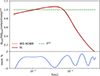 |
Fig. 9. Comparison of the WD AGWB (salmon) and the broken power law fit (dark red) to a purely f2/3 signal (green dashed) by dividing the curves by f2/3. The WD AGWB deviates from the expected 2/3 slope, but residuals (bottom) between the WD AGWB and the fit are below 2%. |
4. Discussion and conclusions
In this study, we have explored some of the factors that introduce an uncertainty in the expected level and shape of the WD AGWB. Although this gives a good indication of the range of possibilities that are definitely possible, it is not an exhaustive study of all the possible effects. For the SFRD models, the extensive survey of the existing observational evidence carried out by Chruślińska & Nelemans (2019) and Chruślińska et al. (2020, 2021) implies that the largest uncertainties are in fact captured by the different models we use. However, for the binary population models this is less clear. The large number of uncertain phases in the evolution of binaries makes a quantitative assessment of the uncertainties difficult. We also neglected the possibility that metallicity also changes the initial binary parameters (Badenes et al. 2018; Moe et al. 2019). Comparison of the same binary models with the very local population of double WDs in the solar neighbourhood (e.g. Nelemans et al. 2001b; Toonen et al. 2012) suggests that at least at approximately solar metallicity, the models are not too far off; however, whether this means a factor 3 or a factor 5 is unclear.
We compare our main results to the results in Farmer & Phinney (2003) and SN24. They find values for ΩWD at a frequency of 1 mHz of: ΩWD(1 mHz) = 3.57 × 10⁻¹² and ΩWD(1 mHz) = 5.7 × 10⁻¹², respectively. We find ΩWD(1 mHz) = 4.01 × 10⁻¹². This difference is not unexpected, since the WD component of the AGWB (as shown in Fig. 8) shows the result of SN24 above the result of this work. Possible explanations for the differences between Farmer & Phinney (2003) and SN24 are described in the latter. Differences between this work and SN24 can be explained by both the usage of a different population model as well as a different SFRD model.
There are some simplifications that we make in the calculation, in particular, about the population of sources that give rise to the AGWB being completely isotropic. At large redshifts this is very likely completely justified, but as a significant contribution to the signal originates within the volume smaller than z = 0.5, the total signal will be anisotropic since the mass distribution in the Universe is highly structured. It would be interesting to calculate the level of anisotropy and the ability of the LISA measurements to detect this property (see Cusin et al. 2018).
The other question is whether LISA can detect the turnover of the WD AGWB around 10 mHz, which seems likely given the sensitivity curve, but it is also useful to consider how well the shape of the turnover can be characterised. An even more interesting aspect would certainly be the detection of the second turnover around 50 mHz, where the BH AGWB is expected to become dominant over the WD AGWB.
In conclusion, we have investigated the influence of metallicity, different star formation estimates across cosmic time and different descriptions of the common-envelope phase on the level and shape of the WD AGWB. We conclude that the metallicity does not significantly impact the results, since only the very lowest metallicity (Z = 0.0001) produces a lower signal. However, the uncertainties in the (total amount) of star formation give rise to an significant uncertainty in the level of the signal, while different binary populations have less of an effect on the level; however, the uncertainties also influence the shape of the turnover of the signal. The total uncertainty on the level of the signal is about a factor of 5. The uncertainty in the model suggests the detection of the signal by a future GW detector would provide information about the star formation history and the binary properties at significant redshifts. The uncertainties are not large enough to challenge the conclusion that in the mHz regime, the AGWB is dominated by the WD population to a level that is significantly above the contribution of BHs.
Acknowledgments
We thank Seppe Staelens for his earlier work, discussions and help and the referee for valuable suggestions and comments. G.N. is supported by the Dutch science foundation NWO.
References
- Abbott, R., Abbott, T. D., Abraham, S., et al. 2021, Phys. Rev. D, 104, 022004 [NASA ADS] [CrossRef] [Google Scholar]
- Abbott, R., Abbott, T. D., Acernese, F., et al. 2023, Phys. Rev. X, 13, 011048 [NASA ADS] [Google Scholar]
- Acernese, F., Agathos, M., Agatsuma, K., et al. 2015, Class. Quant. Grav., 32, 024001 [Google Scholar]
- Alonso, D., Contaldi, C. R., Cusin, G., Ferreira, P. G., & Renzini, A. I. 2020, Phys. Rev. D, 101, 124048 [NASA ADS] [CrossRef] [Google Scholar]
- Amaro-Seoane, P., Audley, H., Babak, S., et al. 2017, ArXiv e-prints [arXiv:1702.00786] [Google Scholar]
- Amaro-Seoane, P., Andrews, J., Arca Sedda, M., et al. 2023, Liv. Rev. Relat., 26, 2 [NASA ADS] [CrossRef] [Google Scholar]
- Aso, Y., Michimura, Y., Somiya, K., et al. 2013, Phys. Rev. D, 88, 043007 [NASA ADS] [CrossRef] [Google Scholar]
- Auclair, P., Bacon, D., Baker, T., et al. 2023, Liv. Rev. Relat., 26, 5 [NASA ADS] [CrossRef] [Google Scholar]
- Babak, S., Caprini, C., Figueroa, D. G., et al. 2023, JCAP, 2023, 034 [CrossRef] [Google Scholar]
- Badenes, C., Mazzola, C., Thompson, T. A., et al. 2018, ApJ, 854, 147 [NASA ADS] [CrossRef] [Google Scholar]
- Baghi, Q. 2022, ArXiv e-prints [arXiv:2204.12142] [Google Scholar]
- Bavera, S. S., Franciolini, G., Cusin, G., et al. 2022, A&A, 660, A26 [NASA ADS] [CrossRef] [EDP Sciences] [Google Scholar]
- Binétruy, P., Bohé, A., Caprini, C., & Dufaux, J.-F. 2012, JCAP, 2012, 027 [Google Scholar]
- Caprini, C., & Figueroa, D. G. 2018, Class. Quant. Grav., 35, 163001 [NASA ADS] [CrossRef] [Google Scholar]
- Caprini, C., Durrer, R., & Servant, G. 2009, JCAP, 2009, 024 [CrossRef] [Google Scholar]
- Chruślińska, M., & Nelemans, G. 2019, MNRAS, 488, 5300 [CrossRef] [Google Scholar]
- Chruslinska, M., Belczynski, K., Klencki, J., & Benacquista, M. 2018, MNRAS, 474, 2937 [CrossRef] [Google Scholar]
- Chruślińska, M., Jeřábková, T., Nelemans, G., & Yan, Z. 2020, A&A, 636, A10 [NASA ADS] [CrossRef] [EDP Sciences] [Google Scholar]
- Chruślińska, M., Nelemans, G., Boco, L., & Lapi, A. 2021, MNRAS, 508, 4994 [CrossRef] [Google Scholar]
- Cusin, G., Dvorkin, I., Pitrou, C., & Uzan, J.-P. 2018, Phys. Rev. Lett., 120, 231101 [CrossRef] [Google Scholar]
- Dvorkin, I., Vangioni, E., Silk, J., Uzan, J.-P., & Olive, K. A. 2016, MNRAS, 461, 3877 [CrossRef] [Google Scholar]
- Evans, C. R., Iben, I., Smarr, L., et al. 1987, ApJ, 323, 129 [NASA ADS] [CrossRef] [Google Scholar]
- Farmer, A. J., & Phinney, E. S. 2003, MNRAS, 346, 1197 [NASA ADS] [CrossRef] [Google Scholar]
- Giacobbo, N., & Mapelli, M. 2018, MNRAS, 480, 2011 [Google Scholar]
- Han, Z. 1998, MNRAS, 296, 1019 [NASA ADS] [CrossRef] [Google Scholar]
- Hils, D., Bender, P. L., & Webbink, R. F. 1990, ApJ, 360, 75 [CrossRef] [Google Scholar]
- Karnesis, N., Babak, S., Pieroni, M., Cornish, N., & Littenberg, T. 2021, Phys. Rev. D, 104, 043019 [NASA ADS] [CrossRef] [Google Scholar]
- Keim, M. A., Korol, V., & Rossi, E. M. 2023, MNRAS, 521, 1088 [NASA ADS] [CrossRef] [Google Scholar]
- Korol, V., Toonen, S., Klein, A., et al. 2020, A&A, 638, A153 [NASA ADS] [CrossRef] [EDP Sciences] [Google Scholar]
- Korol, V., Hallakoun, N., Toonen, S., & Karnesis, N. 2022, MNRAS, 511, 5936 [NASA ADS] [CrossRef] [Google Scholar]
- Kowalska-Leszczynska, I., Regimbau, T., Bulik, T., Dominik, M., & Belczynski, K. 2015, A&A, 574, A58 [NASA ADS] [CrossRef] [EDP Sciences] [Google Scholar]
- Kroupa, P. 2001, MNRAS, 322, 231 [NASA ADS] [CrossRef] [Google Scholar]
- Lamberts, A., Blunt, S., Littenberg, T. B., et al. 2019, MNRAS, 490, 5888 [NASA ADS] [CrossRef] [Google Scholar]
- Lehoucq, L., Dvorkin, I., Srinivasan, R., Pellouin, C., & Lamberts, A. 2023, MNRAS, 526, 4378 [NASA ADS] [CrossRef] [Google Scholar]
- Li, Z., Chen, X., Ge, H., Chen, H.-L., & Han, Z. 2023, A&A, 669, A82 [NASA ADS] [CrossRef] [EDP Sciences] [Google Scholar]
- LIGO Scientific Collaboration (Aasi, J., et al.) 2015, Class. Quant. Grav., 32, 074001 [Google Scholar]
- Lipunov, V. M., Postnov, K. A., & Prokhorov, M. E. 1987, A&A, 176, L1 [NASA ADS] [Google Scholar]
- Luo, J., Chen, L.-S., Duan, H.-Z., et al. 2016, Class. Quant. Grav., 33, 035010 [NASA ADS] [CrossRef] [Google Scholar]
- Luo, Z., Wang, Y., Wu, Y., Hu, W., & Jin, G. 2021, Progr. Theor. Exp. Phys., 2021, 05A108 [CrossRef] [Google Scholar]
- Madau, P., & Dickinson, M. 2014, ARA&A, 52, 415 [Google Scholar]
- Moe, M., & Di Stefano, R. 2017, ApJS, 230, 15 [Google Scholar]
- Moe, M., Kratter, K. M., & Badenes, C. 2019, ApJ, 875, 61 [NASA ADS] [CrossRef] [Google Scholar]
- Neijssel, C. J., Vigna-Gómez, A., Stevenson, S., et al. 2019, MNRAS, 490, 3740 [Google Scholar]
- Nelemans, G., & Tout, C. A. 2005, MNRAS, 356, 753 [NASA ADS] [CrossRef] [Google Scholar]
- Nelemans, G., Yungelson, L. R., & Portegies Zwart, S. F. 2001a, A&A, 375, 890 [NASA ADS] [CrossRef] [EDP Sciences] [Google Scholar]
- Nelemans, G., Yungelson, L. R., Portegies Zwart, S. F., & Verbunt, F. 2001b, A&A, 365, 491 [NASA ADS] [CrossRef] [EDP Sciences] [Google Scholar]
- Nissanke, S., Vallisneri, M., Nelemans, G., & Prince, T. A. 2012, ApJ, 758, 131 [NASA ADS] [CrossRef] [Google Scholar]
- Phinney, E. S. 2001, ArXiv e-prints [arXiv:astro-ph/0108028] [Google Scholar]
- Portegies Zwart, S. F., & Verbunt, F. 1996, A&A, 309, 179 [NASA ADS] [Google Scholar]
- Ruiter, A. J., Belczynski, K., Benacquista, M., Larson, S. L., & Williams, G. 2010, ApJ, 717, 1006 [NASA ADS] [CrossRef] [Google Scholar]
- Schneider, R., Ferrari, V., Matarrese, S., & Portegies Zwart, S. F. 2001, MNRAS, 324, 797 [NASA ADS] [CrossRef] [Google Scholar]
- Staelens, S., & Nelemans, G. 2024, A&A, 683, A139 [NASA ADS] [CrossRef] [EDP Sciences] [Google Scholar]
- Temmink, K. D., Pols, O. R., Justham, S., Istrate, A. G., & Toonen, S. 2023, A&A, 669, A45 [NASA ADS] [CrossRef] [EDP Sciences] [Google Scholar]
- Thrane, E., & Romano, J. D. 2013, Phys. Rev. D, 88, 124032 [NASA ADS] [CrossRef] [Google Scholar]
- Toonen, S., Nelemans, G., & Portegies Zwart, S. 2012, A&A, 546, A70 [NASA ADS] [CrossRef] [EDP Sciences] [Google Scholar]
- van Haaften, L. M., Nelemans, G., Voss, R., et al. 2013, A&A, 552, A69 [NASA ADS] [CrossRef] [EDP Sciences] [Google Scholar]
- Woods, T. E., Ivanova, N., van der Sluys, M. V., & Chaichenets, S. 2012, ApJ, 744, 12 [NASA ADS] [CrossRef] [Google Scholar]
- Yu, S., & Jeffery, C. S. 2013, MNRAS, 429, 1602 [CrossRef] [Google Scholar]
Appendix A: Additional figures
In this appendix we provide additional figures that give more details on the different models.
Firstly, in the main paper we present the split of the SFRD over six different metallicity bins for the MZ19 model in Fig. 1. Figures A.1 and Fig. A.2 give the same for the LZ21 and the HZ21 SFRD models. The LZ19 and HZ19 SFRD model are left out, since these are very similar except for the normalisation due to the inclusion of starburst galaxies in the new models.
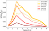 |
Fig. A.1. Total SFRD versus redshift (z), for the six metallicity bins for the LZ21 SFRD model. |
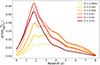 |
Fig. A.2. Total SFRD versus redshift (z), for the six metallicity bins for the HZ21 SFRD model. |
In the main text, we present the results for our default binary evolution model (γα, with α = 4). Figures A.6 to A.8 show the initial GW frequency and chirp mass for the different metallicities for the population models αα, with α = 1, αα, with α = 4 and γα, with α = 1, respectively. As for the standard model, most metallicities show very similar structure with gradual changes, mostly towards lower GW frequency and higher chirp mass for lower metallicity, with the lowest metallicity model often being quite different. As for the standard model, this is mostly due to the fact that stars are more compact at low metallicity.
The resulting AGWB spectra for the hypothetical cases that all star formation would happen at a single metallicity are shown in Fig. A.3 to A.5. These are the same as Fig. 4, except for the other population models. For the αα, with α = 1 model the shorter periods after the common envelope lead to an increasing number of sources with higher chirp mass towards lower metallicity, making the lower metallicity AGWBs higher than those of higher metallicity. This is contrary to in our standard model, but the overall AGWB is lower in these models. The αα, with α = 4 model shows similar behaviour to the standard model, with somewhat higher overall levels. Finally, in the γα, with α = 1 model, the increase in chrip mass towards lower metallicity is compensated with decrease in over all number, leading to very similar overall AGWB levels for all metallicities.
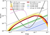 |
Fig. A.3. Same details as in Fig. 4. The population synthesis model used is αα, α = 1 and the SFRD used is that of Madau & Dickinson (2014). |
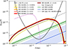 |
Fig. A.4. Same details as in Fig. 4. The population synthesis model used is αα, α = 4 and the SFRD used is that of Madau & Dickinson (2014). |
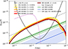 |
Fig. A.5. Same details as in Fig. 4. The population synthesis model used is γα, α = 1 and the SFRD used is that of Madau & Dickinson (2014). |
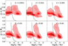 |
Fig. A.6. Density plot of the initial properties of the WD population in the case of a αα, α = 1 population synthesis model: chirp mass, ℳ, versus GW frequency at the time of formation. Each panel shows a different metallicity of the universe. The dashed lines indicate frequencies above which there is significant (10%) frequency evolution in a Hubble time. |
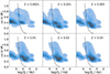 |
Fig. A.7. Density plot of the initial properties of the WD population in the case of a αα, α = 4 population synthesis model: chirp mass, ℳ, versus GW frequency at the time of formation. Each panel shows a different metallicity of the universe. The dashed lines indicate frequencies above which there is significant (10%) frequency evolution in a Hubble time. |
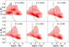 |
Fig. A.8. Density plot of the initial properties of the WD population in the case of a γα, α = 1 population synthesis model: chirp mass, ℳ, versus GW frequency at the time of formation. Each panel shows a different metallicity of the universe. The dashed lines indicate frequencies above which there is significant (10%) frequency evolution in a Hubble time. |
All Figures
|
Fig. 1. Total SFRD in M⊙ Mpc−3 yr−1 versus redshift (z) for the six metallicity bins for the MZ19 SFRD model. |
| In the text | |
|
Fig. 2. Total SFRD in M⊙ Mpc−3 yr−1 versus redshift (z), for the six different SFRD models. The red line represents the Madau & Dickinson (2014) model used in SN24. The other five lines represent five of the SFRD models introduced in Chruślińska & Nelemans (2019), Chruślińska et al. (2020, 2021). The bottom three models are the low-, intermediate-, and high-metallicity extremes without starbursts and the top two the extreme models including starbursts (see text for more details). |
| In the text | |
|
Fig. 3. Density plot of the initial properties of the WD population in the case of a γα, α = 4 population model: chirp mass, ℳ, versus GW frequency at the time of formation. Each panel shows a different metallicity of the Universe. The dashed lines indicate frequencies above which there is significant (10%) frequency evolution in a Hubble time. |
| In the text | |
|
Fig. 4. WD components of the AGWB for six different metallicities, compared to the LVK results (upper limit to BH/NS AGWB (dashed grey Abbott et al. 2021) and estimates for the BBH and BNS components in green and blue, Abbott et al. 2023), the LISA Powerlaw Integrated sensitivity (black Thrane & Romano 2013; Alonso et al. 2020), and an estimate of the Galactic foreground (pink) based on Karnesis et al. (2021). The population synthesis model used is γα, α = 4 and the SFRD model used is that of Madau & Dickinson (2014). |
| In the text | |
|
Fig. 5. Same details as in Fig. 4, but with the MZ19 SFRD model. The dashed lines are the WD components of the AGWB for each of the six metallicity bins, while the solid light green line is the sum of all six separate WD components. |
| In the text | |
|
Fig. 6. Same details as in Fig. 4. Each line represents the sum of the signal for a different SFRD model. The light green line is the same as the one in Fig. 5. |
| In the text | |
|
Fig. 7. Same details as in Fig. 4. Each line represents a different choice for population synthesis model. The MZ19 SFRD model is used. |
| In the text | |
|
Fig. 8. Same details as in Fig. 4. The red line represents the WD component of the AGWB for a choice of αα, α = 4, with Z = 0.02 and the SFRD of Madau & Dickinson (2014), which is the result from SN24. The light green line represents the WD component of the AGWB for a choice of γα, α = 4 with the MZ19 SFRD model. The light green band represents the uncertainty estimate. The solid grey line shows the normal LISA sensitivity (i.e. not integrated over time and frequency). |
| In the text | |
|
Fig. 9. Comparison of the WD AGWB (salmon) and the broken power law fit (dark red) to a purely f2/3 signal (green dashed) by dividing the curves by f2/3. The WD AGWB deviates from the expected 2/3 slope, but residuals (bottom) between the WD AGWB and the fit are below 2%. |
| In the text | |
|
Fig. A.1. Total SFRD versus redshift (z), for the six metallicity bins for the LZ21 SFRD model. |
| In the text | |
|
Fig. A.2. Total SFRD versus redshift (z), for the six metallicity bins for the HZ21 SFRD model. |
| In the text | |
|
Fig. A.3. Same details as in Fig. 4. The population synthesis model used is αα, α = 1 and the SFRD used is that of Madau & Dickinson (2014). |
| In the text | |
|
Fig. A.4. Same details as in Fig. 4. The population synthesis model used is αα, α = 4 and the SFRD used is that of Madau & Dickinson (2014). |
| In the text | |
|
Fig. A.5. Same details as in Fig. 4. The population synthesis model used is γα, α = 1 and the SFRD used is that of Madau & Dickinson (2014). |
| In the text | |
|
Fig. A.6. Density plot of the initial properties of the WD population in the case of a αα, α = 1 population synthesis model: chirp mass, ℳ, versus GW frequency at the time of formation. Each panel shows a different metallicity of the universe. The dashed lines indicate frequencies above which there is significant (10%) frequency evolution in a Hubble time. |
| In the text | |
|
Fig. A.7. Density plot of the initial properties of the WD population in the case of a αα, α = 4 population synthesis model: chirp mass, ℳ, versus GW frequency at the time of formation. Each panel shows a different metallicity of the universe. The dashed lines indicate frequencies above which there is significant (10%) frequency evolution in a Hubble time. |
| In the text | |
|
Fig. A.8. Density plot of the initial properties of the WD population in the case of a γα, α = 1 population synthesis model: chirp mass, ℳ, versus GW frequency at the time of formation. Each panel shows a different metallicity of the universe. The dashed lines indicate frequencies above which there is significant (10%) frequency evolution in a Hubble time. |
| In the text | |
Current usage metrics show cumulative count of Article Views (full-text article views including HTML views, PDF and ePub downloads, according to the available data) and Abstracts Views on Vision4Press platform.
Data correspond to usage on the plateform after 2015. The current usage metrics is available 48-96 hours after online publication and is updated daily on week days.
Initial download of the metrics may take a while.