| Issue |
A&A
Volume 683, March 2024
|
|
|---|---|---|
| Article Number | A139 | |
| Number of page(s) | 6 | |
| Section | Extragalactic astronomy | |
| DOI | https://doi.org/10.1051/0004-6361/202348429 | |
| Published online | 15 March 2024 | |
Likelihood of white dwarf binaries to dominate the astrophysical gravitational wave background in the mHz band
1
Institute of Astronomy, KU Leuven, Celestijnenlaan 200D, 3001 Leuven, Belgium
2
Department of Astrophysics/IMAPP, Radboud University PO Box 9010 6500 GL Nijmegen, The Netherlands
3
DAMTP, Centre for Mathematical Sciences, University of Cambridge, Wilberforce Road, Cambridge CB3 0WA, UK
e-mail: This email address is being protected from spambots. You need JavaScript enabled to view it.
4
SRON, Netherlands Institute for Space Research, Niels Bohrweg 4, 2333 CA Leiden, The Netherlands
Received:
30
October
2023
Accepted:
8
December
2023
Abstract
Context. The astrophysical gravitational wave background (AGWB) is a collective signal of astrophysical gravitational wave sources dominated by compact binaries. One key science goal of current and future gravitational wave detectors is to obtain its measurement.
Aims. We aim to determine the population of compact binaries dominating the AGWB in the mHz band. We revisit and update an earlier work by Farmer & Phinney (2003, MNRAS, 346, 1197) to model the astrophysical gravitational wave background sourced by extragalactic white dwarf binaries in the mHz frequency band.
Methods. We calculated the signal using a single-metallicity model for the white dwarf population in the Universe using the global star formation history.
Results. We estimate the white dwarf AGWB amplitude to be ∼60% higher than the earlier estimate. We also find that the overall shape of the white dwarf AGWB shows a good fit with a broken power law combined with an exponential cut-off.
Conclusions. We compare our results to present-day best estimates for the background due to black hole and neutron star binaries, finding that the white dwarf component is likely to dominate in the mHz band. We provide an order-of-magnitude estimate that explains this hierarchy and we comment on the implications for future missions that aim to detect the AGWB. We also note that the black hole AGWB may only be detectable at high frequency. We outline several improvements that can be made to our estimate, however, these points are unlikely to change our main conclusion, which posits that the white dwarf AGWB dominates the mHz band.
Key words: gravitation / gravitational waves / binaries: close / stars: black holes / white dwarfs
© The Authors 2024
 Open Access article, published by EDP Sciences, under the terms of the Creative Commons Attribution License (https://creativecommons.org/licenses/by/4.0), which permits unrestricted use, distribution, and reproduction in any medium, provided the original work is properly cited.
This article is published in open access under the Subscribe to Open model. This email address is being protected from spambots. You need JavaScript enabled to view it. to support open access publication.
1. Introduction
Apart from individual gravitational wave (GW) sources, such as the black hole (BH) and neutron star (NS) mergers detected by the LIGO/Virgo/Kagra (LVK) collaboration (Abbott et al. 2023a) in the relatively nearby Universe, there is an isotropic stochastic signal coming from all GW-emitting sources in the Universe (e.g., Schneider et al. 2010; Christensen 2019). In particular, all compact binaries that are evolving due to the emission of GW form a signal that displays a characteristic spectral shape (Phinney 2001) and this is generally referred to as the astrophysical GW background (denoted as AGWB to distinguish it from potential stochastic GW signals originating in the Early Universe, e.g., Schneider et al. 2001; Farmer & Phinney 2003; Kowalska-Leszczynska et al. 2015; Amaro-Seoane et al. 2023). It is a broadband signal that extends from the high-frequency band covered by the LVK detectors to the mHz band, which will be covered by future space GW detectors such as LISA (Amaro-Seoane et al. 2017), Taiji (Luo et al. 2021), and TianQin (Luo et al. 2016).
Although the AGWB is a collective signal, it provides information on the global properties of the population of compact binaries that are not individually detectable because they are too far away for their intrinsic luminosity. Following the discovery that the binary BH (BBH) population is both greater and contains more massive BH than previously believed (see Abbott et al. 2016), several investigations have calculated the expected AGWB caused by BBHs (and binary neutrons stars, BNSs, e.g., Dvorkin et al. 2016; Bavera et al. 2022; Babak et al. 2023; Lehoucq et al. 2023). These studies concluded that it would be detectable by the LISA mission and future ground based detectors such as Einstein Telescope (Punturo et al. 2010) and Cosmic Explorer (Reitze et al. 2019).
A more detailed understanding of the AGWB is also necessary to fully characterise and remove it from the data to uncover underlying signals, such as GWs from the Early Universe, which have become an increasingly popular research topic (see e.g., Caprini et al. 2009; Binétruy et al. 2012; Auclair et al. 2023), or GWs from faint individual sources.
In the mHz band, apart from BH and NS binaries, there is also a contribution from white dwarf (WD) and other binaries. Farmer & Phinney (2003) performed a detailed calculation of the AGWB excluding BH and NS systems but did not discuss in detail the notion of whether it would be detectable by the LISA mission. Meanwhile, Schneider et al. (2001) concluded that the WD AGWB would dominate. We note that due to the much larger size of WD and other stars, they do not contribute to the AGWB above frequencies of about 100 mHz (Farmer & Phinney 2003). We also stress that this WD AGWB should not be confused with the stochastic signal of unresolved WD binaries within our Milky Way, referred to as the GW ‘foreground’; although the latter is stochastic, it is far from isotropic (e.g., Edlund et al. 2005). Given the conclusion that the BH AGWB can (easily) be detected by the LISA mission (e.g., Caprini et al. 2016; Babak et al. 2023), we find that it is time to reinvestigate the relative importance of the WD AGWB.
In this paper, we compare the BH AGWB as derived from the LVK measurements with a new estimate of the WD AGWB. In Sect. 2, we describe our methods. In Sect. 3, we present our results and in Sect. 4, we discuss these results and their limitations, followed by our conclusions. We use a cosmology based on the parameters from Planck Collaboration VI (2020).
2. Methods
The AGWB is described in terms of the dimensionless energy density spectrum:
 (1)
(1)
where  is the critical density of the Universe, ℰGW is the present-day energy density in GWs and fr is the received GW frequency. In an isotropic and homogeneous Universe, the present-day GW energy density due to a population of compact binaries in the inspiral phase is given by (Phinney 2001)
 (2)
(2)
In this expression, N(z) is the number density of sources with energy spectrum  . The latter can be approximated by the leading quadrupole order of the emitted GW radiation (Hawking & Israel 1987)
 (3)
(3)
The frequency of the GW is related to the orbital frequency ν as fe = 2ν. We note that fe is the GW frequency in the rest frame of the emitting source, which is redshifted as fe = fr(1 + z) by the time the signal is detected. The limiting frequencies depend on the source properties: the lower limit, fmin, is set by the separation of the system after circularisation, and is such that the system changes frequency significantly within a Hubble time. The frequency at which the source emits increases over time as (Farmer & Phinney 2003):
 (4)
(4)
until the binary components come into Roche lobe contact or the evolution becomes dominated by tidal forces. This sets a minimal orbital separation, and therefore a maximal frequency fmax, for the binary. Equation (4) can be integrated as follows:
 (5)
(5)
where t0 and ν0 are the time and frequency of the binary at birth, respectively. The constant in Eq. (4) depends on the chirp mass as follows:
 (6)
(6)
If we allow the population to have varying chirp mass, the background is given by (Farmer & Phinney 2003; Renzini et al. 2022):
 (7)
(7)
Therefore, if the integrals do not have a frequency dependence, the expected spectral dependence of the AGWB sourced by compact binaries is:
 (8)
(8)
where fref is a reference frequency to which the background is normalised.
2.1. Estimating the AGWB
This section aims to provide an estimate of the different contributions to the compact binary AGWB in the LISA frequency band. We first focus on the contributions of the BBH and BNS signals, leaving out the NS+BH population for simplicity (and it is subdominant). These contributions are obtained by extrapolating the current best estimates in the LVK band using Eq. (8). In reality, the signal may drop off somewhat more steeply, especially at low frequencies (e.g., Schneider et al. 2001), so this extrapolation is an upper bound. The current upper limit on the AGWB in the LVK band is (Abbott et al. 2021):
 (9)
(9)
at the 95% confidence interval. The best estimates, based on current knowledge of the compact binary population are (Abbott et al. 2023b):
 (10)
(10)
 (11)
(11)
The WD contribution is obtained by updating the work of Farmer & Phinney (2003). The method we followed is based on their Sect. 6. It starts from an alternative formulation of Eq. (1):
 (12)
(12)
where  is the specific flux received from an object with specific luminosity, Lfe, at redshift, z. It is given by:
 (13)
(13)
where dL = (1 + z)dM is the luminosity distance to redshift, z, and dM is the proper motion distance. In the case of a large number of systems, all these contributions can be added together by introducing the specific luminosity density, lfe, defined as dLfe(z) = lfe(z)dV(z). Then, dV(z) is the comoving volume element at redshift z, namely, dV(z) = 4πdM(z)2dχ, with χ(z) the proper motion distance. The specific flux given in Eq. (13) can then be rewritten as:
 (14)
(14)
In order to evaluate this numerically, the integral over the redshift is discretized1 in 20 bins over the interval of z ∈ [0, 8]. Furthermore, the frequency range [10−5, 1] Hz is divided into 50 bins, and the received flux per bin is calculated as:
 (15)
(15)
where we integrated over fr and performed a change of variables as fr → fe. This expression essentially shows that we integrate over all the source frequencies that get redshifted to the correct observed frequency bin. The specific luminosity density is determined as the sum of the contributions of different systems, labeled as k, and equal to
 (16)
(16)
The luminosity is given by (Peters & Mathews 1963)
 (17)
(17)
and nk(fe, z) is the specific number density of systems of type k at redshift z, emitting GWs at a frequency fe. The specific number density scales as nk(f) = Akf−11/3 (see Eq. (23)), where the proportionality constant Ak is such that:
 (18)
(18)
with nbin(k; z) the number density of systems k at redshift z emitting GWs with frequencies in the correct bin. The latter can be estimated by multiplying the star formation rate per unit of volume, ψ, with the time it takes a binary to traverse the frequency bin:
 (19)
(19)
The factor 𝒫k reflects the proportion of the formed stars that end up in a binary with properties corresponding to label k. The value of Δz reflects an additional redshift to reflect the conditions at formation of the binary, before evolving to the frequency at the lower end of the bin, which happens at redshift z. This time delay, as well as Δt can be calculated using Eq. (5). The population model and star formation rate history that we used are explained in the next section. Finally, the energy density in the frequency bin is calculated as
 (20)
(20)
where fr is now an appropriately chosen frequency that represents the bin.
2.2. The WD population model and star formation rate history
In order to sample the population of WD in the different redshift shells, we calculated a model for the population of double WD based on the SeBa population synthesis code (Portegies Zwart & Verbunt 1996; Nelemans et al. 2001b; Toonen et al. 2012). This code also has also been used to make synthetic models for the population of double WD detectable by LISA in the Galaxy and nearby galaxies (Nelemans et al. 2001a; Korol et al. 2020; Keim et al. 2023) and used in the LISA Data Challenges (Baghi 2022). For this first estimate of the WD AGWB, we used a single (solar) metallicity and simulate 250 000 binaries with initial masses between 0.9 and 11 M⊙, distributed according to the initial mass function (IMF) of Kroupa (2001), with a flat mass ratio distribution and initial separations flat in log a. For each of the systems, the evolution was followed and we selected 14 418 systems that form a close (a < 500 R⊙) double WD. The properties with which the WD binaries are formed (chirp mass and GW frequency) are shown in Fig. 1, with the majority of sources having low chirp mass and frequencies at formation below 1 mHz, with an additional tail of systems forming with frequencies above 1 mHz.
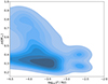 |
Fig. 1. Density plot (linear scale) of the initial properties of the WD population: chirp mass, ℳ, versus GW frequency at the time of formation. |
The population we obtained corresponds to 4 × 10⁶ M⊙ of total star formation, taking the complete IMF and the mass dependent binary fraction (Moe & Di Stefano 2017) into account. We then take this population to be representative for every redshift shell in Eq. (15). This means that we sum over all the binaries of our population in Eq. (16), and the factor 𝒫k in Eq. (19) can be replaced as follows:
 (21)
(21)
The star formation history is taken to be the one in Madau & Dickinson (2014):
![Mathematical equation: $$ \begin{aligned} \psi (z) = 0.015\frac{(1+z)^{2.7}}{1+[(1+z)/2.9]^{5.6}} \,M_\odot \,\text{ yr}^{-1}\,\text{ Mpc}^{-3}. \end{aligned} $$](/articles/aa/full_html/2024/03/aa48429-23/aa48429-23-eq25.gif) (22)
(22)
This exhibits a peak approximately 3.5 Gyr after the Big Bang, at z ≈ 1.9.
3. Results
3.1. Order of magnitude
Before we share the results of the estimate of the AGWB, we can make an order-of-magnitude estimate of the relative importance of WD, NS, and BH to the AGWB, by comparing the number density of sources as function of frequency of each of the classes and their GW luminosity. The number density of sources can easily be estimated from Eq. (4) via
 (23)
(23)
with ℛ as the rate at which systems arrive at a certain frequency. For sources that are inspiralling, ℛ can be approximated by the merger rate of the sources. The contribution to the AGWB of two sets of sources with such density is simply this number density times the signal per source (see Eq. (12)):
 (24)
(24)
where we use Eqs. (13) and (17) to estimate the flux (assuming they have the same distance distribution).
We assumed a typical chirp mass for BBH of 20 M⊙, for BNS of 1.2 M⊙ and for WD binaries of 0.3 M⊙ (components of 0.3 and 0.4 M⊙). For BBH and BNS, we estimated the merger rates in the Milky Way by scaling from the volume rates of the LVK collaboration (Abbott et al. 2023b), as in Abadie et al. (2010). We used the same method as in Nelemans et al. (2004) to obtain the merger rate of the WD population described above in the Milky Way. This results in the values given in Table 1, demonstrating that the WD background is likely to dominate, with the BH background reaching the same order of magnitude. The NS background is likely to be substantially less important.
Order-of-magnitude estimates of the AGWB using the merger rate per Milky Way equivalent galaxy (MWEG) and a typical chirp mass of WD, BH, and NS binaries.
3.2. The estimated AGWB
The resulting components of the AGWB in the mHz frequency band calculated according to the methods discussed above are shown in Fig. 2, with the LVK extrapolations in green (BBH) and blue (BNS) and the calculated WD signals in orange. It is seen that the calculated WD component is significantly larger than the BH (and NS) component – about an order of magnitude. Furthermore, it is also seen to be larger than the extrapolated upper limit in the LVK frequency band, and well above the LISA sensitivity curve in the range 10−3 − 10−2 Hz.
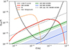 |
Fig. 2. Resulting WD component (thick salmon) of the AGWB compared to the LVK results (upper limit to BH/NS AGWB (dashed grey) and estimates for the BBH and BNS components in green and blue), the LISA Powerlaw Integrated sensitivity (black, Thrane & Romano 2013; Alonso et al. 2020), and an estimate of the Galactic foreground (brown) based on Karnesis et al. (2021). A fit to the WD component is shown in dark red. |
The WD component displays a turnover around 10 mHz and the BH component becomes dominant around 40 mHz. This can be explained due to the fact that most WD binaries have fmax ≲ 100 mHz, causing a steady decline in number of sources that can contribute to the total background signal. Below ∼0.5 mHz the WD signal also drops off, due to the fact that most of the systems form in that region and also because the merger time for the systems becomes larger than the Hubble time (see also Farmer & Phinney 2003).
The WD signal seems to follow a straight power law. In order to investigate this further, we plot in Fig. 3 the signal in the region above 0.3 mHz divided by a pure f2/3 power law normalised at 1 mHz. It is clear that there is a small deviation from a straight power law and also that the slope is slightly steeper than the expected 2/3 (Eq. (8)). The signal is fitted well by a broken power law with an exponential cutoff:
![Mathematical equation: $$ \begin{aligned} \Omega _{\rm GW} (f) = A \left(\frac{f}{\hat{f}}\right)^{0.73} \left[ 1 + \left( \frac{f}{\hat{f}} \right)^{4.1} \right]^{-0.23} \cdot \exp (-Bf^{3}) \end{aligned} $$](/articles/aa/full_html/2024/03/aa48429-23/aa48429-23-eq28.gif) (25)
(25)
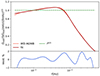 |
Fig. 3. Comparison of the WD AGWB (salmon) and the broken power law fit (dark red) to a purely f2/3 signal (green dashed) by dividing the curves by f2/3. The WD AGWB deviates from the expected 2/3 slope, but the residuals (bottom) between the WD AGWB and the fit are below 5%. |
where A = 2.4 × 10⁻¹¹, B = 1.2 × 10⁴ and  mHz. The bottom panel of Fig. 3 shows the residuals of the signal with respect to the fit, which for this simple fit remain below 2 percent. So, this fit is a good enough approximation for most studies.
Finally, we note that the WD AGWB is dominated by the z ≤ 2 Universe, as one could naively expect since the signals of distant WD are relatively weak. This is shown in Fig. 4 and justifies the fact that we only used redshift bins in the range z ∈ [0, 8]. This figure also shows that the signal at the highest frequencies is fully determined by the z ≲ 0.5 Universe: this is due to the fact that very few systems merge in this frequency bin and any redshift pushes the merger to lower frequency bins. The pushing of the frequency to lower bins by the redshift explains why the relative contribution of the nearby Universe drops as the frequency decreases. Figure 4 also shows the number of double WDs that contribute at different frequencies: results are shown for the case where the frequency range is divided into 25 bins, for the sake of clarity. Adding everything up, we find a total of ∼1.5 × 10¹⁷ binary systems that make up the backrgound as calculated here.
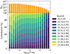 |
Fig. 4. Contribution of different redshift shells in Eq. (15) to the WD component of the AGWB for 25 frequency bins in the range [10−5, 1] Hz (bottom). The highest frequency bin does not contain any emission. The red lines indicate the total contribution of the z ≤ 0.5 Universe. The high redshift contributions are small for the simple model we use and overall the signal is dominated by the z ≤ 2 Universe. The number of double WD, summed over redshift, that source the AGWB for the different frequency bins (top). |
4. Discussion and conclusions
Given the amplitude of the WD component in Fig. 2, it is expected that it can be very well measured by LISA. Furthermore, the relative amplitudes show that, if LISA detects an AGWB signal in the mHz regime, it is likely dominated by the WDs. This means that it is likely hard to make statements about the BH (and NS) population based on a measurement of the AGWB unless there is a way to disentangle the two, or to detect the high-frequency component of the AGWB above 40 mHz.
In comparison to Farmer & Phinney (2003), the computation presented in this work results in a higher signal. They found ΩWD(1 mHz) = 3.57 × 10⁻¹², whereas we find ΩWD(1 mHz) = 5.7 × 10⁻¹². There are several factors that contribute to this difference. First, they use a star formation history that is about a factor of 2 lower than what we use, at least at the low redshifts that dominate the background. Secondly, their population synthesis code is different, which will lead to different results. As an indication, Farmer & Phinney (2003) find a local WD space density of 9 × 10⁻³ pc−3, whereas Nelemans et al. (2001b) – also using the SeBa code – find 19 × 10−3 pc−3. However, since 2001 the SeBa code has been significantly updated, so this comparison should not be taken as a specific value, but as an indication that a difference in normalisation of a factor ∼2 between codes is not surprising. Farmer & Phinney (2003) find a range of reference values between 1 × 10⁻¹² ≲ ΩWD(1 mHz)≲6 × 10⁻¹² in their models. Therefore, the value found in this work lies at the upper end of this range. We defer an in depth investigation of the variation of the shape and normalisation of the WD AGWB to future work.
Our estimate of the WD AGWB can be improved and extended in several ways, although this will not change our main conclusion that the WD AGWB likely dominates over the BH AGWB. First, we can do a study that takes the metallicity of the star formation (e.g., Chruslinska & Nelemans 2019) into account as done with SeBa before (e.g., van Oirschot et al. 2014; Korol et al. 2020), since metallicity can change the binary evolution. Additionally, there is also more and more evidence that metallicity also changes the initial binary parameters (Badenes et al. 2018; Moe et al. 2019). In addition, there are many uncertainties in binary evolution so a study varying these will give an indication of the astrophysical uncertainties in the model.
A more detailed model could also look into deviations from isotropy, since a significant fraction of the signal is found to originate in the nearby Universe, where the assumption of isotropy is not completely correct. This significantly complicates the modelling, but several studies showed that anisotropies could potentially be detected and contain information on the source population (e.g. Cusin et al. 2020). More detailed modelling will also offer more insight into the expected deviations of the signal from simple power laws and the shape of the turn over. This then provides input to detailed studies on the detectability of these features, for instance, with LISA. Finally, we note here that we neglected several types of binaries that will also contribute to the AGWB, albeit at a lower level than in the case of the double WD, such as interacting double WD binaries (AM CVn stars) and binaries containing helium stars or low-mass main sequence stars.
In conclusion, we simulated the WD AGWB using relatively little, but likely sufficient, detail to show that it will dominate over the AGWB from BH and NS binaries in the mHz regime. This offers an opportunity to study the WD binary population to much larger distances, while hampering the detection of the BH AGWB with missions such as LISA. The WD signal reaches a peak around 10 mHz and at higher frequencies the BH AGWB will become the dominant signal. The detectability of this transition by LISA and other mHz missions ought to be studied in detail.
Farmer & Phinney (2003) discretized the integral over cosmic time: dχ = −(1 + z) c dT. We have checked that our method is in agreement with the latter by calculating the AGWB using both discretizations. Furthermore, we have checked that increasing the number of redshift bins does not significantly alter the result.
Acknowledgments
We thank the referee for valuable suggestions and comments. G.N. is supported by the Dutch science foundation NWO. S.S. is supported by the Centre for Doctoral Training (CDT) at the University of Cambridge funded through STFC.
References
- Abadie, J., Abbott, B. P., Abbott, R., et al. 2010, Class. Quant. Grav., 27, 173001 [Google Scholar]
- Abbott, B. P., Abbott, R., Abbott, T. D., et al. 2016, ApJ, 818, L22 [Google Scholar]
- Abbott, R., et al. (LIGO Scientific Collaboration, Virgo Collaboration, & KAGRA Collaboration) 2021, Phys. Rev. D, 104, 022004 [NASA ADS] [CrossRef] [Google Scholar]
- Abbott, R., et al. (LIGO Scientific Collaboration, Virgo Collaboration, & KAGRA Collaboration) 2023a, Phys. Rev. X, 13, 041039 [Google Scholar]
- Abbott, R., et al. (LIGO Scientific Collaboration, Virgo Collaboration, & KAGRA Collaboration) 2023b, Phys. Rev. X, 13, 011048 [NASA ADS] [Google Scholar]
- Alonso, D., Contaldi, C. R., Cusin, G., Ferreira, P. G., & Renzini, A. I. 2020, Phys. Rev. D, 101, 124048 [NASA ADS] [CrossRef] [Google Scholar]
- Amaro-Seoane, P., Audley, H., Babak, S., et al. 2017, ArXiv e-prints [arXiv:1702.00786] [Google Scholar]
- Amaro-Seoane, P., Andrews, J., Arca Sedda, M., et al. 2023, Liv. Rev. Relat., 26, 2 [NASA ADS] [CrossRef] [Google Scholar]
- Auclair, P., Bacon, D., Baker, T., et al. 2023, Liv. Rev. Relat., 26, 5 [NASA ADS] [CrossRef] [Google Scholar]
- Babak, S., Caprini, C., Figueroa, D. G., et al. 2023, J. Cosmol. Astropart. Phys., 2023, 034 [CrossRef] [Google Scholar]
- Badenes, C., Mazzola, C., Thompson, T. A., et al. 2018, ApJ, 854, 147 [NASA ADS] [CrossRef] [Google Scholar]
- Baghi, Q. 2022, ArXiv e-prints [arXiv:2204.12142] [Google Scholar]
- Bavera, S. S., Franciolini, G., Cusin, G., et al. 2022, A&A, 660, A26 [NASA ADS] [CrossRef] [EDP Sciences] [Google Scholar]
- Binétruy, P., Bohé, A., Caprini, C., & Dufaux, J.-F. 2012, J. Cosmol. Astropart. Phys., 2012, 027 [CrossRef] [Google Scholar]
- Caprini, C., Durrer, R., & Servant, G. 2009, J. Cosmol. Astropart. Phys., 2009, 024 [CrossRef] [Google Scholar]
- Caprini, C., Hindmarsh, M., Huber, S., et al. 2016, J. Cosmol. Astropart. Phys., 2016, 001 [CrossRef] [Google Scholar]
- Christensen, N. 2019, Rep. Progr. Phys., 82, 016903 [CrossRef] [Google Scholar]
- Chruslinska, M., & Nelemans, G. 2019, MNRAS, 488, 5300 [NASA ADS] [Google Scholar]
- Cusin, G., Dvorkin, I., Pitrou, C., & Uzan, J.-P. 2020, MNRAS, 493, L1 [NASA ADS] [CrossRef] [Google Scholar]
- Dvorkin, I., Vangioni, E., Silk, J., Uzan, J.-P., & Olive, K. A. 2016, MNRAS, 461, 3877 [CrossRef] [Google Scholar]
- Edlund, J. A., Tinto, M., Królak, A., & Nelemans, G. 2005, Phys. Rev. D, 71, 122003 [NASA ADS] [CrossRef] [Google Scholar]
- Farmer, A. J., & Phinney, E. S. 2003, MNRAS, 346, 1197 [NASA ADS] [CrossRef] [Google Scholar]
- Hawking, S. W., & Israel, W. 1987, Three Hundred Years of Gravitation (Cambridge: Cambridge University Press) [Google Scholar]
- Karnesis, N., Babak, S., Pieroni, M., Cornish, N., & Littenberg, T. 2021, Phys. Rev. D, 104, 043019 [NASA ADS] [CrossRef] [Google Scholar]
- Keim, M. A., Korol, V., & Rossi, E. M. 2023, MNRAS, 521, 1088 [NASA ADS] [CrossRef] [Google Scholar]
- Korol, V., Toonen, S., Klein, A., et al. 2020, A&A, 638, A153 [NASA ADS] [CrossRef] [EDP Sciences] [Google Scholar]
- Kowalska-Leszczynska, I., Regimbau, T., Bulik, T., Dominik, M., & Belczynski, K. 2015, A&A, 574, A58 [NASA ADS] [CrossRef] [EDP Sciences] [Google Scholar]
- Kroupa, P. 2001, MNRAS, 322, 231 [NASA ADS] [CrossRef] [Google Scholar]
- Lehoucq, L., Dvorkin, I., Srinivasan, R., Pellouin, C., & Lamberts, A. 2023, MNRAS, 526, 4378 [NASA ADS] [CrossRef] [Google Scholar]
- Luo, J., Chen, L.-S., Duan, H.-Z., et al. 2016, Class. Quant. Grav., 33, 035010 [NASA ADS] [CrossRef] [Google Scholar]
- Luo, Z., Wang, Y., Wu, Y., Hu, W., & Jin, G. 2021, Progr. Theoret. Exp. Phys., 2021, 05A108 [CrossRef] [Google Scholar]
- Madau, P., & Dickinson, M. 2014, ARA&A, 52, 415 [Google Scholar]
- Moe, M., & Di Stefano, R. 2017, ApJS, 230, 15 [Google Scholar]
- Moe, M., Kratter, K. M., & Badenes, C. 2019, ApJ, 875, 61 [NASA ADS] [CrossRef] [Google Scholar]
- Nelemans, G., Yungelson, L. R., & Portegies Zwart, S. F. 2001a, A&A, 375, 890 [NASA ADS] [CrossRef] [EDP Sciences] [Google Scholar]
- Nelemans, G., Yungelson, L. R., Portegies Zwart, S. F., & Verbunt, F. 2001b, A&A, 365, 491 [NASA ADS] [CrossRef] [EDP Sciences] [Google Scholar]
- Nelemans, G., Yungelson, L. R., & Portegies Zwart, S. F. 2004, MNRAS, 349, 181 [NASA ADS] [CrossRef] [Google Scholar]
- Peters, P. C., & Mathews, J. 1963, Phys. Rev., 131, 435 [Google Scholar]
- Phinney, E. S. 2001, ArXiv e-prints [arXiv:astro-ph/0108028] [Google Scholar]
- Planck Collaboration VI. 2020, A&A, 641, A6 [NASA ADS] [CrossRef] [EDP Sciences] [Google Scholar]
- Portegies Zwart, S. F., & Verbunt, F. 1996, A&A, 309, 179 [NASA ADS] [Google Scholar]
- Punturo, M., Abernathy, M., Acernese, F., et al. 2010, Class. Quant. Grav., 27, 194002 [Google Scholar]
- Reitze, D., Adhikari, R. X., Ballmer, S., et al. 2019, Bull. Am. Astron. Soc., 51, 35 [Google Scholar]
- Renzini, A. I., Goncharov, B., Jenkins, A. C., & Meyers, P. M. 2022, Galaxies, 10, 34 [NASA ADS] [CrossRef] [Google Scholar]
- Schneider, R., Ferrari, V., Matarrese, S., & Portegies Zwart, S. F. 2001, MNRAS, 324, 797 [NASA ADS] [CrossRef] [Google Scholar]
- Schneider, R., Marassi, S., & Ferrari, V. 2010, Class. Quant. Grav., 27, 194007 [NASA ADS] [CrossRef] [Google Scholar]
- Thrane, E., & Romano, J. D. 2013, Phys. Rev. D, 88, 124032 [NASA ADS] [CrossRef] [Google Scholar]
- Toonen, S., Nelemans, G., & Portegies Zwart, S. 2012, A&A, 546, A70 [NASA ADS] [CrossRef] [EDP Sciences] [Google Scholar]
- van Oirschot, P., Nelemans, G., Toonen, S., et al. 2014, A&A, 569, A42 [NASA ADS] [CrossRef] [EDP Sciences] [Google Scholar]
All Tables
Order-of-magnitude estimates of the AGWB using the merger rate per Milky Way equivalent galaxy (MWEG) and a typical chirp mass of WD, BH, and NS binaries.
All Figures
|
Fig. 1. Density plot (linear scale) of the initial properties of the WD population: chirp mass, ℳ, versus GW frequency at the time of formation. |
| In the text | |
|
Fig. 2. Resulting WD component (thick salmon) of the AGWB compared to the LVK results (upper limit to BH/NS AGWB (dashed grey) and estimates for the BBH and BNS components in green and blue), the LISA Powerlaw Integrated sensitivity (black, Thrane & Romano 2013; Alonso et al. 2020), and an estimate of the Galactic foreground (brown) based on Karnesis et al. (2021). A fit to the WD component is shown in dark red. |
| In the text | |
|
Fig. 3. Comparison of the WD AGWB (salmon) and the broken power law fit (dark red) to a purely f2/3 signal (green dashed) by dividing the curves by f2/3. The WD AGWB deviates from the expected 2/3 slope, but the residuals (bottom) between the WD AGWB and the fit are below 5%. |
| In the text | |
|
Fig. 4. Contribution of different redshift shells in Eq. (15) to the WD component of the AGWB for 25 frequency bins in the range [10−5, 1] Hz (bottom). The highest frequency bin does not contain any emission. The red lines indicate the total contribution of the z ≤ 0.5 Universe. The high redshift contributions are small for the simple model we use and overall the signal is dominated by the z ≤ 2 Universe. The number of double WD, summed over redshift, that source the AGWB for the different frequency bins (top). |
| In the text | |
Current usage metrics show cumulative count of Article Views (full-text article views including HTML views, PDF and ePub downloads, according to the available data) and Abstracts Views on Vision4Press platform.
Data correspond to usage on the plateform after 2015. The current usage metrics is available 48-96 hours after online publication and is updated daily on week days.
Initial download of the metrics may take a while.