| Issue |
A&A
Volume 699, July 2025
|
|
|---|---|---|
| Article Number | A166 | |
| Number of page(s) | 14 | |
| Section | Planets, planetary systems, and small bodies | |
| DOI | https://doi.org/10.1051/0004-6361/202554168 | |
| Published online | 08 July 2025 | |
Grand theft moons
Formation of habitable moons around giant planets
1
Gothard Astrophysical Observatory, HUN-REN – ELTE Exoplanet Research Group,
Szent Imre herceg u. 112,
9700
Szombathely,
Hungary
2
HUN-REN Konkoly Observatory, Research Centre for Astronomy and Earth Science,
Konkoly-Thege Miklós út 15–17,
1121
Budapest,
Hungary
3
CSFK, MTA Centre of Excellence,
Budapest, Konkoly Thege Miklós út 15–17,
1121
Budapest,
Hungary
4
Kapteyn Astronomical Institute, University of Groningen,
9747
AD,
Landleven 12,
Groningen,
The Netherlands
★ Corresponding author: This email address is being protected from spambots. You need JavaScript enabled to view it.
Received:
18
February
2025
Accepted:
23
May
2025
Abstract
Context. Of the few thousand discovered exoplanets, a significant number orbit in the habitable zone of their star. Many of them are gas giants lacking a rocky surface and the solid water reservoirs necessary for life as we know it. The search for habitable environments can be extended to the moons of these giant planets. No confirmed exomoon discoveries have been made as of today, but promising candidates are known, and theories suggest that moon formation is a natural process in planetary systems.
Aims. We aim to study moon formation around giant planets in a phase similar to the final assembly of planet formation. We search for conditions for forming the largest moons with the highest possibility in circumplanetary disks, and we investigate whether the resulting moons can be habitable.
Methods. We determined the fraction of the circumplanetary disk’s mass converted into moons using numerical N-body simulations where moon embryos grow via embryo–satellitesimal collisions, which we investigated in disks around giant planets consisting of 100 fully interacting embryos and 1000 satellitesimals. In fiducial simulations, a 10 Jupiter-mass planet orbited a solar analog star at distances of 1–5 au. To determine the habitability of the synthetic moons, we calculated the stellar irradiation and tidal heating flux on these moons based on their orbital and physical parameters.
Results. We find the individual moon mass to be higher when the host planet orbits at a smaller stellar distance. However, moons leave the circumplanetary disk due to the stellar thief effect, which is stronger closer to the star. We find that 32% of synthetic moons can be habitable in the circumstellar habitable zone. Due to intense tidal heating, the incidence rate of moon habitability is similar at 2 au and decreases to 1% at larger distances (<5 au).
Conclusions. We conclude that the circumstellar habitable zone can be extended to moons around giant planets.
Key words: methods: numerical / celestial mechanics / planets and satellites: formation
© The Authors 2025
 Open Access article, published by EDP Sciences, under the terms of the Creative Commons Attribution License (https://creativecommons.org/licenses/by/4.0), which permits unrestricted use, distribution, and reproduction in any medium, provided the original work is properly cited.
This article is published in open access under the Subscribe to Open model. This email address is being protected from spambots. You need JavaScript enabled to view it. to support open access publication.
1 Introduction
The search for extraterrestrial life has traditionally meant hunting for exoplanets orbiting in the classical habitable zone of a solar analog star. However, the possibility of life should not be limited to this zone. An exomoon can also have the properties required for life as we know it (see, e.g., Williams et al. 1997; Kipping et al. 2009; Kaltenegger 2010). The most important properties for habitability are the solid silicate surface, which is the source of the building blocks of life, and the presence of liquid water on the surface, which acts as a solvent and a transfer medium for complex molecules (Lammer et al. 2009). Optimal atmospheric pressure and temperature are required for the presence of liquid water at the planetary surface, and the emergence and long-term evolution of life is conceivable in an environment similar to that on Earth. The probability of finding biomarkers could be increased by extending the search to Earth-sized exomoons orbiting giant planets in the circumstellar habitable zone (CSHZ). Moreover, the additional heat from tidal heating may make it possible to extend the region of liquid water beyond the outer edge of the CSHZ (Heller & Barnes 2013; Dobos & Turner 2015). The optimal mix of the heat from stellar irradiation, tidal heating, and other sources can provide a fertile environment for life (Heller 2012; Dobos et al. 2017).
The existence of the moons of giant planets in the Solar System as well as planet formation theories predict that the formation of regular moons is a common process (see, e.g., Peale & Canup 2015). As of today, a dozen promising exomoon candidates are known (e.g., Fox & Wiegert 2021; Oza et al. 2019), but none of them have been confirmed yet.
Regular moons assemble simultaneously with the formation of a planetary system in a circumplanetary (CP) disk. Of the many theories of moon formation, the following three appear to be the most widely accepted to describe the origin of the moons in the Solar System. 1) In the solid-enhanced minimum mass nebula model, a subnebula is detached from the protoplanetary disk by the growing giant planet. Moon formation starts with dust coagulation in the subnebula (Mosqueira & Estrada 2003). Moonlets on the order of 1000 km in size can be formed in 103– 104 years (Estrada et al. 2009). 2) In the gas-starve disk model, the protosatellite disk is fed by the infalling material from the circumstellar protoplanetary disk (Canup & Ward 2002; Ogihara & Ida 2012). The formation of Galilean moon-like satellites can last for 106 years in this theory (Heller & Pudritz 2015). 3) In the tidally spreading disk model, the moon formation process occurs as if moonlets were being made on an assembly line at the Roche limit of a giant planet, while the CP disk constantly spreads out-ward from inside of the Roche limit (Crida & Charnoz 2012). In this scenario, gas is already being dissipated from the disk, and the moonlets are being fed by the debris coming from the inside of the Roche limit (Fujii et al. 2017). Thus, the spreading disk describes a late formation theory.
The final assembly of regular moon formation could be characterized by collisions and pebble accretion. It can be assumed that the moons are assembled by processes similar to those of the rocky planets but scaled down to the size of satellite systems (Ronnet & Johansen 2020). During planet formation, planetesimals are formed from the dust component of the protoplanetary disk. In the final assembly phase, the gravitational interaction between planetesimals becomes the dominant force in the disk. Larger mass bodies accrete more mass, so they grow rapidly in the runaway growth phase (Greenberg et al. 1978). The perturbation of the largest mass neighbors produces an increasing velocity dispersion in the disk (Kokubo & Ida 1998). As a result, planetary embryos form in the oligarchic growth phase that are massive enough to perturb the orbits of less massive planetesimals (Ida & Makino 1993). Protoplanets form from the embryo − embryo and embryo − planetesimal collisions. After the gas has dissipated from the disk, planets form via protoplanet collisions in the post-oligarchic growth phase (Ronco et al. 2015). Based on the analogy of planet formation, in our study, we refer to planetesimals as satellitesimals and embryos as moon embryos (or simply embryos).
The formation of irregular moons (which do not form together with the planet) is usually explained by the following two theories. (1) CP disks can form after a giant impact event, and final assembly takes place in these disks as well, resulting in the formation of protosatellites (Canup & Asphaug 2001; Ronnet & Johansen 2020). (2) In addition, planets can acquire moons by capturing asteroids formed in the circumstellar disk (Debes & Sigurdsson 2007; Williams 2013).
In this study, we investigate the final phase of regular moon formation using numerical N-body simulations. Our model is primarily described by the final phase – and its continuation – of the solid-enhanced minimum mass nebula and the gas-starve CP disk scenarios. We calculated the gravitational interactions in CP disks consisting of fully interacting moon embryos embedded in a swarm of satellitesimals by applying a direct N-body integrator using GPUs. The semimajor axis of the planetary orbit and the mass of the host planet were varied. The gravitational field of the star can influence moon formation by stealing moons from the CP disk. Therefore, to study this effect, we compared two fiducial models: one that includes a central star and another that does not, for which case the external perturbing source acting on the CP disk is absent. We determined the parameters necessary to form the largest number and largest mass moons.
We investigated the habitability of moons assembled in the numerical simulations using a semi-analytical code. Taking into account the stellar irradiation, the stellar light reflected by the host planet, the thermal emission of the planet, and the heating from the planet − moon tidal interaction, we calculated the habitability of the synthetic moons based on the properties and the orbital elements of the moons from the results of the numerical simulations. Finally, we studied the habitability of moon candidates around exoplanets.
This paper is structured as follows. Section 2 is dedicated to the method of habitability calculations and the instance of possible habitable moons around known giant exoplanets. Section 3 presents a description of the numerical method applied for the N-body calculations. The results of the N-body simulations and habitability calculations are presented and discussed in Sect. 4. The main conclusions are summarized in Sect. 5.
2 Habitability of moons
2.1 Heat sources of satellites
The simplest CSHZ is a ring-shaped region around a star assuming an Earth-like planet. The extent of the ring depends on the stellar luminosity. Water can exist in liquid state on the surface of an Earth-mass (M⊕) planet orbiting between the boundaries of the CSHZ with an Earth-like atmosphere (e.g., Kasting et al. 1993). If the planet orbits closer to the central star than the inner edge of the CSHZ, the surface environment is too hot; if the planet orbits at a larger distance from the star than the outer edge of the CSHZ, the surface is too cold for liquid state water. However, habitable environments can be extended to the moons due to additional heat sources such as the stellar light reflected by the host planet, the thermal emission from the planet, and the heating from the planet − moon tidal interaction (Heller & Barnes 2013; Dobos et al. 2017). In addition to the stellar irradiation, the additional heat sources can provide a circumplanetary habitable zone (CPHZ) around the host planet for a given moon. It is important to note that the extent of the CPHZ depends strongly on the individual parameters of the moon.
For moons, the same incoming heat levels occur at different distances from the central star than it was predicted by Kopparapu et al. (2014) for planets, due to the presence of additional heat sources. The global energy flux on the moons can be significantly influenced by tidal heating, which comes from the tidal energy dissipation of the planet − moon interactions. The tidal heating rate in a viscoelastic satellite can be calculated using the following expression (e.g., Peale 2003; Meyer & Wisdom 2007):
![Mathematical equation: \[{H_{{\rm{tidal\;}}}} = \frac{{21}}{2}\frac{{{k_2}}}{Q}\frac{{GM_{{\rm{pl}}}^2{R^5}n{e^2}}}{{{a^6}}},\]](/articles/aa/full_html/2025/07/aa54168-25/aa54168-25-eq1.png) (1)
(1)
where G is the gravitational constant, Mpl is the planetary mass, R, n, e, and a are the radius, mean motion, eccentricity, and semimajor axis of the satellite, assuming a synchronous rotation. The mean motion can be written as n = (GMpl/a3)1/2. Q is the tidal dissipation factor and k2 is the second-order Love number of the satellite. The k2/Q parameter together describes the tidal response of the body and can be replaced by the imaginary number of k2, Im(k2) for a viscoelastic description of the rocky body (Segatz et al. 1988). Viscoelastic models are more realistic than models with a fixed k2/Q value because they include the temperature dependence of the viscosity (ηs) and the shear modulus (µs) of the rocky material. For calculating Im(k2), we follow the Maxwell model description of Henning et al. (2009), which was applied to exomoons for the first time by Dobos & Turner (2015). Based on Heller & Barnes (2013), we also calculated the stellar irradiation, the energy flux from the stellar light reflected by the planet and the thermal emission of the planet on the surface of a moon. We used a semi-analytical method to obtain the global heat flux on the moons. For more details on the habitability calculation, see Dobos et al. (2017).
2.2 A demonstration of moon habitability
To demonstrate that Earth-like habitable environments can also exist around giant planets, we collected a sample of giant exoplanets from the exoplanets.org database. We selected 461 known giant exoplanets with 1 MJ < Mpl < 13 MJ (MJ represents Jupiter-mass). We calculated the total incoming heat flux for the selected exoplanets, assuming tidal interactions with Earth analog putative moons in e = 0.05 orbit around their host planet. We did not specify the semimajor axes of the moon orbits. Instead, we examined the distance at which a moon must orbit the planet to receive the flux necessary for habitability. If no such distance can be defined where a putative moon can be habitable, then the planet does not have a CPHZ. When the orbit of the moon is inside the Roche limit or beyond the planetary Hill sphere, the moon also cannot be considered habitable due to the disintegration or orbital instability.
Figure 1 is an illustration of the phenomenon of how many giant exoplanets in our sample can have a putative habitable moon. The figure shows the luminosity of the exoplanets’ central stars as a function of the semimajor axis of the planetary orbits. The CSHZ boundaries are calculated using Eq. (4) of Kopparapu et al. (2014), where we assumed S eff⊙ values for 1 M⊕ moon. Conservative and optimistic habitable zone (HZ) limits are defined based on the climate models of Kopparapu et al. (2013), depending on the mass and the composition of the planetary atmospheres. The recent Venus limit refers to the inner boundary of the optimistic HZ. The runaway greenhouse limit defines the inner boundary of the conservative HZ. The environment for liquid water on the surface of an Earth-like planet orbiting in the conservative HZ is stable and optimal over long timescales. At the outer boundary of the conservative HZ, the heat from stellar irradiation drops to the level required for the maximum greenhouse limit. The outer boundary of the optimistic HZ is the early Mars limit, which assumes a relatively dense CO2 atmosphere, such as that supposed to have existed on Mars 3.8 billion years ago.
For moons, in addition to stellar irradiation, tidal heating can be a significant source of heat. The significance of tidal heating increases with the stellar distance. Figure 1 shows that based on the total incoming heat flux on the moons, the host planets are classified into the following categories: ∼ 74% of planets cannot host a habitable moon because the surface of the putative moon is too hot; however, about 26% of planets can have an Earth analog habitable moon. Among these, it is important to highlight the planets orbiting outside the CSHZ. The moons around these planets can be habitable due to the additional heat provided by tidal heating. This category accounts for almost half of the planets with a putative habitable moon in our sample. For a given stellar luminosity beyond a certain distance, even the additional heat from tidal heating is not sufficient to sustain habitability for a putative moon. We found three planets in this category.
We then estimated the region of CPHZ for a given planet at which an Earth analog moon in an e = 0.05 orbit can be habitable. Figure 2 illustrates an example of the CPHZ limits from a face-on view. In the case of HD 114386 b, we find that a putative moon orbit within a relatively broad range, between the recent Venus and early Mars limits, can be considered habitable. Since HD 114386 b orbits beyond the CSHZ of its K-type star, stellar irradiation gives only a relatively small contribution to the total heat flux on the moon. Instead, tidal heating becomes a crucial heat source, establishing a CPHZ where a putative moon can be habitable. Closer to the planet than the recent Venus limit, the moon would be too hot, while beyond the early Mars limit, it would be too cold for habitability.
Based on Eq. (1), one can see that the definition of the CPHZ is unique for each moon, and therefore, it is difficult to define generalized distance limits for the habitable zone around planets. However, one common feature can be derived for each exoplanet: as the planet orbits farther from the star, the limits associated with the heat flux levels necessary for habitability move closer to the host planet.
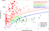 |
Fig. 1 Stellar luminosity as a function of the semimajor axis of 1 MJ < Mpl < 13 MJ exoplanet orbits derived from exoplanets.org. The limits of the circumstellar habitable zone (CSHZ) are displayed with colored curves: recent Venus (dashed red), runaway greenhouse (solid red), maximum greenhouse (solid blue), and early Mars (dashed blue) are based on Kopparapu et al. (2014). Planets are represented as colored dots whose size is proportional to |
![Mathematical equation: \[M_{{\rm{pl}}}^{1/3}\]](/articles/aa/full_html/2025/07/aa54168-25/aa54168-25-eq2.png)
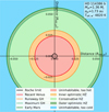 |
Fig. 2 Face-on view of the CPHZ of HD 114386 b assuming an Earth analog moon on e = 0.05 orbit around the planet. The axes represent the distance from the host planet in the planetary Hill radius. Roche (black), recent Venus (red), runaway greenhouse (orange), maximum greenhouse (light green), and early Mars (green) limits are displayed with solid circles. The shaded zones are the too hot region for habitability (red), inner optimistic habitable zone (orange), conservative habitable zone (light green), outer optimistic habitable zone (green), and too cold region for habitability (blue). |
3 N-body simulations of moon formation
We investigate the final phase of moon formation in CP disks with numerical N-body simulations. The final assembly of rocky bodies is calculated in CP protosatellite disks, which are gas-free in our model. The disks consist of moon embryos embedded in a swarm of satellitesimals, and the only force considered in the calculation is gravity. The central star, host planet, moon embryos, and satellitesimals are calculated as gravitationally fully interacting bodies.
The efficiency of planet formation can be used as an analogy to define the efficiency of moon formation. Moon formation efficiency can be defined as the ratio of the total mass of moons formed to the initial disk mass (Dencs & Regály 2021). We performed simulations to compare the formation efficiency in a stellar-centered (SC) and in a planet-centered (PC) scenario.
In the SC scenario, the central star is a solar analog. In order to model the formation of nearly Earth-mass moons, a 10 MJ giant planet is assumed to orbit the star in the fiducial model. Based on that the average density of the giant exoplanets of Fig. 1 is found to be ∼ 1.3 g cm−3, we assume a density of 1 ρJ and a radius of 2.61 RJ for the host planet. In the additional simulations, the mass of the giant planet is set to 2 and 5 MJ. The semimajor axis (apl) is set to 1, 2, 3, and 5 au in the different simulations. The initial eccentricity and inclination of the planetary orbit are both zero. In the PC scenario, we use the same initial conditions as in the SC scenario fiducial model, but the central star is removed, the 10 MJ planet is the new center of the system. In the PC simulations, there is no stellar perturbation in the system.
To determine the initial mass of the CP disk, we assume the formation of Earth-mass moons, which are important for the habitability investigations. The initial disk mass is set to 2 M⊕, for which case at least one Earth-mass moon may form due to the fact that the formation efficiency is less than 100%. Considering a 10 MJ planet, the disk-to-planet mass ratio is found to be of the order of 10−4 in agreement with the mass ratio generally assumed for regular moon systems by Canup & Ward (2006). In the additional simulations with 5 MJ and 2 MJ host planets, the masses of the protosatellite disks are reduced by 50 and 80%, respectively.
Assuming that a final assembly phase in a protosatellite disk is the scaled-down version of what occurs in a protoplanetary disk, we applied similar initial numbers and properties for embryos and satellitesimals as widely used in planet assembly N-body simulations (e.g., Kokubo & Ida 1998; Raymond et al. 2009; Ronco et al. 2015; Lykawka & Ito 2019; Clement & Chambers 2021). Initially, 100 embryos and 1000 satellitesimals were placed in the CP disk. We have previously shown that simulations containing fully interacting planetesimals in embryo − planetesimal disks are numerically convergent – meaning that the initial number of embryos does not affect the results – even with as few as 100 initial embryos (Dencs & Regály 2021).
The total embryo-to-satellitesimal mass ratio is 1:1. Thus, the individual masses of the embryos and the satellitesimals are 0.01 and 0.001 M⊕, respectively. The density of the embryos and satellitesimals is uniformly 3 g cm−3 (see, e.g., Lykawka & Ito 2019). Using a spherical approximation for the bodies, the radii of the embryos and the satellitesimals are set to 1.11 × 10⁻² Rpl (∼2037 km) and 5.18 × 10⁻³ Rpl (∼945 km), respectively.
The inner and the outer edges of the disk are determined based on the Roche and the Hill radii of the host planet, respectively. In this region, the orbits of embryos and satellitesimals can be stable on long timescales. Initially, we considered the orbit of Io as the inner boundary, scaled up for the case of a 10 MJ planet. Thus, the inner boundary is set at 5.16 RJ. We note that this is larger than the rigid Roche limit, and its use significantly reduces the runtime of the simulations. In the SC scenario, the host planet’s gravitational effect determines the orbit of the embryos and satellitesimals within the planetary Hill sphere. Beyond 0.49 × Hill radius, the embryos and satellitesimals are only weakly bound to the planet (Domingos et al. 2006). Therefore, we set a conservative 0.4 × Hill radius as the initial outer edge of the protosatellite disk. The Hill radius increases linearly with apl, and thus the distance of the outer edge of the disk from the host planet increases with the stellar distance. We used an increasing disk size for 1, 2, 3, and 5 au stellar distances. We note that the surface number density of the embryos and satellitesimals decreases with the increasing distance from the central star. In the PC scenario, we also used four different disk sizes referring to apl = 1, 2, 3, and 5 au cases in the SC scenario.
The angular positions and velocities of the embryos and satellitesimals are randomly distributed in the CP disk at the initial stage with the constraint that the initial surface number density of the disk is proportional to R−1 (Andrews & Williams 2007). In the fiducial model, we run ten simulations for each CP disk. The initial position and velocity of the embryos and satellitesimals are redistributed ten times for statistical studies. Figure A.1 shows the face-on view of the CP disks at the four different stellar distances. The initial and the final distributions of the embryos and satellitesimals are shown in the top and bottom panels, respectively.
All simulations are calculated in three dimensions. We study dynamically cold and hot disks in order to investigate the effect of the initial eccentricity and inclination distribution of embryos and satellitesimals on the formation of moons. In the case of larger mutual orbital inclinations, collisions occur less frequently. Thus the embryo growth may be slower, and the efficiency of the moon formation may be lower in hot disks than in cold disks. The initial inclination distribution of embryo and satellitesimal orbits follows Rayleigh distribution. In cold and hot disks the peaks of the inclination distributions are at 2 × 10⁻⁴ and 4 × 10⁻⁴, respectively. The initial eccentricity distribution of embryo and satellitesimal orbits also follows Rayleigh distribution. Based on the estimations of, for example, Ida & Makino (1992); Kokubo & Ida (2000), 2i ∼ e, the peaks of the eccentricity distributions are at 4 × 10⁻⁴ and 8 × 10⁻⁴ in cold and hot disks, respectively.
The synthetic bodies interact with each other gravitationally, which can lead to the following outcomes. (1) The collision of two bodies results in one body containing the mass of the original bodies: impulse and mass conservation due to the perfectly inelastic collision. Only embryo − embryo and embryo − satellitesimal collisions are allowed. A collision occurs when the distance between the two bodies is less than the sum of their radii. (2) An object is accreted by the planet within the physical radius of the planet, but the mass of the object is not added to the mass of the planet. (3) The scattered body is accreted by the star within the stellar radius. (4) The scattered body is removed (R > 1000 au).
For the investigation, we used a numerical integrator that we developed, HIPERION1, which is a GPU-based direct N-body integrator. The calculations were performed on NVidia Tesla K20, K40, and K80 GPUs. We applied a fourth order Hermite scheme in the simulations (Makino & Aarseth 1992). An adaptive shared time-step method was applied at each integration step using the generalized fourth order Aarseth scheme (Press & Spergel 1988; Makino & Aarseth 1992) with a given η parameter, which controls the precision of the integrator. In our study, η = 0.025 was found to be optimal. The total energy of the system should be conserved, and therefore, the precision of the integrator can be described by the relative energy error in each iteration. The calculations were performed using double precision arithmetics. The relative energy error was determined by the instantaneous total energy (Ei) and the total energy of the initial system (E0) as (Ei − E0)/E0 (Nitadori & Makino 2008). The relative energy error was found to be on the order of 10−10–10−8, with the optimal η value at the end of the simulations.
Some embryos started to grow via embryo embryo or embryo − satellitesimal collisions, some of them remained small in weight, and others were scattered out from the protosatellite disk. The embryos that survived the oligarchic growth phase are considered moons at the end of the simulations. We note that on a timescale orders of magnitude longer than the interval investigated, moons can occasionally collide with each other or be accreted by the planet or the star in the post-oligarchic growth phase; however, investigation of these occurrences is beyond the scope of this study.
We must account for the presence of two timescales in our simulations. (1) The first timescale is measured in the number of the planetary orbits (this timescale is not the same in the different simulations). (2) The second timescale is defined by the number of orbits of the bodies in the protosatellite disk (it can be unified in our fiducial model). The second timescale is more relevant in moon formation dynamics. Protoplanets form typically within a 106–107 year timescale, which covers runaway and oligarchic growth phases (e.g., Kokubo & Ida 2000). It is plausible to assume that moon formation is faster than planet formation because of the spatially down scaled CP disk. The moon formation process can be completed within 104 years (e.g., Cilibrasi et al. 2018), which means ∼ 106 orbits in a protosatellite disk. Therefore, in our simulations, we apply an order of magnitude larger timescale: the integrations are finished after 1.5 × 10⁷ orbits, counted at the inner edge of the protosatellite disk in the simulations with 10 MJ planet. The simulations are calculated for 7.68 × 10⁴, 2.71 × 10⁴, 1.48 × 10⁴, and 0.69 × 10⁴ planetary orbits at 1, 2, 3, and 5 au stellar distances, respectively. For Mpl = 2 MJ and 5 MJ, the simulations ran for a longer time because, in the case of a smaller planet mass, the inner edge of the disk is located closer to the planet, resulting in a shorter orbital period at the inner boundary of the disk. The total mass of the embryos converges to a constant level on the integration timescale.
In one specific case for each of the four orbital distances in the fiducial model, the simulations were extended for 3 × 10⁷ orbits at the inner edge (see the bottom row of Fig. A.1) to verify the long-term stability of the resulting moons. The results confirm that no significant changes occur in the protosatellite disks and that the resulting moons’ orbital elements can be considered stable over the investigated timescale.
4 Results and discussion
4.1 Moon formation in the circumplanetary disk
Panels A and B of Fig. 3 show the evolution of the total embryo mass in the Mpl = 10 MJ SC and PC simulations, respectively. In the SC scenario, the average total embryo masses first increase, and then decrease, so they have maxima have maxima at ∼ 1.58 M⊕. In the PC scenario, the average masses also increase initially, and then only a relatively small decline occurs. The maxima of the average masses are at a higher level in the PC than in the SC simulations, and the maximum mass values are spread over a wider range in the PC than in the SC scenario. In the PC scenario, the maximum of the total embryo mass is inversely proportional with the increasing disk size.
The total embryo mass depends slightly on the stellar distance in the SC simulations. The largest mass loss occurs in the simulations where the planet orbits at 1 au. Thus, the efficiency of moon formation is the lowest in these disks. The highest average efficiency is achieved at 2 au stellar distance in the SC simulations in cold disks. In the PC simulations, we find that the formation efficiency is inversely proportional to the disk size in both cold and hot disks. The total mass of the embryos is larger in the PC (1.66 M⊕ on average) than in the SC simulations (1.31 M⊕ on average) at the end of the simulations. Based on this, the total embryo mass of the SC simulations could reach a higher peak, but an effect outside the disk limits the maximum mass that embryos can accrete.
As an additional explanation for panels A and B, Fig. 4 shows how the time required to reach the peak mass depends on the size of the CP disk. One can see that as the distance of the outer edge of the disk from the host planet increases, so does the time taken to reach the peak in total embryo mass in both cold and hot disks. In general, the maxima are reached later in the PC than in the SC scenario. In the apl = 1 au SC simulations, the average total embryo mass reaches the peak after about 105 orbits at the inner edge of the disk. The peak is delayed in time with the distance from the central star: in apl = 2, 3, and 5 au simulations the total embryo mass peak is reached after 106, 2 × 10⁶, and 4 × 10⁶ orbits, respectively. In the apl = 1 au PC simulations, the total embryo mass reach its peak after 2 × 10⁶ orbits, and the time of the peak is also delayed with increasing disk size.
After the peak level is reached in the SC scenario, the total embryo mass starts to decrease due to the embryos being scattered out from the protosatellite disk. The observed phenomenon can be explained by the following train of thought. The close encounters of the embryos excite each other’s eccentricities. In smaller size disks, close encounters occur more frequently due to the higher surface density of the embryo distribution. The peak of the eccentricity distribution of the embryo orbits shifts to higher values than the initial eccentricity peak. The outermost excited embryos leave the protosatellite disk and begin to orbit the central star. Thus, in the case of SC simulations, the efficiency of moon formation is determined by two components: the surface number density of the bodies in the disk and the stealing effect of the central star.
The major trend in the embryo mass evolution is the same in the cold and hot disks. However, the standard deviation of the final total mass is larger in the hot disks than in the cold disks. The average efficiency of moon formation is quite similar in the cold and hot disks: the difference in the efficiency is only 2% in favor of the cold disks. This discrepancy can be explained by the fact that the average inclination is larger in the hot disks than in the cold disks. The mutual inclination of the bodies in the disks is relatively large in the hot disks. Thus, the probability of collisions is lower in the hot disks than in the cold disks.
Panel C of Fig. 3 displays the evolution of the total disk mass (moon embryos and satellitesimals) in SC simulations. The embryos accrete satellitesimals by collisions, which do not change the total mass of the disks. But after 7 × 10⁴ orbits, the disk starts to lose mass because some embryos and satellitesimals are removed from the disk. The total mass decay time is proportional to the distance of the planet from the star. On average, 40% and 30% of the initial disk mass are lost in apl = 1 au and 5 au simulations, respectively. The mass evolution of the dynamically cold and the hot disks are very similar. However, the average disk mass is lower in the hot disks than in the cold disks. Panel D of Fig. 3 shows the evolution of the disk mass in the PC scenario. In these cases, the disk mass is almost constant. Only a relatively small mass loss occurs, which can be explained mainly by the accretion of the host planet and a relatively small number of ejections from the system.
Panel E of Fig. 3 shows the evolution of the average eccentricity of the moon embryo orbits (⟨e⟩ embr) in the SC scenario. The evolution of ⟨e⟩ embr correlates with the evolution of the total embryo mass for each stellar distance. The peak of the average ⟨e⟩ embr of SC simulations is at 0.31. After reaching the peak, the average ⟨e⟩ embr begins to decrease as the embryos in high-eccentric orbits leave the protosatellite disk due to the stellar stealing or planetary accretion. The average ⟨e⟩ embr converges to the same level between 0.15 and 0.25. However, it has not converged by the end of the apl = 5 au simulations.
Panel F of Fig. 3 shows the evolution of the ⟨e⟩ embr in the PC scenario, where the ⟨e⟩ embr behaves the same way as in the SC scenario. This is because the high-eccentric embryos leave the disk, either by being accreted by the planet or by being ejected from the disk. However, the ⟨e⟩ embr values are higher in the PC than in the SC simulations. This is because the high-eccentric embryos do not leave the disk in such a large numbers in the PC than in the SC scenario due to the stellar stealing.
Panels G and H of Fig. 3 show the evolution of the number of embryos in the SC and PC scenarios, respectively. It can be seen that the number of embryos decreases over time. In the SC scenario, the number of embryos decreases for two reasons: collisions between embryos and their ejection from the disk. Since the probability of close encounters between embryos decreases with the increasing size of the disk, the number of embryos is always higher in the larger disks. One can see that in apl = 1, 2, and 3 au simulations, the number of embryos converges to a constant value between 1 and 25 for both cold and hot disks2. The number of the surviving embryos is higher in disks more distance from the star. We note that in the apl = 5 au simulations, the number of embryos has not yet fully saturated. In this case, the longevity of the simulation is not sufficient for the convergence.
For an embryo to be ejected from the disk, its eccentricity must be excited above a critical eccentricity value. In the SC scenario, the embryo eccentricity must be at least 0.6 and 0.9 to be accreted by the planet from the inner and from the outer edges of the disk, respectively. To escape outward from the disk (assuming an apocenter distance of, e.g., 150% of the disk’s outer edge), only e > 0.2 is needed for an embryo orbiting at the outer edge, while e > 0.5 is required from the inner edge. This shows that embryos closer to the inner edge are more easily accreted by the planet, while those near the outer edge are more likely to be stolen by the star. In the PC scenario, there is no perturbing star affecting the disk, and the gravitational field of the planet dominates throughout the entire integration. Thus, e > 0.6 is also required for accretion from the inner edge, but e ≥ 1 is required for ejection from the system. Therefore, it is harder to eject embryos from the disks in the PC scenario than in the SC scenario.
In the PC scenario, we find ejections from the disk less frequently than in the SC simulations. Therefore, the decrease in the number of embryos mainly occurs due to collisions in the PC scenario. By the end of the simulations, more embryos survive in the disks in the PC than in the SC scenario. The number of embryos converges to 5 − 40 in the PC simulations in both cold and hot disks. For the two largest initial disk sizes, the number of embryos is not yet fully saturated, as the timescale required for the perfect saturation is longer than the simulation time. Since the total embryo mass reached its maximum in all simulations, from that point on, any decay in the number of embryos can only result from embryos being ejected from the system.
The number of satellitesimals decreases for the same reason as the number of embryos. Since no collisions occur after 5 × 10⁶ orbits, the number of satellitesimals only decreases due to ejection from the disks. The final number of satellitesimals is less than 300 in both cold and hot SC simulations. The mass of each satellitesimal is assumed to be unchanged, and therefore their total mass is directly proportional to their number. The number of surviving satellitesimals increases with the distance from the star. 3 out of 10 apl = 1 au simulations show no surviving satel-litesimals, whereas in apl = 5 au, at least 180 survive in all 10 simulations. In the PC scenario, the number of satellitesimals converges to 60 − 450 in both cold and hot disks. We find that a significantly larger number of satellitesimals remain in the disks in the PC scenario than in the SC scenario. This can be explained by the same critical eccentricities required for ejection as for the embryos. As a general conclusion, the effect of the star can accelerate the drop of the number of embryos and satellitesimals in the SC scenario.
By the end of the SC simulations, the mass of the disk decreases by 30–40%, approximately 20% is accreted by the star and the planet, 10–20% is ejected from the system, and 1–5% remains outside the disk within the stellar-dominated field for a relatively long time. The total mass of bodies orbiting the star is proportional to the stellar distance of the former host planet, and the total mass of bodies ejected from the system is inversely proportional to that distance. By the end of the PC simulations, however, more than 90% of the initial disk mass remains in the disks, as there is no perturbing star to steal bodies from the disks. Moreover, a significant planetary accretion occurs, which is responsible for nearly a 10% reduction of the disk mass. The bodies ejected beyond the integration limit represent only a negligible amount of mass.
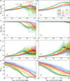 |
Fig. 3 Evolution of the moon embryos and the protosatellite disks of 10 MJ host planets on a logarithmic timescale. The left and right panels show the SC and the PC scenarios, respectively. Green, yellow, red, and blue colors indicate the apl = 1, 2, 3, and 5 au simulations, respectively. Shaded regions represent the range between the minimum and maximum values from the ten simulations of each initial condition. Dark and light shadings indicate the initially cold and hot disks, respectively. Solid and dotted lines show the average values of the cold and the hot disk simulations. Panels A and B show the total embryo mass, panels C and D show the total disk mass, panels E and F show the average orbital eccentricity, and panels G and H show the number of embryos in the disks. All simulations start from the same level. Arrows indicate the maxima of the average total embryo masses in the SC scenario. |
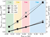 |
Fig. 4 Time for the average total embryo mass to reach its maximum as a function of the size of the disks. The time is displayed in terms of the number of orbits at the inner edge of the CP disk on the left vertical axis as well as in years on the right vertical axis. The disk size is expressed as the distance of the disk’s outer edge from the 10 MJ host planet. Black and gray curves display the cold and the hot disks, respectively. Solid and dotted lines show the SC and PC scenario, respectively. The shading of the background color indicates the same stellar distances as in Fig. 3. |
4.2 The resulting moons
The surviving embryos in the disks are considered to be moons. First, we investigate the cold disk simulations. Panel A of Fig. 5 shows the average number of moons in the disks as a function of disk size. It can be seen that the average number of moons increases with disk size (thus, with stellar distance in the SC scenario). In the Mpl = 10 MJ SC simulations, the average number of moons is 2.7 and 22.6 for 1 and 5 au stellar distances (from the average of 10 simulations), respectively. In the PC simulations, the average number of moons is 6.9 and 35 for the smallest and largest disks, respectively. This can be explained again by the stellar stealing effect in the SC cases. One can see that the average number of moons does not depend on the mass of the host planet for Mpl =2, 5 and 10 MJ SC simulations.
The average individual moon mass decreases with increasing disk size in each scenario, as shown in panel B of Fig. 5. The average individual masses are 0.46 M⊕ and 0.07 M⊕ at 1 and 5 au in Mpl = 10 MJ SC simulations, respectively. In the PC scenario, the average masses are 0.27 M⊕ and 0.04 M⊕ at 1 and 5 au, respectively. We find that the individual moon masses are ∼ 2.2 times larger in the SC than in the PC scenario. This can be explained by the stellar perturbation of the disks and the embryo theft in the SC cases. On average, approximately three times fewer surviving moons in the SC than in the PC simulations are found, while the total moon mass is ∼ 1.2 times larger in the PC scenario than in the SC scenario. We note that the average masses of the most massive moons are 0.74 M⊕ and 0.41 M⊕ in the 1 and 5 au SC simulations, respectively. Very similar to the SC values, 0.74 M⊕ and 0.43 M⊕ are found in the PC scenario.
One can see in panel B of Fig. 5 that the average individual moon mass increases with the mass of the host planet for each disk size. This phenomenon occurs due to the initial mass of the disks is scaled by the mass of the planet. Therefore, although the average number of moons is nearly the same in the SC simulations for disks of a given size, the average individual mass of the moons formed in lower-mass disks is smaller than in higher-mass disks.
Panel C of Fig. 5 shows the average eccentricity of the moons’ orbits as a function of disk size. In general, there is no clear correlation between the average eccentricity and disk size. The average eccentricities are higher in the PC simulations (⟨e⟩ moon = 0.31) than in the SC simulations (⟨e⟩ moon = 0.19) for Mpl = 10 MJ. This can be explained by the fact that highereccentric embryos can survive in the disk in the PC scenario. In the Mpl = 2 MJ and 5 MJ simulations, the average moon eccentricities are 0.14 and 0.15, respectively. This is because the fact that disks around lower-mass planets initially have lowermass embryos, which generate less eccentricity excitation in the disks3. We emphasize that the hot disk simulations give the same results as the cold ones within the standard deviation for the average number of moons, the average individual moon mass, and the average eccentricity of moons.
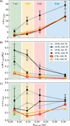 |
Fig. 5 Properties of the formed moons as a function of the size of the circumplanetary disks. Panel A shows the average number, panel B shows the average individual mass, and panel C shows the average eccentricity of the moons. Solid and dotted lines display the SC and the PC simulations, respectively. Black and gray lines are the simulations with cold and hot disks around Mpl = 10 MJ host planets. Vertical error bars indicate the standard deviation from the average values, which come from 10 simulations for each disk size. Red and orange lines display simulations with Mpl = 2 MJ and 5 MJ host planets, respectively. The colors of the shading indicate the same stellar distances as in Fig. 3. |
4.3 Habitability of the resulting moons
We calculated the habitability of the resulting moons by applying our semi-analytical method. We used the physical parameters and orbital elements of the resulting moons from the simulations to calculate the total heat flux reaching the surface of the moons. Based on the amount of incoming heat, we classified the moons into four categories: habitable, too hot for habitability, too cold for habitability, and too small to be habitable. A moon with a mass of M > 1 MMars is considered habitable if the total heat flux on the moon is between the recent Venus and the early Mars flux limits. A moon with a mass smaller than 1 MMars is not considered able to maintain a sufficiently large atmosphere for hundreds of millions of years, which is essential for the presence of liquid water on the surface. We note that Lammer et al. (2014) suggest 2.5 MMars for the minimum moon mass in the CSHZ of a solar analog star due to the strong stellar activity that can erode the atmosphere of a low-mass moon. At larger distances from the star (e.g., the distance of Mars), the impact of stellar activity on the atmosphere is weaker. Thus, even a lower-mass moon can retain a sufficiently massive atmosphere.
Table B.1 shows the number, the average mass, and the average eccentricity of the resulting moons of the fiducial model, separately for each habitability category. The average flux ratio of the tidal heating and stellar irradiation (⟨ Ftidal/Fstellar⟩) on the surface of the moons is also displayed. To provide a generic insight about the conditions that may result in habitable moons, the results of all moon formation simulations are shown together in each category. This helps in identifying some trends. Figure 6 shows the habitability of the moons as functions of the eccentricities and the semimajor axes from all simulations4. A horizontal dotted line displays the e = 0.1 eccentricity limit of moon orbits in each panel. Above this limit, we can estimate the global heat flux on the moons only with a relatively large uncertainty due to the characteristics of the viscoelastic model used for our calculations (see Dobos et al. 2017 for more details).
More than half of the resulting moons are too hot to be habitable around a planet orbiting at 1 au stellar distance, as can be seen in panels A and B of Fig. 6. Moons orbiting closer than 0.11 RHill,pl to the planet are too hot due to their proximity and relatively high eccentricity. Table B.1 shows that ⟨Ftidal/Fstellar⟩ ∼ 1 for too hot moons, which means that the tidal heating has the same significance as the stellar irradiation. However, we can find habitable moons between 0.12 and 0.33 × RHill,pl with relatively low eccentricities. At this distance from the planet, the effect of tidal heating is negligible. The average mass of the habitable moons is 0.52 M⊕ and 0.39 M⊕ in cold and hot disks, respectively.
Panels C and D of Fig. 6 show the apl=2 au simulations. There are no moons formed in the too hot category in the cold disk simulations. However, in the hot disks, we can find a few cases. In both cold and hot disks, more than half of the moons are too cold to be habitable. The average masses of habitable moons are found to be 0.48 M⊕ and 0.45 M⊕ in cold and in hot disks, respectively. Compared to the apl=1 au cases, the distance from the planet, where the habitable moons formed, is about 50% shorter for apl=2 au cases. Here, ⟨Ftidal/Fstellar⟩ ∼ 1.3 for both cold and hot disks, meaning that tidal heating has become the dominant heat factor for the habitability of the moons.
In the 3 au simulations, the most populated category is the moons with M < 1 MMars (see panels E and F of Fig. 6). A total of 7 and 5 habitable moons formed in the cold and in the hot disks, respectively, with average masses of 0.34 M⊕ and 0.3 M⊕. Here, the range in which habitable moons formed is very narrow. The significance of tidal heating is more than four times that of stellar irradiation concerning the habitability of moons. At 3 au stellar distance, there is only a small number of moons classified as too hot for habitability.
Panels G and H of Fig. 6 show the apl=5 au simulations. There are an order of magnitude more moons with M < 1 MMars mass at apl=5 au than at the other stellar distances. Larger mass moons are concentrated closer to the host planet. We find that most of these higher-mass moons are too cold to be habitable. Only a few habitable moons formed at a 5 au stellar distance. Here, tidal heating flux contributes to the heating of habitable moons about 10 times more than stellar irradiation. The possibility that a moon orbits within the narrow range where tidal heating is sufficient for habitability is very low. Therefore, we identify fewer habitable moons in this case. The average masses of the habitable moons are 0.3 M⊕ and 0.28 M⊕ in the cold and hot disks, respectively.
A general trend can be observed in the habitability of moons around 10 MJ planets: as the distance from the star increases, moons orbiting closer to the planet become habitable. This is because the stellar irradiation decreases with increasing distance from the star. The significance of tidal heating in the total heat flux on the habitable moons is proportional to the stellar distance. Another trend is that the number of M < 1 MMars moons is proportional to the stellar distance. This can be explained by the dynamics of moon formation. We also note that for 2 MJ and 5 MJ planets, the average individual moon mass is smaller on average than for a 10 MJ planet. Thus, the number of moons too small to be habitable is larger for smaller mass planets. Moreover, the average eccentricities are lower for a smaller planetary mass, reducing the effect of tidal heating.
As result of tidal evolution, the eccentricity of moons decreases in time. Based on the Constant Phase Lag model of Yoder & Peale (1981), the timescale of eccentricity decay is on the order of 1016 years for the habitable moons in Fig 6. We used the following equation for the estimation:
![Mathematical equation: \[{\tau _{\rm{e}}} = \frac{4}{{63}}\frac{M}{{{M_{{\rm{pl}}}}}}{\left( {\frac{a}{R}} \right)^5}\frac{{{\mu _s}Q}}{n},\]](/articles/aa/full_html/2025/07/aa54168-25/aa54168-25-eq3.png) (2)
(2)
assuming µs = 60 GPa and Q = 370 parameters, which are widely used values based on Earth’s average composition (see, e.g., Ji et al. 2010; Ferraz-Mello 2013).
We conclude that in the solar analog system, habitable moons are most commonly found in the apl = 1 and 2 au simulations, regardless of whether the moons formed in a cold or in a hot CP disk. At larger distances from the star, the tidal heating become the dominant heat source for the habitability of the moons. Due to tidal heating, habitable moons can form at larger stellar distances than the outer boundary of the classical CSHZ.
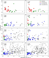 |
Fig. 6 Habitability of the moons formed in the disk of the 10 MJ planets. Each panel shows the eccentricity as a function of the semimajor axis of the moon orbits in units of the planet’s Hill radius. Left and right panels show the moons in dynamically cold and hot disks, respectively. Panels A and B show 1 au, panels C and D show 2 au, panels E and F show 3 au, and panels G and H show 5 au planetary orbit simulations. Habitable moons are indicated with green dots. Uninhabitable moons are classified into too hot (red dots), too cold (blue dots), and too small mass (black dots) categories. The size of the dots is proportional to the mass of the moons to the power of 1/3rd. In each panel, the horizontal dotted line shows the e = 0.1 upper eccentricity limit above that the confidence of the habitability calculations becomes less reliable. |
Known exoplanets that are similar to those in our model and can host a habitable assumed 1 M⊕ moon.
4.4 Habitability of exomoons in known systems
Using the 461 known exoplanets from the exoplanets.org database presented in Sect. 2.2, we selected the giant planets that most closely resemble the models calculated in our N-body simulations. We selected planets with mass 2 MJ < Mpl < 10 MJ, semimajor axis 1 au < Mpl < 5 au, eccentricity 0 < epl < 0.1, and host star luminosity 0.1 L⊙ < Lstar < 10.0 L⊙. We found that 9 of these planets can host a habitable moon which mass is assumed to be 1 M⊕. Table 1 shows the parameters of these planetary systems.
For planets orbiting beyond the outer edge of the CSHZ, tidal heating provides the habitability for the putative moon. We note that in systems with multiple planets, their gravitational interactions may destabilize the putative planet-moon system. We emphasize that our calculations assume a 1 M⊕ moon.
We also investigated the habitability of 12 exomoon candidates. Table 2 presents the candidates, the reason why they are not habitable, and the reference for the parameters. The eccentricity of the exomoon orbits is not available in most cases. Thus, we used an estimated eccentricity of e = 0.05 and a density of 3 g cm−3 for all exomoons. We find that the candidates are too hot to be habitable because they are too small (Io analogs) or orbiting too close to the host planet.
4.5 Caveats of the model and future investigations
Here, we address the important caveats of our model and possible directions for future studies. In our simulations, we applied perfectly inelastic collisions and neglected the effect of fragmentation. Chambers (2013) showed that the final mass of the protoplanets does not change significantly when fragmentation is neglected and the collisions are inelastic. This means a good approximation for the runaway growth phase. However, according to Haghighipour & Maindl (2022), fragmentation must be considered in the oligarchic growth model. Therefore, a future study is needed to investigate the effect of the inelastic collisions, as suggested by the model of Leinhardt & Stewart (2012).
We applied the simplification that the embryos and satel-litesimals have a uniform density, but the average density of the planetary or satellite seeds generally decreases with the increasing distance from the star due to the increasing mass fraction of ice in the composition (see, e.g., Ronnet et al. 2017). A more sophisticated model with distance-dependent densities should serve as the basis for a future study.
We note that the escape of moons from a circumplanetary disk might be important for the evolution of a planetary system. We found that even 1/3 M⊕ moons can move from the disk to circumstellar orbits. Sucerquia et al. (2019) call “ploonets” the circumstellar objects that originate from a protosatellite disk. The orbital evolution of ploonets can be influenced by the perturbations of the parent giant planet. Several papers have addressed this phenomenon (e.g., Namouni 2010; Yang et al. 2016), but investigation of the long-term evolution of ploonets is beyond the scope of our study.
Our investigation is limited to a solar analog star. For different stellar luminosities, the limits of the circumstellar as well as circumplanetary habitable zones would show a various picture. Moreover, the planetary Hill sphere decreases with the increasing stellar mass, making stellar stealing more effective.
The formation of irregular moons also not covered here. As we see by the Solar System moons, they are captured by giant planets that orbit at larger distances than 5 au from the Sun (see, e.g., Phoebe, Himalia). These moons orbit too far from their planet for tidal heating to be sufficient and are also too small-mass for habitability.
Habitability of the exomoon candidates.
5 Conclusions
In our study, we have investigated the efficiency of moon formation during the final assembly phase in the CPHZ. Our aim was to determine the conditions required for the habitability of moons. We used numerical N-body simulations with the GPU-based integrator HIPERION to compute the gravitational forces between star, planet, and circumplanetary bodies. In our fiducial simulations, fully interacting moon embryos and satellitesimals were placed in a disk around a 10 Jupiter-mass planet. The semi-major axis of the giant planet’s orbit was set to 1, 2, 3, and 5 au from a solar analog central star. The mass of the circumplanetary disk was set up based on the canonical 10−4 satellites-to-planet mass ratio. The size of the disks increases with stellar distance with a constant disk mass. To study the effect of the star on moon formation, we also performed simulations without a central star. We used dynamically cold and hot disks in terms of average eccentricities and inclinations. For statistical analysis, we ran ten simulations for each model, where the initial angular positions were distributed differently. In an additional setup, we ran single models for 2 and 5 Jupiter-mass planets. In the simulations, embryo − embryo and embryo − satellitesimal collisions (perfectly inelastic) were allowed, leading to the formation of moons. Using a semi-analytic code, we determined the habitability of the resulting moons after about 7 × 10⁴ years. We calculated the heat flux on the surface of the moons originating from stellar irradiation, tidal interactions between the planet and the given moon, reflected light from the planet, and thermal emission of the planet. We also applied our code to determine the habitability of 12 exomoon candidates.
In the moon formation simulations, we found that about 30 − 40% of the initial disk mass escapes from the circumplanetary disk due to the perturbations of the higher-mass embryos. Some of the embryos and satellitesimals can move beyond the outer edge of region of stable satellite orbits. Beyond the planetary Hill sphere, the embryos and satellitesimals are under the influence of the central star. Our main findings regarding the efficiency of moon formation can be summarized as follows:
The number of surviving moons and the growth rate of the moon embryos depend on the surface density (thus, the size) of the protosatellite disk during the collision regime. Larger surface densities result in larger mass moons and lower numbers of the surviving moons. The number of the resulting moons increases with the stellar distance; however, their individual mass decreases;
Stellar theft imposes an upper limit on the mass and the number of moons. In fact, the efficiency of the moon formation is significantly influenced by the central star;
Due to these two factors, the highest moon formation efficiency is observed for the planet orbiting at a 2 au stellar distance.
With regard to the habitability of the resulting moons, our main findings are the following:
Moons beyond 1 au can become habitable only because of tidal heating. At these stellar distances, the flux of tidal heating overcomes the stellar irradiation on the moons;
The number of habitable moons dramatically decreases with the distance from the star beyond 2 au. At 3 au and 5 au stellar distances, the CPHZ is extremely narrow. The optimal distance for habitability is between 1 − 2 au stellar distances;
Although the number of moons increases with the stellar distance, the mass of these moons is too small (lighter than 1 Mars-mass), and therefore they are not habitable.
We examined the habitability of putative Earth analog moons around 461 known giant exoplanets selected by their mass. We find that about a quarter of these planets could have habitable environments if the habitability region is extended to the CPHZ. Among these giant exoplanets, we found nine cases (Table 1) where the planet and its host star have similar properties to our model, and a 1 Earth-mass putative moon can be habitable around the planet. We also investigated the habitability of 12 exomoon candidates (Table 2). However, none of these exomoons was found to be habitable because they are too small or too hot. Our simulations show that moons with masses between Mars and Earth could form around planets with masses about ten times that of Jupiter, and many of these moons could potentially be habitable at 1 − 2 au stellar distances. These findings suggest that it is worth investigating not only rocky planets but also gas giants for Earth-like habitable environments. These locations provide suitable targets for the discovery of habitable exomoons or exomoons in general. Notably, space telescopes offer a new opportunity for this search. From 2025, the James Webb Space Telescope (Cycle 3) will observe exoplanetary systems with exomoon candidates based on the approved proposals, for example, Cassese et al. (2024); Pass et al. (2024). The PLATO mission could provide new results for exomoon research as well after its expected launch in 2026.
Acknowledgements
We thank the anonymous referee for useful suggestions that helped to improve the quality of the paper. This work was supported by the Hungarian Grant K119993. We acknowledge the Hungarian National Information Infrastructure Development Program (NIIF) for awarding us access to the computational resource based in Hungary at Debrecen. ZD acknowledges the support of the LP2021-9 Lendület grant of the Hungarian Academy of Sciences. ZD thanks to Gyula M. Szabó for the fruitful discussions.
Appendix A Demonstration of the change in the distributions of embryos and satellitesimals
To demonstrate the changes in the number and distribution of embryos and satellitesimals during the simulations, we provide Fig. A.1 that shows the face-on view of circumplanetary disks at four different stellar distances in the fiducial model. The top and bottom panels display the initial and final distributions of embryos and satellitesimals, respectively.
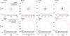 |
Fig. A.1 Distribution of the moon embryos (blue dots) and satellitesimals (gray dots) at the start (top panels) and the end (bottom panels) of the simulations in the face-on view of the protosatellite disks. Panels A, B, C, and D display the apl =1, 2, 3, and 5 au simulations. Orange dots correspond to the positions of the host planet. Brown and red circles indicate the initial inner and outer boundaries of the disks, respectively. Dashed red circle is the Domingos et al. (2006) suggested 0.4895 × Hill sphere’s outer edge. The time elapsed since the start of the simulations is shown at the bottom of each panel as a number of orbits at the inner edge of the circumplanetary disk, as well as, the orbit number of the host planet. |
Appendix B Habitability classification of the resulting moons
We provide Table B.1 to show the important properties of the resulting moons from the apl=1, 2, 3, and 5 au, Mpl = 10 MJ N-body simulations with dynamically cold and hot circumplanetary disks. Moons are divided into four categories based on the habitability calculations: too hot, habitable, too cold, and too small. The number, the average mass, and the average eccentricity of the moons are displayed in Table B.1. The flux ratio of the tidal heating and stellar irradiation on the surface of the moons is given for each category. The averaged results of all moon formation simulations of the fiducial model are shown in each category.
Classification of the resulting moons based on the habitability calculations.
References
- Andrews, S. M., & Williams, J. P. 2007, ApJ, 659, 705 [NASA ADS] [CrossRef] [Google Scholar]
- Boisse, I., Pepe, F., Perrier, C., et al. 2012, A&A, 545, A55 [NASA ADS] [CrossRef] [EDP Sciences] [Google Scholar]
- Canup, R. M., & Asphaug, E. 2001, Nature, 412, 708 [Google Scholar]
- Canup, R. M., & Ward, W. R. 2002, AJ, 124, 3404 [Google Scholar]
- Canup, R. M., & Ward, W. R. 2006, Nature, 441, 834 [NASA ADS] [CrossRef] [Google Scholar]
- Cassese, B., Batygin, K., Chachan, Y., et al. 2024, Revealing the Oblateness and Satellite System of an Extrasolar Jupiter Analog, JWST Proposal. Cycle 3, ID. #6491 [Google Scholar]
- Chambers, J. E. 2013, Icarus, 224, 43 [CrossRef] [Google Scholar]
- Cilibrasi, M., Szulágyi, J., Mayer, L., et al. 2018, MNRAS, 480, 4355 [NASA ADS] [Google Scholar]
- Clement, M. S., & Chambers, J. E. 2021, AJ, 162, 3 [NASA ADS] [CrossRef] [Google Scholar]
- Crida, A., & Charnoz, S. 2012, Science, 338, 1196 [Google Scholar]
- Debes, J. H., & Sigurdsson, S. 2007, ApJ, 668, L167 [Google Scholar]
- Dencs, Z., & Regály, Z. 2021, A&A, 645, A65 [NASA ADS] [CrossRef] [EDP Sciences] [Google Scholar]
- Dobos, V., & Turner, E. L. 2015, ApJ, 804, 41 [NASA ADS] [CrossRef] [Google Scholar]
- Dobos, V., Heller, R., & Turner, E. L. 2017, A&A, 601, A91 [NASA ADS] [CrossRef] [EDP Sciences] [Google Scholar]
- Domingos, R. C., Winter, O. C., & Yokoyama, T. 2006, MNRAS, 373, 1227 [NASA ADS] [CrossRef] [Google Scholar]
- Estrada, P. R., Mosqueira, I., Lissauer, J. J., D’Angelo, G., & Cruikshank, D. P. 2009, in Europa, eds. R. T. Pappalardo, W. B. McKinnon, & K. K. Khurana, 27 [Google Scholar]
- Ferraz-Mello, S. 2013, Celest. Mech. Dyn. Astron., 116, 109 [Google Scholar]
- Fox, C., & Wiegert, P. 2021, MNRAS, 501, 2378 [NASA ADS] [CrossRef] [Google Scholar]
- Fujii, Y. I., Kobayashi, H., Takahashi, S. Z., & Gressel, O. 2017, AJ, 153, 194 [Google Scholar]
- Gebek, A., & Oza, A. V. 2020, MNRAS, 497, 5271 [Google Scholar]
- Greenberg, R., Wacker, J. F., Hartmann, W. K., & Chapman, C. R. 1978, Icarus, 35, 1 [NASA ADS] [CrossRef] [Google Scholar]
- Gregory, P. C., & Fischer, D. A. 2010, MNRAS, 403, 731 [Google Scholar]
- Haghighipour, N., & Maindl, T. I. 2022, ApJ, 926, 197 [Google Scholar]
- Harakawa, H., Sato, B., Omiya, M., et al. 2015, ApJ, 806, 5 [Google Scholar]
- Heller, R. 2012, A&A, 545, L8 [NASA ADS] [CrossRef] [EDP Sciences] [Google Scholar]
- Heller, R., & Barnes, R. 2013, Astrobiology, 13, 18 [Google Scholar]
- Heller, R., & Pudritz, R. 2015, ApJ, 806, 181 [NASA ADS] [CrossRef] [Google Scholar]
- Henning, W. G., O’Connell, R. J., & Sasselov, D. D. 2009, ApJ, 707, 1000 [Google Scholar]
- Ida, S., & Makino, J. 1992, Icarus, 96, 107 [NASA ADS] [CrossRef] [Google Scholar]
- Ida, S., & Makino, J. 1993, Icarus, 106, 210 [NASA ADS] [CrossRef] [Google Scholar]
- Ji, S., Sun, S., Wang, Q., & Marcotte, D. 2010, J. Geophys. Res. (Solid Earth), 115, B06314 [Google Scholar]
- Kaltenegger, L. 2010, ApJ, 712, L125 [NASA ADS] [CrossRef] [Google Scholar]
- Kasting, J. F., Whitmire, D. P., & Reynolds, R. T. 1993, Icarus, 101, 108 [Google Scholar]
- Kipping, D. M., Fossey, S. J., & Campanella, G. 2009, MNRAS, 400, 398 [Google Scholar]
- Kokubo, E., & Ida, S. 1998, Icarus, 131, 171 [Google Scholar]
- Kokubo, E., & Ida, S. 2000, Icarus, 143, 15 [Google Scholar]
- Kopparapu, R. K., Ramirez, R., Kasting, J. F., et al. 2013, ApJ, 765, 131 [NASA ADS] [CrossRef] [Google Scholar]
- Kopparapu, R. K., Ramirez, R. M., SchottelKotte, J., et al. 2014, ApJ, 787, L29 [Google Scholar]
- Lammer, H., Bredehöft, J. H., Coustenis, A., et al. 2009, A&A Rev., 17, 181 [NASA ADS] [CrossRef] [Google Scholar]
- Lammer, H., Schiefer, S.-C., Juvan, I., et al. 2014, Origins Life Evol. Biosphere, 44, 239 [NASA ADS] [CrossRef] [Google Scholar]
- Leinhardt, Z. M., & Stewart, S. T. 2012, ApJ, 745, 79 [NASA ADS] [CrossRef] [Google Scholar]
- Lykawka, P. S., & Ito, T. 2019, ApJ, 883, 130 [Google Scholar]
- Makino, J., & Aarseth, S. J. 1992, PASJ, 44, 141 [NASA ADS] [Google Scholar]
- Meyer, J., & Wisdom, J. 2007, Icarus, 188, 535 [NASA ADS] [CrossRef] [Google Scholar]
- Minniti, D., Butler, R. P., López-Morales, M., et al. 2009, ApJ, 693, 1424 [NASA ADS] [CrossRef] [Google Scholar]
- Mosqueira, I., & Estrada, P. R. 2003, Icarus, 163, 198 [NASA ADS] [CrossRef] [Google Scholar]
- Naef, D., Mayor, M., Benz, W., et al. 2007, A&A, 470, 721 [NASA ADS] [CrossRef] [EDP Sciences] [Google Scholar]
- Naef, D., Mayor, M., Lo Curto, G., et al. 2010, A&A, 523, A15 [NASA ADS] [CrossRef] [EDP Sciences] [Google Scholar]
- Namouni, F. 2010, ApJ, 719, L145 [NASA ADS] [CrossRef] [Google Scholar]
- Nitadori, K., & Makino, J. 2008, New A, 13, 498 [NASA ADS] [CrossRef] [Google Scholar]
- Ogihara, M., & Ida, S. 2012, ApJ, 753, 60 [NASA ADS] [CrossRef] [Google Scholar]
- Oza, A. V., Johnson, R. E., Lellouch, E., et al. 2019, ApJ, 885, 168 [Google Scholar]
- Pass, E., Bean, J. L., Charbonneau, D., Cherubim, C., & Garcia-Mejia, J. 2024, A Search for Exoplanet Satellites that are the Same Size as the Earth’s Moon, JWST Proposal. Cycle 3, ID. #6193 [Google Scholar]
- Peale, S. J. 2003, Celest. Mech. Dyn. Astron., 87, 129 [CrossRef] [Google Scholar]
- Peale, S. J., & Canup, R. M. 2015, in Treatise on Geophysics, ed. G. Schubert, 559 [Google Scholar]
- Press, W. H., & Spergel, D. N. 1988, ApJ, 325, 715 [Google Scholar]
- Raymond, S. N., O’Brien, D. P., Morbidelli, A., & Kaib, N. A. 2009, Icarus, 203, 644 [NASA ADS] [CrossRef] [Google Scholar]
- Ronco, M. P., de Elía, G. C., & Guilera, O. M. 2015, A&A, 584, A47 [NASA ADS] [CrossRef] [EDP Sciences] [Google Scholar]
- Ronnet, T., & Johansen, A. 2020, A&A, 633, A93 [NASA ADS] [CrossRef] [EDP Sciences] [Google Scholar]
- Ronnet, T., Mousis, O., & Vernazza, P. 2017, ApJ, 845, 92 [NASA ADS] [CrossRef] [Google Scholar]
- Segatz, M., Spohn, T., Ross, M. N., & Schubert, G. 1988, Icarus, 75, 187 [NASA ADS] [CrossRef] [Google Scholar]
- Sucerquia, M., Alvarado-Montes, J. A., Zuluaga, J. I., Cuello, N., & Giuppone, C. 2019, MNRAS, 489, 2313 [NASA ADS] [CrossRef] [Google Scholar]
- Wang Sharon, X., Wright, J. T., Cochran, W., et al. 2012, ApJ, 761, 46 [NASA ADS] [CrossRef] [Google Scholar]
- Williams, D. M. 2013, Astrobiology, 13, 315 [Google Scholar]
- Williams, D. M., Kasting, J. F., & Wade, R. A. 1997, Nature, 385, 234 [NASA ADS] [CrossRef] [Google Scholar]
- Wittenmyer, R. A., Endl, M., Cochran, W. D., Levison, H. F., & Henry, G. W. 2009, ApJS, 182, 97 [Google Scholar]
- Wittenmyer, R. A., Horner, J., Tuomi, M., et al. 2012, ApJ, 753, 169 [CrossRef] [Google Scholar]
- Yang, M., Xie, J.-W., Zhou, J.-L., Liu, H.-G., & Zhang, H. 2016, ApJ, 833, 7 [Google Scholar]
- Yoder, C. F., & Peale, S. J. 1981, Icarus, 47, 1 [CrossRef] [Google Scholar]
We note that Fig. 3 shows the evolution on a logarithmic timescale to emphasize the maxima in total embryo mass. However, the saturation in the number of embryos is more apparent on a linear timescale. In most simulations, there is no accretion in the last 10% of the timescale, and ejections occur only at relatively long intervals.
Confirmed with supplementary simulations using the parameters of the fiducial model, but with lower-mass embryos and satellitesimals.
All Tables
Known exoplanets that are similar to those in our model and can host a habitable assumed 1 M⊕ moon.
All Figures
|
Fig. 1 Stellar luminosity as a function of the semimajor axis of 1 MJ < Mpl < 13 MJ exoplanet orbits derived from exoplanets.org. The limits of the circumstellar habitable zone (CSHZ) are displayed with colored curves: recent Venus (dashed red), runaway greenhouse (solid red), maximum greenhouse (solid blue), and early Mars (dashed blue) are based on Kopparapu et al. (2014). Planets are represented as colored dots whose size is proportional to |
| In the text | |
|
Fig. 2 Face-on view of the CPHZ of HD 114386 b assuming an Earth analog moon on e = 0.05 orbit around the planet. The axes represent the distance from the host planet in the planetary Hill radius. Roche (black), recent Venus (red), runaway greenhouse (orange), maximum greenhouse (light green), and early Mars (green) limits are displayed with solid circles. The shaded zones are the too hot region for habitability (red), inner optimistic habitable zone (orange), conservative habitable zone (light green), outer optimistic habitable zone (green), and too cold region for habitability (blue). |
| In the text | |
|
Fig. 3 Evolution of the moon embryos and the protosatellite disks of 10 MJ host planets on a logarithmic timescale. The left and right panels show the SC and the PC scenarios, respectively. Green, yellow, red, and blue colors indicate the apl = 1, 2, 3, and 5 au simulations, respectively. Shaded regions represent the range between the minimum and maximum values from the ten simulations of each initial condition. Dark and light shadings indicate the initially cold and hot disks, respectively. Solid and dotted lines show the average values of the cold and the hot disk simulations. Panels A and B show the total embryo mass, panels C and D show the total disk mass, panels E and F show the average orbital eccentricity, and panels G and H show the number of embryos in the disks. All simulations start from the same level. Arrows indicate the maxima of the average total embryo masses in the SC scenario. |
| In the text | |
|
Fig. 4 Time for the average total embryo mass to reach its maximum as a function of the size of the disks. The time is displayed in terms of the number of orbits at the inner edge of the CP disk on the left vertical axis as well as in years on the right vertical axis. The disk size is expressed as the distance of the disk’s outer edge from the 10 MJ host planet. Black and gray curves display the cold and the hot disks, respectively. Solid and dotted lines show the SC and PC scenario, respectively. The shading of the background color indicates the same stellar distances as in Fig. 3. |
| In the text | |
|
Fig. 5 Properties of the formed moons as a function of the size of the circumplanetary disks. Panel A shows the average number, panel B shows the average individual mass, and panel C shows the average eccentricity of the moons. Solid and dotted lines display the SC and the PC simulations, respectively. Black and gray lines are the simulations with cold and hot disks around Mpl = 10 MJ host planets. Vertical error bars indicate the standard deviation from the average values, which come from 10 simulations for each disk size. Red and orange lines display simulations with Mpl = 2 MJ and 5 MJ host planets, respectively. The colors of the shading indicate the same stellar distances as in Fig. 3. |
| In the text | |
|
Fig. 6 Habitability of the moons formed in the disk of the 10 MJ planets. Each panel shows the eccentricity as a function of the semimajor axis of the moon orbits in units of the planet’s Hill radius. Left and right panels show the moons in dynamically cold and hot disks, respectively. Panels A and B show 1 au, panels C and D show 2 au, panels E and F show 3 au, and panels G and H show 5 au planetary orbit simulations. Habitable moons are indicated with green dots. Uninhabitable moons are classified into too hot (red dots), too cold (blue dots), and too small mass (black dots) categories. The size of the dots is proportional to the mass of the moons to the power of 1/3rd. In each panel, the horizontal dotted line shows the e = 0.1 upper eccentricity limit above that the confidence of the habitability calculations becomes less reliable. |
| In the text | |
|
Fig. A.1 Distribution of the moon embryos (blue dots) and satellitesimals (gray dots) at the start (top panels) and the end (bottom panels) of the simulations in the face-on view of the protosatellite disks. Panels A, B, C, and D display the apl =1, 2, 3, and 5 au simulations. Orange dots correspond to the positions of the host planet. Brown and red circles indicate the initial inner and outer boundaries of the disks, respectively. Dashed red circle is the Domingos et al. (2006) suggested 0.4895 × Hill sphere’s outer edge. The time elapsed since the start of the simulations is shown at the bottom of each panel as a number of orbits at the inner edge of the circumplanetary disk, as well as, the orbit number of the host planet. |
| In the text | |
Current usage metrics show cumulative count of Article Views (full-text article views including HTML views, PDF and ePub downloads, according to the available data) and Abstracts Views on Vision4Press platform.
Data correspond to usage on the plateform after 2015. The current usage metrics is available 48-96 hours after online publication and is updated daily on week days.
Initial download of the metrics may take a while.