| Issue |
A&A
Volume 699, July 2025
|
|
|---|---|---|
| Article Number | A89 | |
| Number of page(s) | 29 | |
| Section | The Sun and the Heliosphere | |
| DOI | https://doi.org/10.1051/0004-6361/202553909 | |
| Published online | 02 July 2025 | |
Net radiative cooling rates and partial ionization in cool coronal condensations
1
Astronomical Institute, The Czech Academy of Sciences, 251 65 Ondřejov, Czech Republic
2
Center of Excellence ‘Solar and Stellar Activity’, University of Wroclaw, Wroclaw, Poland
3
Max-Planck-Institut für Astrophysik, Karl-Schwarzschild-Str. 1, 85740 Garching bei München, Germany
⋆ Corresponding author: This email address is being protected from spambots. You need JavaScript enabled to view it.
Received:
27
January
2025
Accepted:
18
May
2025
Abstract
Aims. We provide tabulated net radiative cooling rates (NRCRs) in the plasma of cool coronal condensations, together with the electron densities and ionization degrees describing its partial ionization. These readily applicable rates result from combined effects of the radiative cooling and radiative heating in the dominant atomic transitions in hydrogen, Mg II , and Ca II .
Methods. These NRCRs represent realistic estimates based on 1D non-LTE (i.e. departures from the local thermodynamic equilibrium) radiative transfer modelling that uses 1D isothermal and isobaric prominence models. To construct easy-to-use NRCR tables, we employed the concept of voxels (volume pixels), which allowed us to incorporate the essential information about the location of the modelled plasma with respect to the source of illumination. We provide tabulated values of NRCRs, electron densities, and ionization degrees for a broad range of plasma parameters representing a wide variety of cool coronal condensations, such as prominences, cool coronal loops, spicules, jets, and coronal rain.
Results. The accuracy of the provided voxel-based NRCRs, when tested against non-LTE calculations, is high, often showing a difference of only a few per cent. However, in some cases, the differences increase by up to a factor of two, which is the consequence of the assumptions and simplifications adopted here. Despite such differences, the voxel-based NRCRs that incorporate both the optically thick and thin radiative processes are a significant improvement, compared to the optically thin radiative loss formulas, when dealing with the cool plasmas at temperatures below 30 000 K.
Conclusions. The provided NRCRs are tabulated for three different scenarios of the orientation of the modelled structure with respect to the source of illumination: (i) a vertical orientation where a surface receives illumination from one half of the solar disc, (ii) a horizontal orientation where the bottom surface receives illumination from the entire solar disc, and (iii) a horizontal orientation where the top surface does not receive any illumination from the solar disc. This allows the voxel-based NRCRs to be implemented even in complex multi-dimensional simulations of cool coronal condensations.
Key words: radiation mechanisms: general / radiative transfer / Sun: corona / Sun: filaments, prominences
© The Authors 2025
 Open Access article, published by EDP Sciences, under the terms of the Creative Commons Attribution License (https://creativecommons.org/licenses/by/4.0), which permits unrestricted use, distribution, and reproduction in any medium, provided the original work is properly cited.
This article is published in open access under the Subscribe to Open model. This email address is being protected from spambots. You need JavaScript enabled to view it. to support open access publication.
1. Introduction
The aim of this paper is to provide tabulated net radiative cooling rates (NRCRs) in cool coronal condensations. These are structures such as prominences (e.g. Vial & Engvold 2015), cool coronal loops (e.g. Reale 2010), coronal rain (e.g. Antolin et al. 2015), spicules, and jets (e.g. Tsiropoula et al. 2012). They are composed of cool and dense plasma located within the hot and tenuous coronal environment. Another characteristic property of cool coronal condensations is the strong external illumination the plasma receives from the solar surface and the surrounding corona. This external source of radiation plays a significant role in the energy balance of the cool and dense plasma within the corona due to its high opacity in some atomic transitions. That leads to the absorption of the incident radiation and consequent radiative heating of the plasma. Such processes are coupled with the radiative cooling – the loss of energy due to escaping radiation in both the optically thin and thick atomic transitions. These complex radiative mechanisms are described in detail in, for example, Kuin & Poland (1991) and Heinzel et al. (2014).
A better understanding of NRCRs in the cool, externally illuminated plasma located in the solar corona can play an essential role in solving many open questions of modern solar physics. An example are the later stages of the formation of prominences, coronal rain, and coronal loops when their plasma cools to below about 30 000 K and becomes optically thick. The earlier stages of the formation of these structures were studied, for example, by Luna et al. (2012), Auchère et al. (2018), Antolin & Froment (2022), and Jerčić et al. (2024). Another example is the waves and oscillations in the prominence-like plasma, such as those studied by Ballester et al. (2016), Soler et al. (2021), Jerčić et al. (2022), and Liakh et al. (2023). Knowledge of NRCRs is also essential for highly realistic 3D simulations of prominences and their fine structures, such as those of Jenkins & Keppens (2022) and Donné & Keppens (2024). The radiative cooling and heating of the optically thick plasma of cool coronal condensations also play a role in their instabilities studied, for example, by Hillier (2018), Snow & Hillier (2024), and Antolin et al. (2022).
Here we provide readily applicable NRCRs resulting from the combined effects of the radiative cooling (radiation escaping the plasma volume) and radiative heating (due to absorption of the external illumination) in the dominant atomic transitions in hydrogen, Mg II, and Ca II. The tabulated NRCR values provided here represent a realistic estimate based on the non-LTE (i.e. departures from the local thermodynamic equilibrium) radiative transfer modelling in 1D prominence models. To provide practically usable tables of NRCRs for a wide variety of cool coronal condensations, we utilized the concept of voxels and tabulate the NRCRs for a wide range of plasma parameters. We also provide corresponding tables of electron densities and ionization degrees. The NRCR tables and the ionization degrees are provided in a simplified form in Appendices A, B, and C. The full versions of the tables, including the electron density values, are available at Zenodo1 (Gunár et al. 2025). The accuracy of the provided voxel-based NRCRs was tested against non-LTE calculations of NRCRs in 1D models that include temperature and pressure variations representing the prominence–corona transition region. These models were used, for example, by Anzer & Heinzel (1999). The correspondence between the non-LTE solutions and the estimates using the voxel-based tabulated NRCRs is very good, often with a difference of only a few per cent. However, in some parts of the modelled prominences, the differences can be up to a factor of two.
Nevertheless, despite such differences, the voxel-based tabulated NRCRs represent a significant improvement because no equivalent NRCR values, including optically thick radiation processes and external illumination in hydrogen, Mg II , and Ca II had been published before now. Kuin & Poland (1991) provided tables of optically thick NRCRs for hydrogen and helium. However, helium seems to be less important in cool plasmas while Mg II and Ca II are critically important coolants (Heinzel et al. 2014), as in the chromosphere (Vernazza et al. 1981). The optically thin radiation-loss formulas, such as those from Hildner (1974), Rosner et al. (1978), Milne et al. (1979), Schure et al. (2009), Soler et al. (2012), and others, have typically been used.
2. Models and their illumination
To derive NRCRs for a wide variety of cool coronal condensation use cases, we computed a large grid of 1D isothermal, isobaric, non-LTE models. These models solve the radiative-transfer problem in a 1D finite slab using the multi-level non-LTE code MALI1D (e.g. Heinzel 1995). We used the 5-level plus continuum atom model for hydrogen, Mg II and Ca II with the resonance lines treated with partial frequency redistribution. The same code was used also by Heinzel et al. (2014); see their Sect. 2 for further details. Helium is supposed to have a marginal effect on the electron density and also on NRCR and we did not include it in the models. The parameters of the models used to construct their large grid are described in Sect. 4.
Although the 1D models used here are isothermal and isobaric, the resulting NRCRs are not uniform. Due to the optically thick radiative transfer effects, NRCRs vary across the model width, as illustrated in Fig. 1. This NRCR variation within the models is the reason why we needed to adopt the concept of voxels (see Sect. 3). This concept allows us to describe the NRCRs with respect to the sources of the illumination. To derive such NRCRs, we used 1D non-LTE prominence models in two specific configurations – vertical 1D slab illuminated from both sides (Fig. 2, top) and horizontal 1D slab illuminated from below (Fig. 2, bottom). These two configurations allow us to take into account multiple scenarios of the illumination from the solar surface: i) illumination from the entire solar disc received by the bottom surface of the horizontal slab; ii) illumination from half of the solar disc received by the sides of the vertical slab; and iii) no illumination received by the top surface of the horizontal slab. Note that in the considered atomic transitions of hydrogen, Mg II and Ca II , the illumination from the surrounding corona is negligible.
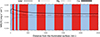 |
Fig. 1. Illustration of NRCRs as a function of the distance from the illuminated surface. Only one half (left) of the model width is shown (the model is symmetric). The plotted NRCR values correspond to a 1D vertical slab model with T = 6000 K and p = 0.5 dyn cm−2. The full line shows the total NRCRs derived as a sum of hydrogen (short-dashed black line), Mg II (dash-dotted black line), and Ca II (long-dashed white line) NRCRs. The blue and red stripes represent the voxels. The first five voxels have sizes of 50 km, and the rest have sizes of 250 km. |
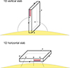 |
Fig. 2. Sketch of the configuration of the used models. Top: 1D vertical slab model symmetrically illuminated from both sides. Bottom: 1D horizontal slab model illuminated from below. The inlaid stripes visualize the geometry of the voxels in both orientations. |
On the other hand, the illumination from the solar surface in these transitions has a significant influence on the resulting NRCRs. Therefore, to provide tabulated NRCR values corresponding to a typical illumination of cool coronal condensations, we assume the modelled plasma to be static and at an altitude of 10 000 km. We adopted the incident radiation profiles emergent from the solar surface based on the observed values obtained during a minimum of solar activity. We used the Lyman-α reference profiles from Gunár et al. (2020), the reference profiles of the higher Lyman lines from Warren et al. (1998), and the reference Hα profiles from David (1961). The Mg II h &k reference profiles are from Gunár et al. (2021). The Ca II incident radiation profiles are a compilation of various observations made by Gorshkov, Heinzel, and Vial. These profiles were used, for example, by Gouttebroze et al. (1997) and Anzer & Heinzel (1999).
3. Voxels
To provide easy-to-use tables of NRCRs (together with electron densities and corresponding ionization degree), we use the concept of voxels – ‘volume pixels’ with defined sizes and known locations. These volume units allow us to divide the space occupied by the plasma in any model into blocks with nearly uniform plasma properties. For such blocks, tabulated values of NRCRs can be efficiently used and thus provide a good estimate of the balance of radiative processes in the entire modelled structures. In the 1D geometry that we are using here, voxels are equivalent to narrow 1D slices with the defined size (width) – see Fig. 2. In 2D geometry, voxels are equivalent to 2D columns and in 3D geometry to 3D blocks. For more details on the potential use of voxel-based NRCRs, see Sect. 9.
To maintain the balance between the granularity of the tabulated NRCRs and the usability of the provided tables, we adopted two specific sizes of voxels. In the proximity of the surfaces of the model, we used five narrow voxels with a size of 50 km. Starting at the distance of 250 km from the surface, we used voxels with sizes of 250 km. These voxel sizes allowed us to provide better precision within the near-surface layers where NRCRs are changing significantly – see the example in Fig. 1. In each voxel, we averaged the NRCR functions provided by models. This allowed us to derive representative NRCR values for each combination of temperature, pressure, and distance from the nearest surface. The distance from the nearest surface (L) specifies the location of each voxel with respect to the source of the illumination. L is one of the parameters describing the parametric space in which we tabulate the NRCRs (see Sect. 4). Note that L is defined as the distance from the nearest surface to the corresponding side of the voxel, not to its centre.
4. Parametric space
The grid of models used to calculate the NRCRs covers a wide range of temperatures, gas pressures and model widths – see Table 1. The temperature ranges from 6000 to 30 000 K, covering both the low-temperature cases and the temperatures at which the plasma becomes practically optically thin in most hydrogen, Mg II and Ca II atomic transitions (apart from the Lyman-α and Lyman-β lines; see e.g. Gunár et al. 2007). Note that at temperatures below 6000 K, the electron density can be enhanced by the ionization of metals. This idea was mentioned in Heinzel et al. (2024) but there are no quantitative estimates published up to date. We will consider this problem in the future.
Parameters covered by the grid of models.
The pressure ranges from low, coronal values of 0.03 dyn cm−2 up to the significant pressure of 1.0 dyn cm−2. The distance of voxels from the nearest surface L scales with the size of voxels we adopted (see Sect. 3). The L of the first voxel is equal to 0, followed by 50, 100, 150, 200, and 250 km. From that value, L increases in increments of 250 km. The width of the 1D slab models ranges from 500 to 10 000 km. However, to reduce the parametric space in which we tabulate the NRCRs, we used the mean values of NRCRs from models with identical T and p but varying widths. More details of the averaging over model widths are given in Sect. 5.
All models assume illumination corresponding to a static plasma at an altitude of 10 000 km above the solar surface. The incident radiation profiles correspond to the minimum of the solar activity. A choice of a different altitude, moving plasma, or other than solar minimum incident radiation will have an impact on the actual NRCR values. This is because the incident radiation is one of the most crucial input parameters for cool coronal condensations. It represents the dominant outer source of energy. Not only NRCRs but also the spectra emergent from externally illuminated cool-plasma structures in the corona change significantly with the illumination. Often, an increase (or decrease) in the intensity of the incident radiation can result in a comparative change in the spectra emergent from the observed structures. For example, Gunár et al. (2020, 2022) show that for Lyman lines and Mg II h &k lines, models with otherwise identical plasma parameters (temperature, pressure, etc.) will produce synthetic spectra modified by about 30% if the incident radiation is modified by the same amount. These findings may have considerable implications for the NRCR values, especially when we realize that the change in the incident radiation intensity between the minimum and maximum of the solar cycle can reach even up to 100% (see e.g. Gunár et al. 2020; Koza et al. 2022).
Complementary to the stage of the solar cycle, the altitude and the dynamics of the externally illuminated plasma also influence the incident radiation. The altitude modifies the incident radiation due to its dilution with the rising height above the solar surface and by the determination of the portion of the surface from which the illumination is received. For more details see Gunár & Heinzel (2024). Fast movement of the illuminated structures influences the incident radiation due to the Doppler shifts of the incident radiation profiles, causing the Doppler dimming/brightening effect (see e.g. Heinzel & Rompolt 1987; Vial & Engvold 2015; Peat et al. 2024).
To investigate the influence of different incident radiation (due to altitude, dynamics, or solar cycle), we need a systematic study that goes beyond the scope of the current paper. However, the NRCR values provided here for the altitude of 10 000 km, static plasma, and solar minimum illumination are realistic and correspond to typical illumination conditions in quiescent prominences. Moreover, the changes in temperature and pressure of the modelled plasma have a significantly larger influence on the NRCR values than the variations in the illumination.
5. Averaging across models with different widths
We used a grid of models in which, for each set of T and p, we have five models with different widths (D). This means that for each T and p combination, voxels with L = 0 to L = 200 km are present in five models (models with D of 500, 1000, 2000, 5000, and 10 000 km). Voxels with L = 250 km are present in four models (D of 1000, 2000, 5000, and 10 000 km). Voxels with L = 500 and L = 750 are in three models (2000, 5000, and 10 000 km), voxels with L = 1000 to L = 2250 km in two models (5000 and 10 000 km), and voxels with larger L in a single model.
While the influence of the model width on the actual NRCR values can be considerable (especially at higher temperatures) it is smaller compared to the influence of T or p within the dominant part of the parametric space. This allows us to take for each set of T, p, and L the mean value of NRCRs from all models in which the given voxel is present. That helps us reduce the parametric space and provide easy-to-use NRCR tables.
To demonstrate the dependence of NRCRs on the model width, we plot in Fig. 3 the total NRCRs from all models in the case of two selected voxels (L = 0 and L = 500 km). In both panels of Fig. 3, the x-axis gives the temperature while the pressure values are denoted by different symbols. The clusters of the same symbols represent the spread of NRCR values in models with different D but identical T and p. Note that the NRCR values are plotted for every combination of T, p, and D. Wherever the symbols appear not in clusters but as single data points, the spread of the NRCR values due to the model width is minimal. The clusters of the same symbols representing models with different D typically show a variation by about a factor of two. This is in most cases considerably smaller than the variations in NRCR values corresponding to models with differing T or p.
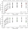 |
Fig. 3. Example of the total NRCRs in voxels with the distance from the nearest illuminated surface, L, of 0 and 500 km. The plots show all models from the grid. The temperature is given on the x-axis, and the pressure is indicated by the symbols. The asterisk (Λ) corresponds to 0.03 dyn cm−2, the diamond (♢) to 0.05 dyn cm−2, the square (□) to 0.1 dyn cm−2, the triangle (▵) to 0.3 dyn cm−2, the cross (×) to 0.5 dyn cm−2, and the plus sign (+) to 1.0 dyn cm−2. In each panel, we plot NRCR values from the 1D vertical slab models with all widths (500, 1000, 2000, 5000, and 10 000 km). The clusters of symbols (as indicated by the red and green ellipses) indicate the spread of the NRCR values from models with identical T and p but with different widths. Note that the voxel with L = 0 km is present in the models with all widths. The voxel with L = 500 km is present only in the models with widths of 2000, 5000, and 10 000 km. The seemingly missing data points in the grey zones are lower than the plotted range and are mostly negative. Negative NRCR values correspond to radiative gains. |
6. Tabulated NRCRs and ionization degrees
In the printed form in Appendices A, B, and C we provide quick-look tables of the total NRCRs – i.e. the sum of hydrogen, Mg II, and Ca II NRCRs. The tabulated total NRCRs are given for voxels with L between 0 and 1250 km. The NRCRs in voxels with larger L change only minimally with the increasing distance from the illuminated surface (see the example in Fig. 1). The full set of voxels is provided in the electronic tables described in Sect. 7. For each voxel, we tabulated the total NRCRs for all combinations of T and p covering the entire parametric space described in Sect. 4. The negative NRCR values (indicated in red) correspond to the radiative heating instead of cooling.
Tables A.1–A.5 correspond to 1D vertical models that receive illumination from a half of the solar surface (see Sect. 2 for more details). Tables B.1–B.5 correspond to the bottom surface of 1D horizontal models receiving illumination from the entire solar surface. Tables C.1–C.5 correspond to the top surface of 1D horizontal models that does not receive any illumination.
For each voxel, we provide corresponding plots of the total NRCRs. See Figs. A.1–A.3 for the 1D vertical models, Figs. B.1–B.3 for the bottom, and Figs. C.1–C.3 for the top surface of the 1D horizontal models.
Together with the total NRCRs, we provide the values of the ionization degree. The relationship between the ionization degree, electron density, and the local values of T and p can be described by the following formula:
 (1)
(1)
where N is the total particle number density given by N=nH+nHe+ne (we neglect other species). Here, nH is the total hydrogen density – the sum of the neutral hydrogen and the proton density, and nHe is the helium density. Assuming 10% abundance of the helium and no helium ionization for temperatures below 30 000 K, we can write
 (2)
(2)
where i is the hydrogen ionization degree defined as
 (3)
(3)
where we assume that ne=np. This assumption might not be correct at temperatures below 6000 K.
7. Electronic tables – NRCRs and electron density
On Zenodo2 (Gunár et al. 2025), we provide NRCR values separately for hydrogen, Mg II , and Ca II . The total NRCRs are then obtained as their sum. The NRCRs are tabulated for all voxels (L of 0, 50, 100, 150, 200, 250, 500, 750, etc. until 4750 km) and for each orientation of the model with respect to the source of illumination – the sides of the 1D vertical models, and the bottom and top sides of the 1D horizontal models.
Together with the NRCR tables, we also provide the electron densities for each combination of T, p, and L. The ionization degree can be derived from the provided electron densities using the following formula obtained from Eq. (2):
 (4)
(4)
8. Test of voxel-based NRCRs
To test the accuracy of the voxel-based NRCRs, we used 1D prominence models with varying temperature and pressure. These 1D vertical slab models, used in Anzer & Heinzel (1999), are based on the Kippenhahn & Schlüter magneto-hydrostatic equilibrium (Kippenhahn & Schlüter 1957), which determines the pressure variation. The temperature is prescribed semi-empirically and varies from 30 000 K at the boundary to Tmin at the centre of the slab. This variation corresponds to the lower prominence–corona transition region surrounding the cool prominence core.
Using two sets of input parameters as an example, we employed two different methods to derive NRCRs within the modelled prominence slabs. The first, more precise method relies on solving the non-LTE radiative transfer. The second method estimates the NRCRs within the modelled plasma using the voxel-based tabulated values provided here. To do so, we first determined to which voxel all grid points lying along the model width correspond to. Then, using the actual values of temperature and pressure at each grid point, we derived the NRCR values from the table corresponding to the given voxel by interpolating in T and p. In this way, we derived the estimated NRCRs along the width of each model. Figure 4 presents models M1_T8000 and M2_T8000, which differ in terms of the column mass parameter that determines the mass loading of the modelled prominence slab. That, via the Kippenhahn & Schlüter equilibrium, determines the pressure in the centre of the slab and also the width of the model (see Anzer & Heinzel 1999, for more details). Model M1_T8000 has a column mass of 1.8×10⁻⁴ g cm−2, resulting in a substantial central pressure of 0.735 dyn cm−2 and the total width of the slab of nearly 6000 km. M2_T8000 has a lower column mass of 6.7×10⁻⁶ g cm−2, producing significantly lower central pressure of 0.135 dyn cm−2 and a narrower total width of over 600 km. In both models, Tmin at the centre of the slab was set to 8000 K. Other parameters, such as the incident radiation or the height above the solar surface are identical as in the iso-thermal and iso-baric models used in the present work (see Sect. 4 for more details). Note that for this test, we computed nearly twenty models and selected two models in which the differences between the non-LTE solution and the voxel-based estimated NRCRs are the most pronounced.
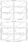 |
Fig. 4. Comparison of NRCRs derived by solving non-LTE radiative transfer and estimated, voxel-based NRCRs. The top six panels correspond to the model M1_T8000 and the bottom six panels to model M2_T8000. For both models, the first row of panels shows the variation in the temperature (left) and pressure (right) across one half of the symmetrical slab. The second row shows the total NRCRs (left) and hydrogen NRCRs (right). The third row shows the Mg II (left) and Ca II NRCRs (right). The voxel-based NRCR curves are plotted using dashed lines, while the non-LTE solution is plotted using the solid lines. |
When we compare the non-LTE solution and the voxel-based estimated NRCRs, we see a very good agreement between the two sets of NRCR curves along significant portions of the width of the models (Fig. 4). However, in several places, there are clear discrepancies. In some cases, the voxel-based NRCRs underestimate the true NRCR values, in other cases they overestimate them. These differences can in places reach up to a factor of two. Nevertheless, the estimated NRCR curves in general characterize the complex, double-peaked NRCR variations well.
In any case, some level of discrepancy between the non-LTE solution and the voxel-based estimate is to be expected. One reason is that the voxel-based tabulated NRCR values cannot provide the level of spatial resolution that is needed to fully describe fine-scale variations in complex models – see, for example, the sharp peak in the hydrogen NRCRs present within about 50 km of the surface of the second model shown in Fig. 4. Another reason is that to provide usable NRCR tables, we used the averaging across models with different widths (see Sect. 5 for more details). This averaging allows us to provide easy-to-use sets of voxel-based NRCRs that do not depend on the dimensions of the studied plasma structures. However, this simplification introduces potential inaccuracies, which might be as high as a factor of two – see Fig. 3 where the clusters of symbols indicate the spread of the NRCR values from models with identical temperature and gas pressure but with different widths. Such inaccuracies may account for the discrepancies of up to a factor of two that we see in the models used here as examples. In general, this level of inaccuracies is the consequence and the cost of the easy-to-use voxel-based concept of tabulated NRCRs constructed from isothermal, isobaric 1D models. For many numerically demanding applications, such a level of inaccuracy is a price worth paying. On the other hand, in cases when high-precision knowledge of the NRCRs is needed, the non-LTE solution will have to be adopted instead of voxel-based NRCR estimates.
9. How to use voxel-based tabulated NRCRs
The tabulated NRCRs provided here can be used in any geometry (1D, 2D, or 3D) if we know the temperature and pressure distributions of the modelled plasma. This is because any plasma structure can be divided into volume elements (voxels; see Sect. 3) in which the temperature and pressure can be assumed to be constant. Such isothermal and isobaric voxels can be as small as necessary. In the 1D geometry, the voxels will have the shape of narrow 1D slices, in 2D voxels are thin 2D columns, and in 3D they are 3D blocks. For each voxel, the tabulated NRCRs (given in erg s−1 cm−3) can be used to derive the radiative energy losses and gains. However, to do so accurately, the distance of each voxel from the nearest surface (L) needs to be identified. This is because the NRCRs in the externally illuminated plasma of cool coronal condensations vary with respect to the source of illumination. It means that in otherwise identical voxels (the same T, p, and L) the NRCR values are different if the voxel is near the bottom, side, or the top surface of a modelled structure. This difference is caused by the different amount of illumination each surface receives. For example, the bottom surface is illuminated from the entire solar surface visible to the modelled structure (see Gunár & Heinzel 2024 for more details). The top surface, on the other hand, does not receive any illumination from the solar surface.
The best way of dividing the modelled plasma into voxels and identifying their location with respect to the source of illumination will depend on the specifics of each use case. Likely, several implementation strategies may have to be tested to find the most efficient and accurate way of using the voxel-based NRCRs. We are open to provide assistance with the implementation upon being contacted. For illustration, we show here a simple scenario of a 2D horizontal model of a prominence (similar to e.g. Jejčič et al. 2014). The scheme of this scenario is shown in Fig. 5. In the figure, the enlarged view of the cross-section of the model is divided into voxels and colouring indicates the nearest respective surface to each voxel. In the case of yellow voxels, the nearest surface is at the bottom of the model, receiving the illumination from the entire (visible) solar surface. For the red voxels, the closest surface is at the sides of the structure, receiving the illumination from half of the solar surface. For the blue voxels, the nearest surface is at the top, where there is no illumination from the solar surface. The NRCR values for each voxel can be obtained from the provided tables specific to each case. Note that the voxels do not need to have a uniform size, which was adopted in Fig. 5 only for illustration purposes. In general, the dimensions of voxels will depend on the actual temperature and pressure distributions of the modelled plasma. The NRCR values corresponding to the actual T, p, and L of each voxel can be interpolated from the provided tables.
 |
Fig. 5. Sketch of a 2D horizontally infinite prominence model illuminated from the solar surface at its sides and the bottom. On the right is a close-up view of the model cross-section divided into voxels. For each voxel, the nearest surface of the model is indicated by a colour. For yellow voxels, the nearest surface is at the bottom of the model, receiving the illumination from the entire solar surface. For red voxels, the closest surface is at the sides, receiving the illumination from half of the solar surface. For the blue voxels, the nearest surface is at the top, where there is no illumination from the solar surface. |
10. Conclusions
In this paper we provide the first tabulated NRCRs for the plasma of cool coronal condensations that incorporate the optically thin and optically thick radiative transfer processes in the most important coolants – hydrogen, Mg II , and Ca II . This represents an extension of the work of Kuin & Poland (1991), who studied the atomic transitions in hydrogen and helium. The provided NRCR values are tabulated for a wide range of temperatures and gas pressures. The tables are easy to use thanks to the concept of voxels, which encapsulate essential information about the location of the plasma elements with respect to the source of illumination. In Appendices A, B, and C, we provide a simplified form of the NRCR tables, together with the intuitively understandable tables of the ionization degrees. The full form of the NRCR tables, together with the more general electron density values, are available on Zenodo3 (Gunár et al. 2025). These tabulated NRCRs can be used to study any cool coronal condensations and can be implemented even in complex, computationally demanding simulations. This makes the present paper a unique contribution to improved understanding of the energy balance in prominences, coronal rain, spicules, coronal loops, and other cool and dense plasma structures illuminated by radiation from the solar disc.
However, it is important to note that the provided NRCR values are only an estimate of the true NRCRs in the studied plasma. There are several assumptions and simplifications that we had to make to construct the easy-to-use voxel-based NRCR tables. Therefore, depending on the actual use cases, these assumptions will have a varying degree of influence on the accuracy of the NRCR estimates based on the tabulated NRCRs. It is thus essential to understand the assumptions used in this work and be aware of the impact they can be.
The first set of simplifications comes from the models we used to construct the NRCR tables. To encompass a large range of plasma parameters in a systematic way, we used 1D isothermal isobaric models. Such models are practical for constructing extensive grids. However, they become somewhat limiting when used to approximate significant variations in temperature and gas pressure within the modelled plasma. That is because the radiation field is not determined only by local thermodynamic conditions, but also by non-local conditions via the radiative transfer – hence the use of non-LTE radiative transfer modelling. The minor limitations of the NRCR tables constructed from isothermal isobaric models are already apparent in the examples shown in Sect. 8: we used models with varying temperature and pressure, resulting in differences between the voxel-based NRCRs and NRCRs derived from the non-LTE solution. These differences are typically rather small but can increase by up to a factor of two. This suggests that in cases where the temperature and pressure of the modelled plasma exhibit complex variations (such as in the 3D simulations of Jenkins & Keppens 2022 and Donné & Keppens 2024), even large differences can be expected.
The second important assumption we made in this work is the use of the illumination corresponding to a static plasma at an altitude of 10 000 km above the solar surface, with incident radiation profiles corresponding to the minimum of the solar activity. A choice of a different altitude, moving plasma, or a use of the incident radiation from other than the solar minimum part of the solar cycle will have an impact on the actual NRCR values (see e.g. Gunár et al. 2022; Gunár & Heinzel 2024; Peat et al. 2024). However, a systematic investigation of the true influence of different levels of incident radiation (due to altitude, dynamics, or the solar cycle) on the NRCRs is beyond the scope of the current paper. Moreover, the changes in temperature and pressure of the modelled plasma discussed below have a significantly greater influence on the NRCR values than the variations in the illumination.
The third simplification of the voxel-based NRCRs is the limited spatial resolution of the voxels. To provide usable NRCR tables, we could not tabulate NRCR values for a very large number of voxels. Rather, we used voxels of 50 km in size near the illuminated surfaces and 250 km in size deeper in the modelled structures (see Sect. 3 for more details). This choice, however, cannot provide the level of spatial resolution that is needed to fully describe any fine-scale variations encountered in complex models (such as those in Antolin et al. 2022, Jerčić et al. 2024, and Snow & Hillier 2024). Therefore, when studying significant small-scale changes in the temperature or gas pressure, some discrepancy between the true NRCRs and the NRCRs estimated from the voxel-based tables can be expected (see the discussion in Sect. 8).
Another important simplification is the averaging across the models with different widths described in Sect. 5. This allowed us to provide easy-to-use sets of voxel-based NRCR tables that do not depend on the dimensions of the studied plasma structures. However, this averaging also introduces potential inaccuracies as high as a factor of two.
While the influence of these simplifications on the accuracy of the provided NRCR tables may seem significant, it is in fact significantly less than the impact of the plasma properties that are encompassed in our NRCR tables. For example, from Figs. A.1–A.3, B.1–B.3, and C.1–C.3, it is clear that the variation in the gas pressure leads to the largest changes in the NRCR values, with differences exceeding three to four orders of magnitude. We can see this in the differences between the pressure at a given temperature. Variation in the temperature also causes large changes in the NRCRs, by up to two orders of magnitude. This can be seen when following the same pressure value along the temperature range. Most of this sensitivity is seen at low temperatures, between 6000 and 10 000 K.
The differences in the NRCRs between individual voxels, i.e. due to the distance from the nearest surface, are also significant. This is the especially case for the temperatures below 10 000 K. There, the differences between, for example, the voxels with L = 0 km and L = 1000 km can reach up to a factor of two to ten. However, even more importantly, the NRCR values can change from positive (signifying radiative cooling) to negative (signifying radiative heating). In such cases, the absolute magnitude of the change in NRCR values is not as critical as the different physical evolution of the studied structures. For example, when NRCRs become negative, any cooling of coronal condensations stops. This is an important distinction between the NRCRs from different voxels, but also a crucial distinction between the optically thick NRCRs provided here and the optically thin prescriptions discussed below.
The differences between NRCRs obtained from different orientations of the 1D model, and hence due to a changing amount of illumination, are similar in magnitude to the differences between voxels. Predictably, the largest variations, between factors of two and ten, are present in the voxels near the surface. This is especially true in the two extreme cases of full illumination at the bottom surface of the horizontal 1D slab (Appendix B) and the top surface of the horizontal slab, which does not receive any outside illumination from the solar disc (Appendix C). Consequently, the impact of the different levels of incident radiation (due to altitude, dynamics, or the solar cycle) can be expected to be considerably smaller than that from these two extreme cases.
The last issue we want to address is the distinction between the optically thick NRCRs provided here and the radiative cooling rates derived from optically thin radiative loss functions. A systematic study of the many available radiative loss functions (e.g. Hildner 1974; Rosner et al. 1978; Milne et al. 1979; Schure et al. 2009; Soler et al. 2012) is beyond the scope of this work. However, one clear advantage of the NRCRs provided here is the fact that the optically thick processes are, naturally, not encompassed in the optically thin radiative loss functions. They therefore cannot realistically describe situations in which cool coronal condensations reach a balance between radiative losses and gains, the radiative equilibrium (see Heinzel et al. 2014 for more details).
Data availability
The full form of the NRCR tables, together with the electron density values, are accessible at https://zenodo.org/records/15480951
Acknowledgments
S.G. and P.H. acknowledge the support from grant 25-18282S of the Czech Science Foundation (GAČR). S.G. and P.H. acknowledge the support from the project RVO:67985815 of the Astronomical Institute of the Czech Academy of Sciences.
References
- Antolin, P., & Froment, C. 2022, Front. Astron. Space Sci., 9, 820116 [NASA ADS] [CrossRef] [Google Scholar]
- Antolin, P., Vissers, G., Pereira, T. M. D., Rouppe van der Voort, L., & Scullion, E. 2015, ApJ, 806, 81 [Google Scholar]
- Antolin, P., Martínez-Sykora, J., & Şahin, S. 2022, ApJ, 926, L29 [NASA ADS] [CrossRef] [Google Scholar]
- Anzer, U., & Heinzel, P. 1999, A&A, 349, 974 [NASA ADS] [Google Scholar]
- Auchère, F., Froment, C., Soubrié, E., et al. 2018, ApJ, 853, 176 [Google Scholar]
- Ballester, J. L., Carbonell, M., Soler, R., & Terradas, J. 2016, A&A, 591, A109 [NASA ADS] [CrossRef] [EDP Sciences] [Google Scholar]
- David, K. -H. 1961, Z. Astrophys., 53, 37 [Google Scholar]
- Donné, D., & Keppens, R. 2024, ApJ, 971, 90 [CrossRef] [Google Scholar]
- Gouttebroze, P., Vial, J. -C., & Heinzel, P. 1997, Sol. Phys., 172, 125 [NASA ADS] [CrossRef] [Google Scholar]
- Gunár, S., & Heinzel, P. 2024, A&A, 687, A231 [NASA ADS] [CrossRef] [EDP Sciences] [Google Scholar]
- Gunár, S., Heinzel, P., Schmieder, B., Schwartz, P., & Anzer, U. 2007, A&A, 472, 929 [Google Scholar]
- Gunár, S., Schwartz, P., Koza, J., & Heinzel, P. 2020, A&A, 644, A109 [EDP Sciences] [Google Scholar]
- Gunár, S., Koza, J., Schwartz, P., Heinzel, P., & Liu, W. 2021, ApJS, 255, 16 [CrossRef] [Google Scholar]
- Gunár, S., Heinzel, P., Koza, J., & Schwartz, P. 2022, ApJ, 934, 133 [CrossRef] [Google Scholar]
- Gunár, S., Heinzel, P., & Anzer, U. 2025, https://doi.org/10.5281/zenodo.15480951 [Google Scholar]
- Heinzel, P. 1995, A&A, 299, 563 [NASA ADS] [Google Scholar]
- Heinzel, P., & Rompolt, B. 1987, Sol. Phys., 110, 171 [NASA ADS] [CrossRef] [Google Scholar]
- Heinzel, P., Vial, J. -C., & Anzer, U. 2014, A&A, 564, A132 [NASA ADS] [CrossRef] [EDP Sciences] [Google Scholar]
- Heinzel, P., Gunár, S., & Jejčič, S. 2024, Philos. Trans. R. Soc. Lond. Ser. A, 382, 20230221 [Google Scholar]
- Hildner, E. 1974, Sol. Phys., 35, 123 [Google Scholar]
- Hillier, A. 2018, Rev. Mod. Plasma Phys., 2, 1 [Google Scholar]
- Jejčič, S., Heinzel, P., Zapiór, M., et al. 2014, Sol. Phys., 289, 2487 [CrossRef] [Google Scholar]
- Jenkins, J. M., & Keppens, R. 2022, Nat. Astron., 6, 942 [NASA ADS] [CrossRef] [Google Scholar]
- Jerčić, V., Keppens, R., & Zhou, Y. 2022, A&A, 658, A58 [NASA ADS] [CrossRef] [EDP Sciences] [Google Scholar]
- Jerčić, V., Jenkins, J. M., & Keppens, R. 2024, A&A, 688, A145 [NASA ADS] [CrossRef] [EDP Sciences] [Google Scholar]
- Kippenhahn, R., & Schlüter, A. 1957, Z. Astrophys., 43, 36 [Google Scholar]
- Koza, J., Gunár, S., Schwartz, P., Heinzel, P., & Liu, W. 2022, ApJS, 261, 17 [NASA ADS] [CrossRef] [Google Scholar]
- Kuin, N. P. M., & Poland, A. I. 1991, ApJ, 370, 763 [Google Scholar]
- Liakh, V., Luna, M., & Khomenko, E. 2023, A&A, 673, A154 [NASA ADS] [CrossRef] [EDP Sciences] [Google Scholar]
- Luna, M., Karpen, J. T., & DeVore, C. R. 2012, ApJ, 746, 30 [Google Scholar]
- Milne, A. M., Priest, E. R., & Roberts, B. 1979, ApJ, 232, 304 [Google Scholar]
- Peat, A. W., Osborne, C. M. J., & Heinzel, P. 2024, MNRAS, 533, L19 [NASA ADS] [CrossRef] [Google Scholar]
- Reale, F. 2010, Liv. Rev. Sol. Phys., 7, 5 [Google Scholar]
- Rosner, R., Tucker, W. H., & Vaiana, G. S. 1978, ApJ, 220, 643 [Google Scholar]
- Schure, K. M., Kosenko, D., Kaastra, J. S., Keppens, R., & Vink, J. 2009, A&A, 508, 751 [NASA ADS] [CrossRef] [EDP Sciences] [Google Scholar]
- Snow, B., & Hillier, A. S. 2024, Philos. Trans. R. Soc. Lond. Ser. A, 382, 20230227 [Google Scholar]
- Soler, R., Ballester, J. L., & Parenti, S. 2012, A&A, 540, A7 [NASA ADS] [CrossRef] [EDP Sciences] [Google Scholar]
- Soler, R., Terradas, J., Oliver, R., & Ballester, J. L. 2021, ApJ, 909, 190 [Google Scholar]
- Tsiropoula, G., Tziotziou, K., Kontogiannis, I., et al. 2012, Space Sci. Rev., 169, 181 [Google Scholar]
- Vernazza, J. E., Avrett, E. H., & Loeser, R. 1981, ApJS, 45, 635 [Google Scholar]
- Vial, J. -C., & Engvold, O. 2015, Solar Prominences Astrophys. Space Sci. Lib., 415 [Google Scholar]
- Warren, H. P., Mariska, J. T., & Wilhelm, K. 1998, ApJS, 119, 105 [Google Scholar]
Appendix A: 1D vertical model
Appendix A provides tables of total NRCR values and ionization degree (Tables A.1 - A.5) for the 1D vertical models (see Fig. 2, top). These models receive the illumination from half of the solar surface on each side.
Total NRCRs (erg s−1 cm−3) and ionization degrees for voxels with L of 0 and 50 km – a side of 1D vertical models.
Total NRCRs (erg s−1 cm−3) and ionization degrees for voxels with L of 100 and 150 km – a side of 1D vertical models.
Total NRCRs (erg s−1 cm−3) and ionization degrees for voxels with L of 200 and 250 km – a side of 1D vertical models.
Total NRCRs (erg s−1 cm−3) and ionization degrees for voxels with L of 500 and 750 km – a side of 1D vertical models.
Total NRCRs (erg s−1 cm−3) and ionization degrees for voxels with L of 1000 and 1250 km – a side of 1D vertical models.
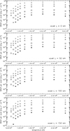 |
Fig. A.1. Total NRCRs in voxels with L of 0, 50, 100, and 150 km for the 1D vertical models (Tables A.1 and A.2). The temperature is given on the x-axis and the pressure is indicated by the symbols. Asterisks correspond to 0.03 dyn cm−2, diamonds to 0.05 dyn cm−2, squares to 0.1 dyn cm−2, triangles to 0.3 dyn cm−2, crosses to 0.5 dyn cm−2, and plus signs to 1.0 dyn cm−2. The seemingly missing data points in the grey zones are lower than the plotted range and are mostly negative. Negative NRCR values correspond to radiative gains. |
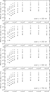 |
Fig. A.2. Same as Fig. A.1 but for voxels with L of 200, 250, 500, and 750 km for the 1D vertical models (Tables A.3 and A.4). |
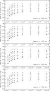 |
Fig. A.3. Same as Fig. A.1 but for voxels with L of 1000, 1250, 1500, and 1750 km for the 1D vertical models (Tables A.5). |
Appendix B: 1D horizontal model - Bottom surface
Appendix B provides tables of total NRCR values and ionization degree (Tables B.1 - B.5) for the bottom part of the 1D horizontal models (see Fig. 2, bottom). This surface receives the illumination from the entire solar surface.
Total NRCRs (erg s−1 cm−3) and ionization degrees for voxels with L of 0 and 50 km – bottom part of 1D horizontal models.
Total NRCRs (erg s−1 cm−3) and ionization degrees for voxels with L of 100 and 150 km – bottom part of 1D horizontal models.
Total NRCRs (erg s−1 cm−3) and ionization degrees for voxels with L of 200 and 250 km – bottom part of 1D horizontal models.
Total NRCRs (erg s−1 cm−3) and ionization degrees for voxels with L of 500 and 750 km – bottom part of 1D horizontal models.
Total NRCRs (erg s−1 cm−3) and ionization degrees for voxels with L of 1000 and 1250 km – bottom part of 1D horizontal models.
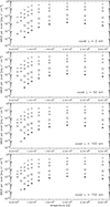 |
Fig. B.1. Total NRCRs in voxels with L of 0, 50, 100, and 150 km for the bottom part of 1D horizontal models (Tables B.1 and B.2). The temperature is given on the x-axis and the pressure is indicated by the symbols. Asterisks corresponds to 0.03 dyn cm−2, diamonds to 0.05 dyn cm−2, squares to 0.1 dyn cm−2, triangles to 0.3 dyn cm−2, crosses to 0.5 dyn cm−2, and plus signs to 1.0 dyn cm−2. The seemingly missing data points in the grey zones are lower than the plotted range and are mostly negative. Negative NRCR values correspond to radiative gains. |
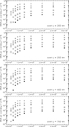 |
Fig. B.2. Same as Fig. B.1 but for voxels with L of 200, 250, 500, and 750 km for the 1D vertical models (Tables B.3 and B.4). |
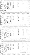 |
Fig. B.3. Same as Fig. B.1 but for voxels with L of 1000, 1250, 1500, and 1750 km for the 1D vertical models (Tables B.5). |
Appendix C: 1D horizontal model - Top surface
Appendix C provides tables of total NRCR values and ionization degree (Tables C.1 - C.5) for the top part of the 1D horizontal models (see Fig. 2, bottom). This surface does not receive any illumination.
Total NRCRs (erg s−1 cm−3) and ionization degrees for voxels with L of 0 and 50 km – top part of 1D horizontal models.
Total NRCRs (erg s−1 cm−3) and ionization degrees for voxels with L of 100 and 150 km – top part of 1D horizontal models.
Total NRCRs (erg s−1 cm−3) and ionization degrees for voxels with L of 200 and 250 km – top part of 1D horizontal models.
Total NRCRs (erg s−1 cm−3) and ionization degrees for voxels with L of 500 and 750 km – top part of 1D horizontal models.
Total NRCRs (erg s−1 cm−3) and ionization degrees for voxels with L of 1000 and 1250 km – top part of 1D horizontal models.
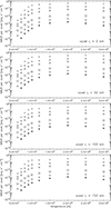 |
Fig. C.1. Total NRCRs in voxels with L of 0, 50, 100, and 150 km for the top part of 1D horizontal models (Tables C.1 and C.2). The temperature is given on the x-axis and the pressure is indicated by the symbols. Asterisks corresponds to 0.03 dyn cm−2, diamonds to 0.05 dyn cm−2, squares to 0.1 dyn cm−2, triangles to 0.3 dyn cm−2, crosses to 0.5 dyn cm−2, and plus signs to 1.0 dyn cm−2. The seemingly missing data points in the grey zones are lower than the plotted range and are mostly negative. Negative NRCR values correspond to radiative gains. |
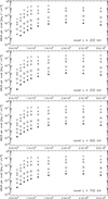 |
Fig. C.2. Same as Fig. C.1 but for voxels with L of 200, 250, 500, and 750 km for the 1D vertical models (Tables C.3 and C.4). |
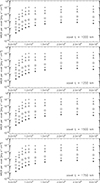 |
Fig. C.3. Same as Fig. C.1 but for voxels with L of 1000, 1250, 1500, and 1750 km for the 1D vertical models (Tables C.5). |
All Tables
Total NRCRs (erg s−1 cm−3) and ionization degrees for voxels with L of 0 and 50 km – a side of 1D vertical models.
Total NRCRs (erg s−1 cm−3) and ionization degrees for voxels with L of 100 and 150 km – a side of 1D vertical models.
Total NRCRs (erg s−1 cm−3) and ionization degrees for voxels with L of 200 and 250 km – a side of 1D vertical models.
Total NRCRs (erg s−1 cm−3) and ionization degrees for voxels with L of 500 and 750 km – a side of 1D vertical models.
Total NRCRs (erg s−1 cm−3) and ionization degrees for voxels with L of 1000 and 1250 km – a side of 1D vertical models.
Total NRCRs (erg s−1 cm−3) and ionization degrees for voxels with L of 0 and 50 km – bottom part of 1D horizontal models.
Total NRCRs (erg s−1 cm−3) and ionization degrees for voxels with L of 100 and 150 km – bottom part of 1D horizontal models.
Total NRCRs (erg s−1 cm−3) and ionization degrees for voxels with L of 200 and 250 km – bottom part of 1D horizontal models.
Total NRCRs (erg s−1 cm−3) and ionization degrees for voxels with L of 500 and 750 km – bottom part of 1D horizontal models.
Total NRCRs (erg s−1 cm−3) and ionization degrees for voxels with L of 1000 and 1250 km – bottom part of 1D horizontal models.
Total NRCRs (erg s−1 cm−3) and ionization degrees for voxels with L of 0 and 50 km – top part of 1D horizontal models.
Total NRCRs (erg s−1 cm−3) and ionization degrees for voxels with L of 100 and 150 km – top part of 1D horizontal models.
Total NRCRs (erg s−1 cm−3) and ionization degrees for voxels with L of 200 and 250 km – top part of 1D horizontal models.
Total NRCRs (erg s−1 cm−3) and ionization degrees for voxels with L of 500 and 750 km – top part of 1D horizontal models.
Total NRCRs (erg s−1 cm−3) and ionization degrees for voxels with L of 1000 and 1250 km – top part of 1D horizontal models.
All Figures
|
Fig. 1. Illustration of NRCRs as a function of the distance from the illuminated surface. Only one half (left) of the model width is shown (the model is symmetric). The plotted NRCR values correspond to a 1D vertical slab model with T = 6000 K and p = 0.5 dyn cm−2. The full line shows the total NRCRs derived as a sum of hydrogen (short-dashed black line), Mg II (dash-dotted black line), and Ca II (long-dashed white line) NRCRs. The blue and red stripes represent the voxels. The first five voxels have sizes of 50 km, and the rest have sizes of 250 km. |
| In the text | |
|
Fig. 2. Sketch of the configuration of the used models. Top: 1D vertical slab model symmetrically illuminated from both sides. Bottom: 1D horizontal slab model illuminated from below. The inlaid stripes visualize the geometry of the voxels in both orientations. |
| In the text | |
|
Fig. 3. Example of the total NRCRs in voxels with the distance from the nearest illuminated surface, L, of 0 and 500 km. The plots show all models from the grid. The temperature is given on the x-axis, and the pressure is indicated by the symbols. The asterisk (Λ) corresponds to 0.03 dyn cm−2, the diamond (♢) to 0.05 dyn cm−2, the square (□) to 0.1 dyn cm−2, the triangle (▵) to 0.3 dyn cm−2, the cross (×) to 0.5 dyn cm−2, and the plus sign (+) to 1.0 dyn cm−2. In each panel, we plot NRCR values from the 1D vertical slab models with all widths (500, 1000, 2000, 5000, and 10 000 km). The clusters of symbols (as indicated by the red and green ellipses) indicate the spread of the NRCR values from models with identical T and p but with different widths. Note that the voxel with L = 0 km is present in the models with all widths. The voxel with L = 500 km is present only in the models with widths of 2000, 5000, and 10 000 km. The seemingly missing data points in the grey zones are lower than the plotted range and are mostly negative. Negative NRCR values correspond to radiative gains. |
| In the text | |
|
Fig. 4. Comparison of NRCRs derived by solving non-LTE radiative transfer and estimated, voxel-based NRCRs. The top six panels correspond to the model M1_T8000 and the bottom six panels to model M2_T8000. For both models, the first row of panels shows the variation in the temperature (left) and pressure (right) across one half of the symmetrical slab. The second row shows the total NRCRs (left) and hydrogen NRCRs (right). The third row shows the Mg II (left) and Ca II NRCRs (right). The voxel-based NRCR curves are plotted using dashed lines, while the non-LTE solution is plotted using the solid lines. |
| In the text | |
|
Fig. 5. Sketch of a 2D horizontally infinite prominence model illuminated from the solar surface at its sides and the bottom. On the right is a close-up view of the model cross-section divided into voxels. For each voxel, the nearest surface of the model is indicated by a colour. For yellow voxels, the nearest surface is at the bottom of the model, receiving the illumination from the entire solar surface. For red voxels, the closest surface is at the sides, receiving the illumination from half of the solar surface. For the blue voxels, the nearest surface is at the top, where there is no illumination from the solar surface. |
| In the text | |
|
Fig. A.1. Total NRCRs in voxels with L of 0, 50, 100, and 150 km for the 1D vertical models (Tables A.1 and A.2). The temperature is given on the x-axis and the pressure is indicated by the symbols. Asterisks correspond to 0.03 dyn cm−2, diamonds to 0.05 dyn cm−2, squares to 0.1 dyn cm−2, triangles to 0.3 dyn cm−2, crosses to 0.5 dyn cm−2, and plus signs to 1.0 dyn cm−2. The seemingly missing data points in the grey zones are lower than the plotted range and are mostly negative. Negative NRCR values correspond to radiative gains. |
| In the text | |
|
Fig. A.2. Same as Fig. A.1 but for voxels with L of 200, 250, 500, and 750 km for the 1D vertical models (Tables A.3 and A.4). |
| In the text | |
|
Fig. A.3. Same as Fig. A.1 but for voxels with L of 1000, 1250, 1500, and 1750 km for the 1D vertical models (Tables A.5). |
| In the text | |
|
Fig. B.1. Total NRCRs in voxels with L of 0, 50, 100, and 150 km for the bottom part of 1D horizontal models (Tables B.1 and B.2). The temperature is given on the x-axis and the pressure is indicated by the symbols. Asterisks corresponds to 0.03 dyn cm−2, diamonds to 0.05 dyn cm−2, squares to 0.1 dyn cm−2, triangles to 0.3 dyn cm−2, crosses to 0.5 dyn cm−2, and plus signs to 1.0 dyn cm−2. The seemingly missing data points in the grey zones are lower than the plotted range and are mostly negative. Negative NRCR values correspond to radiative gains. |
| In the text | |
|
Fig. B.2. Same as Fig. B.1 but for voxels with L of 200, 250, 500, and 750 km for the 1D vertical models (Tables B.3 and B.4). |
| In the text | |
|
Fig. B.3. Same as Fig. B.1 but for voxels with L of 1000, 1250, 1500, and 1750 km for the 1D vertical models (Tables B.5). |
| In the text | |
|
Fig. C.1. Total NRCRs in voxels with L of 0, 50, 100, and 150 km for the top part of 1D horizontal models (Tables C.1 and C.2). The temperature is given on the x-axis and the pressure is indicated by the symbols. Asterisks corresponds to 0.03 dyn cm−2, diamonds to 0.05 dyn cm−2, squares to 0.1 dyn cm−2, triangles to 0.3 dyn cm−2, crosses to 0.5 dyn cm−2, and plus signs to 1.0 dyn cm−2. The seemingly missing data points in the grey zones are lower than the plotted range and are mostly negative. Negative NRCR values correspond to radiative gains. |
| In the text | |
|
Fig. C.2. Same as Fig. C.1 but for voxels with L of 200, 250, 500, and 750 km for the 1D vertical models (Tables C.3 and C.4). |
| In the text | |
|
Fig. C.3. Same as Fig. C.1 but for voxels with L of 1000, 1250, 1500, and 1750 km for the 1D vertical models (Tables C.5). |
| In the text | |
Current usage metrics show cumulative count of Article Views (full-text article views including HTML views, PDF and ePub downloads, according to the available data) and Abstracts Views on Vision4Press platform.
Data correspond to usage on the plateform after 2015. The current usage metrics is available 48-96 hours after online publication and is updated daily on week days.
Initial download of the metrics may take a while.