| Issue |
A&A
Volume 696, April 2025
|
|
|---|---|---|
| Article Number | A14 | |
| Number of page(s) | 9 | |
| Section | The Sun and the Heliosphere | |
| DOI | https://doi.org/10.1051/0004-6361/202453116 | |
| Published online | 28 March 2025 | |
Theoretical relations between model parameters and Metis observables for eruptive prominences and coronal mass ejections
1
Faculty of Education, University of Ljubljana, Kardeljeva ploščad 16, 1000 Ljubljana, Slovenia
2
Faculty of Mathematics and Physics, University of Ljubljana, Jadranska 19, 1000 Ljubljana, Slovenia
3
Astronomical Institute, The Czech Academy of Sciences, 25165 Ondřejov, Czech Republic
4
Astronomical Institute of Slovak Academy of Sciences, 05960 Tatranská Lomnica, Slovak Republic
5
Center of Excellence – Solar and Stellar Activity, University of Wroclaw, Kopernika 11, 51 622 Wroclaw, Poland
⋆ Corresponding author; This email address is being protected from spambots. You need JavaScript enabled to view it.
Received:
21
November
2024
Accepted:
8
February
2025
Abstract
Context. We investigate the behavior of the plasma in eruptive prominences and coronal mass ejections in characteristic physical conditions.
Aims. We aim to demonstrate various relations between the plasma parameters and radiation properties relevant to Solar Orbiter and Metis observations.
Methods. Our method is based on 2D non-local thermodynamic equilibrium (non-LTE) modeling of moving structures that are externally illuminated from the solar disk. We have focused on temperatures below 105 K and a range of gas pressures to investigate the opacity effects in the Lα line. Overall, we applied a large grid of isothermal and isobaric models.
Results. Our results are presented in the form of various correlation plots showing relationships between the plasma parameters and radiation properties relevant to Metis observations. We also demonstrate the relative importance of radiative and collisional ionization of hydrogen and the ratio between radiative and collisional excitation of the Lα line. Our results point to the need to carry out optically thick non-LTE modeling for specific plasma conditions. The visible light (VL) emission was also obtained for the purposes of a comparison with the Metis data.
Key words: Sun: atmosphere / Sun: coronal mass ejections (CMEs) / Sun: filaments / prominences / Sun: UV radiation
© The Authors 2025
 Open Access article, published by EDP Sciences, under the terms of the Creative Commons Attribution License (https://creativecommons.org/licenses/by/4.0), which permits unrestricted use, distribution, and reproduction in any medium, provided the original work is properly cited.
This article is published in open access under the Subscribe to Open model. This email address is being protected from spambots. You need JavaScript enabled to view it. to support open access publication.
1. Introduction
The hydrogen resonance line Lyman α (Lα) is the brightest prominence emission line in the UV. Specifically, in quiescent prominences, its integrated intensity reaches large values of the order of 104–106 erg s−1 cm−2 sr−1 and the line-center optical thickness is extremely large, up to 106, referring to the range computed by Gouttebroze et al. (1993). Since prominences are regarded as low-density, cool plasma structures, the dominant mechanism of the Lα emission is the partially coherent scattering of the incident chromospheric radiation Heinzel et al. (1987). However, in the outer parts of the prominence called the prominence-corona transition region (PCTR), the enhanced temperature can cause the collisional component to increase or even dominate. Previously, Lα was observed in quiescent prominences by the LPSP spectrometer on board the OSO-8 satellite (Vial 1982), by UVSP on the SMM mission (Fontenla et al. 1988), and then by the Solar Ultraviolet Measurements of Emitted Radiation (SUMER) UV spectrograph (Wilhelm et al. 1995) on board Solar and Heliospheric Observatory (SOHO). The SUMER Lα data were examined by Vial et al. (2007), Curdt et al. (2010), Gunár et al. (2010), Gunár et al. (2014), Schwartz et al. (2015) and others. Furthermore, 1D and 2D slab models have been developed based on strong departures from local thermodynamic equilibrium (so-called non-LTE) and heterogeneous multi-thread models have provided a unique explanation for line formation (see reviews by Labrosse et al. 2010; Vial & Engvold 2015). Concerning the eruptive prominences, hydrogen Lyman-line spectra have been obtained by the UVCS coronagraph on board SOHO (e.g., Ciaravella et al. 1997; Ciaravella & Raymond 2008; Heinzel et al. 2016). More recently, Lα images have been obtained simultaneously with the visible light (VL) using the Metis coronagraph (Fineschi et al. 2020; Antonucci et al. 2020) on board Solar Orbiter. Metis has provided unprecedented detections of extended eruptive prominences at very large altitudes reaching up to 10 solar radii (Andretta et al. 2021; Russano et al. 2024). At such altitudes, however, the Lα emission appears to be very weak, indicating very low gas pressures and possibly high temperatures. The optically thin Lα modeling of eruptive prominences was considered in various studies, as detailed in, for instance, Susino & Bemporad (2016). In the latter study, collisional ionization equilibrium was assumed, which is reasonable at high temperatures, as we show in this paper, while the photoionization of hydrogen was not considered.
In this paper, we extend the non-LTE radiative-transfer modeling to account for multilevel radiative and collisional processes and solve the transfer problem in 2D prominence-slab geometry, where the lines may have an arbitrary optical thickness. We constructed a large grid of isothermal-isobaric models for a range of kinetic temperatures, gas pressures, geometrical extensions, and flow velocities. The latter cause a so-called Doppler dimming effect (DDE), which is critically important in the case of eruptive prominences (Susino & Bemporad 2016; Heinzel et al. 2016). Based on such a grid, we constructed various correlations between input and output parameters. One of the main objectives is to demonstrate the conditions under which the plasma of an eruptive prominence will be optically thick in the Lα line, indicating the need to perform radiative-transfer calculations. Thus, we restricted ourselves to conditions that lead to non-negligible Lα opacity; whereas in the case of extremely low pressures (and densities) achieved at very high altitudes will be studied separately. Finally, having computed the electron density, we were able to evaluate the amount of the visible-light (VL) emission that is due to the Thomson scattering of solar radiation on prominence electrons, which has been detected by Metis simultaneously with Lα.
The paper is organized as follows. In Sect. 2, we describe the 2D non-LTE code used here together with the multilevel hydrogen atom model. Section 3 presents our large grid of isothermal and isobaric models computed using the incident radiation from the minimum and maximum of the solar cycle 23. In Sect. 4, we present results showing various correlations between parameters relevant to the Lα and VL emission. Section 5 presents our conclusions.
2. 2D non-LTE models
The 2D non-LTE code used in this work is based on the MALI2D code developed by Heinzel & Anzer (2001) for modeling solar prominences in the magneto-hydrostatic equilibrium, using vertically infinite 2D slab irradiated symmetrically from all sides. The code was adapted for the geometry of horizontally infinite 2D slab irradiated from the sides and the bottom as well (see Fig. 1). This type of model represents a horizontal portion of the flux rope expanding vertically as part of a coronal mass ejection (CME). The 2D horizontal slab is drawn as a red column with its infinite dimension y and one of the two finite dimensions x parallel to the solar surface. The z dimension is oriented in the radial direction. Radiative transfer in 2D is solved using the short-characteristics method (Kunasz & Auer 1988), together with the Multilevel Accelerated Lambda Iterations (MALI; Rybicki & Hummer 1991) for a 5-level plus continuum hydrogen atom. The partial frequency redistribution is applied for the Lα and Lβ lines, while all other hydrogen lines are calculated under the complete redistribution approach. We note that our models consistently treat the hydrogen ionization equilibrium; namely, we accounted for both the photoionization and collisional ionization and we reveal the conditions under which the collisional rates will dominate. Photoionization rates were computed for all continua of the 5-level hydrogen atomic model. In this work, we used the code for isothermal and isobaric models, namely, the temperature and gas pressure are uniform within the whole slab. The effective thickness of the slab in both finite dimensions is the same and is denoted as Deff in this work. The effective thickness is the observed (apparent) thickness multiplied by the line-of-sight (LoS) filling factor, which is lower or equal to one. The radiation properties of the prominence are computed at the side surface, along the LoS of the Metis coronagraph.
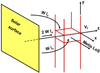 |
Fig. 1. Geometry of the 2D model. The prominence is approximated by an isothermal and isobaric horizontal slab (drawn in red) placed at certain height above the solar surface. Here, WI0 is the disk-center specific intensity of the Lα multiplied by the geometrical dilution factor, W. |
The slab is located at a height, H, above the solar surface and is illuminated by the incident solar radiation differently from the bottom and sides. From below, irradiation from the solid angle encompassing the whole solar disk as visible from the height H was used. The irradiation from both sides is half of that from bottom, that is, only half of the solid angle makes a contribution. No illumination from above was assumed because the radiation in hydrogen lines and continua from the hot solar corona is quite negligible, compared to incidental radiation from the solar disk.
Macroscopic velocities of the prominence as a whole were also considered in the model. Overall, CMEs and embedded prominence flux ropes can move in various directions, however, for the purposes of demonstration in this work, we restricted ourselves only to strictly vertical upward motion (along z) with the flow velocity, Vf. Due to such flows, the DDE significantly affects the Lα output radiation calculated by the code for fast-moving material with upward velocities of several hundreds km s−1, as previously shown by Heinzel & Rompolt (1987). We note that recent results from Peat et al. (2024) demonstrate the importance of the non-vertical component of the flow velocity vector on DDE. We note that at low velocities, say up to 50 km s−1, and low temperatures (i.e., a narrow Gaussian absorption profile), we can get slight Doppler brightening due to the reversal of the Lα chromospheric profile (shown in Fig. 2).
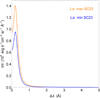 |
Fig. 2. Maximum and minimum Lα half profile of the incident radiation during solar cycle 23 according to Gunár et al. (2020). Note: 1 Å corresponds to a Doppler shift of roughly 250 km s−1. |
Realistic irradiation of the slab from the solar surface can also significantly influence the results of the model, as already demonstrated by Gunár et al. (2020), Gunár & Heinzel (2024). These authors also showed that the Lα emission from the chromosphere changes with the solar cycle and so, they developed a method to reconstruct the chromospheric emission in hydrogen lines for any desired phase of the selected solar cycle using the Laboratory for atmospheric and space physics Interactive Solar IRradiance Datacenter (LISIRD) composite Lα index (Machol et al. 2019). During solar cycle 23, the variation between the minimum and maximum Lα irradiation is remarkable, reaching 48% (as shown in Fig. 2). Therefore, for testing the influence of the solar-cycle phase on results of our modeling, we used two extreme cases for the incident radiation, minimum and maximum pertinent to this solar cycle. For both cases, we used the Lα reference profiles from Gunár et al. (2020) and the reference profiles of the higher Lyman lines from Warren et al. (1998). These profiles were adapted to each phase of the solar cycle using the method of Gunár et al. (2020).
Although we decided to use a horizontal 2D model, which may approximate a vertically expanding flux tube, the same MALI 2D code can easily be used for a vertically oriented tread. The presentation of such models would require too much attention to cover in this work, however, the authors can be contacted for access to a particular simulation. Vertical filaments were considered by Heinzel & Anzer (2001) in quiescent prominences, but mostly vertically moving eruptive prominences are better fitted by a horizontal rope. However, at a given height, the radiation output from both horizontal and vertical threads will be similar at the central regions.
3. Grid of models
We computed a large grid of isothermal and isobaric models using the 2D non-LTE MALI code and incident radiation from minimum and maximum of the solar cycle 23 (referred to here as the minimum and maximum). We focus on models relevant to the Metis coronagraph on board Solar Orbiter, which conducts simultaneous observations in the UV Lα line (121.6 nm ± 10 nm) and in VL (580–640 nm) at heights between 0.7 R⊙ and ∼9 R⊙ above the solar surface, depending on the distance between Solar Orbiter and the Sun.
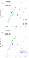 |
Fig. 3. Integrated intensity of the Lα line as function of the line-center optical thickness for a given height (4 R⊙) and thickness (10 000 km). Different flow velocities are indicated by symbols. Upper panel: Same, but for different temperatures (marked in color). Lower panel: Same, but for different gas pressures (marked in color). |
Each model is characterized by its kinetic temperature, T, gas pressure, p, the effective thickness of the slab, microturbulent velocity, Vt, flow velocity, and the height above the solar surface. For the input parameters of the 2D code, we assumed typical values known from the observations, ranging from cold, dense, and static prominences (Labrosse et al. 2010) to hot, low-density, and fast-moving eruptive prominences (Gopalswamy et al. 2015; Heinzel et al. 2016; Jejčič et al. 2017; Susino et al. 2018). We chose five different temperatures and gas pressures, four characteristic effective thicknesses, one microturbulent velocity, four different flow velocities, and four different heights relevant for Metis observations. Table 1 shows all the parameters that enter into the MALI code. In total, we obtained 1600 models for each minimum and maximum irradiation.
All input parameters used in the code. There are 1600 models for each incident radiation.
The relevant output parameters are the integrated intensity of the Lα line, ELα, together with its synthetic profiles and the optical thickness, τLα, in the line center. Meanwhile, the electron density, ne, the atomic level populations, and all excitation and ionization rates were calculated for the 5-level plus continuum hydrogen atom model. Although the code uses the 5-level plus continuum model, only the Lα transition and the integrated VL emission are relevant for Metis coronagraph observations and, thus, they are discussed in the next section. Other hydrogen radiation properties can be easily extracted from simulations.
4. Results
Our results are presented as plots showing correlations between various physical parameters and the prominence radiation output in the Lα and VL. All the following correlation plots are shown during the minimum and for a characteristic height of 4 R⊙ above the solar surface. We also chose a reference LoS thickness of the eruptive prominence structure of 10 000 km. In the following plots, all densities and rates are taken at the slab center.
Figure 3 shows the integrated intensity emitted in the Lα line as function of the optical thickness in the line center. This is a critical piece of information for analyzing the Metis data because if the observed line intensity indicates the optically thin structure, we can then safely use a simple scattering model, instead solving the transfer equation. Models for all pressures and temperatures are shown at height of 4 R⊙ and the effective thickness of 10 000 km. Both panels show the same plot. In the upper panel, the temperature is indicated by colors. In the lower panel, the pressure is indicated by colors. The cool prominence plasma at 10 kK and 20 kK is optically thick with values of the thickness between 100 and 106 and the ELα is between 10 and 107 erg s−1 cm−2 sr−1 for the selected effective thickness of 10 000 km. Meanwhile, hot prominence plasma with the temperature of 50 kK and above can become optically thin with the Lα intensity less than 10 erg s−1 cm−2 sr−1 for a selected LoS thickness. The upper panel shows that at a given temperature, the integrated intensity of the Lα line is proportional to the optical thickness. From the lower panel, we see that the higher the gas pressure, the higher the Lα emission and its optical thickness.
Nonetheless, ELα also depends on the height above the solar surface and effective thickness, as shown in Fig. 4. To illustrate this in a more optimal way, we plot here models for all pressures and two representative flow velocities 0 and 300 km s−1, indicated by the relevant symbols. The left panels refer to models with a temperature of 20 kK and right panels to models with a temperature of 100 kK. The upper panels display how the ELα versus τLα depends on the effective thickness (marked in colors) for models with the height of 4 R⊙. The higher the effective thickness, the stronger Lα intensity and larger optical thickness. The lower panels show how ELα versus τLα depends on the height (marked with colors) for models with the effective thickness of 10 000 km. We note that the height determines the illumination from the solar surface via the dilution factor, which decreases with height.
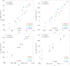 |
Fig. 4. Same plot as in Fig. 3, but for two representative flow velocities 0 and 300 km s−1, indicated by the symbols. Left panels show the results at a temperature of 20 kK and right panels at 100 kK. The upper panels show the same plot for the effective thickness dependence for a given height of 4 R⊙. Different thicknesses are indicated by different colors. The lower panels show the height dependence at a given thickness of 10 000 km. Different heights are indicated by the colors. |
Figure 5 shows the correlation between the integrated intensity emitted in the Lα line and the flow velocity. For an improved illustration, we selected three temperatures (from cool to hot) of prominence structures (indicated by colors) and two extreme gas pressures (indicated by the symbols). The plot clearly shows that ELα decreases with Vf at low pressure for all three temperatures due to the DDE. Yet at high pressure, ELα(Vf) is practically constant for any temperature.
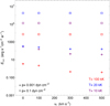 |
Fig. 5. Lα emission versus flow velocity for three selected temperatures covering the cold and hot structures in colors and two extreme values of the gas pressures in symbols for an improved representation at a height of 4 R⊙ and effective thickness of 10 000 km. |
The Lα spontaneous emission follows previous excitation either by the local Lα radiation field (this process is called scattering) or by an inelastic collision of the hydrogen atom with a free electron. These two contributions to the Lα emission are usually called the scattering and collisional components, respectively, as discussed by Susino & Bemporad (2016). For substantial velocities of eruptive prominences, the radiative component is affected by the DDE, (see Kohl & Withbroe 1982; Heinzel & Rompolt 1987; Peat et al. 2024). The radiative component is proportional to the Lα radiative excitation rate per atom R12, while the collisional component is proportional to the collisional rate per atom. These rates are defined by Eq. (1). Then total number of excitations per sec and per unit volume is n1[R12 + C12], where n1 is the number density of hydrogen atoms in the ground state. Ratio between the radiative component and the collisional component of the Lα line as a function of electron density is expressed as
 (1)
(1)
where B12 is the Einstein coefficient for radiative excitation,  is the mean intensity of the local Lα radiation weighted by the absorption profile and integrated over the whole line and Ω(T) is the rate of collisional excitation per one electron. This ratio is shown in Fig. 6. In cool prominence structures (T ≤ 20 kK), the ratio is proportional to the electron density (gas pressure) at a given temperature. The ratio is above 100, which implies that the resonant scattering dominates over the collisional excitation rate. A slow decrease in the ratio with ne at a given temperature is observed in hot prominence plasma (T ≥ 50 kK) up to ne < 3 ⋅ 108 cm−3 and for Vf < 100 km s−1. However, for larger flow velocities the ratio increases with ne all the time. When the ratio is around 1, both radiative and collisional excitation components are comparable and must be taken into account. It is only at T ≥ 80 kK that the ratio for fast-moving structures falls below 1 when the collisional component outweighs the radiative one. The DDE is noticeable up to ne < 3 ⋅ 108 cm−3 and Vf < 100 km s−1. Only at 20 kK the ratio is not sensitive to DDE. From Eq. (1), this ratio seems to be inversely proportional to ne, but our correlation, at least at lowest temperatures, shows the opposite. This is related to a dependence of
  on the emission measure, as we show later. Also, at low densities, we see the effect of Doppler dimming, which acts on the radiative rate only.
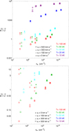 |
Fig. 6. Upper panel: Ratio between the radiative and collisional excitation rates in the Lα transition as a function of the electron density at height of 4 R⊙ and effective thickness of 10 000 km. The temperatures are represented by colors and flow velocities by symbols. Lower panel: Same plot for zoomed region at lower ratios. |
Figure 7 shows the ratio of the photoionization and collisional ionization rates from the hydrogen ground state versus the electron density for different temperatures (colors) and flow velocities (symbols). The ratio changes drastically with temperature. At 10 kK, the photoionization plays a dominant role as we know from studies of cool prominences, while at 20 kK both contributions are comparable (see also Heinzel et al. 2024). For hot prominence plasmas at T ≥ 50 kK the ratio is far below unity and the collisional ionization rate dominates over the photoionization one. At 100 kK the ratio decreases with increasing ne and at all other temperatures the ratio decreases with increasing ne up to about ne ∼ 109 cm−3 and then begins to increase with ne. This could be the effect of saturation of the internal radiation field in the Lyman continuum for thick structures. We note that at high temperatures, the collisional ionization equilibrium is a reasonable approximation (e.g., Susino & Bemporad 2016), but in cooler structures, the photoionization will dominate.
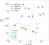 |
Fig. 7. Ratio between the photoionization rate and the collisional ionization rate from the hydrogen ground state, as a function of the electron density at height of 4 R⊙ and effective thickness of 10 000 km. The temperatures are represented by colors and the flow velocities by symbols. At high temperatures, R1k is fixed by the incident Lyman-continuum radiation, while the collisional rate is proportional to the electron density. |
The ionization degree versus electron density is shown in Fig. 8 for selected temperatures and flow velocities. We note that here the ionization degree is defined as i = np/nH, where np is the proton number density and nH is the total hydrogen density. At T = 10 kK the modeled plasma is weakly ionized with the ionization degree between 0.1 and 0.2 (0.5 for the models with the lowest pressure of 0.001 dyn cm−2). At 20 kK, the plasma is already almost completely ionized, with the ionization degree of about 0.9. At higher temperatures, it is practically fully ionized.
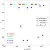 |
Fig. 8. Ionization degree as a function of the electron density at height of 4 R⊙ and effective thickness of 10 000 km. The temperatures are represented by colors and the flow velocities by symbols. |
The relative contribution of Balmer and Lyman continuum photoionizations to electron density is shown in Fig. 9. Here, DDE plays a role at low densities. For cool prominence structures, the ratio is about one, which means that both continua contribute in a similar way (see also Heinzel et al. 2024). For hot prominences, however, the ratio is much smaller than one and, in this case, the Lyman continuum photoionization dominates.
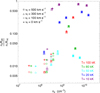 |
Fig. 9. Relative contribution of the Balmer and Lyman continuum photoionizations to the electron density at height of 4 R⊙ and effective thickness of 10 000 km. The temperatures are represented by colors and the flow velocities by symbols. |
Figure 10 shows a detailed radiative balance in Lα transition. Optically thick points lie on the dashed line, meaning that the Lα absorption is equal to the Lα emission. Optically thin points deviate from the dashed line and the radiative balance is not achieved for these points at the slab center.
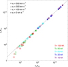 |
Fig. 10. Lα absorption versus Lα emission at height of 4 R⊙ and effective thickness of 10 000 km. The temperatures are represented by colors and the flow velocities by symbols. For comparison, the dashed line shows the position at which the ratio between the two is equal to one. |
The comparison between the integrated intensity, emitted in the Lα line and the emission measure defined as EM= ne2Deff is shown in Fig. 11. At a given temperature, the Lα integrated intensity is proportional to the emission measure. A similar behavior was found in case of the hydrogen Hα line (Gouttebroze et al. 1993). However, in case of Lα the explanation of such a correlation will be different and we will discuss it in a next paper, where we plan to use this relation for analysis of Metis Lα data.
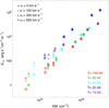 |
Fig. 11. Integrated intensity of the Lα line as a function of the emission measure (EM = ne2Deff) at a height of 4 R⊙ and effective thickness of 10 000 km for given temperatures (colors) and flow velocities (symbols). |
Figure 12 shows how Lα emission versus EM varies with height for two representative flow velocities (0 and 300 km s−1) at T = 20 kK (upper panel) and T = 50 kK (lower panel). At higher flow velocities, the relationship practically does not dependent on height and the relationship between the two is proportional. For a static structure, the relationship is height-dependent.
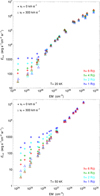 |
Fig. 12. Integrated intensity of the Lα line as function of the emission measure for all pressures, effective thicknesses at two representative flow velocities (symbols) and for all heights (colors), at T = 20 kK (upper) and T = 50 kK (lower). |
Since Metis simultaneously observes in Lα and VL channels, Fig. 13 shows the Lα emission over VL emission as a function of electron density. We can see that at a given temperature and given flow velocity, the integrated intensity emitted in the Lα line is proportional to the VL emission. We note that the VL emission is largely due to Thomson scattering of the incident disk radiation by free prominence electrons (see Heinzel et al. 2023). For structures located in the Metis PoS we have
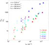 |
Fig. 13. Integrated intensity of the Lα line over VL emission as function of electron density at height of 4 R⊙ and effective thickness of 10 000 km for all temperatures (colors) and flow velocities (symbols). |
 (2)
(2)
where σT = 6.65 × 10⁻²⁵ cm2 is the Thomson cross section and Jtot = ∫νf(ν) J(ν) dν is integrated over Metis VL broadband filter between 580 and 640 nm. Here, f(ν) is the Metis filter transmittance curve and  is the mean intensity of the incident solar radiation, taking into account the frequency-dependent continuum limb darkening (Cox 2000) as shown in Table 2.
Mean intensity of the incident solar radiation relevant for Metis. J(ν, h) is in units of 10−7 erg s−1 cm−2 sr−1 Hz−1.
At a given temperature, the Lα integrated intensity provides an estimate of the emission measure, while the VL channel gives us the column density of prominence electrons. When combined together, we can derive both ne and Deff, similarly to what was proposed by Jejčič & Heinzel (2009), who used the combination of Hα and VL. We already started to apply this novel method to several eruptive prominences analyzed by Russano et al. (2024).
The relative error of the cyclic variation of the Lα emission during the maximum and minimum with electron density is shown in Fig. 14 at a height of 4 R⊙ and effective thickness of 10 000 km. Two representative flow velocities 0 and 300 km s−1 are shown by symbols and two temperatures 10 kK and 80 kK by colors. Since the difference in Lα illumination during the maximum and minimum is 48%, the difference in ELα is between 0.5% and 40% – depending on the speed of the moving structure.
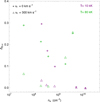 |
Fig. 14. Relative deviation of Lα emission during solar minimum and maximum versus electron density at height of 4 R⊙ and effective thickness of 10 000 km for two representative temperatures (color-coded) and for two flow velocities (symbol-coded). |
5. Discussion and conclusions
Various correlations between prominence radiation properties and plasma parameters presented in this paper should help observers interpret the Metis data. We have produced a large grid of 2D models: 1600 models for each type of external illumination (at the minimum and maximum of the solar cycle). This grid can be used for a quantitative analysis of Metis observations and, specifically, for Lα data, which indicate a non-negligible optical thickness of the prominence. Optically thin cases have been studied already using SOHO/UVCS observations, but the optically thick Lα problem is still challenging. Our correlations are aimed at providing a physical insight into radiation and plasma conditions, but they are limited to the choice of correlation plots (noting that our models are parametrized by six input parameters; see Table 1). Looking at several eruptive prominences observed by Metis in 2021 (Russano et al. 2024), we see that very low Lα intensities, ranging from 0.0065 to 0.2589 erg s−1 cm−2 sr−1, indicate (using our plots) that we are dealing with optically thin plasmas at relatively high temperatures and very low gas pressures. Also, the analysis of an eruptive prominence observed by SOHO/UVCS at points P1 and P2 (Heinzel et al. 2016) is consistent with our relations. Using our correlations, we can estimate whether the eruptive structure is optically thin or thick as well as which processes are relevant for plasma ionization and for excitation of the Lα transitions: photoionization versus collisional ionization and radiative versus collisional excitation (i.e., the radiative and collisional component of the Lα source function).
Using the electron density and the geometric thickness of the slab, we can compute the VL emission within the Metis channel, which is mainly due to Thomson scattering on prominence electrons. However, as demonstrated by Heinzel et al. (2023) the signal in VL channel can be significantly contaminated by the emission in helium D3 line, namely, at low temperatures. Finally, for the analysis of a particular observation, the authors of this paper can be contacted to run the MALI2D code under specific conditions.
Data availability
Tables with the physical parameters that are important for analyzing and interpreting the Metis data. These tables have been created for two extreme cases of the prominence illumination during the minimum and maximum of solar cycle 23. The tables can be accessed at https://zenodo.org/records/14884715.
Acknowledgments
S.J. acknowledges the support from the Slovenian Research Agency No. P1-0188. P.H., S.G. and S.J. acknowledge support from the grant 25-18282S of the Czech Science Foundation and from the project RVO:67985815 of the Astronomical Institute of the Czech Academy of Sciences. P.H. acknowledges support by the program ‘Excellence Initiative – Research University’ for years 2020-2026 at University of Wroclaw, project no. BPIDUB.4610.96.2021.KG. P.S. acknowledges support from the project VEGA 2/0043/24 of the Science Agency. S.J., P.S., and P.H. benefit from the discussions of the ISSI BJ Team “Solar eruptions: preparing for the next generation multi-waveband coronagraphs”. We thank the anonymous referee for useful comments and suggestions that helped to improve the paper.
References
- Andretta, V., Bemporad, A., De Leo, Y., et al. 2021, A&A, 656, L14 [NASA ADS] [CrossRef] [EDP Sciences] [Google Scholar]
- Antonucci, E., Romoli, M., Andretta, V., et al. 2020, A&A, 642, A10 [NASA ADS] [CrossRef] [EDP Sciences] [Google Scholar]
- Ciaravella, A., & Raymond, J. C. 2008, ApJ, 686, 1372 [NASA ADS] [CrossRef] [Google Scholar]
- Ciaravella, A., Raymond, J. C., Fineschi, S., et al. 1997, ApJ, 491, L59 [NASA ADS] [CrossRef] [Google Scholar]
- Cox, A. N. 2000, Allen’s Astrophysical Quantities (New York: AIP Press; Springer) [Google Scholar]
- Curdt, W., Tian, H., Teriaca, L., & Schühle, U. 2010, A&A, 511, L4 [NASA ADS] [CrossRef] [EDP Sciences] [Google Scholar]
- Fineschi, S., Naletto, G., Romoli, M., et al. 2020, Exp. Astron., 49, 239 [Google Scholar]
- Fontenla, J., Reichmann, E. J., & Tandberg-Hanssen, E. 1988, ApJ, 329, 464 [Google Scholar]
- Gopalswamy, N. 2015, in Solar Prominences, eds. J. C. Vial, & O. Engvold, Astrophys. Space Sci. Lib., 415, 381 [CrossRef] [Google Scholar]
- Gouttebroze, P., Heinzel, P., & Vial, J. C. 1993, A&AS, 99, 513 [NASA ADS] [Google Scholar]
- Gunár, S., & Heinzel, P. 2024, A&A, 687, A231 [NASA ADS] [CrossRef] [EDP Sciences] [Google Scholar]
- Gunár, S., Schwartz, P., Schmieder, B., Heinzel, P., & Anzer, U. 2010, A&A, 514, A43 [NASA ADS] [CrossRef] [EDP Sciences] [Google Scholar]
- Gunár, S., Schwartz, P., Dudík, J., et al. 2014, A&A, 567, A123 [NASA ADS] [CrossRef] [EDP Sciences] [Google Scholar]
- Gunár, S., Schwartz, P., Koza, J., & Heinzel, P. 2020, A&A, 644, A109 [EDP Sciences] [Google Scholar]
- Heinzel, P., & Anzer, U. 2001, A&A, 375, 1082 [NASA ADS] [CrossRef] [EDP Sciences] [Google Scholar]
- Heinzel, P., & Rompolt, B. 1987, Sol. Phys., 110, 171 [NASA ADS] [CrossRef] [Google Scholar]
- Heinzel, P., Gouttebroze, P., & Vial, J. C. 1987, A&A, 183, 351 [Google Scholar]
- Heinzel, P., Susino, R., Jejčič, S., Bemporad, A., & Anzer, U. 2016, A&A, 589, A128 [NASA ADS] [CrossRef] [EDP Sciences] [Google Scholar]
- Heinzel, P., Jejčič, S., Štěpán, J., et al. 2023, ApJ, 957, L10 [NASA ADS] [CrossRef] [Google Scholar]
- Heinzel, P., Gunár, S., & Jejčič, S. 2024, Phil. Trans. R. Soc. London Ser. A, 382, 20230221 [Google Scholar]
- Jejčič, S., & Heinzel, P. 2009, Sol. Phys., 254, 89 [NASA ADS] [CrossRef] [Google Scholar]
- Jejčič, S., Susino, R., Heinzel, P., et al. 2017, A&A, 607, A80 [NASA ADS] [CrossRef] [EDP Sciences] [Google Scholar]
- Kohl, J. L., & Withbroe, G. L. 1982, ApJ, 256, 263 [Google Scholar]
- Kunasz, P., & Auer, L. H. 1988, J. Quant. Spectr. Rad. Transf., 39, 67 [NASA ADS] [CrossRef] [Google Scholar]
- Labrosse, N., Heinzel, P., Vial, J. C., et al. 2010, Space Sci. Rev., 151, 243 [Google Scholar]
- Machol, J., Snow, M., Woodraska, D., et al. 2019, Earth Space Sci., 6, 2263 [Google Scholar]
- Peat, A. W., Osborne, C. M. J., & Heinzel, P. 2024, MNRAS, 533, L19 [NASA ADS] [CrossRef] [Google Scholar]
- Russano, G., Andretta, V., De Leo, Y., et al. 2024, A&A, 683, A191 [NASA ADS] [CrossRef] [EDP Sciences] [Google Scholar]
- Rybicki, G. B., & Hummer, D. G. 1991, A&A, 245, 171 [NASA ADS] [Google Scholar]
- Schwartz, P., Gunár, S., & Curdt, W. 2015, A&A, 577, A92 [NASA ADS] [CrossRef] [EDP Sciences] [Google Scholar]
- Susino, R., & Bemporad, A. 2016, ApJ, 830, 58 [Google Scholar]
- Susino, R., Bemporad, A., Jejčič, S., & Heinzel, P. 2018, A&A, 617, A21 [NASA ADS] [CrossRef] [EDP Sciences] [Google Scholar]
- Vial, J.-C. 1982, ApJ, 253, 330 [NASA ADS] [CrossRef] [Google Scholar]
- Vial, J. C., & Engvold, O. 2015, in Solar Prominences, (Springer International Publishing Switzerland), Astrophys. Space Sci. Lib., 415 [Google Scholar]
- Vial, J. C., Ebadi, H., & Ajabshirizadeh, A. 2007, Sol. Phys., 246, 327 [NASA ADS] [Google Scholar]
- Warren, H. P., Mariska, J. T., & Wilhelm, K. 1998, ApJS, 119, 105 [Google Scholar]
- Wilhelm, K., Curdt, W., Marsch, E., et al. 1995, Sol. Phys., 162, 189 [Google Scholar]
All Tables
All input parameters used in the code. There are 1600 models for each incident radiation.
Mean intensity of the incident solar radiation relevant for Metis. J(ν, h) is in units of 10−7 erg s−1 cm−2 sr−1 Hz−1.
All Figures
|
Fig. 1. Geometry of the 2D model. The prominence is approximated by an isothermal and isobaric horizontal slab (drawn in red) placed at certain height above the solar surface. Here, WI0 is the disk-center specific intensity of the Lα multiplied by the geometrical dilution factor, W. |
| In the text | |
|
Fig. 2. Maximum and minimum Lα half profile of the incident radiation during solar cycle 23 according to Gunár et al. (2020). Note: 1 Å corresponds to a Doppler shift of roughly 250 km s−1. |
| In the text | |
|
Fig. 3. Integrated intensity of the Lα line as function of the line-center optical thickness for a given height (4 R⊙) and thickness (10 000 km). Different flow velocities are indicated by symbols. Upper panel: Same, but for different temperatures (marked in color). Lower panel: Same, but for different gas pressures (marked in color). |
| In the text | |
|
Fig. 4. Same plot as in Fig. 3, but for two representative flow velocities 0 and 300 km s−1, indicated by the symbols. Left panels show the results at a temperature of 20 kK and right panels at 100 kK. The upper panels show the same plot for the effective thickness dependence for a given height of 4 R⊙. Different thicknesses are indicated by different colors. The lower panels show the height dependence at a given thickness of 10 000 km. Different heights are indicated by the colors. |
| In the text | |
|
Fig. 5. Lα emission versus flow velocity for three selected temperatures covering the cold and hot structures in colors and two extreme values of the gas pressures in symbols for an improved representation at a height of 4 R⊙ and effective thickness of 10 000 km. |
| In the text | |
|
Fig. 6. Upper panel: Ratio between the radiative and collisional excitation rates in the Lα transition as a function of the electron density at height of 4 R⊙ and effective thickness of 10 000 km. The temperatures are represented by colors and flow velocities by symbols. Lower panel: Same plot for zoomed region at lower ratios. |
| In the text | |
|
Fig. 7. Ratio between the photoionization rate and the collisional ionization rate from the hydrogen ground state, as a function of the electron density at height of 4 R⊙ and effective thickness of 10 000 km. The temperatures are represented by colors and the flow velocities by symbols. At high temperatures, R1k is fixed by the incident Lyman-continuum radiation, while the collisional rate is proportional to the electron density. |
| In the text | |
|
Fig. 8. Ionization degree as a function of the electron density at height of 4 R⊙ and effective thickness of 10 000 km. The temperatures are represented by colors and the flow velocities by symbols. |
| In the text | |
|
Fig. 9. Relative contribution of the Balmer and Lyman continuum photoionizations to the electron density at height of 4 R⊙ and effective thickness of 10 000 km. The temperatures are represented by colors and the flow velocities by symbols. |
| In the text | |
|
Fig. 10. Lα absorption versus Lα emission at height of 4 R⊙ and effective thickness of 10 000 km. The temperatures are represented by colors and the flow velocities by symbols. For comparison, the dashed line shows the position at which the ratio between the two is equal to one. |
| In the text | |
|
Fig. 11. Integrated intensity of the Lα line as a function of the emission measure (EM = ne2Deff) at a height of 4 R⊙ and effective thickness of 10 000 km for given temperatures (colors) and flow velocities (symbols). |
| In the text | |
|
Fig. 12. Integrated intensity of the Lα line as function of the emission measure for all pressures, effective thicknesses at two representative flow velocities (symbols) and for all heights (colors), at T = 20 kK (upper) and T = 50 kK (lower). |
| In the text | |
|
Fig. 13. Integrated intensity of the Lα line over VL emission as function of electron density at height of 4 R⊙ and effective thickness of 10 000 km for all temperatures (colors) and flow velocities (symbols). |
| In the text | |
|
Fig. 14. Relative deviation of Lα emission during solar minimum and maximum versus electron density at height of 4 R⊙ and effective thickness of 10 000 km for two representative temperatures (color-coded) and for two flow velocities (symbol-coded). |
| In the text | |
Current usage metrics show cumulative count of Article Views (full-text article views including HTML views, PDF and ePub downloads, according to the available data) and Abstracts Views on Vision4Press platform.
Data correspond to usage on the plateform after 2015. The current usage metrics is available 48-96 hours after online publication and is updated daily on week days.
Initial download of the metrics may take a while.