| Issue |
A&A
Volume 699, July 2025
|
|
|---|---|---|
| Article Number | A111 | |
| Number of page(s) | 23 | |
| Section | Stellar structure and evolution | |
| DOI | https://doi.org/10.1051/0004-6361/202553727 | |
| Published online | 01 July 2025 | |
Probing the cores of subdwarf B stars: How they compare to cores in helium core-burning red giants
1
Instituto de Astrofísica e Ciências do Espaço, Universidade do Porto, CAUP, Rua das Estrelas, PT4150-762 Porto, Portugal
2
Departamento de Física e Astronomia, Faculdade de Ciências, Universidade do Porto, Rua do Campo Alegre 687, PT4169-007 Porto, Portugal
3
Leiden Observatory, Leiden University, PO Box 9513 NL-2300 RA Leiden, The Netherlands
⋆ Corresponding author: This email address is being protected from spambots. You need JavaScript enabled to view it.
Received:
11
January
2025
Accepted:
30
April
2025
Abstract
The mixing of material from stellar convective cores into their adjacent radiative layers has been a matter of long-standing debate. Pulsating subdwarf B stars offer excellent conditions to advance our understanding of this problem. In this work we use a model-independent approach to infer information about the cores of three subdwarf B stars and compare it with similar inferences from an earlier analysis of red giants in the helium core-burning phase. This is achieved by fitting an analytical description of the gravity-mode pulsation periods to pulsation data collected by the Kepler satellite. From the fits we infer the reduced asymptotic period spacings and the amplitude and position of sharp structural variations associated with chemical discontinuities in the stellar interiors. Our results indicate the presence of sharp structural variations with similar properties in all three stars, located near the edge of the gravity-mode propagation cavity and likely associated with the C-O/He transition. We find that these structural variations differ systematically from those of helium core-burning red giant stars, having larger amplitudes and being located at a larger buoyancy radius. This suggests that chemical mixing beyond the adiabatically stratified core into the radiatively stratified layers may be more extensive in subdwarf B stars than in helium core-burning red giants. Alternatively, the stratification of the mixing region beyond the adiabatically stratified core may differ significantly between the two types of stars. The model-independent constraints set on the structural variations inside these three stars are the first of a kind and will be key to enhancing the modelling of layers adjacent to stellar convective cores and to testing non-canonical stellar evolution channels leading to the formation of hot subdwarf stars.
Key words: stars: evolution / stars: interiors / stars: oscillations
© The Authors 2025
 Open Access article, published by EDP Sciences, under the terms of the Creative Commons Attribution License (https://creativecommons.org/licenses/by/4.0), which permits unrestricted use, distribution, and reproduction in any medium, provided the original work is properly cited.
This article is published in open access under the Subscribe to Open model. This email address is being protected from spambots. You need JavaScript enabled to view it. to support open access publication.
1. Introduction
Subdwarf B (sdB) stars are compact, hot objects with a helium-burning core and a thin hydrogen-rich envelope that is incapable of sustaining nuclear reactions (see Heber 2016, for a review). With about half a solar mass, they resemble stripped versions of low-mass helium core-burning red giant stars. Thus comparative asteroseismic studies of sdB stars and helium core-burning red giants hold the potential to significantly advance our understanding of the processes leading to the formation of sdB stars. They are often observed to be in close binaries, mostly with a white dwarf companion and thought to be a product of binary evolution involving a common-envelope phase. However, different processes, including stellar-planet interactions, stellar mergers, and non-standard single star evolution, are also evoked as possible channels to form sdB stars (Clausen & Wade 2011; Heber 2016; Zhang et al. 2017; Rui & Fuller 2024).
A significant fraction of sdB stars exhibit either acoustic (p) or gravity (g) modes, and some exhibit both (e.g. Baran et al. 2023; Uzundag et al. 2024). Unlike the mixed modes observed in red giants, the purely acoustic or gravity nature of pulsations observed in sdB stars simplifies the development of inference methodologies. Of particular interest, the seismic data on several sdB stars have revealed signatures of sharp structural variations in the g-mode part of the pulsation spectra (Østensen et al. 2014; Baran et al. 2017; Uzundag et al. 2017). These are thought to be associated with strong chemical gradients inside the star, located at the transition between the carbon-oxygen-enriched mixed core and the helium mantle (C-O/He transition) and between the helium mantle and the thin hydrogen-rich envelope (He/H transition). While both chemical transitions impact the pulsation periods, their relative seismic importance depends on the range of periods observed, as well as on the mixing processes taking place near the core (Ghasemi et al. 2017; Guyot et al. 2025). Moreover, the seismic impact of the chemical transitions depends on their sharpness; in particular, on how the scale of the transition compares to the local wavelength of the observed modes. This has been illustrated by Charpinet et al. (2014) for a sdB model, where the authors show that the seismic signature of the relatively wide He/H transition decreases significantly as the pulsation periods increase. The same phenomena was addressed in Cunha et al. (2015) and is discussed further in Sect. 3.2 of this work.
Asteroseismic studies of sdB pulsators have so far been based on forward modelling (e.g. Ghasemi et al. 2017; Uzundag et al. 2021; Baran & Sanjayan 2023) recurring to either stellar evolution codes or static structural models (Charpinet et al. 2000, 2002; Guyot et al. 2025). However, the pure nature (gravity or acoustic) of the modes observed in these stars makes them key targets to employ model-independent asteroseismic techniques. This is particularly true for the study of sharp structural variations such as the ones discussed above.
Structural variations on scales comparable to or shorter than the local wavelength of the modes (hereafter, glitches) have been the focus of many seismic studies. Some of the tools for the direct inference of the properties of these glitches without recourse to stellar models date from the earlier days of helioseismology, and have seen diverse applications over the years (see Cunha 2020, for a review). However, the variational approach adopted in the context of the sun and other p-mode pulsators to derive the analytical formulation needed to fit the seismic data and make the intended inferences is usually not adequate for studies of g-mode pulsators. This is because the perturbations induced on the g-mode pulsation periods by glitches in the buoyancy frequency are rarely small. The same is true in the study of buoyancy glitches in mixed-mode pulsators.
When the glitch impact on the pulsation periods is not small, perturbations to the pulsation periods may be derived instead by matching the wave solutions on each side of the glitch. This approach was used by Cunha et al. (2015, 2019, 2024) to derive analytical expressions for the period and period-spacing perturbations induced by buoyancy glitches of different shapes in g- and mixed-mode pulsators. These tools have recently been successfully applied in the analysis of glitches in a sample of low-mass, helium core-burning red giant stars by Vrard et al. (2022). In this work we apply them to the study of three sdB pulsators in which evidence of glitch signatures has been detected, and compare the properties inferred for their glitches with those inferred in the work by Vrard et al. (2022) in the analysis of the helium core-burning red giant stars.
The remainder of the paper is organized as follows. In Sect. 2, we present the published pulsation periods used in this work and their sources. In Sect. 3, we introduce the analytical model for the seismic signature of structural glitches and discuss the role of each model parameter. In Sect. 4, we describe the fitting methods adopted and the results from the fits to the data on each star. In Sect. 5, we discuss our inferences in light of the combined analysis of the three stars and compare them to the results from earlier analyses of the helium core-burning red giant stars. Finally, in Sect. 6, we summarize our main conclusions.
2. Data
We consider three stars for our case study; namely, KIC 10553698A, studied by Østensen et al. (2014) based on Kepler short-cadence data collected over nine quarters in the period between Q8 and Q17, EPIC 211779126, studied by Baran et al. (2017) based on short-cadence data collected during the K2 Campaign 5, and KIC 10001893, studied by Uzundag et al. (2017) based on Kepler short-cadence data collected continuously between Q6 and Q17.2. Of relevance for our study are the high radial order g modes. These are listed in Tables A.1 and A.2 for KIC 10553698A, A.3 for EPIC 211779126, and A.4 for KIC 10001893, in appendix A. The tables show the mode radial order, n, degree, l, and period, P, according to the information provided in the original studies, as well as the reduced periods, defined as  . For EPIC 211779126 and KIC 10001893, no obvious multiplets are observed in the power spectrum in the range of periods considered in this study. However, in the case of KIC 10553698A, multiplets are observed. In Table A.1 we list estimates of the central components of these multiplets, reproduced following the discussion in section 3.8 of Østensen et al. (2014) and the authors’ Figure 10. The original list of mode periods in the range of relevance, including the individual multiplet components listed in their work, is reproduced in Table A.2. In a few cases, the three works report period spacings that were not computed from the modes listed in their tables. Estimates of the respective periods are also given in the respective tables.
3. Periods and period spacing models in the presence of glitches
In the absence of fast rotation and other agents that may break the spherical symmetry of the star, an asymptotic analysis predicts that high-radial-order gravity modes of the same degree are equally spaced in period (Tassoul 1980). Written in terms of the reduced period, this spacing is
 (1)
(1)
Here, 𝒲g1 is the size of the g-mode propagation cavity expressed in terms of the buoyancy frequency, N, as
 (2)
(2)
where r is the distance from the stellar centre, and r1 and r2 are the inner and outer turning points of the cavity, respectively. Moreover, if the star has a convective core, in the asymptotic regime the reduced periods can be written as
 (3)
(3)
for a series of natural numbers, k, where Πs, min is the first of a series of equally spaced reduced periods.
We note that the reduced periods in Eq. (3) do not depend on mode degree. In stars with a radiative core, N2 is positive in the innermost layers, approaching zero only at the centre, as N ∝ r. As a consequence, the reduced periods depend on the mode degree. However, this is not expected in sdB stars, because their cores are unstable to convection, preventing g modes from propagating into the centre of the star. In these stars the inner turning point, r1, is located at the edge of the convective core, here defined as the border of the adiabatically stratified region, hence including any extra mixing regions resulting from processes that maintain an adiabatic thermal stratification (see, e.g. Guyot et al. 2025, for a discussion). Moreover, while the outer turning point, r2, may generally depend on the mode degree and oscillation period, changes to the outer turning point have a negligible impact on the integral defined in Eq. (2), and hence on the reduced periods. That is corroborated by the data on the three stars considered in this work. In fact, the reduced periods of dipole and quadrupole modes are generally closely aligned in these stars and there is no evidence for a dependence of the asymptotic reduced period spacing on the oscillation period.
3.1. Glitch signature
The equally spaced sequence reported above is modified in the presence of structural variations occurring on scales smaller or comparable to the local wavelength (hereafter, named glitches) located within the propagation cavity. To describe the glitch position, we introduce the degree-independent buoyancy radius,
 (4)
(4)
and the degree-independent buoyancy depth,  . In all cases, we characterise the glitch position in terms of the buoyancy distance measured from the closest turning point.
For a single glitch, the periods are represented by (Cunha et al. 2024)
 (5)
(5)
where Πs represents the unperturbed reduced periods (i.e. without the glitch effect) of a hypothetical model in which the integral of N/r within the g-mode cavity is the same as in the glitch model, and ϕ represents the phase perturbation caused by the glitch. Moreover, the glitch-induced phase depends on the functional form of the glitch. Here, two options shall be considered, namely a step-like function and a Gaussian-like function (see Figure 1 of Cunha et al. (2019) for illustration). For the case of the a step-like glitch, the phase is given by
![Mathematical equation: $$ \begin{aligned} \phi =\mathrm{arccot}\left[-\frac{2}{A_{\rm st}\sin \left(2\theta \right)}-\cot \theta \right], \end{aligned} $$](/articles/aa/full_html/2025/07/aa53727-25/aa53727-25-eq8.gif) (6)
(6)
while in the case of a Gaussian-like glitch, the phase is given by
![Mathematical equation: $$ \begin{aligned} \phi =\mathrm{arccot}\left[\frac{1}{A_{\rm G}{ f}_{\omega }^{\Delta _{\rm g}}\sin ^2\theta }-\cot \theta \right], \end{aligned} $$](/articles/aa/full_html/2025/07/aa53727-25/aa53727-25-eq9.gif) (7)
(7)
where, fωΔg = ω−1exp(−2Δg2ω−2) and ω is the angular frequency. Here, Ast and AG are always positive and provide a measure of the amplitude of the glitch located at r = r⋆, in the case of the step-like and Gaussian-like glitch, respectively. Moreover, Δg is a measure of the width of the Gaussian-like glitch and
 (8)
(8)
depending on whether the glitch is located in the inner half ( /𝒲g < 0.5) or outer half (
 /𝒲g > 0.5) of the propagation cavity, respectively. We note that in the above, a ⋆ means that the quantities are taken at r = r⋆. Finally, δ is an extra phase that absorbs the impact of the approximations performed in the analysis near the turning points of the modes and is not related to the glitch shape. This extra parameter also accommodates the impact in Eq. (6) of changing the sign of the structural variation (e.g., a local drop versus a local increase in buoyancy frequency) in the case of a step-like glitch. This sign change will introduce a π/2 variation in the parameter δ, without changing the expression itself. By symmetry, this also means that the expression for the phase, ϕ, is independent of the side of the cavity in which the glitch is located, insofar as the correct definition for the buoyancy position of the glitch (buoyancy radius or depth, as discussed above) is taken (see Cunha et al. 2024, for details).
Finally, we note that Eq. (6) is periodic, with a period given by
 (9)
(9)
for ( /𝒲g < 0.5) and (
 /𝒲g > 0.5), respectively. That implies that the signature of a step-like glitch on the reduced periods will be strictly repeated with this periodicity. In the case of a Gaussian-like glitch, inspection of Eq. (7) shows that the glitch signature also changes periodically with the same periodicity, but its amplitude is simultaneously modified due to the frequency-dependent function, fωΔg.
The analysis followed by these authors can be expanded to consider additional buoyancy glitches, so long as these are sufficiently apart to guarantee that the asymptotic solutions are valid in between them (see Appendix B). In the case of two glitches, the reduced periods are given by
 (10)
(10)
where φ represents the phase perturbation caused by the additional glitch. As in the case of the first glitch, the functional form of φ is given either by Eq. (6) or Eq. (7), depending on whether it is modelled by a step or a Gaussian function, respectively. Moreover, if the two glitches are located in opposite sides of the g-mode cavity, θ is given by the left and right expression of Eq. (8), for the inner and outer glitch, respectively. Finally, the expression for the period spacings, defined by the difference in the reduced period of modes of consecutive radial order ΔΠ = Πn + 1 − Πn, is given by
![Mathematical equation: $$ \begin{aligned} \frac{\Delta \Pi }{\Delta \Pi _{\rm as}}\approx \left[1+\frac{\Delta \Pi _{\rm as}}{\pi }\left(\frac{\mathrm{d}\phi }{\mathrm{d}\Pi }+\frac{\mathrm{d}\varphi }{\mathrm{d}\Pi }\right)\right]^{-1}, \end{aligned} $$](/articles/aa/full_html/2025/07/aa53727-25/aa53727-25-eq17.gif) (11)
(11)
where the derivatives of the phases, ϕ and φ, can be computed numerically or analytically (cf. Cunha et al. 2019).
3.2. Model parameters
When fitting the analytical expression (11) to data, the number and type of parameters depend on the number of glitches and glitch shapes. The common parameter to all cases is the asymptotic reduced period spacing, ΔΠas. Then, for each glitch we have the buoyancy radius,  , (or the buoyancy depth, 𝒲g⋆) at the glitch position, and the fudge parameter δ. Depending on the shape of the glitch, we have also either a dimensionless amplitude, Ast (step-like glitch) or an amplitude and a width, AG and Δg, respectively (Gaussian-like glitch). When fitting the analytical expression for the periods (10), there is an additional parameter that represents the smallest reduced period in the fitted range, Πs, min.
Figure 1 illustrates the impact on the period spacings from changing the physical parameters of a single-glitch model, as well as from changing the glitch shape. The reference model, shown in panel a., considers ΔΠas = 300 s and a step-like glitch with Ast = 10,  = 0.008 rad/s (or Πsig = 2467 s) and δ = 1.3. These parameters imply that the relative position of the glitch in the cavity for the reference model is
  ≈ 0.12.
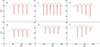 |
Fig. 1. Continuous reduced period spacing signal predicted by the analytical model (Eq. (11)), considering a single step-like glitch (Eq. (6)) and varying the model parameters one at a time (red line). The horizontal dotted line marks the asymptotic reduced period spacing value ΔΠas. Panel a.: Reference case with ΔΠas = 300 s, Ast = 10, |


-
The asymptotic reduced period spacing, ΔΠas, controls the value around which the period spacing deviations take place. In addition, it acts as a scaling factor for the glitch-induced perturbations, as expected from Eq. (10). This impact is illustrated in panel b. where the value has been decreased to ΔΠas = 250 s.
-
The glitch position,
 (or 𝒲g⋆, for a glitch in the outer cavity), controls the separation between the extrema of the period-spacing function, with larger values implying smaller separations. This is shown in panel c., where the glitch was moved slightly closer to the centre of the cavity, with
  = 0.01 rad/s (
 ≈ 0.15; Πsig = 1974 s).
 -
The glitch amplitude, Ast for a step-like glitch, controls the extent of the period-spacing deviation from ΔΠas, with a smaller amplitude (Ast = 5; panel d.) showing shallower humps and dips. When the amplitude is sufficiently small, the variation in the reduced period spacing becomes sinusoidal and symmetrical about the value of ΔΠas.
-
Changes in the phase, δ, induce only a horizontal translation of the reduced period spacings (not shown in Fig. 1).
-
Changing the shape of the glitch impacts the dependence of the reduced period-spacing perturbations on the reduced periods. While for a step-like glitch the extrema of the perturbations are independent of the reduced period (panels a. to d.), in a Gaussian-like glitch the period dependence is clear (panels e. and f.). This dependence is controlled by the function fωΔg appearing in Eq. (7). When the width of the glitch, Δg, tends to zero, the period dependence is dominated by the factor 1/ω, and the extrema of the perturbations increase with the reduced period (panel e.); otherwise, the dependence is dominated by the exponential factor and the extrema of the perturbations decrease as the reduced period increases (panel f.). The latter behaviour results from the fact that as the reduced period increases, the local wavelength of the wave decreases, eventually becoming smaller than the width of the structural variation. At that point, the structural variation ceases to be a glitch and the glitch-induced perturbation disappears.
4. Inference of glitch properties
The reduced period spacings are shown for the three stars in the top panels of Figs. 2, 4, and 5, respectively. In all three stars, reduced period-spacing dips are observed, consistent with the signature of structural glitches. We note that the reduced period spacings for the l = 1 and l = 2 modes are generally aligned, as expected asymptotically for a star with a spherically symmetric equilibrium and a convective core (e.g., Cunha et al. 2007). Exceptions to this alignment may indicate problems with the identification of the modes, as noted in the original works. These cases are discussed further below.
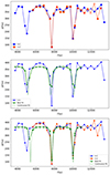 |
Fig. 2. KIC 10553698A reduced period spacings as a function of the reduced period. Each reduced period spacing is plotted at the mid point between the reduced periods used in its computation. The parameters for the best fit solutions are given in Appendix C. Top panel: observed reduced period spacings for l = 1 (blue) and l = 2 (red) in the full range. The discrete observed values are joined by straight lines to guide the eye. Open symbols indicate reduced period spacings that cannot be computed from the frequencies listed in the original table (see section 3.8 of Østensen et al. 2014, for details). Middle panel: the best fit solution to the l = 1 reduced period spacings at reduced periods smaller than 11 100 s, for the case of a one step-like glitch (green) (case A). The continuous analytical solution is represented by the dashed line, while the filled stars indicate the values of the solution at the reduced periods corresponding to the locations of the observations. Bottom panel: similar to middle panel, but including in the fit both the l = 1 (blue) and the l = 2 (red) modes at reduced periods smaller than 11 100 s (case B). |
To fit the period-spacing model to the data and infer the glitch properties, a dynamic nested sampling algorithm (Higson et al. 2018) was implemented using the dynesty Python package. The likelihood was assumed to be Gaussian and given by the following expression,
 (12)
(12)
where χ2 is defined as
 (13)
(13)
N is the number of data points to be fitted, and 𝒬data and 𝒬model are, respectively, the data and respective model quantity being compared (in the present case, the period spacings, ΔΠ). In addition to the parameters implicit in the analytical model for the periods and period spacings, equation (13) contains the error, σ, which is also taken to be a free parameter. We note that no observational errors were provided in the original works from which the data used here were extracted, so using the observational errors in the definition of the likelihood was not an option. In any case, we anticipate that the typical observational errors – connected to the pulsation spectra resolution, mode amplitude variability, and so on – are negligible compared with the errors associated with the model predictions. In fact, while the analytical expressions are expected to capture the essence of the glitch impact on the pulsation periods, it is likely that in most cases they are insufficiently accurate to model the data within typical observational errors. This is due both to the approximations inherent to the analysis performed to derive the analytical expressions and to the fact that glitches in real stars are not expected to be perfectly described by step, Gaussian or Dirac δ functions. Consequently, the introduction of σ as a parameter enables us not only to proceed without having access to the observational errors but also to quantify the ability of our models to reproduce the data.
We ran the nested sampler algorithm with 250 live points and a burn-in set to one-tenth of the total chain length, using multiple bounding ellipsoids and setting the sampling method to be random walks. Uniform priors were used for all parameters within the parameter space explored. From these, we extracted the parameters corresponding to the maximum of the likelihood, as well as the median parameters of the posterior distribution and associated 68 percent confidence intervals.
In addition, for KIC 10553698A we fitted the reduced periods using a step-like glitch (i.e., Eqs. (5)–(6)) and different options for the data selection, as detailed in Sect. 4.1. This was motivated by the presence of multiplets in the g-mode range in this star, which makes the identification of the central peaks needed to construct the period spacings particularly difficult (Østensen et al. 2014). The fits to the reduced periods followed the procedure described in Cunha et al. (2024), where the data were fitted through a Markov Chain Monte Carlo (MCMC) method using the emcee Python package and the likelihood was also assumed to be Gaussian (Eqs. (12)–(13) with 𝒬 = Π) and the priors were taken to be uniform within the parameter space explored.
For each star, several scenarios were tested. The motivation for the choice of glitch models and the results from the fits for each star are discussed in the following subsections.
4.1. KIC 10553698A
Two modulations appear to be present in the reduced period spacings of KIC 10553698A, with different amplitudes and scales, (Fig. 2, top panel). The first, of a larger scale, is characterised by three significant dips, while the second, of shorter scale, has a comparatively small amplitude. Although both modulations seem to be present and in phase in the modes of degree l = 1 and l = 2 up to a reduced period of Π ∼ 11 100 s, the short-scale modulation on the two mode degrees becomes out of phase for reduced periods larger than that value. As discussed by Østensen et al. (2014), amplitude variability and rotational splitting make the identification of the modes difficult in this star. This is particularly so at high radial orders (large periods) where the peaks in the multiplets become increasingly apart in period. For this reason, the authors state that the offsets seen in the reduced period spacings computed from modes of different degree are likely not of physical origin. With this in mind, for KIC 10553698A we disregarded the reduced period spacings for periods above 11 100 s when fitting our analytical model. Moreover, given that the amplitude of the short-scale modulation is similar in magnitude to the differences in the reduced period spacings for l = 1 and l = 2 modes, we disregarded also that modulation when choosing the model to fit. Therefore, we considered a one glitch model aimed at fitting the dominant larger-scale modulation observed in the reduced period spacings of KIC 10553698A. The absence of a significant change in the amplitude of the glitch signature, which shows variations that can be well explained by the limited sampling by the data, points to a sharp transition, such as the one that may be expected in the C-O/He transition (cf. Sect. 1). Thus, we assumed a step-like glitch, which provides the simplest possible representation of the data, with a minimum number of model parameters.
Two fits were performed to the reduced period spacings. The first considers only the modes of l = 1, which cover all observed dips (case A). Fitting to the l = 1 data thus ensures that all dips are given the same weight. The best-fit solution for this case (i.e. the solution with maximum likelihood) is shown in the middle panel of Fig. 2 (green stars), along with the observed l = 1 reduced period spacings (blue circles). Here, and in all following figures, the solutions are shown only in the range of reduced period spacings where the fits are performed. The solution shows that the model captures well the three-dip structure seen in the observed period spacing. This is corroborated by the posterior distribution for the glitch position shown in Fig. C.1 (in appendix C). The latter shows that the model parameter that measures the buoyancy radius at the glitch position, which more directly affects the distance between period-spacing dips, is well constrained. The fact that the extremes of the dips are not well reproduced by the best-fit solution (cf. Fig. 2, middle panel) is not surprising, as the dips are narrow and not well sampled by the discrete data. As a consequence, the fraction of data points contributing to constraining the dips is relatively small. In fact, considering that the phase, δ, simply induces a horizontal translation of the analytical solution, it is possible to see from the continuous solution for the best-fit model (shown by the dashed green line) that the extremes of the model dips will change significantly if a slightly different value of the phase is taken for a glitch of equal position and amplitude.
Unlike the glitch position, the glitch amplitude is not well constrained, as seen by inspection of the respective posterior distribution (Fig. C.1). The reason is again related to the limited sampling of the dips in the reduced period spacings. In the analytical model, the glitch amplitude controls the minima of the period-spacing dips, which decrease further as the amplitude increases. However, no matter how extreme the dips predicted by the continuous model are, a slight change in the phase will result in the dips being sampled away from their minima, mimicking the signal of a smaller amplitude glitch. As a result, in a poorly sampled case the glitch amplitude is never well constrained at the higher values. Moreover, at the lower end of the amplitude posterior distribution, the large errors implied by the simplicity of the model (which assumes a single step-like function) also limit the constraining power of the data regarding the glitch amplitude due to the appearance of solutions corresponding to a flat reduced period spacing (i.e., no glitch) with values smaller that the preferred solution (i.e., outside the 68 percent interval for ΔΠas). These results are in line with earlier discussions in the literature in the context of both buoyancy and acoustic glitches, where it is systematically found that the glitch parameter whose inference is most reliable is the glitch position (Mazumdar et al. 2014; Cunha et al. 2024). The median and associated 68 percent uncertainty intervals for the physical parameters inferred from the fit are summarized in the first row of Table 1 (case A).
Seismic and glitch properties of KIC 10553698A derived from fits of a step-like glitch model to the data.
The second fit to the reduced period spacings of KIC 10553698A adopted the same model but considered both modes of degree l = 1 and l = 2 up to Π = 11 100 s (case B). The best-fit solution and the posterior distributions for the model parameters are shown in Fig. 2 (bottom panel) and Fig. C.2, respectively. Here, the increase in the number of data points leads to a better representation of the extremes of the second and third period-spacing dips, at the expense of having the first dip less well reproduced by the model. We note that the Gaussian-glitch model also predicts equally spaced dips in the reduced period spacing (cf. Fig. 1). Thus, adopting instead a Gaussian-glitch model would not solve the small mismatch between the equally spaced dips predicted by the model and the slightly uneven observed spacing. The mismatch may have an observational origin, if one of the modes near the first dip was misidentified due to the complexity of the oscillation spectra discussed above. Alternatively, it could be an indication that the glitch has a more complex struture or that the model becomes less adequate at lower periods.
The impact of the additional (and consistent) l = 2 data is clearly reflected in the posterior distribution for the glitch amplitude. In fact, the added weight of the data around the second and third dips removes some of the degeneracy of the model solutions corresponding to large glitch amplitudes. Moreover, the fact that the model representation of the data is improved when adding the l = 2 modes (as seen from the error parameter distribution), makes solutions of very low amplitude significantly less likely than when fitting only the l = 1 modes. These results show that if enough data are available, the glitch amplitude can be reasonably constrained, despite the large uncertainties. Comparison of the median values for the physical parameters in the two cases (Table 1, cases A and B) shows that the inferred parameters are consistent within the uncertainties, with the second fit setting more stringent constraints, as expected.
As was mentioned earlier, KIC 10553698A shows a series of multiplets, or partial multiplets, in the g-mode period range. These add to the complexity of its oscillation spectra and may compromise the identification of modes of similar degree and azimuthal order, needed to determine the reduced period spacings. For this reason, it is of interest to understand how the results from fitting directly the oscillation periods, without assuming prior knowledge of the azimuthal orders, compare with those from fitting the period spacings assuming prior knowledge of the central peaks in each multiplet.
The results obtained from fitting the periods and the period spacings constructed from the same periods should be consistent. To verify that this is the case, we started by fitting the reduced periods smaller than 11 100 s listed in Table A.1 for the l = 1 and l = 2 modes, used to construct the reduced period spacings fitted in the previous exercise. The reduced periods were fitted with the same step-like glitch model as before, now expressed through Eqs. (5)–(6), and the median values for the inferred parameters are listed in Table 1 (case C). The glitch properties inferred from this fit agree within the errors with the results of the fit to the reduced period spacings constructed from the same data (case B). The best-fit model from the fit to the reduced periods is shown in the Echelle diagram displayed in the left panel of Fig. 3, constructed in the manner described in Cunha et al. (2024).
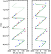 |
Fig. 3. KIC 10553698A echelle diagrams displaying the data for l = 1 (blue) and l = 2 (red) modes, along with the best fit model for the case of a one step-like glitch (green). The continuous analytical solution is represented by the full line in the reduced periods’ range in which the fit was performed and by a dotted line in the range not considered in the fit. Left panel: Fit to l = 1 and l = 2 modes’ reduced periods smaller than 11 100 s (case C). The data used in this fit were also used to construct the reduced period spacings for case B in Table 1, whose fit is shown in the bottom panel of Fig. 2. Right panel: Fit to l = 1 and l = 2 modes’ reduced periods in the full range (up to n = 34) extracted from Table A.2 (case E). When several modes are listed for a given radial order and degree (or for the same trapped mode), one single mode was picked randomly (see text for details). |
Next, we relaxed the assumptions made regarding the identification of the central peaks in each multiplet, used in the construction of the period spacing series (Østensen et al. 2014). To that end, we considered the full list of oscillation periods published by the authors in the same range of radial orders as before (Table A.2). For each radial order and degree, we randomly chose one of the values whenever more than one period was listed. Restricting the data to reduced periods smaller than 11 100 s, we then performed a fit to the reduced periods using Eqs. (5) and (6). The exercise was repeated three times, so that the list of reduced periods fitted each time was slightly different, due to the random choice of the peak in each multiplet. For all inferred parameters, the variance in the median was found to be much smaller (always less than 3 percent) than the errors in the respective parameter, which implies that the choice of peak in each multiplet does not affect the inferences in a significant way. The means of the parameters (i.e., of the medians and respective errors) inferred from the fits to the three different datasets selected in the way described above are also listed in Table 1 (case D).
Finally, we also relaxed the restriction on the range of reduced periods to be fitted, considering the full list of periods in Table A.2 and randomly choosing a reduced period from each multiplet, as before. The best-fit model for this case is illustrated in the Echelle diagram displayed on the right panel of Fig. 3 and the inferred parameters are also listed in Table 1 (case E). Here we see that the reduced asymptotic period spacing and glitch amplitude agree within the errors with those inferred in cases A to D, but the glitch position is off by about 2–4 times the respective uncertainty, depending on the case. This is a consequence of the additional data fitted (i.e., the reduced periods larger than 11 100 s) and not of the random selection of the peaks in the multiplets or of the option to fit the reduced periods rather than the reduced period spacings.
4.2. EPIC 211779126
The reduced period spacings of EPIC 211779126 (top panel of Fig. 4) show two dips between 5000 s and 8000 s, followed by smaller amplitude variations. The modes in this star also exhibit amplitude variability, a fact emphasized by Baran et al. (2017) with a word of caution when the authors say that the frequencies they list should be considered approximate. In fact, the reduced period spacings computed from the l = 1 and l = 2 data are partially in phase, particularly in the second reduced period-spacing dip and near the high end of the reduced periods, but a mismatch is seen in the first dip and at intermediate values of the reduced periods. In particular, the separation between the dips in the reduced period spacings is different in the l = 1 and l = 2 mode series. This is not expected from asymptotic analysis, and is not seen in pulsation calculations of sdB models, as far as we are aware (Charpinet et al. 2002; Ostrowski et al. 2021). While we do not exclude the possibility that the differences in the two series may be real, our glitch model uses the asymptotic solutions on either side of the glitch and, thus, predicts similar results for the modes of different degree, for a given structural glitch. For that reason, we fitted the modes of different degree separately, adopting a one-glitch model, and then accessed the impact from the differences observed in the l = 1 and l = 2 data on the glitch inferences. Given our choice of a single-glitch model, we aimed only at reproducing the dominant dips in the reduced period spacings.
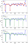 |
Fig. 4. EPIC 211779126 reduced period spacings as a function of the reduced period. Each reduced period spacing is plotted at the mid point between the reduced periods used in its computation. The parameters for the best fit solutions are given in Appendix C. Top panel: Observed reduced period spacings for l = 1 (blue) and l = 2 (red) modes. The discrete values are joined by straight lines to guide the eye. Symbols meaning as in the top panel of Fig. 2. Middle panel: Best-fit solution (green) to the l = 1 data (blue) for the case of a one step-like glitch (case F). The continuous analytical solution is represented by the dashed line, while the filled stars indicate the values of the solution at the reduced periods corresponding to the locations of the observations. Bottom panel: Same as middle panel but for the case of a one Gaussian-like glitch (green) (case H). |
Concerning the representation of the glitch, we considered two cases, namely a step and a Gaussian function. The motivation for comparing these two cases comes from the fact that no significant dips are observed beyond ∼7500 s. There are several possible explanations for this fact. On the one hand, the absence of the dips can be related to the observations themselves. With dips as extreme as the ones observed in this star, where the difference between the periods of the trapped mode and the mode that follows are as small as 20 s, and the amplitude variability already discussed, one needs to consider the possibility that some modes in the range of periods considered here were not detectable in the power spectrum. Missing modes between those used to construct the period spacings shown in the top panel of Fig. 4 would lead to the absence of what would otherwise be additional dips. On the other hand, the absence of additional dips can be real. If the structural variation is not sufficiently sharp, at larger periods its width may be significantly larger than the local characteristic scale of the wave, in which case the structural variation will no longer act as a glitch. In this case, the signature of the structural variation on the period spacings will decrease with period, tending to zero as the structural variation becomes a smooth background variation from the perspective of the wave, as discussed in Sect. 3.2 (see also discussions in Charpinet et al. 2014; Cunha 2020). That is precisely what is predicted when the glitch is modelled by a Gaussian function. Finally, the glitch may be sharp, but the conditions necessary for the occurrence of visible trapping are not always satisfied. This case, as well as the cases in which it may be difficult to detect all modes in a given region of the power spectrum, is best modelled by a step function.
The best fits to the l = 1 modes are shown in Fig. 4 for a model with a step-like glitch (middle panel, case F) and a model with a Gaussian glitch (bottom panel, case H). Both models capture the two-dip structure, but adjust differently to a comparably flatter reduced period spacing at higher reduced periods, as expected. In the case of the step-like glitch, the reduced period-spacing dips of the best-fit continuous solution are not always revealed by the observed modes, whereas in the Gaussian-like model, the dips disappear because the amplitude of the glitch signature decreases with reduced period.
The posterior distributions for the model parameters and respective medians and 68 percent uncertainties are shown in Figs. C.3 (step-like glitch model) and C.4 (Gaussian-like glitch model) and Table 2 (cases F and H). As before, in both cases we see that the glitch position is well constrained, while the glitch amplitude is not. Moreover, comparison of the median values of the glitch position inferred in the two cases shows agreement within the uncertainties, as expected from the fact that both glitch models are capable of capturing well the two dips observed in the reduced period spacings.
Seismic and glitch properties of EPIC 211779126 derived from fits of step-like and Gaussian glitch models to the data.
Fits to the l = 2 modes were performed with the same models (cases G and I). The best-fit models adjust to the data similarly well as they did when fitting to the l = 1 modes, so we refrain from showing the plots here. However, in Table 3, we provide a measure of the quality of the fitting for the four cases (two for l = 1 and two for l = 2) for comparison. As the error, σ, was left as a free parameter, we cannot use χ2 defined by equation (13) directly to compare the quality between the fits performed to different sets of data or with different glitch models. Instead, we first re-normalised the χ2 obtained for each fit by multiplying it by the value of σ2 obtained for the best-fit model and then dividing the result by a reference value, namely σ402 = (40 s)2. We then divided the result by N − m, where N is the number of fitted data points and m the number of parameters in the model, to compute the corresponding reduced value, χR402, which we show in Table 3.
Quality of the fits performed to the reduced period spacings of EPIC 211779126.
The medians and 68 percent uncertainties for the parameters inferred from the fits to the l = 2 data are also shown in Table 2 (cases G and I). As was expected, the position of the glitch inferred when fitting to the l = 2 data differs from that inferred when fitting to the l = 1 data (in that the value of  is smaller for l = 2) because the dips in the reduced period spacings are further apart in the l = 2 case.
4.3. KIC 10001893
The reduced period spacings of KIC 10001893 derived from the data of Uzundag et al. (2017) are shown in the top panel of Fig. 5. Three dips are observed for the l = 1 series of modes, but only two of these are covered by the l = 2 modes. As pointed out by the authors, the fact that a dip is observed simultaneously for both mode degrees is particular important in a star like this, in which no multiplets are seen. In fact, they consider the significance of the first trapped mode less convincing and stress that although other unidentified modes could be associated with trapped modes, the absence of multiplets prevents them from having a clear preference. With this in mind, in our analysis we considered two cases; namely, a fit to the region where the l = 1 and l = 2 reduced periods overlap and a fit to all data available, covering the three dips. In both cases we followed the same strategy as before and did not attempt to fit the short-scale variations observed in the reduced period spacings, which in the present case appear at low values of the reduced periods. Therefore, for the first fit we adopted a model with a single step-like glitch. However, for the second fit a single glitch model is not adequate. When considering the three dips in the upper panel of Fig. 5, we find that the distance between consecutive dips is too different to be adequately modelled by the impact of a single glitch, which predicts equally spaced dips in the reduced period spacings. Therefore, when fitting all l = 1 and l = 2 modes, we instead considered a model with two step-like glitches. These could hypothetically correspond to two different regions inside the star (e.g., associated with the CO/He and the He/H transitions).
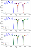 |
Fig. 5. KIC 10001893 reduced period spacings as a function of the reduced period. Each reduced period spacing is plotted at the mid point between the reduced periods used in its computation. The parameters for the best fit solutions are given in Appendix C. Top panel: Observed reduced period spacings for l = 1 (blue) and l = 2 (red) modes. The discrete values are joined by straight lines to guide the eye. Symbols meaning as in the top panel of Fig. 2. Middle panel: Best-fit solution (green) to the l = 1 (blue) and l = 2 (red) data in the range of periods where data on both mode degrees are available, for the case of a one step-like glitch (case J). The continuous analytical solution is represented by the dashed line, while the filled stars indicate the values of the solution at the reduced periods corresponding to the locations of the observations. Bottom panel: Same as middle panel but for the case of two step-like glitches fitted to all data displayed in the panel (green) (case K). |
The best-fit solutions obtained from the fits performed are shown in the middle panel (fit to the l = 1 and l = 2 overlap region) and bottom panel (fit to all data). Also, the median values of the model parameters and respective uncertainties are shown in Table 4. Although both cases capture well the reduced period spacing dips in the fitted regions, the solutions are significantly different. In the first case (single glitch; overlap region) the glitch position is such as to reproduce the separation between the second and third period-spacing dips. In the second case (two glitches; all data) one of the glitches is positioned such as to reproduce the first and third dips, while the other glitch reproduces the single dip in the middle, without predicting any additional dip within the observed range of reduced periods. Consequently, in this case both glitches are positioned at at buoyancy radius (or depth) smaller than the glitch inferred in the fit to the overlap region.
Seismic and glitch properties of KIC 10001893 derived from fits of a one step- and two step-like glitch models to the data.
Inspection of the posterior distributions for the model parameters presented in Figs. C.5 and C.6 emphasises further differences between the two fits. In the one-glitch fit to the overlap region, all parameters are well constrained, including the glitch amplitude. The constraining power to the amplitude in this case results from a combination of factors. Firstly, the data from the l = 1 and l = 2 modes is in excellent agreement and focused on the region of the dips, so the constraints around the dips being fitted are stringer than in all cases considered before. Secondly, the one-glitch model fits the data significantly better than in previous cases, as seen from the error distribution in Fig. C.5 (whose median value is ∼19 s, compared to median values ∼45 − 60 s in previous cases). In the two-glitch case, Fig. C.6 shows the difficulty in properly constraining the second glitch (the one labelled ‘out’ that reproduces the second period-spacing dip). This is expected, as all glitch positions closer to one of the edges of the buoyancy cavity than a given value are possible solutions. In this case, that value corresponds to the glitch position that would induce a signal with dips separated by as much as the range of reduced periods considered. This threshold induces the abrupt right-hand-side drop in the posterior distribution of ωg, out⋆ for the second glitch, which we arbitrarily take to be the one in the outer cavity (cf. Fig. C.6), to the left of which we observe a plateau of similarly good solutions.
5. Discussion
5.1. Glitch nature
The glitch properties inferred for the three stars in this study indicate that the same phenomenon is being observed in all cases. This is illustrated in Fig. 6 where we can see the similarity of the glitch positions and glitch amplitudes (albeit the latter inferred with large uncertainties). The figure shows also the asymptotic reduced period spacings for the three stars, confirming the overall similarity of their radiative inner structure. The cases illustrated for each star are identified on the x axis of the figure. For KIC10553698A (KIC1 in the figure), we show the fits to the reduced periods up to 11 100 s, the most reliable data range, as discussed in Sect. 4.1. Fitting all reduced periods listed in Tables A.2 leads to only a slightly smaller value of the glitch position. For KIC10001893 (KIC2), we show only the results from the fit with a one-glitch model, for consistency with the analyses shown for the other stars. The fit of the data assuming a two-glitch model leads to a very different solution, where neither glitch is located in a position comparable to that seen in the other stars. This reinforces the idea that the one-glitch model is likely more adequate to explain the data for this star, hence, that the characteristic periodicity of the glitch signature in KIC10001893 is given by the distance between two consecutive dips in the stars’ reduced period spacings. In this interpretation, the uneven separation between the three dips observed in the period spacings results either from a misidentification of the trapped mode in the oscillation spectrum, or potentially from the glitch shape being more complex than the adopted step function. In relation to the former possibility, Uzundag et al. (2017) point out that the significance of the first trapped mode they identify for l = 1, between n = 17 and n = 18, is less convincing than that of the second trapped mode, and that there are other unidentified peaks that could be associated with trapped modes but the lack of multiplets makes it difficult for the authors to make a definitive selection.
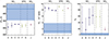 |
Fig. 6. Physical parameters inferred from the fits with a one step-like glitch model. The stars are identified in the top axis as KIC1=KIC10553698A, EPIC=EPIC211779126, and KIC2=KIC10001893 and the respective results are separated by a dash-dotted line. The labels in the x axis identify the case according to the results given in Tables 1, 2, and 4. From left to right, the panels show, with symbols and error bars, the median and respective 68 percent uncertainties, on the asymptotic reduced period spacing, degree-independent glitch buoyancy radius, and glitch amplitude, respectively. The blue line and shaded blue area in each panel show, respectively, the median and range of values found by Vrard et al. (2022) for the same parameters in the study of a sample of helium core-burning red giant stars. |
The fact that the period-spacing dips in two of the three stars (KIC10001893 and KIC10553698A) do not significantly depend on the reduced periods, indicates that the glitch is sharp. In the third star (EPIC211779126) only two dips are observed, followed by a long plateau in which the reduced period spacings vary only with small amplitude. This could be an indication of a wider structural variation which would cease to act as a glitch for the modes of longer period (shorter characteristic scale). However, comparison between fits to the data of this star with step-like and Gaussian-like glitch models do not necessarily corroborate that interpretation. In fact, the fits for the two cases have similar qualities (Table 3) and inspection of the middle and bottom panels of Fig. 4 seems to indicate that the step-like glitch provides a better representation of the flat top of the period spacings. Together with the fact that the glitch position inferred from the fits to the data of EPIC211779126 is similar to that inferred for the other two stars, we argue that it is more likely that the period-spacing signature in this star is produced by the same structural transition as in the other two stars.
When considering the nature of the structural transition that is causing the signature observed in the reduced period spacings, it is important to recall that the thermal and chemical stratifications of the layers adjacent to the convectively unstable core of sdB stars are still largely unknown. In this context, the interpretation of the glitch position needs to bear in mind that g modes do not propagate into the adiabatically stratified part of the core. Thus, the glitch location inferred from our fits is blind to those layers, measuring only the buoyancy distance from the edge of the convective core, i.e., the border of the adiabatically stratified region as defined in Sect. 3. Recently, Guyot et al. (2025) have studied the pulsation spectra of sdB models with different core properties illustrating the sensitivity of the period spacing modulation to the stratification of the core. Comparing the values of Πsig that we infer with the results from their models, it seems that the glitches in these stars are best compatible with the C-O/He transition in sdB stars with a low core-He abundance and a relatively small core mass. In addition, the data analysed here potentially hints at a slightly sharper glitch than the transition in their models, as their results show a smooth decrease in the depth of the period-spacing dips with increasing period. This typical characteristic of the signatures from non-sharp transitions is not evident in the observational data. However, with only three period-spacing dips it is impossible to establish the significance of this difference between the authors’ models and the observational data.
5.2. Comparison with glitches observed in helium core-burning red giants
Subdwarf B stars are likely the product of non-standard evolution involving the stripping of the outer layers of a star in the red giant branch. Therefore, it is important to investigate how the cores of helium core-burning red giant stars, which arise from standard stellar evolution, compare to those of sdB stars, which reach helium core burning through non-standard evolutionary channels. The inference of the core glitch properties in these stars provides the opportunity to address this question directly from the analysis of the data, i.e., in a way which is independent from our ability to build stellar evolution or static stellar models. With this in mind, in Fig. 6 we overplot in blue the range of asymptotic reduced period spacings, glitch locations, and glitch amplitudes derived by Vrard et al. (2022) for 23 helium core-burning red giants. The horizontal blue line marks the median of the respective quantities which were converted to their reduced form when relevant.
The difference in the results for the two samples is striking. In the case of the asymptotic reduced period spacings, it reflects an overall difference in the radiative interior of the two types of stars. In the case of the glitch amplitude, it could reflect a difference in the relative amplitude of the discontinuity in the buoyancy frequency at the chemical transition, or simply result from the finite width of the transition. In fact, the periods of the modes observed in the sdB stars are shorter, by a factor of ∼5, than the periods of mixed modes observed in helium core-burning red giants. Thus, a slow dependence of the amplitude of the glitch signature on the reduced periods, resulting from a hypothetical intrinsic width of the glitch, would lead to a much smaller amplitude of the glitch signature at the longer periods observed in the helium core-burning red giants than in the range of periods observed in sdB stars. Since both the helium core-burning red giant data and the sdB data were fitted with step-like glitch models that do not incorporate a period dependence of the glitch-signature amplitude, the hypothetical glitch width would be wrongly translated into a difference in the amplitudes inferred for the structural variations in the two types of stars.
However, perhaps the most interesting difference observed in the properties inferred for the sdB and the helium core-burning red giants concerns the glitch position. Due to its strict association with the periodicity of the glitch signature, this result is robust and cannot be explained by a change in the shape of the glitch. If the signature observed in the data of sdB and helium core-burning red giant stars is indeed associated with a transition close to the convective core, then the glitch position given in terms of the absolute quantity  provides a direct measurement of the integral of N/r from the edge of the convective core, where presumably the inner turning point of the modes is located, to the maximum extent of the chemical mixing into the radiative core (cf. Eq. (4)). According to our results, that extent is significantly different in the two types of stars.
6. Conclusions
In this work we used an analytical model developed in the works of Cunha et al. (2019, 2024) for g modes to directly infer information on structural glitches inside three sdB stars, without recourse to specific stellar models. Our main conclusions are as follows.
-
Despite their simplicity, in all three stars the analytical models capture well the most significant variations in the periods around the equally spaced asymptotic prediction.
-
According to the model inferences, the structural glitches inducing the observed period perturbations have similar properties in all three stars. They are consistent with sharp discontinuities located close to one of the turning points of the g-mode cavity, likely the C-O/He transition. A comparison with recent results from Guyot et al. (2025) favours a scenario in which these are evolved sdB stars with a low core-He abundance and a relatively small core mass.
-
The results indicate that the glitch properties in sdB stars are systematically different from those of glitches in helium core-burning red giants derived by Vrard et al. (2022). In particular, the sdB glitches are located at significantly larger buoyancy radii, indicating either a more extensive mixing region beyond the edge of the convective core or a different stratification of that mixing region.
Whether or not the differences found between the glitches in sdB and helium core-burning red giant stars can be explained by the adjustment of the stellar structure to the stripping of the outer layers is key to testing and understanding the evolution channels leading to the formation of sdB stars. That is best answered by simulations of the stellar structure and will be addressed in future work.
With the exception of the corner plots shown in appendix C, throughout this manuscript we use degree-independent buoyancy measurements rather than their degree-dependent counterparts used in earlier works by Cunha et al. (2015, 2019, 2024), for which only modes of l = 1 were considered. The relation between the two definitions is a  factor (e.g.,
  ).
).
Acknowledgments
This work has been supported by Fundação para a Ciência e Tecnologia FCT-MCTES, Portugal, through national funds by these grants UIDB/04434/2020 (DOI: 10.54499/UIDB/04434/2020), UIDP/04434/2020.FCT (DOI: 10.54499/UIDP/04434/2020) and 2022.03993.PTDC (DOI:10.54499/2022.03993.PTDC). MSC is funded by FCT-MCTES by the contract with reference 2023.09303.CEECIND/CP2839/CT0003 (DOI:10.54499/2023.09303.CEECIND/CP2839/CT0003). AF acknowledges the funding from FEDER (through COMPETE2020 programme) and FCT under the project ‘BreakStarS’, attributed by CAUP with reference: CIAAUP-06/2022-BII.
References
- Baran, A., & Sanjayan, S. 2023, Acta Astron., 73, 21 [Google Scholar]
- Baran, A. S., Reed, M. D., Østensen, R. H., Telting, J. H., & Jeffery, C. S. 2017, A&A, 597, A95 [NASA ADS] [CrossRef] [EDP Sciences] [Google Scholar]
- Baran, A. S., Van Grootel, V., Østensen, R. H., et al. 2023, A&A, 669, A48 [NASA ADS] [CrossRef] [EDP Sciences] [Google Scholar]
- Charpinet, S., Fontaine, G., Brassard, P., & Dorman, B. 2000, ApJS, 131, 223 [Google Scholar]
- Charpinet, S., Fontaine, G., Brassard, P., & Dorman, B. 2002, ApJS, 139, 487 [Google Scholar]
- Charpinet, S., Brassard, P., Van Grootel, V., & Fontaine, G. 2014, in 6th Meeting on Hot Subdwarf Stars and Related Objects, eds. V. van Grootel, E. Green, G. Fontaine, & S. Charpinet, ASP Conf. Ser., 481, 179 [Google Scholar]
- Clausen, D., & Wade, R. A. 2011, ApJ, 733, L42 [NASA ADS] [CrossRef] [Google Scholar]
- Cunha, M. S. 2020, in Dynamics of the Sun and Stars; Honoring the Life and Work of Michael J. Thompson, eds. M. J. P. F. G. Monteiro, R. A. García, J. Christensen-Dalsgaard, & S. W. McIntosh, Astrophys. Space Sci. Proc., 57, 185 [NASA ADS] [CrossRef] [Google Scholar]
- Cunha, M. S., Aerts, C., Christensen-Dalsgaard, J., et al. 2007, A&A Rev., 14, 217 [Google Scholar]
- Cunha, M. S., Stello, D., Avelino, P. P., Christensen-Dalsgaard, J., & Townsend, R. H. D. 2015, ApJ, 805, 127 [NASA ADS] [CrossRef] [Google Scholar]
- Cunha, M. S., Avelino, P. P., Christensen-Dalsgaard, J., et al. 2019, MNRAS, 490, 909 [Google Scholar]
- Cunha, M. S., Damasceno, Y. C., Amaral, J., et al. 2024, A&A, 687, A100 [NASA ADS] [CrossRef] [EDP Sciences] [Google Scholar]
- Ghasemi, H., Moravveji, E., Aerts, C., Safari, H., & Vučković, M. 2017, MNRAS, 465, 1518 [Google Scholar]
- Gough, D. O. 2007, Astron. Nachr., 328, 273 [NASA ADS] [CrossRef] [Google Scholar]
- Guyot, N., Van Grootel, V., Charpinet, S., et al. 2025, A&A, 696, A13 [NASA ADS] [CrossRef] [EDP Sciences] [Google Scholar]
- Heber, U. 2016, PASP, 128, 082001 [Google Scholar]
- Higson, E., Handley, W., Hobson, M., & Lasenby, A. 2018, Stat. Comput., 29, 891 [Google Scholar]
- Mazumdar, A., Monteiro, M. J. P. F. G., Ballot, J., et al. 2014, ApJ, 782, 18 [NASA ADS] [CrossRef] [Google Scholar]
- Østensen, R. H., Telting, J. H., Reed, M. D., et al. 2014, A&A, 569, A15 [NASA ADS] [CrossRef] [EDP Sciences] [Google Scholar]
- Ostrowski, J., Baran, A. S., Sanjayan, S., & Sahoo, S. K. 2021, MNRAS, 503, 4646 [Google Scholar]
- Reed, M. D., Kawaler, S. D., Østensen, R. H., et al. 2010, MNRAS, 409, 1496 [NASA ADS] [CrossRef] [Google Scholar]
- Rui, N. Z., & Fuller, J. 2024, Open J. Astrophys., 7, 81 [NASA ADS] [CrossRef] [Google Scholar]
- Tassoul, M. 1980, ApJS, 43, 469 [Google Scholar]
- Uzundag, M., Baran, A. S., Østensen, R. H., et al. 2017, MNRAS, 472, 700 [CrossRef] [Google Scholar]
- Uzundag, M., Vučković, M., Németh, P., et al. 2021, A&A, 651, A121 [NASA ADS] [CrossRef] [EDP Sciences] [Google Scholar]
- Uzundag, M., Krzesinski, J., Pelisoli, I., et al. 2024, A&A, 684, A118 [NASA ADS] [CrossRef] [EDP Sciences] [Google Scholar]
- Vrard, M., Cunha, M. S., Bossini, D., et al. 2022, Nat. Commun., 13, 7553 [CrossRef] [Google Scholar]
- Zhang, X., Hall, P. D., Jeffery, C. S., & Bi, S. 2017, ApJ, 835, 242 [NASA ADS] [CrossRef] [Google Scholar]
Appendix A: Data
KIC 10553698A: observed periods used for cases A to D of Table 1 (source Østensen et al. 2014).
KIC 10553698A: observed periods used for case E identified in Table 1 in this work (source Østensen et al. 2014).
EPIC 211779126: observed periods used in this work (source Baran et al. 2017).
KIC 10001893: observed periods used in this work (source Uzundag et al. 2017).
Appendix B: Two-glitch model
Here we expand on the analysis presented in Cunha et al. (2019) to show how the eigenvalue condition derived for the one glitch model can be expanded to consider the case of two glitches, so far as they are sufficiently apart that the eigenfunction in between the glitches can be assumed to be well represented by the asymptotic solution. We take, as an example, the case of two step-like glitches, one on each side of the g-mode cavity. Other cases (e.g., for glitches with different shapes) can be derived following similar steps. Without loss of generality, we shall assume that N drops abruptly in the inner cavity and then increases abruptly, in the outer cavity. As discussed by Cunha et al. (2024), reverting the sign of these structural changes does not change the glitch-induced signature in the periods, so far as the inferred amplitude is restricted to be positive and its value is interpreted as ![Mathematical equation: $ A_{\mathrm{st}}^{\pm}=[N_{\mathrm{+}}/N_{\mathrm{-}}]_{r^\star}-1 $](/articles/aa/full_html/2025/07/aa53727-25/aa53727-25-eq89.gif) , where the subscripts + and − indicate the largest and the smallest of the two values of N at the discontinuity r⋆.
, where the subscripts + and − indicate the largest and the smallest of the two values of N at the discontinuity r⋆.
In the present case we then considered that N is well represented by
 (B.1)
(B.1)
with N varying by the positive amounts ΔN1 = Nin|r → r1−⋆ − Nmid|r → r1+⋆ and ΔN2 = Nout|r → r2+⋆ − Nmid|r → r2−⋆ at r = r1⋆ and r = r2⋆, respectively.
Our starting point is the wave equation A1 of Appendix A of Cunha et al. (2019). In terms of the variable  , where δp is the Lagrangian pressure perturbation, ρ is the density, g is the gravitational acceleration, and
  is a function of frequency and of the equilibrium structure [the f-mode discriminant defined by equation 35 of Gough (2007)], the equation resulting from the linear, adiabatic pulsation equations for the case of a spherically symmetric equilibrium under the Cowling approximation, can be written as
 (B.2)
(B.2)
where a prime represents a differentiation with respect to r. Given our focus on g modes, we approximate the radial wavenumber K as
 (B.3)
(B.3)
with L2 = l(l + 1) and ω the angular frequency of the mode.
The asymptotic solution satisfying the wave equation can be written in each region of the star as
 (B.4)
(B.4)
where  ,
,  , and
, and  are constants and φ, whose functional form is to be derived, accounts for the phase shift induced by the glitch located at r = r2⋆.
Next we define the glitch amplitudes:
Ast 1 = [(Kin−Kmid)/Kmid]r = r1⋆
Ast 2 = [(Kout−Kmid)/Kmid]r = r2⋆.
Imposing the continuity of Ψ and of its derivative at r = r1⋆ we find the eigenvalue condition
 (B.5)
(B.5)
We note that this condition is similar to the eigenvalue condition derived for mixed modes in the presence of a step-like glitch in the inner half of the g-mode cavity (Cunha et al. 2024), but φ is now to be interpreted as the phase shift induced by the outer glitch rather than the phase induced by the coupling with the p-mode cavity. Rewriting the first integral on right-hand-side of Eq. (B.5) in terms of the other two integrals and developing the expression one can write the eigenvalue condition as
 (B.6)
(B.6)
where ϕ is the phase induced by the glitch located at r = r1⋆ and is given by
 (B.7)
(B.7)
The functional form of the phase φ is derived by imposing the continuity of Ψ and of its derivative at r = r2⋆. This leads to the condition
 (B.8)
(B.8)
Developing the right-hand-side of Eq. (B.8) we then find that
 (B.9)
(B.9)
The fact that the two phases have the same functional form, which, in turn, is the same as that derived for a single step-like glitch in Cunha et al. (2019), results from our option to model both glitches with a step function in the example given here.
The eigenvalue condition expressed by Eq. (B.6) differs from equation 5 of Cunha et al. (2024) only in the addition of the extra phase φ introduced by the outer glitch. Moreover, it is mathematically equivalent to equation 36 of Cunha et al. (2015), despite the different meanings of the phase φ. The derivations from Eq. (B.6) of the expressions for the reduced periods (Eq. (10)) and reduced period spacings (Eq. (11)) in the presence two glitches, thus follow the exact same steps as in these earlier works and we do not repeat them here. Noting that except near the turning points, K ≈ LN/rω, we approximate the integrals in the definitions of ϕ and φ so that  and
and  , where δ accounts for the approximation made near the respective turning point. With this approximation, we recover the functional form for the step-like glitch ϕ and φ in the form given by Eq (6).
Appendix C: Model fits
Corner plots and best-fit models for the selection of fits discussed in the main text. Note that in the corner plots the glitch positions are expressed in terms of the degree-dependent buoyancy radius, ωg⋆, and depth,  , used in earlier works. To compare with the values provided for
  in the tables in the main text, the values of
  in the corner plots need to be divided by
  .
.
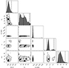 |
Fig. C.1. Posterior distributions for the model parameters resulting from the fit of the analytical model for one step-like glitch to the reduced period spacings of l = 1 of KIC 10553698A, for reduced periods smaller than 11100 s (case A). |
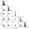 |
Fig. C.2. Posterior distributions for the model parameters resulting from the fit of the analytical model for one step-like glitch to the reduced period spacings of l = 1 and l = 2 of KIC 10553698A, for reduced periods smaller than 11100 s (case B). |
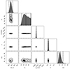 |
Fig. C.3. Posterior distributions for the model parameters resulting from the fit of the analytical model for one step-like glitch to the reduced period spacings of l = 1 of EPIC 211779126 (case F). |
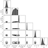 |
Fig. C.4. Posterior distributions for the model parameters resulting from the fit of the analytical model for one Gaussian-like glitch to the reduced period spacings of l = 1 of EPIC 211779126 (case H). |
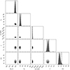 |
Fig. C.5. Posterior distributions for the model parameters resulting from the fit of the analytical model for one step-like glitch to the reduced period spacings computed from the l = 1 and l = 2 modes of KIC 10001893 in the region of periods where data on both mode degrees are available (case J). |
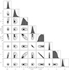 |
Fig. C.6. Posterior distributions for the model parameters resulting from the fit of the analytical model for two step-like glitches to all reduced period spacings computed from the l = 1 and l = 2 modes of KIC 10001893 (case K). |
Best model parameters for cases A and B in Table 1.
Best model parameters for cases C and E in Table 1.
Best model parameters for cases A and B in Table 2.
Best model parameters for case C and D in Table 2.
Best model parameters for cases A and B in Table 4.
All Tables
Seismic and glitch properties of KIC 10553698A derived from fits of a step-like glitch model to the data.
Seismic and glitch properties of EPIC 211779126 derived from fits of step-like and Gaussian glitch models to the data.
Seismic and glitch properties of KIC 10001893 derived from fits of a one step- and two step-like glitch models to the data.
KIC 10553698A: observed periods used for cases A to D of Table 1 (source Østensen et al. 2014).
KIC 10553698A: observed periods used for case E identified in Table 1 in this work (source Østensen et al. 2014).
EPIC 211779126: observed periods used in this work (source Baran et al. 2017).
KIC 10001893: observed periods used in this work (source Uzundag et al. 2017).
All Figures
|
Fig. 1. Continuous reduced period spacing signal predicted by the analytical model (Eq. (11)), considering a single step-like glitch (Eq. (6)) and varying the model parameters one at a time (red line). The horizontal dotted line marks the asymptotic reduced period spacing value ΔΠas. Panel a.: Reference case with ΔΠas = 300 s, Ast = 10, |
| In the text | |
|
Fig. 2. KIC 10553698A reduced period spacings as a function of the reduced period. Each reduced period spacing is plotted at the mid point between the reduced periods used in its computation. The parameters for the best fit solutions are given in Appendix C. Top panel: observed reduced period spacings for l = 1 (blue) and l = 2 (red) in the full range. The discrete observed values are joined by straight lines to guide the eye. Open symbols indicate reduced period spacings that cannot be computed from the frequencies listed in the original table (see section 3.8 of Østensen et al. 2014, for details). Middle panel: the best fit solution to the l = 1 reduced period spacings at reduced periods smaller than 11 100 s, for the case of a one step-like glitch (green) (case A). The continuous analytical solution is represented by the dashed line, while the filled stars indicate the values of the solution at the reduced periods corresponding to the locations of the observations. Bottom panel: similar to middle panel, but including in the fit both the l = 1 (blue) and the l = 2 (red) modes at reduced periods smaller than 11 100 s (case B). |
| In the text | |
|
Fig. 3. KIC 10553698A echelle diagrams displaying the data for l = 1 (blue) and l = 2 (red) modes, along with the best fit model for the case of a one step-like glitch (green). The continuous analytical solution is represented by the full line in the reduced periods’ range in which the fit was performed and by a dotted line in the range not considered in the fit. Left panel: Fit to l = 1 and l = 2 modes’ reduced periods smaller than 11 100 s (case C). The data used in this fit were also used to construct the reduced period spacings for case B in Table 1, whose fit is shown in the bottom panel of Fig. 2. Right panel: Fit to l = 1 and l = 2 modes’ reduced periods in the full range (up to n = 34) extracted from Table A.2 (case E). When several modes are listed for a given radial order and degree (or for the same trapped mode), one single mode was picked randomly (see text for details). |
| In the text | |
|
Fig. 4. EPIC 211779126 reduced period spacings as a function of the reduced period. Each reduced period spacing is plotted at the mid point between the reduced periods used in its computation. The parameters for the best fit solutions are given in Appendix C. Top panel: Observed reduced period spacings for l = 1 (blue) and l = 2 (red) modes. The discrete values are joined by straight lines to guide the eye. Symbols meaning as in the top panel of Fig. 2. Middle panel: Best-fit solution (green) to the l = 1 data (blue) for the case of a one step-like glitch (case F). The continuous analytical solution is represented by the dashed line, while the filled stars indicate the values of the solution at the reduced periods corresponding to the locations of the observations. Bottom panel: Same as middle panel but for the case of a one Gaussian-like glitch (green) (case H). |
| In the text | |
|
Fig. 5. KIC 10001893 reduced period spacings as a function of the reduced period. Each reduced period spacing is plotted at the mid point between the reduced periods used in its computation. The parameters for the best fit solutions are given in Appendix C. Top panel: Observed reduced period spacings for l = 1 (blue) and l = 2 (red) modes. The discrete values are joined by straight lines to guide the eye. Symbols meaning as in the top panel of Fig. 2. Middle panel: Best-fit solution (green) to the l = 1 (blue) and l = 2 (red) data in the range of periods where data on both mode degrees are available, for the case of a one step-like glitch (case J). The continuous analytical solution is represented by the dashed line, while the filled stars indicate the values of the solution at the reduced periods corresponding to the locations of the observations. Bottom panel: Same as middle panel but for the case of two step-like glitches fitted to all data displayed in the panel (green) (case K). |
| In the text | |
|
Fig. 6. Physical parameters inferred from the fits with a one step-like glitch model. The stars are identified in the top axis as KIC1=KIC10553698A, EPIC=EPIC211779126, and KIC2=KIC10001893 and the respective results are separated by a dash-dotted line. The labels in the x axis identify the case according to the results given in Tables 1, 2, and 4. From left to right, the panels show, with symbols and error bars, the median and respective 68 percent uncertainties, on the asymptotic reduced period spacing, degree-independent glitch buoyancy radius, and glitch amplitude, respectively. The blue line and shaded blue area in each panel show, respectively, the median and range of values found by Vrard et al. (2022) for the same parameters in the study of a sample of helium core-burning red giant stars. |
| In the text | |
|
Fig. C.1. Posterior distributions for the model parameters resulting from the fit of the analytical model for one step-like glitch to the reduced period spacings of l = 1 of KIC 10553698A, for reduced periods smaller than 11100 s (case A). |
| In the text | |
|
Fig. C.2. Posterior distributions for the model parameters resulting from the fit of the analytical model for one step-like glitch to the reduced period spacings of l = 1 and l = 2 of KIC 10553698A, for reduced periods smaller than 11100 s (case B). |
| In the text | |
|
Fig. C.3. Posterior distributions for the model parameters resulting from the fit of the analytical model for one step-like glitch to the reduced period spacings of l = 1 of EPIC 211779126 (case F). |
| In the text | |
|
Fig. C.4. Posterior distributions for the model parameters resulting from the fit of the analytical model for one Gaussian-like glitch to the reduced period spacings of l = 1 of EPIC 211779126 (case H). |
| In the text | |
|
Fig. C.5. Posterior distributions for the model parameters resulting from the fit of the analytical model for one step-like glitch to the reduced period spacings computed from the l = 1 and l = 2 modes of KIC 10001893 in the region of periods where data on both mode degrees are available (case J). |
| In the text | |
|
Fig. C.6. Posterior distributions for the model parameters resulting from the fit of the analytical model for two step-like glitches to all reduced period spacings computed from the l = 1 and l = 2 modes of KIC 10001893 (case K). |
| In the text | |
Current usage metrics show cumulative count of Article Views (full-text article views including HTML views, PDF and ePub downloads, according to the available data) and Abstracts Views on Vision4Press platform.
Data correspond to usage on the plateform after 2015. The current usage metrics is available 48-96 hours after online publication and is updated daily on week days.
Initial download of the metrics may take a while.