| Issue |
A&A
Volume 699, July 2025
|
|
|---|---|---|
| Article Number | A74 | |
| Number of page(s) | 23 | |
| Section | Planets, planetary systems, and small bodies | |
| DOI | https://doi.org/10.1051/0004-6361/202453597 | |
| Published online | 02 July 2025 | |
Global flow regimes of hot Jupiters
1
Center for Space and Habitability, University of Bern,
Gesellschaftsstrasse 6,
3012
Bern,
Switzerland
2
Universitäts-Sternwarte München, Fakultät für Physik der Ludwig-Maximilians-Universität,
Scheinerstraße 1,
81679
München,
Deutschland
3
ARTORG Center for Biomedical Engineering Research, University of Bern,
Murtenstrasse 50,
3008
Bern,
Switzerland
4
University College London, Department of Physics & Astronomy,
Gower St,
London
WC1E 6BT,
UK
5
Astronomy & Astrophysics Group, Department of Physics, University of Warwick,
Coventry
CV4 7AL,
UK
6
Department of Physics and Astronomy, University of Southampton,
Highfield,
Southampton
SO17 1BJ,
UK
7
School of Ocean and Earth Science, University of Southampton,
Southampton
SO14 3ZH,
UK
8
Canadian Centre for Climate Modelling and Analysis, Environment and Climate Change Canada,
Victoria,
BC,
Canada
9
School of Earth and Ocean Sciences, University of Victoria,
Victoria,
BC,
Canada
★ Corresponding author.
Received:
23
December
2024
Accepted:
16
May
2025
Abstract
Context. The atmospheric dynamics of hot and ultrahot Jupiters are influenced by the stellar irradiation they receive, which shapes their atmospheric circulation and the underlying wave structures.
Aims. We aim to investigate how variations in radiative and dynamical timescales influence global flow regimes, atmospheric circulation efficiency, and the interplay of wave structures across a curated sample of hot Jupiters. In particular, we explore a previously predicted transition in the global flow regime, where enhanced stellar irradiation suppresses the smaller-scale wave and eddy features that feed into superrotating jets and ultimately leads to simpler, day-to-night dominated flows.
Methods. We simulated a suite of eight well-studied hot Jupiters with the THOR general circulation model, spanning equilibrium temperatures from about 1100 K to 2400 K. We developed a wavelet-based analysis method to decompose simulated wind fields into their underlying wave modes, which we validated on analytical examples. As a preliminary exploration of the flow regime of ultrahot Jupiters, we performed an additional simulation for WASP-121b, where the mean molecular weight was set to represent an atmosphere dominated by atomic hydrogen.
Results. Our results confirm that increasing stellar irradiation diminishes the efficiency of atmospheric heat redistribution and weakens the contribution of smaller-scale eddy modes critical for sustaining superrotation. As equilibrium temperatures rise, large-scale modes dominate the atmospheric circulation, driving a transition from jet-dominated flows toward day-to-night circulation. Additionally, by artificially lowering the mean molecular weight, we partially restore circulation efficiency and reintroduce a more complex, multiscale flow pattern. These findings refine our understanding of how atmospheric circulation evolves with increasing irradiation and composition changes, offering a more nuanced framework for interpreting hot and ultrahot Jupiter atmospheres.
Key words: hydrodynamics / radiative transfer / waves / methods: numerical / planets and satellites: atmospheres
© The Authors 2025
 Open Access article, published by EDP Sciences, under the terms of the Creative Commons Attribution License (https://creativecommons.org/licenses/by/4.0), which permits unrestricted use, distribution, and reproduction in any medium, provided the original work is properly cited.
This article is published in open access under the Subscribe to Open model. This email address is being protected from spambots. You need JavaScript enabled to view it. to support open access publication.
1 Introduction
Over the past decade and a half, observations by facilities such as the Spitzer Space Telescope and the Hubble Space Telescope have enabled substantial progress in our understanding of the atmospheric dynamics of short-period, close-in gas giant exoplanets, known as hot Jupiters. These planets, typically residing at orbital distances <0.1 AU and expected to be tidally locked to their host stars (Guillot et al. 1996; Showman et al. 2015; Dawson & Johnson 2018), have become prime laboratories for testing 3D general circulation models (GCMs). Since the early studies of Showman & Guillot (2002) and Cooper & Showman (2005), the majority of the GCM efforts have produced atmospheric flows with the following important and ubiquitous features: large-scale eddy and jet structures; significant temperature differences between the day- and nightsides, reaching several hundred Kelvin; and a broad eastward equatorial jet (see Heng & Showman 2015; Showman et al. 2020, for reviews covering this subject).
A key theoretical step in understanding the mechanisms that give rise to these features was provided by Showman & Polvani (2011). They demonstrated that equatorial superrotation can be explained by large-scale, standing planetary waves. These waves are reminiscent of Matsuno-Gill type solutions (Matsuno 1966; Gill 1980) to the shallow water equations. They consist primarily of equatorial Kelvin waves and off-equatorial Rossby waves that form as a response to the constant day-night thermal forcing and transport angular momentum toward the equator, thereby maintaining a prograde jet. Building on this, Showman et al. (2013) expanded this framework by characterizing two distinct atmospheric circulation regimes based on radiative forcing: a jet-dominated regime, where standing Kelvin and Rossby waves sustain equatorial superrotation, and a regime dominated by direct day-to-night circulation due to strong damping of these waves. Their study demonstrated how frictional drag and short radiative timescales inhibit jet formation, leading to primarily day-to-night flows. Observationally, these regimes manifest as distinct Doppler signatures, providing a potential method for inferring atmospheric wind patterns on hot Jupiters such as HD209458b and HD 189733b. Figure 1 schematically illustrates the two extremes of this proposed flow transition: a zonal jet-dominated regime and a regime dominated by day-tonight circulation.
Subsequent studies have explored and refined this flow transition framework, using various GCMs and exploring different parts of the parameter space of hot Jupiters. For instance, Mayne et al. (2017) focus on an HD 209458b-like case study, employing the UK Met Office Unified Model (UM) adapted for exoplan-etary conditions. Their analysis highlights that not only waves but also mean-meridional circulations and eddy momentum fluxes are critical for maintaining superrotation. They further emphasize the interplay between vertical and meridional angular momentum transport, showing that while the equatorial jet formation aligns with the wave-driven mechanism outlined by Showman & Polvani (2011), the maintenance of the jet involves more complex interactions.
In contrast, Mendonça (2020) employ Fourier analysis techniques to dissect wave contributions to angular momentum and heat transport in simulations of tidally locked hot Jupiters. Using the UK Met Office UM GCM, Mendonça (2020) isolates the dominant atmospheric wave modes, focusing on stationary and steady components. This methodology reveals that semidiurnal thermal tides, consisting of Kelvin and Rossby waves, drive angular momentum convergence at the equator, forming the strong prograde jet characteristic of these planets. These findings demonstrate how wave activity underpins the observed zonal wind and thermal patterns and further highlights the dependence of such phenomena on planetary rotation rates and radiative timescales.
Tsai et al. (2014) extended the Matsuno-Gill framework by introducing a uniform background zonal wind into their analytical solutions, revealing that such a flow modified the amplitudes and phase offsets of Kelvin and Rossby waves. They demonstrated this using the Dobbs-Dixon & Agol (2013) simulations for an HD 189733b-like case study and compared their results to those of Showman & Polvani (2011). Using the THOR GCM for HD 189733b and Exo-FMS for a terrestrial planet setup, Hammond & Lewis (2021) demonstrates that the atmospheric circulation can be separated into its rotational and divergent components, relating them to different distinct modes of circulation, such as the equatorial jet, standing waves, and overturning circulation. Their work shows that while waves drive equatorial jets, overturning circulations significantly contribute to day-night heat transport.
Efforts to generalize Matsuno-Gill solutions to hot Jupiter conditions, such as those by Heng & Workman (2014), further established that the steady-state wave solutions are sensitive to the strength of radiative forcing, friction, rotation, and magnetic fields. These analytical and simplified numerical approaches support the core idea from Showman et al. (2013) that varying radiative timescales can qualitatively shift the dominant dynamical regime. While the approach of characterizing flow regimes by comparing radiative versus dynamical timescales has been criticized as being oversimplified (e.g., Perez-Becker & Showman 2013; Komacek & Showman 2016), this approach still provides valuable insight into how key parameters influence regime transitions.
Ultrahot Jupiters, on the other hand, experience intense stellar irradiation and are defined by their daysides reaching sufficiently high temperatures (Teq ≳ 2500 K) to dissociate molecular hydrogen into atomic hydrogen (e.g., Bell & Cowan 2018; Arcangeli et al. 2018). These processes alter radiative timescales and can further modulate the wave patterns and mean-flow structures, potentially extending and complicating the regime transitions described by Showman et al. (2013).
Our current work aims to bridge the gap between these theoretical frameworks and the more complex parameter regimes now accessible in GCM studies. We build on the wave analysis formalisms presented in Mendonça (2020), relaxing periodicity and stationarity assumptions to capture transient and spatially complex wave structures. By systematically exploring a parameter space of hot Jupiters, we examine how wave-mean-flow interactions evolve as we approach the regime of ultrahot Jupiters. This strategy allows us to test the predictions of theory, including Showman & Polvani (2011) and Showman et al. (2013), and to refine our understanding of how waves, circulation patterns, and thermochemical processes interact across a wide range of planetary conditions.
Figure 2 gives a preview of the GCM simulations that we present in the current study. It highlights the three flow regimes witnessed in these simulations that are driven by different levels of instellation. Illustrated are three representative planets from our sample: one dominated by zonal jets, one dominated by flow from the substellar (SS) to the anti-stellar (AS) point (i.e., day-to-night flow), and one in the transitional regime in between. The figure focuses on the upper atmosphere flow at a given isobaric surface. On the left, HD 189733b exemplifies a zonal jet-dominated regime, as evidenced by the uniformly eastward winds. On the right, WASP-121b displays eastward winds on the evening terminator and westward winds on the morning terminator, creating a pronounced dayto-night flow pattern. The central panel, showing HD 209458b, represents a transitional regime, with a strong equatorial eastward jet coexisting alongside westward flows at higher latitudes.
The remainder of this paper is organized as follows. In Section 2, we present our planet sample and describe our GCM setup using the THOR GCM. Section 2.6 details the wave analysis tools employed in our study. Section 2.7 reviews the expected scenarios for flow transitions as we progress toward hotter and more strongly irradiated planets. Section 3 presents our key findings, including global trends across our sample, the results of our wave analyses, and the implications for hot Jupiter-to-ultrahot Jupiter transitions. Lastly, in Section 4, we discuss our results in the context of previous studies, highlight the challenges of modeling ultrahot Jupiters, and suggest potential pathways for future research.
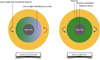 |
Fig. 1 Schematic for the line-of-sight wind maps from Figures 8 and 18. The arrow and disk colors are matched such that the blue arrows paired with green tones indicate flow moving toward the observer, while the red arrows paired with pinkish hues represent the flow moving away. |
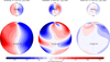 |
Fig. 2 Three-dimensional simulation outputs for three of the eight hot Jupiters in this study. From left to right, the panels showcase (1) a zonal jet-dominated flow, (2) an intermediate transitional regime, and (3) a day-to-night flow pattern. Each column plots the line-of-sight velocity at the P ≈ 0.1 bar atmospheric layer for a single planet. Negative values (blue) denote winds moving toward the observer, while positive values (red) denote winds moving away. The results shown are time-averaged over the last 500 days of their corresponding simulation times. Top: view from the north pole with the SS point and AS point marked. Bottom: view from the dayside. |
2 Methodology
2.1 Choice of planet sequence
For the systematic exploration of the parameter space, we chose targets that are well-observed and are approximately equally spaced in the irradiation flux they receive from their host star. Our sample consists of HD 189733b, WASP-43b, HD 209458b, WASP-31b, WASP-74b, WASP-19b, and WASP-121b. For many of these targets, IR light-curve observations from the Spitzer Space Telescope and Hubble Space Telescope have already been extensively studied and compared to GCM work, including HD 189733b (e.g., Showman et al. 2009; Knutson et al. 2012; Dobbs-Dixon & Agol 2013; Drummond et al. 2018; Steinrueck et al. 2019; Flowers et al. 2019), HD 209458b (e.g., Zellem et al. 2014; Amundsen et al. 2016; Drummond et al. 2018), WASP-43b (e.g., Kataria et al. 2016; Mendonça et al. 2018b; Deitrick et al. 2022), WASP-31b (Kataria et al. 2016), WASP-19b (Wong et al. 2016), and WASP-121b (Parmentier et al. 2018; Lee et al. 2022). Additionally, the planets HD 189733b, WASP-43b, and HD 209458b serve as benchmark objects from the Hubble Space Telescope and Spitzer Space Telescope eras. A comprehensive list of planetary parameters is given in Table 1. For all the presented runs, a 1x solar metallicity was assumed rather than adopted from the referenced papers.
2.2 The dynamical core
In our study, we employ the THOR GCM to simulate atmospheric circulation on exoplanets, as introduced and developed in a series of papers by Mendonça et al. (2016), Mendonça et al. (2018a), Mendonça et al. (2018b), Deitrick et al. (2020), Deitrick et al. (2022), and Noti et al. (2023). THOR is an opensource, fully 3D dynamical core that solves the non-hydrostatic deep (NHD) Euler equations using a horizontally explicit, vertically implicit (Tomita et al. 2002; Wicker & Skamarock 2002) time integrator on an icosahedral grid (Tomita et al. 2001). This split-time integration scheme enables THOR to take a reasonable time step while still maintaining numerical stability with vertically propagating waves in its solutions—waves that would otherwise impose a much smaller time step under the Courant-Friedrichs-Lewy condition. On the other hand, our choice of grid structure overcomes the common limitations of latitude-longitude grids (Staniforth & Thuburn 2012) that suffer from singularities and resolution issues at the poles. This issue extends to all nonuniform grid structures characterized by fixed points with significant variations in cell sizes or crowding. The icosahedral grid, as introduced in Tomita et al. (2001) and Tomita & Satoh (2004), incorporates a quasi-uniform horizontal grid structure. The THOR model uses an altitude grid in the vertical direction and is equipped with two possible configurations. The first setup, as introduced and explained in Mendonça et al. (2016) and Deitrick et al. (2020), utilizes a uniformly spaced altitude grid. The bottom layer altitude is calculated from the ideal gas law, and the top of the atmosphere is a free parameter set by the user. A new option introduced in Noti et al. (2023) allows for finer control of the vertical spacing, incorporating a nonuniform vertical structure. Although the default THOR model primarily solves the NHD Euler equations, as detailed in Deitrick et al. (2020), Deitrick et al. (2022), and Noti et al. (2023), it also offers the flexibility to incorporate various levels of simplification into the governing equations. These include options such as the quasi-hydrostatic deep and the hydrostatic shallow sets of equations, each with their respective assumptions. For this study, our focus remains on the NHD equations, with no simplifying assumptions applied.
All of our newly run models assume solar metallicity and are cloud-free. The comparison cases presented in Section 4 are run with the same setup as presented in Deitrick et al. (2022). All eight of our main model runs were completed with glevel = 5 corresponding to a ≈2° horizontal resolution and 40 vertical layers, uniformly spaced in altitude space with the bottom boundary pressure corresponding to Pref = 1000 bar. The physical height of the uppermost vertical layer varies between models due to their varying sizes and numerical considerations (explained in Section 2.3). This results in a range of pressure levels at the top of the atmosphere, ranging from ≈10−4 bar for our coldest planet in the sample, HD 189733b, to ≈0.05 bar for the hottest planet in our sample, WASP-121b. These values represent the minimum global average pressure, indicating that the entire planet extends to this level in pressure space. However, the actual minimum pressure on the night side reaches ≈10−6 bar across all simulations.
Parameter values assumed for the GCM simulations.
2.3 Stability and numerical parameters
At present, all state-of-the-art GCMs require a numerical dissipation scheme (Jablonowski & Williamson 2011; Heng et al. 2011), representing the dissipation of energy at small, unresolved scales. The simulation domain, especially for giant planets like the ones explored in this study, has characteristic length scales so large that they result in minimum resolved lengths that are still multiple orders of magnitude larger than molecular scales. This limitation usually results in a grid-scale energy build-up. To this end, the THOR model incorporates horizontal and vertical hyperdiffusion terms (Mendonça et al. 2016; Deitrick et al. 2020) and a divergence damping operator. These are, respectively, higher-order gradient terms and a Laplacian that acts on the divergence field. The chosen order of these operators determines which scales the dissipation schemes selectively act on, with higher orders indicating smaller effective scales. Lastly, a sponge layer (Jablonowski & Williamson 2011; Mendonça et al. 2018b) can be introduced upward of a certain altitude to filter out unphysical vertical waves that get reflected from the top of the atmosphere. The sponge layer has the form of a Rayleigh friction term and damps the zonal, meridional, and vertical wind velocities to the zonal averages. All of these additions are modular and can be customized to ensure the stability of a given model run.
Importantly, the choice of dissipation scheme can influence not only the numerical stability but also the emergent large-scale circulation. Recent studies using the “Built on Beowolf” (BOB) (Rivier et al. 2002) model have shown that even brief increases in small-scale energy loss can steer the flow toward markedly different large-scale states (Skinner & Cho 2022, 2025). This indicates that while dissipation schemes are primarily introduced for stability, their design can shape in a nontrivial way the physical interpretation of a simulation. Consequently, models that maintain stability through low spatial resolution, strong explicit viscosity, or basal drag risk suppressing the very small-scale motions that play a key role in shaping global circulation and temperature patterns (Skinner & Cho 2021). Hammond & Abbot (2022) have performed an extensive review of the effect these dissipation schemes have on the THOR GCM, and the reader is advised to consult that work for a comprehensive explanation of these methods.
For the models presented in this work, we utilized all three dissipation schemes. We use 6th-order horizontal and 4th-order vertical hyperdiffusion terms, together with a 6th-order divergence damping operator. Our exact parameters for the numerical setup can be found in Table 2. Our approach mirrors the recent studies done with the THOR GCM (Deitrick et al. 2022; Noti et al. 2023), aiming for comparability.
In addition to the numerical dissipation schemes discussed in this section, many other GCMs utilize an interior boundary drag formulation to account for unmodelled physical processes such as vertical turbulent mixing (Li & Goodman 2010), Lorentz-force braking (Perna et al. 2010), or other processes. THOR does include a Rayleigh drag scheme for the bottom of the simulation domain (Deitrick et al. 2020), but we did not employ it in this work. This option of bottom Rayleigh drag is independent of the top-of-atmosphere sponge layer described above. It is worth emphasizing that we explored simulations with a deep lower boundary (~1000 bar). The atmospheric processes in the upper atmosphere drive these exoplanet atmospheres, and since it would be prohibitively computationally expensive to reach a statistically steady state in the deepest layers due to the very large thermal inertia, we set the lower boundary free of drag, which, in any case, is observationally unconstrained. While there is qualitative motivation for including these dissipation schemes, they are, strictly speaking, unphysical and are not specified from first principles. In other words, they are numerical tools manifesting as additional terms in the Navier-Stokes equation.
Values of hyper-parameters.
2.4 Radiative transfer
The THOR model is equipped with three schemes for the radiative transfer component of our simulations. The model incorporates a two-stream double-gray radiative transfer module, as outlined in Mendonça et al. (2016), Mendonça et al. (2018b), and Deitrick et al. (2020). In addition, we employed a two-stream “picket-fence” non-gray radiative transfer module, as introduced by Noti et al. (2023) and modeled on the approach by Lee et al. (2021). Furthermore, the model includes an “improved two-stream” method for multiwavelength radiative transfer, named Alfrodull (or THOR+HELIOS in Deitrick et al. 2022), that provides an accurate treatment of scattering by medium-sized and large aerosols. This method is originally described in Heng & Kitzmann (2017) and Heng et al. (2018), and involves coupling the THOR GCM with the HELIOS radiative transfer code, as detailed in Deitrick et al. (2022) and referenced in Malik et al. (2017, 2019).
For the main results of this study, we utilized the picket-fence scheme. This decision is grounded in the findings of Noti et al. (2023), who highlighted the picket-fence scheme’s optimal balance between computational efficiency and improved physical accuracy. As discussed in Section 1, our goal is not to conduct a detailed study of each object in our hot Jupiter sample, but rather to perform a parameter-space-wide analysis of dynamical behavior. While the double-gray method provides a simple and fast calculation suitable for parameter-space explorations, the reality of these planets is that gaseous radiative transfer should be nongray (Showman et al. 2020). Although the improved two-stream method would offer a more accurate representation, it requires significantly longer computation times. Thus, the picket-fence scheme offers an excellent trade-off.
The picket-fence method, as described by Chandrasekhar (1935), Parmentier & Guillot (2014), and Parmentier et al. (2015), is a non-gray analytical radiative-transfer approach designed to model the radiative processes of giant planets more accurately than the double-gray approximation. In contrast to the double-gray model, where two constant opacities, k1w and κsw, are used, the picket-fence model employs opacities that are locally interpolated from a pressure-temperature grid. The infrared (IR)opacities are represented by the Rosseland mean opacities, as calculated by Freedman et al. (2014) for a wide range of gaseous giant planets, which we adopted for our study.
The picket-fence model further refines the conventional visual and IR bands used in double-gray approximation by dividing them into five distinct channels: three for the visual band, representing stellar insolation; and two for the IR band, representing planetary emission. This division into multiple channels aims to capture both the continuum opacity and atomic-and molecular line opacities. Using the locally interpolated IR opacities, the opacity structures for the additional IR and visual bands are derived through analytical relationships as detailed in Parmentier & Guillot (2014). For a more comprehensive explanation of the method, we direct the reader to the implementation paper (Noti et al. 2023), which adheres to the conventions established by Lee et al. (2021).
The specific setup for our suite of hot Jupiters assumes solar metallicity for all of our sample planets. We additionally adopt the Rosseland mean opacity tables that include contributions from TiO and VO (as they are presented in Freedman et al. 2014). Since our hot Jupiter sample covers a large range of equilibrium temperatures, including the border region between the hot Jupiter and ultrahot Jupiter classifications, the opacity contributions of these metal oxide species become relevant.
2.5 Characteristic flow quantities
The following sections discuss the flow properties and wave analyses of objects across the parameter space of hot Jupiter dynamics. It is, therefore, important that we introduce commonly defined flow properties (e.g., Showman & Guillot 2002; Perna et al. 2012; Kataria et al. 2016; Showman et al. 2020), proposing them as a natural language through which we can compare our planet sample. To begin with, we calculated the pressure scale height, defined as
 (1)
(1)
where kB (J/K) is the Boltzmann constant, T (K) the temperature of the gas, g (m/s2) the gravity, and m (kg/mol) the molar mass of the gas. Next, we calculated the Rossby number (Holton 1992; Showman & Guillot 2002; Menou et al. 2003), defined as
 (2)
(2)
which quantifies the relative strength of atmospheric dynamics compared to Coriolis effects induced by the planet’s rotation. A Rossby number of order unity indicates a transitional regime where both advection and Coriolis forces are significant, which is crucial for understanding the atmospheric circulation patterns of hot and ultrahot Jupiters. Here, U (m/s) is the characteristic wind speed, L (m) the characteristic length scale, and f = 2Ω sinθ [s−1] the Coriolis parameter with Ω [rad/s] being the rotation rate of the planet and θ [rad] representing the latitude. In our study, we adopted the root mean square (RMS) velocity as the characteristic wind speed. Following the convention of Noti et al. (2023), we adopted the Rossby deformation radius, LD, (Gill 1982; Showman & Guillot 2002), defined as
 (3)
(3)
as the characteristic length scale. This choice is motivated by LD ’s ability to approximate the length scale over which gravity waves and rotational effects balance, thereby providing a meaningful measure for categorizing atmospheric dynamics across our parameter space. Here, N (s−1) is the Brunt-Väisälä frequency and D (m) is the characteristic vertical length scale of a given atmosphere. We chose D = H following our previously mentioned convention. The Rossby deformation radius gives us an approximate length scale over which processes like gravity waves become comparable to rotational effects and is thus a natural choice for the previously defined characteristic horizontal length scale L.
The Brunt-Väisälä frequency, which is a measure of the stability of a stratified fluid to vertical displacements, is defined as (Emanuel 1994)
 (4)
(4)
where θ is the potential temperature. The potential temperature is a measure of the temperature that is corrected for adiabatic expansion. Under the assumption of a constant specific heat capacity cP, which is valid for our GCM runs (see Section 2.7), the potential temperature θ and specific entropy S are related by S = cP ln θ. Consequently, the potential temperature θ, serves as a proxy for entropy, facilitating our analysis of atmospheric stability and dynamics, as further discussed in Section 4.
In this study, we investigate the interplay between stellar irradiation and atmospheric dynamics, focusing on how radiative and dynamical timescales influence atmospheric circulation and wave structures. Specifically, we calculated the associated radiative (trad) and dynamical (tadv) timescales in our simulations (Showman & Guillot 2002):
 (5)
(5)
 (6)
(6)
where Rp is the planetary radius, umax is the maximum zonal wind velocity, cP is the specific heat capacity, σsB is the Stefan-Boltzmann constant, and T is the temperature. These timescales provide us with a simple yet effective way of analyzing the efficiency of heat circulation and the formation of atmospheric wave structures, such as equatorial superrotation. For colder hot Jupiters, (tadv) in the upper atmosphere is shorter or comparable to (trad), allowing dynamical processes to shape the atmospheric flow. Conversely, for hotter objects, the radiative timescale becomes so short that dynamical processes are less effective in forming large-scale structures, particularly in the upper atmosphere.
2.6 Wave analysis
To decompose and analyze wave structures assumed to exist within the highly non-linear solutions produced by a GCM, we required a method well-suited for signals that vary across space (nonstationary) and over time (transient). Some authors have tackled the problem of analyzing wave behavior through Fourier analysis (Mendonça 2020), using a Wheeler & Kiladis (1999)-style analysis (Tan & Showman 2021), or employing a Helmholtz decomposition (Hammond & Lewis 2021; Lewis & Hammond 2022). While Fourier analysis is computationally efficient, easy to understand, and generalizable to multiple dimensions, providing information about the involved spatial scales, it does not offer insights into transient behavior and the time-varying interplay between dynamical structures. Wheeler & Kiladis (1999)-type analyses incorporate a Fourier decomposition of transient structures by averaging out a background assumed to be constant, delivering insights into wave behavior. However, they can be challenging to reproduce exactly due to the variety of possible data preprocessing steps (e.g., the length of the time-averaging window or whether additional filtering techniques are applied), and typically require overlaid theoretical solutions to “guide the eye”. Helmholtz decompositions are adaptable methods that split the field into rotational and divergent components, providing insights into the physical interplay between, for example, Rossby and Kelvin waves. However, they do not offer information regarding the characteristic length and timescales of these waves.
We employ the continuous wavelet transformation (CWT) (Farge 1992) in this work because it allows us to analyze non-stationary and transient structures while providing dominant length and timescales of the physical processes involved from an agnostic perspective without assumptions about the magnitude of these quantities. The only input required is the range of spatial scales over which the data is decomposed; selecting a sufficiently large range effectively mitigates concerns about this parameter. Additionally, wavelet analysis enables us to recover full dispersion relations ω (k), where ω is the temporal frequency of the wave and k is the wave number of the wave. While Wheeler & Kiladis (1999)-style analyses also provide dispersion relations, they cannot simultaneously offer the spatial distribution of decomposition coefficients that help identify which underlying waves are present. Instead, they often overplot theoretical dispersion relations for inertio-gravity, Kelvin, and Rossby waves, which are not fit to the data nor physically justified since they stem from linear analysis.
Wavelet analysis is a time-frequency method that enhances the Fourier transform’s capabilities by capturing both time and frequency (or space and spatial frequency) details from a signal. Using wavelets as decomposition functions distributes the precision of the Fourier transform between time and frequency, allowing analysis of transient structures without the stationarity assumption required by Fourier analysis. However, the information recovered remains constrained by the Heisenberg-Gabor uncertainty1 principle (Morlet et al. 1982), resulting in a natural spread within the derived dispersion relations for wave structures. While optimization techniques (Moca et al. 2021) can reduce this spread, they are beyond the scope of this study.
A simple illustration of the differences between a Fourier decomposition and wavelet decomposition can be found in Figure 3. For illustration purposes, we construct a toy model that consists of an arbitrary series of sinusoidal waves of three different frequencies. The original signal displayed on the top panel consists of three pure sine waves of a given amplitude. The time series evolves as we move from a sine wave with low frequency to sine waves of higher frequencies, and lastly, we combine all three signals. As is evident from the illustration, the Fourier decomposition of such a signal would only be able to tell you that there are three distinct sine waves within this signal. Simply judging from the Fourier transform, we would not be able to differentiate between a sequential version of the same time series, for example, the last part with all three signals combined would have a nearly identical Fourier space representation just by itself. Contrastingly, the bottom panel showing the wavelet decomposition result tells us the time-dependent story of how these simple waves contribute to the overall signal. The above-mentioned spread in the recovered frequency values is also visible.
Before describing our methodology for recovering the wave structures, we would like to define what wavelet functions are and the CWT we use, in addition to our choice of a wavelet function, defining the natural language of this decomposition. A wavelet function describes a short-term oscillation and is defined (Farge 1992) to have zero mean and is confined in both spatial (physical) and frequency (Fourier) domains. We adopt the definition given in Torrence & Compo (1998) and define the CWT as
![Mathematical equation: W_{n}\left(s\right) = \sum_{\tilde{n}=0}^{N-1} x_{\tilde{n}} \Psi^{*} \left[ \frac{\left(\tilde{n} - n\right) \delta t}{s}\right],](/articles/aa/full_html/2025/07/aa53597-24/aa53597-24-eq7.png) (7)
(7)
where xn are the n points in a discrete time series equally spaced out in time by δt, s is the nondimensional wavelet scale that scales the size of that wavelet function, and Ψ* describes the complex conjugate of the wavelet function. The key components of a CWT are the dimensionless scale and time parameters. Given a time-dependent signal, considering the example of the zonal (east-west) component of the GCM velocity field, these parameters stretch the scanning wavelet function and translate it across the dimensionless time axis to calculate the “match” between the zonal wind components and the used wavelet function at a given scale. For our wavelet function, we adopted a Morlet (Morlet et al. 1982) wavelet for the decomposition. The Morlet wavelet function in its general form,
 (8)
(8)
is defined as a plane wave that is modulated by a Gaussian, where η is the dimensionless time parameter and ω0 defines the nondimensional central frequency of the wavelet. Expressed in simple terms, Morlet wavelets are a family of functions describing normalized and decaying local oscillations. Our selection of this wavelet function is grounded in both practical considerations, namely, its successful application in previous atmospheric science studies (Torrence & Compo 1998), and theoretical justification, specifically its capacity to maintain an optimal balance in the time-frequency, or in our case space and spatial frequency, trade-off governed by the Heisenberg-Gabor uncertainty (Morlet et al. 1982). As an extension of the Gabor wavelet (Gabor 1946), the Morlet wavelet was specifically designed to minimize this uncertainty.
We utilize the already existing pyWavelets Python package (Lee et al. 2023) for the wavelet decomposition due to its computational efficiency, together with the fact that their implementation also follows the Torrence & Compo (1998) conventions. As previously mentioned, the only fixed input parameter is a range of spatial scales to decompose our input signal. Following our definitions, these input scales are dimensionless and define how our input wavelet functions will be “stretched”. Given that the sampling period Psampling of the input signal is known, one can relate these dimensionless quantities to their physical values. For recovering spatial frequencies, the sampling period Psampling corresponds to the size of a grid cell. Alternatively, if one is interested in recovering temporal frequencies, this would be the computational time step. To be able to interpret our results in a physically meaningful way, we chose to express our input scales as zonal wave numbers calculated by
 (9)
(9)
where ω0 is the dimensionless central frequency of the wavelet as given in Eq. (8), s the dimensionless scale parameter as given in Eq. (7), and Psampling the above-mentioned sampling period of a given signal. To make the discussion uniform across our hot Jupiter sample, we further adopted the following normalizations
 (10)
(10)
 (11)
(11)
where ωchar is the characteristic temporal frequency, kchar is the characteristic zonal wave number, Rp is the radius, and ωp is the rotation rate of the exoplanet. The choice of the characteristic wave number, kchar, is motivated by the desire to express wave numbers in a dimensionless form that directly relates to a planet’s size. If we consider a wave pattern that completes one full cycle around the planet at the equator, its wavelength must equal the planetary circumference 2πRp. By choosing  , we define a dimensionless wave number, k̂, in which k̂ = 1 represents a wave that fits exactly once around the planet’s circumference. Larger or smaller values of k̂ naturally correspond to waves that repeat multiple times or fractionally around the planet. This normalization thus provides an intuitive measure of how the spatial scales of atmospheric structures relate to the size of the planet itself. Our input wave numbers are identical for all the presented analyses and correspond to the normalized wave-number range k̂ = [0.1,10].
Using the methodology described above, we recover a set of coefficients for the wavelet functions defined for each input scale and for each point in time. In other words, we recover a time-dependent power spectrum of our input zonal wave numbers. As such, we can identify the dominant modes of circulation and recover their dispersion relations ω (k), for a given temporal frequency ω and zonal wave number, k.
To address another important point, we would like to mention how the temporal evolution of the GCM solutions plays a role in our analysis. Conventionally, the GCM results shown in exoplanetary literature are a time average of what would be considered the steady state result after the spin-up period is discarded. This convention relies on the fact that the intention is to study the average global climate state, rather than the temporal evolution of small-scale features. In this sense, the temporal evolution does not portray the true development of how the steady state came into existence. However, in our case, we are interested in the time-dependent production and dissipation of waves, because these are the mechanisms by which the global climate state (i.e., the equatorial jet and the related day-night contrast) is formed, and thus the physical evolution and development of the flow pattern, as the GCM is “spun up” from rest, contains relevant information.
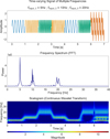 |
Fig. 3 Simple comparison illustrating the differences between a Fourier transform (middle panel) and a CWT (bottom panel). Top: simple timevarying sinusoidal signal composed of successive pure sine waves at different frequencies, culminating in the final second where all three frequencies overlap. Signals of the same frequency have the same color. Middle: fast Fourier transform power spectrum of the signal, providing a single, time-averaged frequency-domain view. Bottom: continuous wavelet transformation scalogram of the same signal, showing how the power at each frequency component changes over time. |
2.7 The transition from hot Jupiters to ultrahot Jupiters
For our fiducial runs, we assumed a standard H2−dominated atmosphere. This choice implies an implicit assumption on the mean molecular weight that modifies the specific heat capacity cp and the specific gas constant Rd. While this assumption proves reasonable for standard hot Jupiter cases, ultrahot Jupiters pose a different challenge. As mentioned in Bell & Cowan (2018) and Tan & Komacek (2019), around the ≈2200-2500 K point for equilibrium temperatures, we move to a different chemical regime, where the molecular hydrogen H2 begins to dissociate from the day side of the atmosphere.
As we probed the lower end of this temperature range with WASP-121b, with an equilibrium temperature of Teq = 2358 K, we attempted to mimic this change in behavior with a simple, idealized case. We assumed χH = 1 and mH ≈ u, resulting in an idealized mean molecular weight μm = 1. This situation corresponds to an atmosphere where hydrogen exists purely in its atomic form. It is important to note that this is different from what was proposed by Bell & Cowan (2018), who suggested that the dayside of an ultrahot Jupiter is dominated by atomic hydrogen, while its nightside is dominated by molecular hydrogen.
As mentioned above, this case is meant to illustrate the upper boundary of the proposed mechanism for modifying the flow. The results are presented in Section 4.
3 Results
3.1 Atmospheric structure of the GCM sequence
To establish the correspondence between previous parametric exploration studies such as Perna et al. (2012), Showman & Polvani (2011), and Noti et al. (2023), together with studies focusing on a sample of observed exoplanets such as Showman et al. (2013) and Kataria et al. (2016), we would like to go over the general circulation properties of our planet sample. As many previous studies have indicated (e.g., Perna et al. 2012; Bell & Cowan 2018; Jones et al. 2022), the relationship between the irradiation temperature and the heat circulation patterns and efficiencies goes through several distinct transitions as we increase or decrease the irradiation temperature.
In Figure 4, we show the upward long-wave radiation flux patterns overlaid with winds at the approximate IR photosphere (P ≈ 0.1 bar). As equilibrium temperatures rise, going from the upper left corner panel to the bottom right corner panel in Figure 4, there is a notable increase in the day-to-night upward long-wave radiation contrast accompanied by a gradual reduction in the eastward hotspot offset. For the colder planets, in the upper row, a distinctive Matsuno-Gill (Matsuno 1966; Gill 1980) chevron pattern emerges. With higher equilibrium temperatures (or increased irradiation temperature), this pattern gradually diminishes, evolving into a singular, prominent hotspot and reinforcing the increasingly pronounced day-night contrast observed in the upward long-wave radiation maps. However, to quantify this contrast more systematically we examined the night-to-day flux ratio. By examining this ratio, we can evaluate how effectively the global circulation transports heat away from the SS point, thereby refining our understanding of the evolving flow patterns suggested by the maps in Figure 4. In Figure 5, we plot the night-to-day upward long-wave radiation flux ratio for each planet and observe a decreasing trend with increasing instellation. This declining ratio serves as a proxy for reduced heat circulation efficiency, confirming that circulation efficiency decreases with higher instellation until the ultrahot Jupiter regime (≈2500 K is reached. Our study only extends until the beginning of the ultrahot Jupiter regime with our mock ultrahot Jupiter example WASP-121b, which shows a marginal increase in the heat circulation efficiency. These results are consistent with previous studies (e.g., Jones et al. 2022; Bell & Cowan 2018) and reproduce the anticipated observational and theoretical behavior. It is important that we again underline the caveat that for the slight increase in our “mock ultrahot Jupiter” case, we focused on changing mean molecular weight without taking into account the subsequent heating and/or cooling; this approach is intended solely as a qualitative reproduction of the expected behavior rather than as an extensive comparison to previous studies.
Figure 6 illustrates the T-P profiles for each planet. The initial profile, which is globally identical, is superimposed with the time-averaged profiles, demonstrating that initial conditions are effectively forgotten. The global T-P structure evolves into a profile that is adiabatic in the interior and nearly isothermal in the upper atmosphere. Significant temperature contrasts arise between the SS and AS points for every planet, growing from a few hundred Kelvin for the coldest planet in the upper-left corner to a couple of thousand Kelvin for the hottest planet in the bottom-right corner. The temperature contrast between the morning and evening terminators also exhibits a distinctive evolution. Initially, the contrast between the terminators narrows (e.g., for HD 209458b, WASP-31b, and WASP-17b), and then it widens again in hotter planets, ultimately stabilizing at a difference of a few hundred Kelvin despite the widening gap between the SS and AS points. We discuss the implications of this shift for the global flow regime in Section 3.2. A thermal inversion layer located between the P ≈ 0.1-1 bar atmospheric layers is evident in most SS point T-P profiles, becoming more pronounced for hotter planets.
Figure 7 shows the zonally averaged zonal winds, revealing an equatorial jet feature in all simulations. As equilibrium temperature increases, the main jet feature at the equator weakens and splits into multiple jets of alternating directions in higher latitudes. In transitioning from HD 189733b (top-left panel) to hotter planets, the originally singular equatorial jet gradually shifts into deeper atmospheric layers. The upper layers, P ≤ 0.1 bar, particularly in the hotter cases shown on the bottom row, exhibit weakening winds. Notably, the peak wind speeds go from ≈2600 m · s−1 for HD 189733b to around 800 m · s−1 for WASP-121b. This phenomenon is further highlighted in Figure 8, which presents a single-layer snapshot of projected line-of-sight velocity viewed from the nightside. The observer’s exact orientation is further detailed in Figure 1. The same dynamics described in Figure 7 appear here: in HD 189733b, the entire evening terminator (spanning P ≈ 10−2 to 10 bar) exhibits negative line-of-sight velocities (i.e., flow toward the observer), while the morning terminator flows away from the observer. Peak velocities concentrate near the equator, consistent with the equatorial jet. As the equilibrium temperature increases from the top-left to the bottom-right panels, the main jet first narrows latitudinally (e.g., in WASP-43b) and later splits into multiple, alternating jets, with the equatorial jet becoming increasingly confined. In the transition from WASP-17b to WASP-121b (bottom row), the equatorial jet remains around P ≈ 1 bar, whereas the upper layers (P ≤ 0.1 bar) develop a growing global SS-to-AS flow. As noted by Showman et al. (2013), an internal return flow, visible in the deeper regions, is required to conserve mass and balance the stronger day-to-night circulation in the upper atmosphere. Although the interior circulation appears weaker, the higher mass flux in these denser layers compensates for that reduced flow.
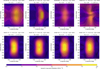 |
Fig. 4 Upward long-wave radiation plots (colored contours) overlaid with the wind field (arrows) at the pressure surface, P = 0.1 bar. Plots are time-averaged over the last 500 days of their corresponding simulation times. |
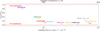 |
Fig. 5 Heat circulation efficiency defined as the ratio of the nightside to dayside upward long-wave radiation fluxes, as a function of the stellar flux received by the hot Jupiter. |
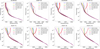 |
Fig. 6 T - P profiles from simulations of the eight hot Jupiters in our GCM sample, including that of the morning terminator, evening terminator, SS point and AS point. Also shown is the globally averaged profile. The initial temperature-pressure profile is shown as a dot-dashed curve. Each curve is accompanied by a shaded region that shows the temporal evolution of each profile, where the first 500 days of spin-up have been excluded. |
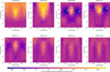 |
Fig. 7 Zonally averaged zonal winds for the eight planets in our GCM sample. Plots are time-averaged over the last 500 days of their corresponding simulation times. |
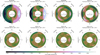 |
Fig. 8 Line-of-sight velocities presented across a slice along the terminator. Equilibrium temperatures increase from the coldest hot Jupiter case in our sample HD 189733b on the upper left corner to the hottest hot Jupiter example in our sample WASP-121b on the bottom right corner. Positive values denote winds moving away from the observer, and the effect of planetary rotation is not taken into account. For guidance in reading this plot, please refer to Figure 1. |
3.2 Global flow transition
In Figure 4, starting from WASP-17b and hotter planets, we observe an equatorial flow opposing the equatorial jet form at the P ≈ 0.1 bar atmospheric layer that is plotted. This feature exists, to a limited extent, even in colder planets such as HD 209458b or WASP-31b, although not as prominently as for the hotter planets. For colder planets, this transition presents itself as the shrinking of the latitudinal extent of the equatorial jet with westward flows forming in the high-latitude regions of their respective atmospheres. As presented in the previous section, the extent and specifics of this dynamical feature can be better observed in Figure 8.
The T-P profiles in Figure 6 highlight the gradual shift in global flow regimes as planetary equilibrium temperatures increase. We can interpret these changes by comparing our physical understanding of two contrasting scenarios: one dominated by an eastward equatorial jet, where heat deposited at the SS point travels eastward to the evening terminator and then around the night side to the morning terminator, and another characterized by day-to-night flow, which heats both terminators more symmetrically despite the underlying eastward mean flow due to the planet’s rotation.
In HD 189733b, the morning terminator is even colder than the AS point, and the evening terminator follows the SS profile, consistent with an eastward superrotating jet distributing heat efficiently. For WASP-43b, the morning terminator and AS temperatures nearly coincide, while the evening terminator, though still above the global mean, is cooler, indicating a weakening of the equatorial jet. In the transitional HD 209458b, the morning terminator now exceeds the AS temperature, and the two terminators have nearly identical profiles. This implies the emergence of day-to-night winds that heat the morning limb, while the diminishing jet is evident from the cooler evening terminator, which lies below the global mean that is skewed toward higher temperatures by an increasingly hotter SS region. For the hottest planets (shown on the bottom row), the temperature difference between the SS and AS regions can exceed 2000 K. Despite this intensified day-to-night gradient, terminator differences stabilize at a few hundred Kelvin, and the evening terminator gradually converges toward the global mean, in line with our expectations of a more symmetric heating for a day-to-night flow.
As day-to-night flow patterns emerge in the hotter planets, we also see a strong connection between these circulation changes and the meridionally averaged potential temperature structure. While potential temperature is typically used to assess atmospheric stability and often plotted in a latitude-pressure framework (e.g., Deitrick et al. 2020), here we examine it against longitude and pressure. This alternative representation not only confirms stable, vertically stratified profiles, but also highlights longitudinal variations that correlate with the evolving circulation regimes. In Figure 9, we recover vertically stratified profiles as expected from convectively stable atmospheres. Beyond this baseline structure, two key findings stand out. First, HD 189733b and WASP-43b show a pronounced longitudinal asymmetry around the SS point at 0°, indicating significantly eastward-shifted hotspots and strong zonal contrasts in potential temperature. Second, all planets feature longitudinal potential temperature gradients, hinting at baroclinic2 instabilities. Since our vertical axis represents constant pressure levels, any horizontal gradient in potential temperature implies a corresponding density gradient, which can drive the instability. In contrast to the colder planets, the hotter planets exhibit more symmetric distributions down to P ≈ 0.5-1 bar. This range corresponds to the vertical depth of their day-to-night flows, as illustrated in Figure 8, which shows the extent of these winds in the upper layers. As equilibrium temperature increases, we observe the hotspot shift diminish and the symmetric region broaden, aligning with the intensified stellar irradiation and the growing dominance of day-to-night circulation.
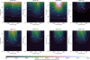 |
Fig. 9 Latitudinally averaged potential temperature plots. The SS point is located at φ = 0. |
3.3 Benchmarking the wavelet analysis method
Having observed the emergence of a general flow transition pattern across our simulated hot Jupiter cases, we would like to understand the atmospheric waves that drive these patterns. For this purpose, we introduced a novel wavelet-based analysis framework in Section 2.6. In order to decode the wave patterns underlying the large-scale flow transitions, we first benchmarked our wavelet analysis method by decomposing time-dependent analytical solutions to the shallow water equations as they are presented in Heng & Workman (2014), but originally derived by Matsuno (1966). These analytical solutions enable us to verify that the method retrieves the correct wave numbers and frequencies, while also exemplifying the kind of output our approach produces. As benchmarks, we used the solutions to the following dispersion relation (equation 106 in Heng & Workman 2014):
 (12)
(12)
where ωR is the real part of the wave frequency, n is the meridional wave number, and k3 is the zonal wave number. This dispersion relation is derived under the equatorial β-plane approximation and the assumption of a balanced, frictionless flow (ωI = 0). The general time-dependent solutions (equation 107 in their work) provide an exact, analytical benchmark for our wavelet analysis method. We adopt the algebraic notation of Heng & Workman (2014), while again noting that these solutions were originally derived by Matsuno (1966) and expanded upon by Gill (1980):
 (13)
(13)
![Mathematical equation: h' = v_{0} ~\exp \left( - \frac {y^{2}}{2} \right) \left( \frac{k}{\omega_{R}} - \frac{\omega_{R}}{k} \right)^{-1} \sin \left( k x - \omega_{R} t \right) \\ \times\left[y \left( \frac{1}{k} + \frac{1}{\omega_{R}}\right) ~\mathcal{H}_{n} - \frac{2n ~\mathcal{H}_{n-1} }{k}\right],](/articles/aa/full_html/2025/07/aa53597-24/aa53597-24-eq15.png) (14)
(14)
![Mathematical equation: v'_{x} = \frac{v_{0}}{k^{2} - \omega_{R}^{2}} ~\exp \left( - \frac{y^{2}}{2} \right) \sin \left( k x - \omega_{R} t \right) \\ \times\left[ y \left( \omega_{R} + k \right) ~\mathcal{H}_{n} - 2n k ~\mathcal{H}_{n-1}\right],](/articles/aa/full_html/2025/07/aa53597-24/aa53597-24-eq16.png) (15)
(15)
where t is time, v0 is an arbitrary normalization constant, ν′x indicates zonal velocity perturbations, h′ refers to shallow water height perturbations, ν′y represents meridional velocity perturbations, and  denotes Hermite polynomials of order n. In the equatorial β-plane approximation, x and y are the horizontal and vertical distances in Cartesian coordinates, which correspond to latitude and longitude on a sphere.
Figure 10 displays a single analytical Rossby wave4 solution to the shallow water equations on the left panel. The right panel of the same figure displays the time-dependent power spectrum of the zonal wind field at y = 0, corresponding to the equator, calculated utilizing the wavelet analysis method. To calculate the zonal wave number, we applied the wavelet decomposition to the zonal velocity perturbations ν′x across x at each y and then repeat it for all y-values. This decomposition identifies a band in wave-number space with oscillating power. The spread of the wave-number band displays the previously mentioned (see Section 2.6) inherent Heisenberg-Gabor uncertainty, which limits the simultaneous precision of the recovered wave numbers and their spatial localization. Analyzing the periodicity of the identified wave number, k, allows us to extract the temporal frequency ωR. Our recovered values for the example, k = 1.038 ± 0.025 and |ωR| = 0.254 ± 0.004, as seen in Figure 10, are consistent with the input values n = 1 and k = 1. Our analysis recovers the absolute value of |ωR| = 0.254, but not its sign, as the wavelet method is unable to extract the travel direction of the wave. While we illustrate results at a single y-location, repeating the same analysis for different y-values or averaging the outcomes over y yields consistent results (not shown). This is an expected outcome given the simplicity of this single-wave example.
When multiple waves with different k values are present, they can partially couple with one another, exacerbating the spread in the multiple identified wave numbers. As an example, illustrated on the left panel of Figure 11, we introduce two Rossby wave solutions with n = [1, 1] and k = [1,3], which correspond to temporal frequencies ωR = - [0.254, 0.251]. As shown on the right panel of Figure 11, our wavelet analysis recovers two distinct wave modes with k = [1.013 ± 0.219, 3.414 ± 0.188] and |ωR| = [0.254 ± 0.005, 0.250 ± 0.004]. These values align closely with the input, despite the expected inherent spread introduced by Heisenberg-Gabor uncertainty and the wave-mode coupling. Overall, these benchmark tests demonstrate that our wavelet method is capable of accurately extracting wave modes from a flow field.
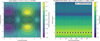 |
Fig. 10 Single analytical wave benchmark example for our wavelet analysis method. Left : Matsuno-Gill type analytical solution that corresponds to a Rossby wave characterized by n = 1; k = 1. Plotted are the zonal wind components overlaid on the shallow water height field. Right: scalogram of the zonal wave number against dimensionless time. Our method correctly identifies the input zonal wave number, k, and the temporal frequency, ωR, consistent within the uncertainties, which is due to the Heisenberg-Gabor uncertainty principle. |
3.4 Applying the wavelet analysis to GCM outputs
In the previous section, we demonstrated our wavelet analysis method by recovering known wave structures from linear shallow-water solutions. This benchmarking served two key purposes: it verified our ability to identify imposed modes (e.g., specific Rossby waves) and introduced the outputs of a wavelet transform, particularly the scalograms5, which show the timeevolving power in different modes. Having established the validity of our approach, we now turn to the more complex, nonlinear flow solutions produced by our GCM.
Unlike the shallow-water test cases, GCM solutions can feature wave interactions that vary significantly with latitude. As also explained in Mendonça (2020), we expected Kelvin waves to dominate near the equator, where they appear as eastwardtraveling features with vanishing meridional components. By contrast, Rossby waves generally vanish near the equator (where the Coriolis force is zero) but emerge at mid- and high latitudes, exhibiting antisymmetric meridional structures. Both wave types are expected to show symmetry about the equator in temperature and zonal wind fields. Consequently, we analyzed the wavelet signals separately at the equator and midlatitudes to capture each wave’s contributions. Beyond the scalograms, we also examined the spatial distributions of the wavelet coefficients. By mapping power in a single wave number across latitude and longitude at a given atmospheric layer, we can confirm if a mode’s structure and symmetry match the expected signatures of Kelvin-Rossby waves. This combined perspective lets us connect each identified mode to a physically interpretable wave structure.
Figures 12 and 13 illustrate this analysis for HD 189733b. In Figure 12, the left panel shows a snapshot of the GCM output at the P ≈ 0.1 bar layer (corresponding to the IR photosphere) at 600 days. The middle and right panels display the scalo-grams at the equator and midlatitudes, respectively, following the approach used in Section 3.3. Figure 13 presents the spatial distribution of wavelet coefficients of the temperature, zonal wind, and meridional wind fields (from left to right) at the same pressure layer for wave numbers, k̂ = 1 and k̂ = 2, averaged over the final 100 days of the 500-day period, thereby providing a link between identified wave modes and physically anticipated wave structures.
Wave numbers, k̂ ≈ 0.3, k̂ ≈ 1, and k̂ = 2, consistently appear in our analyses and form an instructive basis for discussion. By definition (Section 2.6), k̂ = 1 corresponds to a planetary-scale wave; hence, we classify k̂ ≈ 0.7-1.5 as planetary-scale, k̂ ≥ 1.5 as small-scale, and k̂ ≤ 0.7 as large-scale. We decomposed and analyze the simulation output from 100 to 600 days after the start of each run, covering a part of the spin-up phase. The output frequency is set to 0.1 days—less than 25% of the rotation period for all hot Jupiters in our sample (0.81-3.74 days)—to, assuming a Nyquist-like sampling, adequately resolve the oscillations in temperature, zonal wind, and meridional wind. Although applying the same wavelet decomposition at a later time, closer to steady-state, would still identify the waves, omitting the spin-up period would overlook essential details of how they form and interact with the evolving background flow—information that is important for understanding the wave-mean flow interplay that ultimately shapes the global circulation.
For HD 189733b, we observe a well-developed zonal jet in the left panel of Figure 12. The middle panel (the equatorial S scalogram) shows significant power in the planetary-scale k̂ = 1 mode, which diminishes over time and gives way to developing large-scale structures (k̂ ≈ 0.3) around the 350-day mark. A weak contribution from the small-scale k̂ = 2 mode is also visible. The right panel (the midlatitude scalogram) shows a similar pattern: the power initially concentrates in wave numbers, k̂ = 1-2, and, although it fades over time as in the equatorial case, it remains present throughout the analysis period. Meanwhile, a large-scale flow with k̂ ≈ 0.3 emerges. We interpret these large-scale modes as the mean flow modulated by wave-mean flow interactions. The overlap in power near the 170-day mark, coupled with a gradual decrease in planetary- and small-scale power and a corresponding increase in large-scale power, suggests a coupling with the k̂ ≈ 0.3 and k̂ = 1 - 2 modes. This coupling aligns with the onset of equatorial superrotation, seen in the gradual increase in the large-scale mode in the equatorial scalogram.
Inspecting Figure 13 reinforces our interpretation since both wave modes k̂ = 1 and k̂ = 2 display characteristics of coupled Rossby-Kelvin waves: symmetric temperature and zonal-wind structures about the equator, coupled with antisymmetric meridional features at higher latitudes that vanish at the equator. Additionally, the upper middle panel features an equatorial feature reminiscent of the Matsuno-Gill (Matsuno 1966; Gill 1982) chevron pattern. Altogether, these observations paint a picture that is consistent with the Showman & Polvani (2011) explanation of how equatorial superrotation arises. Namely, we expect momentum tobe transported from higher latitudes onto the equator through the coupling of westward-propagating Rossby waves and eastward-propagating equatorial Kelvin waves, creating the characteristic chevron shape.
HD 209458b (Figure 14) exhibits a transitional flow regime. On the left panel, we observe a narrower zonal jet compared to HD 189733b, and mid-to-high-latitude westward flows become more pronounced. The middle panel displays a significant k̂ ≈ 1 mode that persists throughout the analysis period, with slightly increasing power. Meanwhile, a large-scale (k̂ ≈ 0.3) structure develops around the 300-day mark, accompanied by a later weak contribution from smaller scales (k̂ ≈ 3). A similar pattern appears in the right panel, where features of k̂ ≈ 1 and k̂ ≈ 2 persist over the entire analysis period. The k̂ ≈ 1 feature broadens to span k̂ ≈ 0.3-1, peaking near k̂ ≈ 0.5-0.7. The development of this broadening coincides with the emergence of the large-scale feature in the equatorial scalogram, suggesting a coupling of the identified waves similar to what is observed in HD 189733b.
In Figure 15, the k̂ = 1 and k̂ = 2 modes retain Rossby-Kelvin wave characteristics: temperature and zonalwind structures remain symmetric about the equator, while meridional winds are antisymmetric. The meridional wind components still vanish at the equator, displaying the expected Kelvin-wave feature, but this vanishing is confined to within ±10° of the equator, compared with ±30° for HD 189733b in Figure 13. In addition, substantial phase tilts appear at higher latitudes for both the k̂ = 1 and k̂ = 2 modes. The tilted zonal wind features, forming an eastward-pointing chevron shape near the equator, result from the coupling between eastwardpropagating Kelvin waves and westward-propagating Rossby waves. However, in HD 209458b the effect appears weaker than in HD 189733b.
Lastly, WASP-121b (Figure 16) exhibits a fully developed day-to-night flow in the left panel. Both the equatorial and midlatitude scalograms share qualitatively similar patterns, with the strongest signal given by the k̂ - 1 mode. Alongside the planetary-scale wave modes, k̂ ≈ 0.3 and k̂ ≈ 2 are present at both the equator and at midlatitudes, and both modes appear stronger at midlatitudes. The contributions from each wave mode remain steady during the analysis, showing no signs of evolution. At this stage of the simulation, the solutions have not reached a steady-state, and we interpret these modes as the wave response to the instellation and rotation of the planet, which do not display any signs of interactions.
Figure 17 shows that the k̂ = 1 mode lacks strong equatorial signatures. Contributions appear at higher latitudes, where weak Rossby-wave signals persist without coupling to an equatorial Kelvin wave. This pattern aligns with a circulation dominated by direct stellar forcing rather than wave-mean flow interactions. By contrast, the k̂ = 2 panels exhibit some equatorial features, with meridional wind components vanishing only at the equator. This implies that the wave response still gets triggered at smaller scales, but is unable to grow to form planetary-scale dynamical features. The same high-latitude (±60°) phase tilts observed on HD 209458b also occur here. Moreover, the spatial distributions divide into two regions above and below ±60°, coinciding with the temperature feature seen in the upper-left panel, which corresponds to the hotspot. We interpret this boundary as marking the transition from a region with very short radiative timescales that disrupts dynamical formation to the high-latitude zone, where lower temperatures still allow dynamical structures to form.
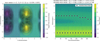 |
Fig. 11 Multi-wave analytical benchmark example for our wavelet analysis method. Left : Matsuno-Gill type analytical solution that corresponds to a combination of Rossby waves characterized by n = 1, 1; k = 1, 3. Plotted are the wind fields overlaid on the shallow water height field. Right: scalogram of the zonal wave number against dimensionless time. Our method correctly identifies the input zonal wave numbers, k, and the temporal frequencies, ωr, within the uncertainties, which is due to the Heisenberg-Gabor uncertainty principle. |
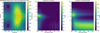 |
Fig. 12 Left panel: snapshot of the GCM solution for HD 189733b at 600 days, showing temperature and wind fields at approximately 0.1 bar. Center and right : wavelet scalograms of the wind field at the equator and midlatitudes, showing prominent k̂ = 1, k̂ = 2, and developing k̂ = 0.3 modes. |
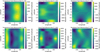 |
Fig. 13 Spatial distribution of wavelet coefficients for the temperature, zonal wind, and meridional wind fields of HD 189733b across the ≈0.1 bar atmospheric layer. The shown results are time-averaged over the last 100 days of the analysis period. Top and bottom panels show the power in modes k̂ = 1 and k̂ = 2, respectively. |
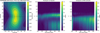 |
Fig. 14 Left panel: snapshot of the GCM solution for HD 209458b at 600 days, showing temperature and wind fields at approximately 0.1 bar. Center and right : wavelet scalograms of the wind field, illustrating a qualitatively similar case to HD 189733b, albeit with a weakening k̂ = 2 contribution. |
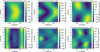 |
Fig. 15 Spatial distribution of wavelet coefficients for the temperature, zonal wind, and meridional wind fields of HD 209458b across the −0.1 bar atmospheric layer. The shown results are time-averaged over the last 100 days of the analysis period. Top and bottom panels show the power in modes k̂ = 1 and k̂ = 2, respectively. |
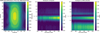 |
Fig. 16 Left panel: snapshot of the GCM solution for WASP-121b at 600 days, showing temperature and wind fields at approximately 0.1 bar. Center and right : scalograms of the zonal wind at the equator and midlatitudes revealing a prominent k̂ ≈ 1 mode in both regions. Large-scale (k̂ ≤ 0.5) and small-scale (k̂ ≥ 1.5) contributions are also evident in both, although they are weaker at the equator. |
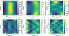 |
Fig. 17 Spatial distribution of wavelet coefficients for the temperature, zonal wind, and meridional wind fields of WASP-121b across the ≈0.1 bar atmospheric layer. The results shown are time-averaged over the last 100 days of the analysis period. Top and bottom panels show the power in modes k̂ = 1 and k̂ = 2, respectively. |
4 Discussion
4.1 Importance of coupling small-scale and large-scale modes
The evolution of the dominant wave-number modes found in Section 3.4 aligns with the theoretical expectations of Showman & Polvani (2011), Showman et al. (2013), and Showman et al. (2020), and the modeling efforts of Mayne et al. (2017). These studies suggest that equatorial superrotation arises from the coupling of smaller-scale eddies to the mean flow, with k̂ ≈ 1 serving as the primary mode for such atmospheres.
As proposed by Mendonça (2020), however, the k̂ = 2 mode also plays a crucial role, representing the smaller-scale eddy features that help drive the equatorial superrotation. Although a one-to-one mapping between wave numbers and physical processes is unfeasible, focusing on the spin-up phase allows us to analyze the atmosphere’s initial response to thermal forcing and planetary rotation, from which we can draw several conclusions. In all of our shown examples in Section 3.4 (Figures 12, 14, and 16), the k̂ = 1 mode consistently appears strongest first as the simulation spins up, followed by the later emergence of the k̂ = 2 and k̂ = 0.3 modes. We propose that the initial emergence of the k̂ = 1 mode reflects a planetary-scale response to thermal forcing. This is supported by the equatorial scalo-grams (Figures 12, 14, and 16), which show slightly stronger k̂ = 1 coefficients than those at midlatitudes, consistent with the equatorial region being hotter and thus exhibiting a stronger response to thermal forcing. Additionally, the steady-state analysis for WASP-121b (Figure A.2) indicates that k̂ = 1 is the only remaining wave mode in the midlatitudes due to intense instellation suppressing dynamic features. Looking at the same figure, we note that for HD 189733b and HD 209458b, where a zonal jet forms, the k̂ = 1 mode is absent or strongly weakened. This observation aligns with our physical expectations since efficient global heat redistribution would inhibit further excitation of the planetary-scale mode. The large-scale mode (k̂ ≈ 0.3) appears to trace both the initial eastward background flow from the planetary rotation and the later developing equatorial superrotation. Additionally, the initial time-dependent behavior offers insight into how these dynamical features interact with each other. The sequence of events suggests that initial instellation-driven thermal forcing sets the stage for wave formation, and only then do the smaller-scale features develop and couple to the main flow.
Our results also show that as equilibrium temperature increases, the contribution of the k̂ = 2 mode weakens. Although this mode remains an important indicator of Rossby and equatorial Kelvin wave activity (i.e., equatorial features with vanishing meridional winds and distinct high-latitude phase tilts), in hotter planets (e.g., WASP-121b) it does not couple effectively with the main flow to drive equatorial superrotation. In other words, while the k̂ = 2 mode in cooler atmospheres can help transport momentum equatorward to drive the formation of the equatorial jet, in hotter planets the incomplete coupling of these small-scale eddies results in the emergence of a dominant day-to-night circulation pattern. This argument is further supported by the fact that the steady-state analysis of HD 189733b (Figure A.2), which shows a persistent k = 2 contribution, suggesting that this mode is responsible for sustaining the existing jet.
We further interpret this shift as reduced circulation efficiency under stronger instellation. When the radiative timescale is shorter than the wave response, small-scale eddies cannot couple effectively with the main flow to sustain dynamical structures. This is evidenced by the zonal phase tilts in WASP-121b (Figure 17), which reveal Rossby-wave features that are not coupled to equatorial Kelvin waves (see Section 3.4). Following the reasoning by Showman & Polvani (2011), such incomplete coupling limits the equatorward transport of angular momentum, resulting in a persistent day-to-night wind pattern that is mainly driven by the thermal forcing of the atmosphere.
4.2 An ultrahot Jupiter case: Modified WASP-121b runs
In previous sections, we focus on how increasing irradiation affects the formation of dynamical features. As our sample transitions toward the ultrahot Jupiter regime, the dissociation of H2 and resulting changes in atmospheric composition are expected to also influence these processes. To explore this, Figure 18 compares our original WASP-121b simulation with a modified “mock ultrahot Jupiter” version. The key difference is in the jet structure: while the original WASP-121b shows multiple alternating jets, the modified version produces a simpler pattern dominated by a strong central jet. This suggests that the modification pushes the circulation profile to resemble those of cooler hot Jupiters, in line with previous findings (Bell & Cowan 2018; Jones et al. 2022).
Physically, this can be understood through the framework proposed by Showman et al. (2013), who argued that shortening radiative timescales can disrupt the formation of the smaller-scale dynamical structures that feed into jet formation. By changing the effective specific heat capacity in our modified simulation to mimic a smaller mean molecular weight, we effectively altered the radiative-dynamic balance. This acts to stabilize dynamical features and makes it appear more zonal-jet-dominated-like. Checking the heat circulation efficiency (Figure 5) confirms that, although we are near the threshold where the trend of increasing irradiation correlating with decreased heat circulation efficiencies may break, our idealized approach of recreating a hot Jupiter-to-ultrahot Jupiter transition improves the circulation efficiency.
Lastly, it is worth noting that the vertical extent of our models does not match perfectly across all simulations (Figure 8), because the lowest pressure attainable on the dayside depends on the instellation. This known limitation of the THOR GCM (Deitrick et al. 2020), shared by other altitude-based GCMs, may slightly alter the upper atmospheric temperature and wind structures. However, this does not fundamentally affect our main conclusions regarding circulation trends and the influence of extreme stellar forcing.
4.3 Opportunities for future work
Our present work aims to analyze parameter space-wide general patterns over a large sample at the cost of decreased complexity. A direct avenue of improvement would be to improve upon our “mock ultrahot Jupiter” case by modeling their atmospheres rigorously and choosing a sample within the hotter ultrahot Jupiter regime to further probe the effects of thermochemical processes on the atmospheres of these gas giant objects. Additional extension possibilities also exist, as there are a myriad of physical processes that could influence the global flow regime transition that we have explored in our work. Some important ones would be to explore the effect of nonsolar metallicities, the effect of chemical kinetics and/or clouds on the presented wave patterns.
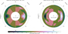 |
Fig. 18 Line-of-sight velocities presented across a slice along the terminator. Positive values denote winds moving away from the observer, and the effect of planetary rotation is not taken into account. For guidance in reading this plot, please refer to Figure 1. Left: unmodified WASP-121b run with mean molecular weight consistent with a molecular hydrogen-dominated atmosphere (μm = 2.35). Right : modified run with mean molecular weight μm = 1. |
5 Conclusion
We confirm the previously reported trend that increasing equilibrium temperatures generally lead to a reduction in atmospheric heat circulation efficiency. Our results also provide evidence for a reversal in this trend, as suggested by Bell & Cowan (2018), around Teq ≈ 2500 K. By artificially altering the mean molecular weight in our WASP-121b simulations, we mimic an upper limit for the expected effects of reaching this ultrahot Jupiter regime and demonstrate a corresponding improvement in circulation efficiency. Additionally, our exploration of transitional flow regimes, as discussed by Showman et al. (2013), suggests that these transitions may extend beyond what was initially proposed. Showman et al. (2013) identified the transition between jet-dominated and day-to-night flow within a three-planet sample (GJ 436b, HD 189733b, and HD 209458b) spanning Teq ≈ 650-1500 K. While we demonstrate the same flow transition as they propose in their work, Showman et al. (2013) present HD 189733b as a transitional case and HD 209458b as an example for a day-to-night-type flow, with any hotter planet falling automatically into this category. In our findings - spanning a range of Teq ≈ 1100-2400 K - HD 189733b and WASP-43b show zonal-jet-dominated flows; HD 209458b, WASP-31b, and WASP-17b occupy a transitional regime; and WASP-74b, WASP-19b, and WASP-121b exhibit day-to-night flow. It is worth noting that, while our findings are also model-dependent and inexhaustive, they suggest that the flow regime transition is not a sharp cutoff at HD 209458b. Rather, it depends on multiple factors, such as the atmospheric composition, as demonstrated in our idealized case, and is better characterized by the coupling or decoupling of underlying wave structures.
We approached this problem by applying our novel waveanalysis method to a sample of eight planets spanning from warm Jupiters to an ultrahot Jupiter-like regime. We identify a shift in the relative importance of smaller-scale eddy modes and their coupling to the mean flow. At lower equilibrium temperatures, both k̂ = 1 and k̂ = 2 modes contribute to sustaining equatorial superrotation. However, at higher irradiation levels, the k̂ = 2 mode weakens, leaving a predominantly planetary-scale circulation. This change corresponds to a regime where day-tonight winds dominate, diminishing the dynamical influence of smaller-scale features.
Our results support the theoretical frameworks put forth by Showman & Polvani (2011) and Showman et al. (2013), as well as the analysis performed by Mendonça (2020) by explicitly identifying the interaction between Rossby and Kelvin waves. Taken together, the extent of our parameter space demonstrates that the key dynamical turning point is the progressive decoupling of the small-scale k̂ ≈ 2 modes from the dominant planetary-scale k̂ = 1 mode.
Overall, these findings refine our understanding of how atmospheric circulation patterns evolve with increasing stellar insolation and provide a more comprehensive framework for interpreting the dynamical behavior of hot and ultrahot Jupiter atmospheres. They also highlight the importance of capturing the interplay between large-scale modes and smaller-scale eddies and point the way toward more sophisticated modeling efforts. This work can help guide future observations and modeling studies aimed at better understanding these extreme atmospheric regimes.
Appendix A Additional wave analysis results
A.1 Large-scale wave modes
In Figure A.1, we show the spatial distribution of the wavelet coefficients for the temperature, zonal wind, and meridional wind fields on the ≈0.1 bar atmospheric layer for HD 189733b,HD 209458b, and WASP-121b. We focus on modes k̂ = 0.3 as a proxy for the large-scale features discussed in Section 3.4.
For HD 189733b (Figure A.1a), a dominant equatorial structure in the zonal wind field appears along all longitudes, representing the zonal-jet-dominated mean flow. In HD 209458b (Figure A.1b), the large-scale equatorial mean flow is also present, and we begin to see symmetrical contributions from the midlatitude regions. By contrast, WASP-121b (Figure A.1c) does not display a robust equatorial zonal wind feature and instead exhibits more symmetric structures in the midlatitudes. An additional effect that is present in all of these plots is that the wavelet coefficients appear to be organized in vertical bands, looking as if the underlying field has not been sampled on a fine enough grid. What we observe here is again the Heisenberg-Gabor uncertainty, which becomes more pronounced for lower wave numbers, k̂, i.e., larger scales.
A.2 Wavelet analysis of steady-state solutions
For completeness, Figure A.2 shows scalograms for the final 500 days of the total simulation time in our example cases. Focusing on HD 189733b, on the left panel, the equatorial superrotation feature has gotten broader in latitude and is the only clear dynamical feature. The hotspot offset is also more pronounced than in Figure 12. Both the equatorial and midlatitude scalo-grams look nearly identical, featuring a broad, large-scale mode (k̂ ≈ 0.2-0.3) and a smaller-scale mode (k̂ ≈ 2). This observation aligns with physical expectations, as the large-scale mode corresponds to the steady-state zonal jet. The similarity between the equatorial and midlatitude scalograms indicates that the dynamical features are strongly coupled in both regions. Furthermore, the k̂ = 2 mode persists as a response continuously triggered by stellar irradiation and planetary rotation, transferring momentum up-gradient. Both modes’ temporal frequencies have lengthened enough to appear nearly constant, supporting our interpretation that this represents a steady-state standing wave.
HD 209458b represents our transitional case. From the middle-left panel, it is evident that it closely resembles its early stages presented in 14. The equatorial jet feature is less pronounced and slightly narrower, mid- and high-latitude westward flows remain, and the hotspot is less prominent, indicating that heat has been transported to some extent around the planet. The scalograms are qualitatively very similar to those of the HD 189733b case. Again, we observe a large-scale mode (k̂ ≈ 0.2-0.3) and a smaller-scale mode (k = 1.5-2). In addition, there seems to be a weak contribution from a planetary-scale wave mode at k ≈ 0.8. While all inspected wave modes remain constant in power throughout the analysis period, apart from intermittent spikes in power in the small-scale mode, suggesting a steady state, these modes appear to oscillate with a high temporal frequency, in contrast to the HD 189733b case. This implies that, although the circulation is still dynamically efficient enough to form the large-scale superrotating feature, the increased instel-lation disrupts its progression into a fully zonal-jet-dominated regime.
WASP-121b is the hottest planet in our sample and represents our day-to-night flow case. Although the left panel shows a flow regime that is similar to what is shown in Figure 16, the scalograms present a significantly different picture. At the equator, two very broad signals span almost the entire wave-number range: one at k̂ = 0.1 - 0.8 and another centered around k̂ ≈ 1.5, with intermittent spikes extending to k̂ ≈ 4 - 5. Combining this observation with the snapshot on the left panel, we conclude that no dynamical wave features can form apart from the day-to-night flow, which arises due to the thermal gradient between the day-and nightsides. The existence of these small-scale features hints that wave responses do get excited in the GCM solutions but do not couple to the main flow, as the short radiative timescales in this region disrupt the formation of any dynamical structures. At midlatitudes, we identify two wave modes: one planetary-scale mode with k̂ ≈ 1 and one small-scale mode with k̂ ≈ 2. Although no large-scale feature is identified, the presence of these modes suggests that the midlatitude region may be cool enough, i.e., the radiative timescale is sufficiently long, for some dynamical structures to form.
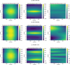 |
Fig. A.1 Spatial distribution of wavelet coefficients of the large-scale mode k̂ = 0.3 at the 0.1 bar atmospheric layer. The results shown are time-averaged over the last 100 days of the analysis period. |
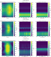 |
Fig. A.2 Left panel: Snapshot of the GCM solutions for HD 189733b, HD 209458b, and WASP-121b at 300 days after the full simulation time (≈4000-5000 days), showing temperature and wind fields at the approximate 0.1 bar atmospheric layer. Center & Right: Wavelet scalograms of the zonal wind field at the equator and midlatitudes, respectively. |
References
- Amundsen, D. S., Mayne, N. J., Baraffe, I., et al. 2016, A&A, 595, A36 [NASA ADS] [CrossRef] [EDP Sciences] [Google Scholar]
- Anderson, D. R., Collier Cameron, A., Gillon, M., et al. 2011, A&A, 528, A97 [Google Scholar]
- Arcangeli, J., Désert, J.-M., Line, M. R., et al. 2018, ApJ, 855, L30 [Google Scholar]
- Bell, T. J., & Cowan, N. B. 2018, ApJ, 857, L20 [Google Scholar]
- Boyajian, T. S., von Braun, K., Feiden, G. A., et al. 2015, ApJ, 800, 51 [Google Scholar]
- Cartes, Z. E., Zuleta, J., López, R., & Rojo, P. 2020, A&A, 642, A29 [NASA ADS] [CrossRef] [EDP Sciences] [Google Scholar]
- Chandrasekhar, S. 1935, MNRAS, 96, 21 [NASA ADS] [Google Scholar]
- Cooper, C. S., & Showman, A. P. 2005, ApJ, 629, L45 [NASA ADS] [CrossRef] [Google Scholar]
- Daubechies, I., & Bates, B. J. 1993, Acoust. Soc. Am. J., 93, 1671 [Google Scholar]
- Dawson, R. I., & Johnson, J. A. 2018, ARA&A, 56, 175 [Google Scholar]
- Deitrick, R., Mendonça, J. M., Schroffenegger, U., et al. 2020, ApJS, 248, 30 [NASA ADS] [CrossRef] [Google Scholar]
- Deitrick, R., Heng, K., Schroffenegger, U., et al. 2022, MNRAS, 512, 3759 [NASA ADS] [CrossRef] [Google Scholar]
- Delrez, L., Santerne, A., Almenara, J. M., et al. 2016, MNRAS, 458, 4025 [NASA ADS] [CrossRef] [Google Scholar]
- Dobbs-Dixon, I., & Agol, E. 2013, MNRAS, 435, 3159 [NASA ADS] [CrossRef] [Google Scholar]
- Drummond, B., Mayne, N. J., Manners, J., et al. 2018, ApJ, 869, 28 [NASA ADS] [CrossRef] [Google Scholar]
- Emanuel, K. 1994, Atmospheric Convection (Oxford University Press) [CrossRef] [Google Scholar]
- Farge, M. 1992, Annu. Rev. Fluid Mech., 24, 395 [Google Scholar]
- Flowers, E., Brogi, M., Rauscher, E., Kempton, E. M. R., & Chiavassa, A. 2019, AJ, 157, 209 [Google Scholar]
- Freedman, R. S., Lustig-Yaeger, J., Fortney, J. J., et al. 2014, ApJS, 214, 25 [CrossRef] [Google Scholar]
- Gabor, D. 1946, J. Inst. Electr. Eng. Part III: Radio Commun. Eng., 93, 445 [Google Scholar]
- Gill, A. E. 1980, Q. J. Roy. Meteorol. Soc., 106, 447 [Google Scholar]
- Gill, A. 1982, Atmosphere-Ocean Dynamics, Atmosphere-Ocean Dynamics, 30 (Elsevier Science) [Google Scholar]
- Guillot, T., Burrows, A., Hubbard, W. B., Lunine, J. I., & Saumon, D. 1996, ApJ, 459, L35 [Google Scholar]
- Hammond, M., & Abbot, D. S. 2022, MNRAS, 511, 2313 [NASA ADS] [CrossRef] [Google Scholar]
- Hammond, M., & Lewis, N. T. 2021, PNAS, 118, e2022705118 [NASA ADS] [CrossRef] [Google Scholar]
- Hellier, C., Anderson, D. R., Collier Cameron, A., et al. 2011, A&A, 534, A20 [Google Scholar]
- Heng, K., & Kitzmann, D. 2017, ApJS, 232, 20 [Google Scholar]
- Heng, K., & Showman, A. P. 2015, Annu. Rev. Earth Planet. Sci., 43, 509 [CrossRef] [Google Scholar]
- Heng, K., & Workman, J. 2014, ApJS, 213, 27 [CrossRef] [Google Scholar]
- Heng, K., Menou, K., & Phillipps, P. J. 2011, MNRAS, 413, 2380 [NASA ADS] [CrossRef] [Google Scholar]
- Heng, K., Malik, M., & Kitzmann, D. 2018, ApJS, 237, 29 [CrossRef] [Google Scholar]
- Holton, J. R. 1992, An introduction to dynamic meteorology, International geophysics series (San Diego, New York: Academic Press) [Google Scholar]
- Jablonowski, C., & Williamson, D. L. 2011, in Numerical Techniques for Global Atmospheric Models, eds. P. H. Lauritzen, C. Jablonowski, M. A. Taylor, & R. Ramachandran (Berlin: Springer), 381 [Google Scholar]
- Jones, K., Morris, B. M., Demory, B. O., et al. 2022, A&A, 666, A118 [NASA ADS] [CrossRef] [EDP Sciences] [Google Scholar]
- Kataria, T., Sing, D. K., Lewis, N. K., et al. 2016, ApJ, 821, 9 [NASA ADS] [CrossRef] [Google Scholar]
- Knutson, H. A., Lewis, N., Fortney, J. J., et al. 2012, ApJ, 754, 22 [NASA ADS] [CrossRef] [Google Scholar]
- Komacek, T. D., & Showman, A. P. 2016, ApJ, 821, 16 [CrossRef] [Google Scholar]
- Lee, E. K. H., Parmentier, V., Hammond, M., et al. 2021, MNRAS, 506, 2695 [NASA ADS] [CrossRef] [Google Scholar]
- Lee, E. K. H., Prinoth, B., Kitzmann, D., et al. 2022, MNRAS, 517, 240 [NASA ADS] [CrossRef] [Google Scholar]
- Lee, G., Gommers, R., Wohlfahrt, K., et al. 2023, https://doi.org/10.5281/zenodo.10152272 [Google Scholar]
- Lewis, N. T., & Hammond, M. 2022, ApJ, 941, 171 [NASA ADS] [CrossRef] [Google Scholar]
- Li, J., & Goodman, J. 2010, ApJ, 725, 1146 [NASA ADS] [CrossRef] [Google Scholar]
- Malik, M., Grosheintz, L., Mendonça, J. M., et al. 2017, AJ, 153, 56 [Google Scholar]
- Malik, M., Kitzmann, D., Mendonça, J. M., et al. 2019, AJ, 157, 170 [Google Scholar]
- Matsuno, T. 1966, J. Meteorol. Soc. Japan, 44, 25 [Google Scholar]
- Mayne, N. J., Debras, F., Baraffe, I., et al. 2017, A&A, 604, A79 [NASA ADS] [CrossRef] [EDP Sciences] [Google Scholar]
- Mendonça, J. M. 2020, MNRAS, 491, 1456 [CrossRef] [Google Scholar]
- Mendonça, J. M., Grimm, S. L., Grosheintz, L., & Heng, K. 2016, ApJ, 829, 115 [CrossRef] [Google Scholar]
- Mendonça, J. M., Malik, M., Demory, B.-O., & Heng, K. 2018a, AJ, 155, 150 [Google Scholar]
- Mendonça, J. M., Tsai, S.-m., Malik, M., Grimm, S. L., & Heng, K. 2018b, ApJ, 869, 107 [CrossRef] [Google Scholar]
- Menou, K., Cho, J. Y. K., Seager, S., & Hansen, B. M. S. 2003, ApJ, 587, L113 [NASA ADS] [CrossRef] [Google Scholar]
- Moca, V. V., Bârzan, H., Nagy-Dabâcan, A., & Muresan, R. C. 2021, Nat. Commun., 12, 337 [Google Scholar]
- Morlet, J., Arens, G., Fourgeau, E., & Giard, D. 1982, Geophysics, 47, 222 [NASA ADS] [CrossRef] [Google Scholar]
- Noti, P. A., Lee, E. K. H., Deitrick, R., & Hammond, M. 2023, MNRAS, 524, 3396 [NASA ADS] [CrossRef] [Google Scholar]
- Parmentier, V., & Guillot, T. 2014, A&A, 562, A133 [NASA ADS] [CrossRef] [EDP Sciences] [Google Scholar]
- Parmentier, V., Guillot, T., Fortney, J. J., & Marley, M. S. 2015, A&A, 574, A35 [NASA ADS] [CrossRef] [EDP Sciences] [Google Scholar]
- Parmentier, V., Line, M. R., Bean, J. L., et al. 2018, A&A, 617, A110 [NASA ADS] [CrossRef] [EDP Sciences] [Google Scholar]
- Perez-Becker, D., & Showman, A. P. 2013, ApJ, 776, 134 [NASA ADS] [CrossRef] [Google Scholar]
- Perna, R., Menou, K., & Rauscher, E. 2010, ApJ, 719, 1421 [NASA ADS] [CrossRef] [Google Scholar]
- Perna, R., Heng, K., & Pont, F. 2012, ApJ, 751, 59 [NASA ADS] [CrossRef] [Google Scholar]
- Rivier, L., Loft, R., & Polvani, L. M. 2002, Monthly Weather Rev., 130, 1384 [Google Scholar]
- Showman, A. P., & Guillot, T. 2002, A&A, 385, 166 [NASA ADS] [CrossRef] [EDP Sciences] [Google Scholar]
- Showman, A. P., & Polvani, L. M. 2011, ApJ, 738, 71 [Google Scholar]
- Showman, A. P., Fortney, J. J., Lian, Y., et al. 2009, ApJ, 699, 564 [NASA ADS] [CrossRef] [Google Scholar]
- Showman, A. P., Fortney, J. J., Lewis, N. K., & Shabram, M. 2013, ApJ, 762, 24 [Google Scholar]
- Showman, A. P., Lewis, N. K., & Fortney, J. J. 2015, ApJ, 801, 95 [NASA ADS] [CrossRef] [Google Scholar]
- Showman, A. P., Tan, X., & Parmentier, V. 2020, Space Sci. Rev., 216, 139 [Google Scholar]
- Skinner, J. W., & Cho, J. Y. K. 2021, MNRAS, 504, 5172 [NASA ADS] [CrossRef] [Google Scholar]
- Skinner, J. W., & Cho, J. Y. K. 2022, MNRAS, 511, 3584 [NASA ADS] [CrossRef] [Google Scholar]
- Skinner, J. W., & Cho, J. Y. K. 2025, ApJ, 982, 64 [Google Scholar]
- Staniforth, A., & Thuburn, J. 2012, Q. J. Roy. Meteorol. Soc., 138, 1 [Google Scholar]
- Stassun, K. G., Corsaro, E., Pepper, J. A., & Gaudi, B. S. 2017, AJ, 153, 136 [NASA ADS] [CrossRef] [Google Scholar]
- Steinrueck, M. E., Parmentier, V., Showman, A. P., Lothringer, J. D., & Lupu, R. E. 2019, ApJ, 880, 14 [Google Scholar]
- Tan, X., & Komacek, T. D. 2019, ApJ, 886, 26 [Google Scholar]
- Tan, X., & Showman, A. P. 2021, MNRAS, 502, 2198 [NASA ADS] [CrossRef] [Google Scholar]
- Tomita, H., & Satoh, M. 2004, Fluid Dyn. Res., 34, 357 [NASA ADS] [CrossRef] [Google Scholar]
- Tomita, H., Tsugawa, M., Satoh, M., & Goto, K. 2001, J. Computat. Phys., 174, 579 [Google Scholar]
- Tomita, H., Satoh, M., & Goto, K. 2002, J. Computat. Phys., 183, 307 [Google Scholar]
- Torrence, C., & Compo, G. P. 1998, Bull. Am. Meteorol. Soc., 79, 61 [Google Scholar]
- Torres, G., Winn, J. N., & Holman, M. J. 2008, ApJ, 677, 1324 [Google Scholar]
- Tsai, S.-M., Dobbs-Dixon, I., & Gu, P.-G. 2014, ApJ, 793, 141 [NASA ADS] [CrossRef] [Google Scholar]
- Wheeler, M., & Kiladis, G. N. 1999, J. Atmos. Sci., 56, 374 [CrossRef] [Google Scholar]
- Wicker, L. J., & Skamarock, W. C. 2002, Monthly Weather Rev., 130, 2088 [Google Scholar]
- Wong, I., Knutson, H. A., Kataria, T., et al. 2016, ApJ, 823, 122 [NASA ADS] [CrossRef] [Google Scholar]
- Zellem, R., Griffith, C. A., Lewis, N. K., Swain, M. R., & Knutson, H. A. 2014, in AAS/Division for Planetary Sciences Meeting Abstracts, 46, 104.04 [NASA ADS] [Google Scholar]
Also known as the Gabor limit (Gabor 1946), after Dennis Gabor, this notion extends Heisenberg’s relation to signal analysis; in essence, a function and its Fourier transform cannot both be strictly bounded.
We use the term “baroclinic” more generally: any misalignment between pressure surfaces and density surfaces represents a source of potential energy that can drive large-scale flow instabilities. On Earth that misalignment primarily results from equator-to-pole temperature contrasts; on other planets, or in particular dynamical regimes, significant day-night gradients can play the same role.
In the current and following equations, adopted from Heng & Workman (2014), we denote the zonal wave number as k, which corresponds to kx in their work.
For clarification, the Rossby waves referenced in the main text refer to Rossby-type solutions to the shallow water equations under the equatorial β-plane approximation, as described in Matsuno (1966).
Scalograms are time-dependent power spectra produced by a wavelet transform. For an introduction to wavelet transform terminology and applications, see Daubechies & Bates (1993).
All Tables
All Figures
|
Fig. 1 Schematic for the line-of-sight wind maps from Figures 8 and 18. The arrow and disk colors are matched such that the blue arrows paired with green tones indicate flow moving toward the observer, while the red arrows paired with pinkish hues represent the flow moving away. |
| In the text | |
|
Fig. 2 Three-dimensional simulation outputs for three of the eight hot Jupiters in this study. From left to right, the panels showcase (1) a zonal jet-dominated flow, (2) an intermediate transitional regime, and (3) a day-to-night flow pattern. Each column plots the line-of-sight velocity at the P ≈ 0.1 bar atmospheric layer for a single planet. Negative values (blue) denote winds moving toward the observer, while positive values (red) denote winds moving away. The results shown are time-averaged over the last 500 days of their corresponding simulation times. Top: view from the north pole with the SS point and AS point marked. Bottom: view from the dayside. |
| In the text | |
|
Fig. 3 Simple comparison illustrating the differences between a Fourier transform (middle panel) and a CWT (bottom panel). Top: simple timevarying sinusoidal signal composed of successive pure sine waves at different frequencies, culminating in the final second where all three frequencies overlap. Signals of the same frequency have the same color. Middle: fast Fourier transform power spectrum of the signal, providing a single, time-averaged frequency-domain view. Bottom: continuous wavelet transformation scalogram of the same signal, showing how the power at each frequency component changes over time. |
| In the text | |
|
Fig. 4 Upward long-wave radiation plots (colored contours) overlaid with the wind field (arrows) at the pressure surface, P = 0.1 bar. Plots are time-averaged over the last 500 days of their corresponding simulation times. |
| In the text | |
|
Fig. 5 Heat circulation efficiency defined as the ratio of the nightside to dayside upward long-wave radiation fluxes, as a function of the stellar flux received by the hot Jupiter. |
| In the text | |
|
Fig. 6 T - P profiles from simulations of the eight hot Jupiters in our GCM sample, including that of the morning terminator, evening terminator, SS point and AS point. Also shown is the globally averaged profile. The initial temperature-pressure profile is shown as a dot-dashed curve. Each curve is accompanied by a shaded region that shows the temporal evolution of each profile, where the first 500 days of spin-up have been excluded. |
| In the text | |
|
Fig. 7 Zonally averaged zonal winds for the eight planets in our GCM sample. Plots are time-averaged over the last 500 days of their corresponding simulation times. |
| In the text | |
|
Fig. 8 Line-of-sight velocities presented across a slice along the terminator. Equilibrium temperatures increase from the coldest hot Jupiter case in our sample HD 189733b on the upper left corner to the hottest hot Jupiter example in our sample WASP-121b on the bottom right corner. Positive values denote winds moving away from the observer, and the effect of planetary rotation is not taken into account. For guidance in reading this plot, please refer to Figure 1. |
| In the text | |
|
Fig. 9 Latitudinally averaged potential temperature plots. The SS point is located at φ = 0. |
| In the text | |
|
Fig. 10 Single analytical wave benchmark example for our wavelet analysis method. Left : Matsuno-Gill type analytical solution that corresponds to a Rossby wave characterized by n = 1; k = 1. Plotted are the zonal wind components overlaid on the shallow water height field. Right: scalogram of the zonal wave number against dimensionless time. Our method correctly identifies the input zonal wave number, k, and the temporal frequency, ωR, consistent within the uncertainties, which is due to the Heisenberg-Gabor uncertainty principle. |
| In the text | |
|
Fig. 11 Multi-wave analytical benchmark example for our wavelet analysis method. Left : Matsuno-Gill type analytical solution that corresponds to a combination of Rossby waves characterized by n = 1, 1; k = 1, 3. Plotted are the wind fields overlaid on the shallow water height field. Right: scalogram of the zonal wave number against dimensionless time. Our method correctly identifies the input zonal wave numbers, k, and the temporal frequencies, ωr, within the uncertainties, which is due to the Heisenberg-Gabor uncertainty principle. |
| In the text | |
|
Fig. 12 Left panel: snapshot of the GCM solution for HD 189733b at 600 days, showing temperature and wind fields at approximately 0.1 bar. Center and right : wavelet scalograms of the wind field at the equator and midlatitudes, showing prominent k̂ = 1, k̂ = 2, and developing k̂ = 0.3 modes. |
| In the text | |
|
Fig. 13 Spatial distribution of wavelet coefficients for the temperature, zonal wind, and meridional wind fields of HD 189733b across the ≈0.1 bar atmospheric layer. The shown results are time-averaged over the last 100 days of the analysis period. Top and bottom panels show the power in modes k̂ = 1 and k̂ = 2, respectively. |
| In the text | |
|
Fig. 14 Left panel: snapshot of the GCM solution for HD 209458b at 600 days, showing temperature and wind fields at approximately 0.1 bar. Center and right : wavelet scalograms of the wind field, illustrating a qualitatively similar case to HD 189733b, albeit with a weakening k̂ = 2 contribution. |
| In the text | |
|
Fig. 15 Spatial distribution of wavelet coefficients for the temperature, zonal wind, and meridional wind fields of HD 209458b across the −0.1 bar atmospheric layer. The shown results are time-averaged over the last 100 days of the analysis period. Top and bottom panels show the power in modes k̂ = 1 and k̂ = 2, respectively. |
| In the text | |
|
Fig. 16 Left panel: snapshot of the GCM solution for WASP-121b at 600 days, showing temperature and wind fields at approximately 0.1 bar. Center and right : scalograms of the zonal wind at the equator and midlatitudes revealing a prominent k̂ ≈ 1 mode in both regions. Large-scale (k̂ ≤ 0.5) and small-scale (k̂ ≥ 1.5) contributions are also evident in both, although they are weaker at the equator. |
| In the text | |
|
Fig. 17 Spatial distribution of wavelet coefficients for the temperature, zonal wind, and meridional wind fields of WASP-121b across the ≈0.1 bar atmospheric layer. The results shown are time-averaged over the last 100 days of the analysis period. Top and bottom panels show the power in modes k̂ = 1 and k̂ = 2, respectively. |
| In the text | |
|
Fig. 18 Line-of-sight velocities presented across a slice along the terminator. Positive values denote winds moving away from the observer, and the effect of planetary rotation is not taken into account. For guidance in reading this plot, please refer to Figure 1. Left: unmodified WASP-121b run with mean molecular weight consistent with a molecular hydrogen-dominated atmosphere (μm = 2.35). Right : modified run with mean molecular weight μm = 1. |
| In the text | |
|
Fig. A.1 Spatial distribution of wavelet coefficients of the large-scale mode k̂ = 0.3 at the 0.1 bar atmospheric layer. The results shown are time-averaged over the last 100 days of the analysis period. |
| In the text | |
|
Fig. A.2 Left panel: Snapshot of the GCM solutions for HD 189733b, HD 209458b, and WASP-121b at 300 days after the full simulation time (≈4000-5000 days), showing temperature and wind fields at the approximate 0.1 bar atmospheric layer. Center & Right: Wavelet scalograms of the zonal wind field at the equator and midlatitudes, respectively. |
| In the text | |
Current usage metrics show cumulative count of Article Views (full-text article views including HTML views, PDF and ePub downloads, according to the available data) and Abstracts Views on Vision4Press platform.
Data correspond to usage on the plateform after 2015. The current usage metrics is available 48-96 hours after online publication and is updated daily on week days.
Initial download of the metrics may take a while.