| Issue |
A&A
Volume 699, July 2025
|
|
|---|---|---|
| Article Number | A156 | |
| Number of page(s) | 14 | |
| Section | Celestial mechanics and astrometry | |
| DOI | https://doi.org/10.1051/0004-6361/202453525 | |
| Published online | 04 July 2025 | |
Astrometry-only detection of microlensing events with Gaia
1
Institute of Physics of the Czech Academy of Sciences,
Na Slovance 1999/2,182 21 Praha 8,
Prague,
Czech Republic
2
Center for Astrophysics and Cosmology, University of Nova Gorica,
Vipavska 11c,
5270
Ajdovščina,
Slovenia
3
Astronomical Observatory, University of Warsaw,
Al. Ujazdowskie 4,
00-478
Warszawa,
Poland
4
Aalta Lab d.o.o.,
Soška cesta 17,
5250
Solkan,
Slovenia
5
Astronomical Observatory,
Volgina 7,
11000
Belgrade,
Serbia
6
Argelander-Institut für Astronomie, Universität Bonn,
Auf dem Hügel 71,
53121
Bonn,
Germany
7
Research School of Astronomy and Astrophysics, Australian National University,
Mount Stromlo Observatory, Cotter Road Weston Creek,
ACT 2611,
Australia
8
Zentrum für Astronomie der Universität Heidelberg, Astronomisches Rechen-Institut,
Mönchhofstr. 12-14,
69120
Heidelberg,
Germany
★ Corresponding author: jankovic@fzu.cz
Received:
19
December
2024
Accepted:
24
May
2025
Context. Astrometric microlensing events occur when a massive object passes between a distant source and the observer, causing a shift of the light centroid. The precise astrometric measurements of the Gaia mission provide an unprecedented opportunity to detect and analyse these events, revealing properties of lensing objects such as their mass and distance.
Aims. We developed and tested the Gaia Astrometric Microlensing Events (GAME) Filter, a software tool for identifying astrometric microlensing events and deriving lensing object properties.
Methods. We generated mock Gaia observations for different magnitudes, different numbers of Gaia visits, and events extending beyond Gaia’s observational run. We applied GAME Filter to these datasets and validated its performance. We also assessed the rate of false positives involving binary astrometric systems misidentified as microlensing events.
Results. GAME Filter successfully recovers microlensing parameters for strong events. Parameters are more difficult to recover for short events and those extending beyond Gaia’s run, where only a fraction of the events are observed. The astrometric effect breaks the degeneracy in the microlensing parallax present in photometric microlensing. For fainter sources, the observed signal weakens, reducing recovered events and increasing parameter errors. However, even for Gaia G-band magnitude 19, the parameters can be recovered for Einstein radii ≳2 mas. Observing regions with varying numbers of Gaia visits has a minimal impact on filter accuracy when the number of visits is ≳90. Additionally, even if the peak of a microlensing event lies outside Gaia’s run, microlensing parameters can still be recovered. GAME filter characterises lenses with astrometry-only data for lens masses ranging from approximately 1–20 M⊙ and distances of up to ≈6 kpc.
Conclusions. GAME Filter reveals the astrometric potential in microlensing events. Our results indicate that astrometric data can enhance photometric detections and refine constraints on microlensing parameters.
Key words: gravitational lensing: micro / astrometry
© The Authors 2025
 Open Access article, published by EDP Sciences, under the terms of the Creative Commons Attribution License (https://creativecommons.org/licenses/by/4.0), which permits unrestricted use, distribution, and reproduction in any medium, provided the original work is properly cited.
This article is published in open access under the Subscribe to Open model. Subscribe to A&A to support open access publication.
1 Introduction
Gravitational lensing, a phenomenon predicted by Einstein’s general theory of relativity, occurs when a massive object warps space-time and bends the light from a background source. This effect can create multiple images and amplify and/or distort the source, making it a valuable tool for examining various astrophysical phenomena, such as dark matter, distant galaxies, exoplanets, and stellar remnants (Einstein 1936; Refsdal 1964). When a stellar mass lensing object moves relative to the source, the deflection is usually less than a few milliarcseconds and can last from days to years, resulting in a microlensing event. There are two primary types of microlensing: astrometric, which detects slight positional changes of the background source, and photometric, which observes variations in the source’s brightness over time (Paczynski 1986; Hog et al. 1995; Miyamoto & Yoshii 1995; Walker 1995).
Photometric microlensing has been extensively studied by decades-long surveys, such as the Optical Gravitational Lensing Experiment (OGLE; Udalski 2003) and Microlensing Observations in Astrophysics (MOA; Bond et al. 2001). However, only recently have technological advances and high-resolution observatories enabled the observation of astrometric microlensing (Dominik & Sahu 2000; Belokurov & Evans 2002) and allowed the detection and characterisation of objects that are difficult to observe through photometric methods alone, such as low-mass stars, white dwarfs, neutron stars, and black holes (Sahu et al. 2017; Zurlo et al. 2018; McGill et al. 2018; Dong et al. 2019; Sahu et al. 2022; Jabłońska et al. 2022; Fardeen et al. 2024).
The Gaia mission (Gaia Collaboration 2016), launched by the European Space Agency, has revolutionised astrometry by providing high-precision measurements of the positions, motions, and parallaxes of more than a billion stars (Gaia Collaboration 2018, 2021, 2023). Gaia’s precise astrometric data are particularly suited for identifying microlensing events. Belokurov & Evans (2002) estimated that approximately 25 000 stars will exhibit noticeable centroid shifts during the mission. Gaia results are published in data releases (DRs), which can be used to predict, find, or confirm astrometric microlensing events. Klüter, J. et al. (2018), Klüter et al. (2022), and Su et al. (2023) used Gaia data to predict between 4500 and 5672 astrometric microlensing events from 2010 to 2070.
Despite the high number of astrometric microlensing events expected to be detected by Gaia, confirmed observations remain limited to a single candidate. This candidate was identified by Jabłońska et al. (2022) from the 363 photometric microlensing events in Gaia DR3 (Wyrzykowski et al. 2023). With the upcoming Gaia DR 4 in 2026, which will provide the complete astrometric time series for all stars, there is a growing requirement for software tools that can filter and detect astrometric microlensing events. By not relying on photometric data, such software would allow us to detect and study a larger sample of microlensing events, thereby enhancing our understanding of lensing objects. Chen et al. (2023) developed a data analysis pipeline for detecting astrometric microlensing events caused by black holes, with an emphasis on obtaining dark matter constraints. Their approach focuses on the detection of black holes using astrometry-only data from Gaia DR4, while in our work we generalise the approach to other types of remnants.
In this paper we present the development and application of the Gaia Astrometric Microlensing Events (GAME) Filter. This software tool is designed to identify microlensing events within Gaia’s dataset and derive the properties of the lensing objects. We tested and validated the performance of GAME Filter using mock Gaia observations across a range of magnitudes, numbers of observations, and durations of events. Additionally, we assessed the rate of false-positive detections involving binary systems misclassified as microlensing events. As will be shown in this paper, GAME Filter successfully recovers microlensing parameters. This indicates that GAME Filter holds great potential for providing insights into microlensing events and their associated lensing objects. We note that, at present, Gaia data have been publicly released only up to DR3, which provides astrometric solutions, including positions, proper motions, and parallaxes, but does not include the underlying astrometric time-series data necessary for direct microlensing detection. However, DR4, scheduled for release in 2026, will provide these detailed astrometric measurements, enabling the detection of astrometric microlensing events. Consequently, in this study, we validate GAME Filter using mock Gaia DR4 datasets.
The paper is structured as follows. In Sect. 2 we describe the basics of astrometric microlensing, the process of generating mock Gaia observations, and the main properties of GAME Filter. In Sect. 3 we present the results, focusing on the performance of GAME Filter under various conditions. Section 4 provides a discussion, and Sect. 5 our main findings.
2 Methodology
In this section we present the main astrometric microlensing relations. We describe how we generated mock Gaia observations with astromet1 and the main functionalities of GAME Filter adapted for jaxtromet2. astromet and jaxtromet are Python packages developed to simulate astrometric tracks of single sources, microlensing events, and binary systems (e.g. Penoyre et al. 2022). astromet is optimised for parallel CPU (central processing unit) processing, while jaxtromet leverages the Python library JAX3 to perform calculations on GPUs (graphics processing units), enhancing computational efficiency. Simulating 50 000 mock Gaia observations requires approximately 8 hours, while filtering and identifying microlensing events takes an additional 13 hours on a CPU with 24 cores.
2.1 Astrometric microlensing
When a massive object passes near the line of sight to a source, a microlensing event occurs, creating two images of the source: a bright image close to the unlensed source position and a fainter image close to the lens. When the source is perfectly aligned with the lens, the two images merge into a so-called Einstein ring. This ring has a characteristic size
![$\[\theta_E=\sqrt{\frac{4 G M_{\mathrm{L}}}{c^2}\left(\pi_{\mathrm{L}}-\varpi\right)},\]$](/articles/aa/full_html/2025/07/aa53525-24/aa53525-24-eq1.png) (1)
(1)
where G is the gravitational constant, c the speed of light, ML the mass of the lens, πL the lens parallax, and ϖ the parallax of the source (Paczynski 1986; Wyrzykowski et al. 2023).
The characteristic timescale of a microlensing event, the time in which the source crosses one Einstein radius, is defined as
![$\[t_{\mathrm{E}}=\frac{\theta_{\mathrm{E}}}{\mu_{\mathrm{rel}}},\]$](/articles/aa/full_html/2025/07/aa53525-24/aa53525-24-eq2.png) (2)
(2)
where μrel is the value of the relative proper motion between source and lens. We note that the duration of an astrometric microlensing event is typically longer than tE since astrometric microlensing can be observed at larger impact parameters than photometric microlensing due to the weaker dependence on the impact parameter (Miralda-Escude 1996; Paczynski 1986).
We define u0 as the angular impact parameter – the closest approach between the lens and the source, which occurs at time t0 – divided by θE. The angular separation between the source and the lens, divided by θE, is thus given by
![$\[u(t)=\sqrt{\left(\frac{t-t_0}{t_{\mathrm{E}}}+\delta \tau_1\right)^2+\left(u_0+\delta \tau_2\right)^2}.\]$](/articles/aa/full_html/2025/07/aa53525-24/aa53525-24-eq3.png) (3)
(3)
Here δτ1 and δτ2 are the two components of the microlensing parallax displacement vector (δτ1, δτ2), which is perpendicular to the line of sight to the lens and source (Gould 2004). To express this vector and describe the impact of microlensing parallax, we define a right-handed coordinate system aligned with the source position, where ![$\[\hat{\boldsymbol{n}}\]$](/articles/aa/full_html/2025/07/aa53525-24/aa53525-24-eq4.png) and
and ![$\[\hat{\boldsymbol{e}}\]$](/articles/aa/full_html/2025/07/aa53525-24/aa53525-24-eq5.png) are the unit vectors pointing north and east, respectively. The Sun’s position projected onto this frame is given by
are the unit vectors pointing north and east, respectively. The Sun’s position projected onto this frame is given by
![$\[\left(s_n, s_e\right)=(\Delta \mathbf{s} \cdot \hat{\boldsymbol{n}}, \Delta \mathbf{s} \cdot \hat{\boldsymbol{e}}),\]$](/articles/aa/full_html/2025/07/aa53525-24/aa53525-24-eq6.png) (4)
(4)
where Δs is the Sun’s positional offset in the geocentric frame. The displacement vector due to microlensing parallax is then expressed as
![$\[\left(\delta \tau_1, \delta \tau_2\right)=\left(\pi_{\mathrm{E}, N} s_n+\pi_{\mathrm{E}, E} s_e,-\pi_{\mathrm{E}, E} s_n+\pi_{\mathrm{E}, N} s_e\right).\]$](/articles/aa/full_html/2025/07/aa53525-24/aa53525-24-eq7.png) (5)
(5)
Here πE,N and πE,E are the north and east components of the microlensing parallax vector πE. πE is a 2 D vector parallel to the relative proper motion of the lens-source system and can be expressed as
![$\[\pi_{\mathrm{E}}=\left|\boldsymbol{\pi}_{\mathrm{E}}\right|=\sqrt{\pi_{\mathrm{E}, N}^2+\pi_{\mathrm{E}, E}^2}.\]$](/articles/aa/full_html/2025/07/aa53525-24/aa53525-24-eq8.png) (6)
(6)
This, in turn, allows us to determine the lens parallax using
![$\[\pi_{\mathrm{L}}=\theta_{\mathrm{E}} \pi_{\mathrm{E}}+\varpi,\]$](/articles/aa/full_html/2025/07/aa53525-24/aa53525-24-eq9.png) (7)
(7)
where ϖ is the parallax of the source.
Microlensing events generally cause the formation of two images of the source. However, since the separation between these images is typically of the order of milliarcseconds and is impossible to resolve, as in observations with Gaia, only the centroid of light from the combined images is measured. Its position relative to the lens is described by
![$\[\theta_C=\frac{u(t)^2+3}{u(t)^2+2} u(t) \theta_{\mathrm{E}}.\]$](/articles/aa/full_html/2025/07/aa53525-24/aa53525-24-eq10.png) (8)
(8)
The astrometric shift with respect to the unlensed track is given by (Dominik & Sahu 2000; Belokurov & Evans 2002)
![$\[\delta \theta_C=\frac{u(t)}{u(t)^2+2} \theta_{\mathrm{E}}.\]$](/articles/aa/full_html/2025/07/aa53525-24/aa53525-24-eq11.png) (9)
(9)
The maximum shift of the light centroid occurs at ![$\[u(t)=\sqrt{2}\]$](/articles/aa/full_html/2025/07/aa53525-24/aa53525-24-eq12.png) .
.
In general, the light from the source can blend with a luminous lens, affecting the centroid deviation described by Eq. (9) (Hog et al. 1995; Miyamoto & Yoshii 1995; Walker 1995). However, in our study, we focused on dark lenses and ignored any additional contribution to the light observed from sources not related to the event. In this scenario, the shift of the light centroid traces out an ellipse in the sky (e.g. Dominik & Sahu 2000). The shape and orientation of this ellipse could, in principle, provide information about the lensing parameters, including the mass and distance of the lens. By fitting the theoretical model to the observed astrometric shifts, it is possible to derive the properties of the lensing object (Belokurov & Evans 2002).
2.2 Generating mock Gaia observations
We generated Gaia mock datasets corresponding to Gaia DR4 run from 2014.5 to 2020 with astromet. To obtain the Gaia scanning laws, the scanning angles φobs as a function of the observation time tobs, we used the Gaia Observing Schedule Tool (GOST)4. We set the reference epoch at tref = 2017.5 and assumed that there is no blending in the observations (neither from the lens nor from unrelated sources). The position and motion of a source on the celestial sphere at tref is defined by its right ascension (α0), declination (δ0), proper motion in right ascension (μα*)5, proper motion in declination (μδ), and parallax (ϖ). We generated six microlensing mock datasets. Three datasets correspond to three different baseline G-band magnitudes G0 = 14, 16.5, and 19 mag, assuming the source position (α0, δ0) = (6.5°, −47.3°). Three datasets correspond to three different source positions (α0, δ0) = (6.5°, −47.3°), (277.8°, −68.3°), (287.9°, 45.9°) as shown in Table 1, assuming G0 = 14, which are characterised by the number of Gaia visits Nv = 281, 209, and 91, respectively6. We also generated one additional dataset with t0 ∈ [2010, 2014] yr, G0 = 14, (α0, δ0) = (6.5°, −47.3°), meaning that the peak of the microlensing signal was located outside of the DR4 time span. To generate mock Gaia observations of microlensing events, we used five single-source parameters and six microlensing parameters. The single source parameters are: α0, δ0, μα*, μδ, and ϖ. The microlensing parameters are u0, θE, t0, tE, πEE, and πEN. The specific ranges of microlensing parameters that we used to generate mock data are shown in Table 1. For each mock dataset, we simulated 50 000 microlensing events.
In Fig. 1 (top panel) we show the light centroid tracks generated for a single source event (dotted green line) and a microlensing event with the same single source parameters and microlensing parameters u0 = −0.6, θE = 5, tE = 100, t0 = 2017.8, πEE = −0.1, πEN = −0.1 (dashed black line). We used the light centroid tracks to calculate the deviations along the scanning direction xobs, which are shown in Fig. 1 (middle panel). Each generated track includes magnitude measurements, which are used to obtain the astrometric measurement errors xerr by scattering the astrometric positions according to a Gaussian distribution. In Fig. 1 (lower panel) we show residuals Δxobs, calculated as the difference between xobs and the modelled deviations along the scanning direction using parameters from fitting a single source model to xobs. Hence, Δxobs is the deviation from the single source track, which offers a direct indication of the microlensing event and provides a way of estimating θE, t0, and tE. We elaborate on this in Sect. 2.3.
Other types of astrometric events can produce light centroid tracks similar to those of microlensing events, which can lead to event misclassification. To assess the rate of such false-positive microlensing detections, we generated a mock Gaia dataset of 50 000 binary system events using a procedure similar to that used for microlensing events. The required parameters are five single-source parameters and nine binary system parameters. The parameters of binary systems are the orbital period (P), the orbital semi-major axis (a), the orbital eccentricity (e), the ratio between the masses of the two stars (q), the ratio between the luminosities of the two stars (l), the polar viewing angle (θv), the azimuthal viewing angle (φv), the planar projection angle (ωv), and the time of periapsis passage (tperi; Penoyre et al. 2022). The specific ranges of the binary system parameters used to generate mock data are gathered in Table 2.
In Table 3 we list all the mock datasets. We assumed a uniform distribution of single-source, microlensing, and binary parameters listed in Tables 1 and 2. This allowed us to systematically evaluate GAME Filter’s performance across a wide range of potential lensing configurations without being restricted to specific astrophysical assumptions or parameter distributions. While a more physically motivated distribution of lens and source properties (e.g. derived from Galactic models; e.g. Mao & Paczyński 1996) would be necessary for a statistical study of microlensing rates, we focused on assessing the filter’s robustness and sensitivity rather than estimating event occurrence rates.
Microlensing parameter ranges.
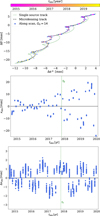 |
Fig. 1 Upper panel: tracks of the light centroid for a single source event (dotted green line) and a microlensing event with the same single source parameters (dashed black line). The blue circles correspond to Gaia along-scan measurements at different tobs, denoted by the coloured circles. Middle panel: Gaia along-scan measurements, xobs, as a function of tobs for the microlensing event. Lower panel: residuals between the simulated data with microlensing vs the model with no microlensing (Δxobs) as a function of tobs. The vertical dashed green lines correspond to t0. For all the panels, we assume the following parameters: α0 = 6.5°, δ0 = −47.3°, μα* = −2.8 mas/yr, μδ = −5.5 mas/yr, ϖ = 1 mas, u0 = −0.6, θE = 5 mas, tE = 100 days, t0 = 2017.8, πEE = −0.1, πEN = −0.1, and G0 = 14. |
Binary system parameter ranges.
2.3 GAME Filter
GAME Filter7 is a software tool developed to identify microlensing events in the Gaia dataset and obtain the parameters of the event that can help derive parameters and properties of the lensing object. The software reads xobs, xerr, Δxobs, tobs, and φobs from the Gaia data files. GAME Filter then calculates xfit, which is the deviation along φobs at tobs, for specific single source and microlensing parameters. After that, the software minimises the re-normalised microlensing unit weight error (MUWE)
![$\[\text { MUWE }=\left(\sum_{i=1}^N \frac{\left(x_{\mathrm{obs}, i}-x_{\mathrm{fit}, i}\right)^2 / x_{\mathrm{err}, i}^2}{N-11}\right)^{1 / 2},\]$](/articles/aa/full_html/2025/07/aa53525-24/aa53525-24-eq13.png) (10)
(10)
a scalar parameter that indicates the goodness of the microlensing fit, where N is the number of visits for a specific event. The goal of the minimisation is to identify parameters that bring MUWE as close as possible to its theoretical minimum value of 1. The minimisation process uses the limited memory Broyden-Fletcher-Goldfarb-Shanno (L-BFGS-B) algorithm8 to explore the parameter space and determine the optimal single source and microlensing parameters for individual events. Appendix A provides a more detailed description of the minimisation process.
Following the minimisation process, the minimiser might stop at an incorrect local minimum, failing to find the correct solution. Consequently, we established criteria for determining when an event is recovered. These criteria are based on the value of MUWE after minimisation MUWEmin, L2 optimality error Lopt (see Appendix A), initial guesses, and the boundaries imposed on individual parameters. We determined the critical values of MUWEmin and Lopt from their respective histograms as the values where histograms show a sharp decline. We considered an event to be recovered if the following criteria were met: (i) 0.9 < MUWEmin < 1.1, (ii) Lopt < 0.015, (iii) the values of πEE, πEN, and u0 differ from the initial guesses, and (iv) the values of all parameters are within the imposed boundaries.
Mock datasets.
3 Results
To assess the accuracy of GAME Filter, we generated mock datasets as described in Sect. 2.2, compared the recovered parameters to their true values, and investigated degeneracies between parameters (Sect. 3.1). We considered various scenarios, including different magnitudes (Sect. 3.2), varying numbers of Gaia visits (Sect. 3.3), detection of events with the peak microlensing signal outside of the Gaia observational window (Sect. 3.4), and false positive detections (Sect. 3.5).
In Table 3 we list all the mock datasets with their abbreviated names and properties. Furthermore, we show the percentages of recovered events Prec and the percentages of events with parameter values obtained after minimisation within 10% (20%) of their true values, denoted as P10 (P20). These metrics provide a direct measure of GAME Filter’s accuracy. Detailed discussions on these results are provided in the following subsections.
The true parameter values used to generate mock observations are: the source’s right ascension (α0), declination (δ0), proper motion in right ascension (μα*), proper motion in declination (μδ), and parallax (ϖ). The microlensing parameters are: the impact parameter (u0), the Einstein radius (θE), the time of the closest approach between the source and the lens (t0), the event timescale (tE), and the microlensing parallax components (πEE and πEN). We refer to the parameter values obtained after minimisation as α0,min, δ0,min, μα*,min, μδ,min, ϖmin, u0,min, θE,min, t0,min, tE,min, πEE,min, and πEN,min. In this paper we omit plots for α0,min and δ0,min because we imposed tight boundaries on these parameters, and they are always accurately recovered. This is motivated by the fact that the position of the observed region in the sky is always accurately known.
3.1 Parameter recovery accuracy and degeneracies
We applied GAME Filter to the lens_G14_N281_DR4 mock dataset (G0 = 14, Nv = 281, and DR4 observational run) to estimate the accuracy of parameter recovery and investigate degeneracies between parameters. We find that the percentages of recovered events are Prec = 61%, P20 = 55%, and P10 = 39% (see Table 3).
In Fig. 2 we present 2D histograms of the values of the minimised parameters as a function of their true values. A strong linear trend in all cases indicates a good correlation between the true and recovered values. The single source parameter values and t0 are well recovered for the entire parameter range. For high |u0| values, the scatter around the true values is greater due to the weaker microlensing effect, making the true values more difficult to recover. The duration of a microlensing event is typically longer than tE. Consequently, the scatter around the true values increases with tE, as longer events can extend beyond the Gaia observational time span, resulting in fewer observations and making tE more difficult to recover. Additionally, θE is more poorly constrained for larger θE, which corresponds to longer distances traversed by the lens, effectively increasing the duration of the microlensing event. Due to this, Gaia might observe a smaller fraction of the entire astrometric event.
To determine the degeneracies between the parameters, we produced the corner plots shown in Fig. 3. These plots are calculated for the ratios ℛ between the true and recovered values of the individual parameters, indicating that values close to one imply an accurate recovery of the true parameter values. Due to our method for determining initial guesses (see Appendix A), the intrinsic relationships between t0, u0, and θE are reflected in the corner plots. Specifically, the astrometric microlensing signal can exhibit one or two peaks, which influences the initial guess for t0, while the signal amplitude is affected by θE. In photometric microlensing, πEE and πEN exhibit strong degeneracies, resulting in two clusters of data in the corner plot. However, we find that astrometric data break this common degeneracy, as the relationship between πEE and πEN results in a single cluster of data points. This is because πEE and πEN determine the orientation of the ellipse, reducing the expected degeneracy.
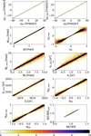 |
Fig. 2 2D histograms of values of the parameters obtained after minimisation as a function of their true values for the lens_G14_N281_DR4 mock dataset (see Tables 1 and 3). The colour bar corresponds to the number of events in individual bins. |
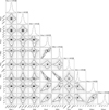 |
Fig. 3 Corner plots for ratios (ℛ) between the true and minimised values of individual parameters for recovered events in the mock dataset lens_G14_N281_DR4 (see Tables 1 and 3). |
3.2 Parameter recovery for sources with different magnitudes
We tested GAME Filter on three mock datasets, namely lens_G14_N281_DR4, lens_G16.5_N281_DR4, and lens_G19_N281_DR4, which correspond to G0 = 14, 16.5, and 19, respectively. The results of these tests are summarised in Table 3. As the magnitude increases, noise increases, and the source becomes fainter, the observed signal becomes weaker. Consequently, the number of recovered events decreases and the error of parameter estimation increases, indicated by progressively lower values of Prec, P20, and P10 as G0 increases.
In Fig. 4 we show histograms of the parameter values after minimisation for recovered events for different G0. There are several regions in the parameter space where the number of recovered events is lower: high |u0|, low θE, short tE, and long tE. For high |u0| and low θE, the microlensing signal is inherently weaker. For short and long tE, Gaia might observe only a fraction of the microlensing event: short tE due to infrequent Gaia observations and long tE because the event duration may exceed the Gaia DR4 time span. The histograms of u0 show peaks at ![$\[u_{0} \approx \sqrt{2}\]$](/articles/aa/full_html/2025/07/aa53525-24/aa53525-24-eq14.png) , consistent with Eq. (9). As the magnitude of the lensed source fades, the number of recovered events decreases, reflecting the increasing difficulty in accurately recovering parameters for fainter sources. The decrease in the number of recovered events is the most significant for regions with a weak microlensing signal. Specifically, there are no recovered events with θE ≲ 2 mas or |u0| ≳ 3 for G0 = 19.
, consistent with Eq. (9). As the magnitude of the lensed source fades, the number of recovered events decreases, reflecting the increasing difficulty in accurately recovering parameters for fainter sources. The decrease in the number of recovered events is the most significant for regions with a weak microlensing signal. Specifically, there are no recovered events with θE ≲ 2 mas or |u0| ≳ 3 for G0 = 19.
Among all simulated events, ≈80% have |u0| > 1, meaning that they do not exhibit measurable photometric but only astrometric signals. GAME Filter recovers 55% of such events for G0 = 14, while for events with photometric and astrometric signals (|u0| < 1), the recovery rate increases to 82%. For fainter source magnitudes with G0 = 16.5 and G0 = 19, the recovery rates for astrometry-only events decrease to 35.4 and 10.4%, respectively.
In Fig. 5 we show the relative errors for individual parameters after minimisation. The errors are higher for high |u0|, low θE, and short tE when the microlensing signal is weaker or more difficult to observe. The relative error of u0 is the lowest at ![$\[\left|u_{0}\right| \approx \sqrt{2}\]$](/articles/aa/full_html/2025/07/aa53525-24/aa53525-24-eq15.png) , which corresponds to the maximum microlensing deviation. When values of proper motion, geometric and microlensing parallaxes, and u0 are small, their relative errors increase drastically due to divisions by values close to 0. As G0 increases, the errors also increase, indicating that the accuracy of parameter recovery decreases for fainter sources. This change is most pronounced in regions with inherently weaker microlensing signals or fewer observations. However, GAME Filter can still recover parameters even for sources with G0 = 19 with an accuracy ≳80%, provided that θE ≳ 2 mas.
, which corresponds to the maximum microlensing deviation. When values of proper motion, geometric and microlensing parallaxes, and u0 are small, their relative errors increase drastically due to divisions by values close to 0. As G0 increases, the errors also increase, indicating that the accuracy of parameter recovery decreases for fainter sources. This change is most pronounced in regions with inherently weaker microlensing signals or fewer observations. However, GAME Filter can still recover parameters even for sources with G0 = 19 with an accuracy ≳80%, provided that θE ≳ 2 mas.
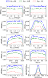 |
Fig. 4 Distributions of parameter values after minimisation for recovered events for mock datasets lens_G14_N281_DR4, lens_G16.5_N281_DR4, and lens_G19_N281_DR4, corresponding to G0 = 14 (blue), 16.5 (green), and 19 (red), respectively. The values in individual bins denote the number of recovered events within the corresponding bin range. The integral of distributions is normalised to Prec (see Table 3). |
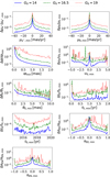 |
Fig. 5 Relative errors for recovered events for mock datasets lens_G14_N281_DR4, lens_G16.5_N281_DR4, and lens_G19_N281_DR4, corresponding to G0 = 14 (blue), 16.5 (green), and 19 (red). The errors are calculated as the difference between the minimised and true parameter values divided by the minimised parameter values. The error values are first binned and then calculated as the mean in each bin. |
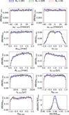 |
Fig. 6 Distributions of parameter values after minimisation for recovered events for mock datasets lens_G14_N281_DR4, lens_G14_N209_DR4, and lens_G14_N91_DR4 corresponding to Nv = 281 (blue), 209 (green), and 91 (red). The values in individual bins denote the number of recovered events within the corresponding bin range. The integral of distributions is normalised to Prec (see Table 3). |
3.3 Parameter recovery for events with different numbers of Gaia visits
We tested GAME Filter on mock datasets lens_G14_N281_DR4, lens_G14_N209_DR4, and lens_G14_N91_DR4, which correspond to regions with different numbers of Gaia visits Nv = 281, 209, and 91. The results are summarised in Table 3, showing that the changes in Nv do not significantly affect Prec. Additionally, P20 and P10 remain unaffected when Nv decreases to at least 209. When Nv is further reduced to 91, P20 and P10 show only a ≈5% change.
In Fig. 6 we show histograms of the parameter values after minimisation for recovered events for different Nv. These histograms indicate that Nv does not significantly affect the recovery of parameter values, as long as Nv ≳ 90. The most noticeable difference is in the values of MUWEmin, which spread more broadly as Nv decreases.
We also calculated the relative errors for individual parameters after minimisation and found that the errors increase slightly with decreasing Nv. Since the impact is not significant, this indicates that GAME Filter performs robustly even with fewer observations. However, a higher number of observations generally improves the accuracy of parameter recovery.
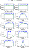 |
Fig. 7 Distributions of parameter values after minimisation for recovered events for mock datasets lens_G14_N281_DR4 and lens_G14_N209_extended, corresponding to t0 ∈ [2014.5, 2020] yr and t0 ∈ [2010, 2024] yr, respectively. The values in individual bins denote the number of recovered events within the corresponding bin range. The integral of distributions is normalised to Prec (see Table 3). |
3.4 Parameter recovery for events with the maximum microlensing signal beyond Gaia’s observational run
We tested GAME Filter on mock datasets lens_G14_N281_DR4 and lens_G14_N281_extend, which correspond to mock dataset within Gaia DR4 with t0 ∈ [2014.5, 2020] yr and mock dataset extending beyond DR4 with t0 ∈ [2010, 2024] yr, respectively. The results of these tests are summarised in Table 3. We see that increasing the t0 range decreases Prec, P20, and P10 by ≈15, ≈20, and 15%, respectively.
In Fig. 7 we show histograms of the parameter values after minimisation for recovered events for different ranges of t0. As t0 extends beyond the DR4 run, Prec decreases. This is because a significant part of the microlensing event can fall outside the Gaia observation time span, reducing the amount of available data and making parameter recovery more challenging. This effect is most apparent for events with a short tE. Furthermore, the histogram of u0 transitions from a bimodal distribution to a single peak as the t0 range increases. There are also fewer recovered events for large θE, as larger θE corresponds to longer lens paths and event durations, which means that a smaller portion of the event is observed if t0 is outside the DR4 time span. We also see fewer recovered events for microlensing parallaxes close to −1 and 1, since these events have more variations, or ‘wiggles’ in the observed astrometric signal, which makes the parameter recovery more challenging. We discuss the physical mechanism for these differences in Sect. 4.1.
In Fig. 8 we show the relative errors for individual parameters after minimisation. The errors are generally higher for all parameters when the t0 range extends beyond the DR4 run, indicating that the timing of the microlensing event relative to the Gaia observational run affects parameter recovery accuracy. This effect is more pronounced for events with short tE, which are less likely to be fully observed if t0 is outside the DR4 time span.
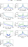 |
Fig. 8 Relative errors for recovered events for mock datasets lens_G14_N281_DR4 and lens_G14_N209_extended, corresponding to t0 ∈ [2014.5, 2020] yr and t0 ∈ [2010, 2024] yr, respectively. The errors are calculated as the difference between the minimised and true parameter values divided by the minimised parameter values. The error values are first binned and then calculated as the mean in each bin. |
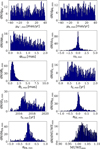 |
Fig. 9 Distributions of parameter values after minimisation for binary system events in the binary_G14_N281_DR4 mock dataset (see Tables 2 and 3). The values in individual bins denote the number of recovered events within the corresponding bin range. The integral of distributions is normalised to Prec (see Table 3). |
3.5 Parameter recovery for the false positive detections
To evaluate the performance of GAME Filter in distinguishing microlensing events from other astrometric phenomena, we tested it on the binary_G14_N281_DR4 mock dataset, which corresponds to binary system events. The results of these tests are summarised in Table 3. We determined that the percentage of false positive identifications is very low, with Prec = 5% and P20 = P10 = 0%.
In Fig. 9 we show histograms of the parameter values after minimisation for recovered binary events. Histograms indicate that false positive events typically have low values of θE and high values of |u0|, suggesting that they are interpreted as weak microlensing events. These results demonstrate that while GAME Filter is highly effective in identifying microlensing events, a small percentage of binary events with a weak astrometric signal may still be misinterpreted as microlensing events.
4 Discussion
4.1 Parameter recovery accuracy
Given the high number of recovered events and low parameter estimation errors, we find that GAME Filter tends to perform with a high level of accuracy. However, there are several challenges related to precisely recovering parameters: (i) the effect of microlensing parameters on the microlensing ellipse, (ii) the time of closest approach between the lens and the source t0, (iii) source magnitude G0, (iv) the number of Gaia visits Nv, and (v) the probability of false positive detections.
(i) The parameters u0 and θE define the shape and size of this ellipse. A larger θE results in a proportionally larger ellipse, which increases both the magnitude of the astrometric shift and the duration of the event. When u0 is close to zero, the ellipse becomes more elongated, resembling a straight line, while an increase in u0 makes the ellipse more circular. The strongest microlensing signal occurs at ![$\[u_{0}=\sqrt{2} \theta_{\mathrm{E}}\]$](/articles/aa/full_html/2025/07/aa53525-24/aa53525-24-eq16.png) and t0, where the ellipse reaches its maximum size. This is reflected in the percentage of events recovered for specific regions in the parameter space (see Figs. 4, 6, and 7). For high |u0| and low θE, the microlensing signal is weaker, leading to a decrease in the number of recovered events. Furthermore, high values of θE can cause a decrease in the number of recovered events due to the longer lens path and duration of the event. This may result in a significant part of the event falling outside the Gaia DR4 observational time span, making parameter estimation more challenging. This effect is analogous for long tE.
and t0, where the ellipse reaches its maximum size. This is reflected in the percentage of events recovered for specific regions in the parameter space (see Figs. 4, 6, and 7). For high |u0| and low θE, the microlensing signal is weaker, leading to a decrease in the number of recovered events. Furthermore, high values of θE can cause a decrease in the number of recovered events due to the longer lens path and duration of the event. This may result in a significant part of the event falling outside the Gaia DR4 observational time span, making parameter estimation more challenging. This effect is analogous for long tE.
Gaia observations along the microlensing ellipse are not evenly spaced in distance. For small u0, the observations are more evenly distributed on the sky, whereas for large u0, there are fewer observations near the maximum of the microlensing deviation. Due to this, Gaia predominantly observes the astrometric deviation along the edges of the ellipse rather than at its maximum when t0 is outside of DR4, increasing the difficulty of estimating the parameters for high u0. This effect is seen in Fig. 7, where the histogram of u0 changes from a bimodal to a single peak distribution as the range of t0 extends beyond the Gaia observational window.
The microlensing ellipse is also affected by πEE and πEN, which determine both the orientation of the ellipse in the sky and the parallax of the lens πL (see Eq. (7)). Higher values of πEE and πEN lead to a larger πE and consequently to a higher πL, assuming a fixed ϖ. When the lens is closer to the observer, its parallactic motion introduces more variations in the observed astrometric signal. This added complexity makes parameter estimation more challenging, requiring more measurements to accurately constrain the parameters. This effect is particularly pronounced when t0 lies outside of the Gaia observational window, as shown in Fig. 7.
(ii) Microlensing events can span several years, and many such events have t0 beyond the Gaia DR4 observation time span. Consequently, Gaia may often miss the maximum of the astrometric microlensing signal. However, we find that when t0 lies outside of Gaia DR4, parameters can still be recovered. The percentage of recovered events decreases by ≈15% (see Table 3) and the parameter estimation errors for such events are higher (see Fig. 8). This is most evident for events with short tE, which are less likely to be observed, as seen in Fig. 7.
(iii) When simulating Gaia mock observations, noise is introduced by scattering the observations along the scanning angle based on the magnitude-dependent error bars, thus reflecting true Gaia measurements. Due to this, the scatter in Gaia’s along-scan measurements increases with fainter G0 as shown in Fig. 10. This increased scatter makes it more challenging to accurately recover parameters, as seen in Figs. 4, 6, and 7. This effect is most pronounced in regions with high |u0| and low θE, where the microlensing signal is already weak. Specifically, for θE ≳ 2.5 mas, the parameter is recovered with a relative error of ≲20% even when G0 = 19. However, for θE ≲ 2.5 mas, the error estimation can reach an order of unity if G0 = 19.
(iv) In Gaia DR4, different regions in the sky are observed on average ≈100 times. We find that for Nv ≥ 91, a decrease in Nv leads to only a slight increase in relative errors. For example, when Nv decreases from 281 to 91, the percentage of parameters with their estimated values within 10% of their true values decreases by ≈5% (see Table 3).
(v) Gaia observes various types of astrometric phenomena, including single-star motions, binary systems, microlensing, and other transient events9. In general, binaries produce periodic astrometric signals that are easily distinguishable from transient microlensing events. However, a subset of binaries characterised by long orbital periods and large semi-major axes can produce transient signals mimicking microlensing. We adopted uniform orbital period distributions from 0.01 to 5 years (see Table 2) and found that ~5% of binary events are misclassified as microlensing events for G0 = 1410. However, realistic binary populations differ from uniform distributions. Observations of DR3 binaries show that orbital periods typically peak around 500 days (Halbwachs et al. 2023), while predictions for Gaia DR4 suggest a peak around 2.5–3 years (El-Badry et al. 2024). Thus, our choice likely under-represents short-period binaries and over-represents longer-period binaries. Despite this bias, we find that the false positives exhibit uniformly distributed orbital parameters, suggesting that statistical noise rather than particular orbital configurations is the dominant cause of confusion.
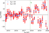 |
Fig. 10 Gaia along-scan measurements (xobs) as a function of tobs for G0 = 14 (blue circles) and 19 (red diamonds). The vertical dashed green lines correspond to t0. We assume the same single source and microlensing parameters as in Fig. 1. |
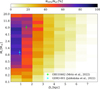 |
Fig. 11 2D histogram showing the sensitivity of GAME Filter as functions of DL and ML. The sensitivity, indicated by the colour bar, is calculated as the ratio N20%/Nall · ML is sampled logarithmically between 0.1 and 20 M⊙, and DL is sampled uniformly between 0.1 and 7.9 kpc. The cyan and green circles with error bars indicate two microlensing events, OB110462 (ML = 7.1 ± 1.3 M⊙, DL = 1.5 ± 0.1 kpc; Mróz et al. 2022) and GDR3-001 (ML = 1.0 ± 0.2 M⊙, DL = 0.9 ± 0.1 kpc; Jabłońska et al. 2022), respectively. |
4.2 Constraining the lens properties
To evaluate the sensitivity of the GAME Filter to detect lenses in the Milky Way with varying distances DL and masses ML, we applied the GAME Filter to a new mock dataset of Nall = 50 000 microlensing events. For each event, ML is randomly selected from a logarithmically spaced interval between 0.1 and 20 M⊙, and DL is uniformly sampled from 0.1 to 7.9 kpc. The angle between the microlensing parallax components πEE and πEN is selected from a uniform distribution between 0 and 2π. Additional parameters are sampled uniformly within their respective ranges (see Table 1) with the exception of u0 where we changed the range to −3 to 3. Using these values, the microlensing parallax πE and the angular Einstein radius θE are calculated from πS, ML, and DL (see Eqs. (1) and (7)). GAME Filter recovers N20% = 11 456 events with parameter values minimised within 20% of their true values, corresponding to approximately 22% of Nall.
In Fig. 11 we present a 2D histogram showing GAME Filter’s sensitivity expressed as the ratio N20%/Nall across DL and ML parameter space. As expected, our algorithm demonstrates the highest sensitivity for nearby lenses with high masses, where the astrometric microlensing signal is strongest. For lenses with DL ≲ 1 kpc and ML ≳ 1 M⊙, the sensitivity is 70–80%. For ML ~ 20 M⊙, the sensitivity drops to ≈50%. This is caused by a large Einstein Radius θE and hence a very long event timescale. Consequently, longer observation times are required to capture the full event, limiting GAME Filter’s ability to constrain the lens properties accurately within Gaia DR4 time frame. At distances of 4–6 kpc, the sensitivity ranges from 10–20% for lenses with ML ≳ 2 M⊙. For DL > 4 kpc and ML < 2 M⊙, the sensitivity drops below 10%, reflecting the significantly weaker astrometric microlensing signal.
Figure 11 shows the first two microlensing events studied using combined photometry and astrometry: OB110462 (Mróz et al. 2022) and GDR3-001 (Jabłońska et al. 2022). Both events lie within regions of high sensitivity, demonstrating the GAME Filter’s ability to detect similar events.
4.3 Caveats
When generating astrometric events, we assumed a uniform distribution of their parameters, which does not accurately reflect their true distributions in the Milky Way (e.g. Mao & Paczyński 1996). However, the primary aim of our study is not to model the Galaxy accurately but to validate the performance and accuracy of GAME Filter across a wide range of parameters. Using uniform distributions allowed us to test the filter under diverse conditions and identify specific regions in the parameter space where GAME Filter may underperform. In such cases, deviations from a uniform recovery distribution can highlight areas where parameter estimation is less accurate or more difficult.
The optimisation process in GAME Filter may occasionally converge to a local minimum instead of the global minimum, potentially leading to incorrect parameter estimates. To mitigate this, we used multiple initial guesses for parameters u0, πEE, and πEN for which we lack initial estimates (see Appendix A). Specifically, we used ten different values for u0 and five different values for both πEE and πEN within a defined interval. Although this approach improves parameter recovery accuracy, it does not cover the entire parameter space. To evaluate this, we further tested GAME Filter on a subset of lens_G14_N281_DR4 mock dataset with 5000 events, increasing the number of initial guesses for u0, πEE, and πEN to 13,7, and 7, respectively. We also applied this approach to the parameters θE, t0, and tE, where we considered five different values for individual parameters. We find no significant improvement compared to our original method. Due to this, we conclude that our original approach strikes a balance between computational efficiency, thorough parameter space exploration, and accurate parameter estimation.
Another limitation of GAME Filter is the assumption of negligible blending in the observed data. Blending occurs when light from the source combines with light from the lens (and/or a nearby unresolvable source), distorting the apparent motion of the light centroid and potentially leading to inaccurate microlensing parameter estimates. To accurately account for this effect, the blending parameter fbl ∈ [0, 1] is required. The measured Gaia parallax πG in a simple case of source and luminous lens before or after the event (when the amplification is 1) can be expressed as
![$\[\pi_{\mathrm{G}}=\varpi f_{\mathrm{bl}}+\pi_{\mathrm{L}}\left(1-f_{\mathrm{bl}}\right),\]$](/articles/aa/full_html/2025/07/aa53525-24/aa53525-24-eq17.png) (11)
(11)
and similarly for the proper motions. When fbl is near 1, the observed signal mainly reflects the motion of the source, while values close to zero reflect the motion of the lens. Intermediate values represent mixed cases where accurate estimation of the lens parallax requires additional source distance measurements, for example spectroscopic typing. In our study, we considered fbl = 1 to determine the lower boundary for the Einstein radius, θE. This, in turn, establishes a minimum estimate for both the distance and mass of the lens. If fbl were less than 1, indicating a significant contribution of light from the lens, the actual distance and mass would likely be higher than the values estimated under this assumption.
5 Conclusions
The Gaia mission provides an unprecedented opportunity to observe microlensing events solely as astrometric anomalies. Although photometric detection has its merits, this study focused on the identification of events only through the astrometric data. To leverage the astrometric precision of Gaia, we developed GAME Filter, a software capable of identifying microlensing events and deriving the properties of the lensing objects that cause them. The main conclusions of our study are the following.
GAME Filter can be used to characterise lenses with astrometry-only data for lens masses ranging from approximately 0.1–20 M⊙ and distances of up to ≈7 kpc. While the sensitivity decreases with increasing distance and decreasing lens mass, the microlensing events currently being studied in the literature fall within regions of high sensitivity.
Values of MUWE and the L2 optimality error after minimisation can be used to filter recovered events for which GAME Filter reached the desired convergence.
The recovery of true microlensing parameters is more challenging in specific regions of the parameter space, such as low-θE and high-|u0| areas, due to the weaker microlensing effect resulting in higher scatter around true values and higher parameter estimation errors.
Microlensing parameters are more difficult to recover for very short- and very long-duration events since Gaia might observe only a fraction of a microlensing event.
There are no strong degeneracies for recovered events. Additionally, astrometry breaks the common degeneracy between the north and east components of the microlensing parallax present in photometry-only microlensing.
As the magnitude increases, the observed signal becomes fainter, decreasing the number of recovered events and increasing the parameter estimation error. We find that even for G0 = 19, parameters can be recovered for θE ≳ 2 mas.
Observing regions with different numbers of Gaia visits does not significantly affect the number and parameter estimation errors of recovered events, provided the number of visits is above average, i.e. ≳90.
Even if the peak of the microlensing event is outside of the Gaia observational run, microlensing parameters can still be recovered, although with higher errors.
Binary systems represent a potential contaminant for GAME Filter’s performance. We find that only ≈5% of binary events get falsely identified as weak microlensing events for G0 = 14. However, we assumed uniform orbital parameter distributions, likely overestimating the confusion rate by underrepresenting short-period binaries and over-representing long-period binaries. Nevertheless, we find that the false positives exhibit a uniform distributions of parameters, suggesting that statistical noise rather than particular orbital configurations is the dominant cause of confusion.
We have presented our results for Gaia DR4. GAME Filter demonstrates robust performance in detecting astrometric microlensing events. For DR5, we expect a similar overall performance. Additionally, we expect that the longer observing time will allow the detection of longer-duration events, particularly those with larger θE, which may have been missed in DR4 due to insufficient sampling. Such events are expected to be less frequent, as lenses with high masses are inherently rarer. However, these events would be of special astrophysical interest as they are more likely to involve massive black holes. Additionally, we note that a quantitative estimate of the number of astrometric microlensing events detectable in DR4 requires detailed simulations with realistic Galactic population models. Such an estimate is beyond the scope of this paper. We plan to provide detailed predictions of event rates using realistic populations in a future study (Kaczmarek, et al., in prep.).
The work presented here suggests that astrometric data can not only complement photometric detections but also enable microlensing detections and the determination of lens parameters independently, even in the absence of photometric signals. Therefore, this study paves the way for future astrometric investigations that fully leverage the capabilities of Gaia data.
Data availability
The software to generate mock Gaia observations and GAME Filter are available at https://github.com/tajjankovic/GAME-Filter/.
Acknowledgements
T.J., A.G., Ł.W., T.P., M.K., and M.L. acknowledge the financial support from the European Space Agency PRODEX Experiment Arrangement GAME. T. J., A. G., T.P., M.B., and M.K. acknowledge the financial support from the Slovenian Research Agency (research core funding P1-0031, infrastructure program I0-0033, and project grants Nos. J1-8136, J1-2460, N1-0344). Ł.W. acknowledges the funding from the European Union’s research and innovation programme under grant agreements Nos. 101004719 (ORP) and 101131928 (ACME). We acknowledge ESA Gaia and the many researchers from Gaia DPAC for their valuable contributions and expertise at different phases of this project. Researcher T.J. conducts his research under the Marie Skłodowska-Curie Actions – COFUND project, which is co-funded by the European Union (Physics for Future – Grant Agreement No. 101081515). Z.K. is a Fellow of the International Max Planck Research School for Astronomy and Cosmic Physics at the University of Heidelberg (IMPRS-HD). The following software was used in this work: astromet (https://github.com/zpenoyre/astromet.py), jaxtromet (https://github.com/maja-jablonska/jaxtromet.py), jaxopt (Blondel et al. 2021), Matplotlib (Hunter 2007).
Appendix A GAME Filter
GAME Filter11 is a software tool developed to identify microlensing events in the Gaia dataset and derive the properties of the lensing objects. GAME Filter processes N events (the number of Gaia data files, typically in .parquet format) in parallel. Each CPU or GPU core reads a file containing the data for an event. Specifically, the software reads xobs, xerr, Δxobs, tobs, and φobs. GAME Filter calculates xfit, the deviation along φobs at tobs, for specific single source and microlensing parameters. The software then minimises a scalar parameter MUWE (see Eq. (10)), which indicates the goodness of the microlensing fit. The minimisation process utilises the L-BFGS-B algorithm to explore the parameter space and determine the optimal single source and microlensing parameters for individual events. It saves the best-fit results to disk and repeats these steps for every file.
In the following, we describe a method for obtaining initial guesses for individual parameters ![$\[\alpha_{0}^{0}, \delta_{0}^{0}, \mu_{\alpha^{\star}}^{0}, \mu_{\delta}^{0}, \varpi^{0}, u_{0}^{0}, \theta_{\mathrm{E}}^{0}, t_{0}^{0}, t_{\mathrm{E}}^{0}, \pi_{\mathrm{EE}}^{0}\]$](/articles/aa/full_html/2025/07/aa53525-24/aa53525-24-eq18.png) and
and ![$\[\pi_{\mathrm{EN}}^{0}\]$](/articles/aa/full_html/2025/07/aa53525-24/aa53525-24-eq19.png) , and the main steps of the minimisation process.
, and the main steps of the minimisation process.
A.1 Initial guess
The single source initial guess values for ![$\[\alpha_{0}^{0}, \delta_{0}^{0}, \mu_{\alpha^{\star}}^{0}, \mu_{\delta}^{0}\]$](/articles/aa/full_html/2025/07/aa53525-24/aa53525-24-eq20.png) , and ϖ0 were obtained from the Gaia files, corresponding to the values obtained from a single source fit. In addition, we used
, and ϖ0 were obtained from the Gaia files, corresponding to the values obtained from a single source fit. In addition, we used ![$\[u_{0}^{0}=0.01, \pi_{\mathrm{EE}}^{0}=0.01\]$](/articles/aa/full_html/2025/07/aa53525-24/aa53525-24-eq21.png) , and
, and ![$\[\pi_{\mathrm{EN}}^{0}=0.01\]$](/articles/aa/full_html/2025/07/aa53525-24/aa53525-24-eq22.png) . We obtained the initial guesses
. We obtained the initial guesses ![$\[\theta_{\mathrm{E}}^{0}, t_{0}^{0}\]$](/articles/aa/full_html/2025/07/aa53525-24/aa53525-24-eq23.png) and
and ![$\[t_{\mathrm{E}}^{0}\]$](/articles/aa/full_html/2025/07/aa53525-24/aa53525-24-eq24.png) by fitting a Gaussian function to the histograms of residuals Δxobs, included in the Gaia data files, using the curve_fit function from the scipy.optimize module in the S*ciPy library. This is shown in Fig. A.1 (top panel). We relate
by fitting a Gaussian function to the histograms of residuals Δxobs, included in the Gaia data files, using the curve_fit function from the scipy.optimize module in the S*ciPy library. This is shown in Fig. A.1 (top panel). We relate ![$\[\theta_{\mathrm{E}}^{0}\]$](/articles/aa/full_html/2025/07/aa53525-24/aa53525-24-eq25.png) to the maximum Gaussian
to the maximum Gaussian ![$\[\Delta x_{\text {obs, } \max }, t_{0}^{0}\]$](/articles/aa/full_html/2025/07/aa53525-24/aa53525-24-eq26.png) to the time tobs of the maximum of the Gaussian, and
to the time tobs of the maximum of the Gaussian, and ![$\[t_{\mathrm{E}}^{0}\]$](/articles/aa/full_html/2025/07/aa53525-24/aa53525-24-eq27.png) to the standard deviation of the Gaussian. We find that the relation between θE and Δxobs,max can be approximated as
to the standard deviation of the Gaussian. We find that the relation between θE and Δxobs,max can be approximated as ![$\[\theta_{\mathrm{E}}^{0} \approx 3 \Delta x_{\mathrm{obs}, \max }-2.25\]$](/articles/aa/full_html/2025/07/aa53525-24/aa53525-24-eq28.png) . We show this correlation in Fig. A.1 (lower panel) for different u0. We see that the change in u0 does not significantly affect the relation between θE and Δxobs,max.
. We show this correlation in Fig. A.1 (lower panel) for different u0. We see that the change in u0 does not significantly affect the relation between θE and Δxobs,max.
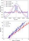 |
Fig. A.1 Upper panel: Residuals calculated as the absolute value of the mean of individual bins (solid lines) for θE = 1 mas (red) and θE = 3 mas (blue). We used 30 equally spaced bins in tobs. Histograms are normalised to 1. We assume |
![$\[\alpha=6.49^{\circ}, \delta=-47.6^{\circ}, \varpi=1, \mu_{\alpha}^{*}=0, \mu_{\delta}=0, u_{0}=0.5, t_{0}=2017.3\]$](/articles/aa/full_html/2025/07/aa53525-24/aa53525-24-eq29.png)
![$\[\theta_{\mathrm{E}}^{0}\]$](/articles/aa/full_html/2025/07/aa53525-24/aa53525-24-eq30.png)
A.2 Minimisation steps
We implemented several steps to improve the accuracy of GAME Filter. These criteria are based on the L2 optimality error Lopt, initial guesses, and the boundaries imposed on individual parameters. Lopt, often used in optimisation problems, determines the accuracy of the minimiser by defining the change during subsequent iterations in the parameter space, where values closer to zero indicate a more accurate solution. We find that using minimisation methods with the bounds and changing the initial guesses ![$\[u_{0}^{0}, \pi_{\mathrm{EE}}^{0}\]$](/articles/aa/full_html/2025/07/aa53525-24/aa53525-24-eq31.png) and
and ![$\[\pi_{\mathrm{EN}}^{0}\]$](/articles/aa/full_html/2025/07/aa53525-24/aa53525-24-eq32.png) significantly improves the accuracy of GAME Filter. Based on this, the main minimisation steps are as follows.
significantly improves the accuracy of GAME Filter. Based on this, the main minimisation steps are as follows.
Calculate Lopt after minimisation.
-
If Lopt is higher than a threshold value Lthresh = 0.01, change
![$\[u_{0}^{0}, \pi_{\mathrm{EE}}^{0}\]$](/articles/aa/full_html/2025/07/aa53525-24/aa53525-24-eq33.png) and
and ![$\[\pi_{\mathrm{EN}}^{0}\]$](/articles/aa/full_html/2025/07/aa53525-24/aa53525-24-eq34.png) . We determined Lthresh = 0.01 from Lopt histograms as the value where 90% of the data falls below this threshold, effectively removing the top 10% of values in the distribution tails. This is also shown in Fig. A.2 (lower panel).
. We determined Lthresh = 0.01 from Lopt histograms as the value where 90% of the data falls below this threshold, effectively removing the top 10% of values in the distribution tails. This is also shown in Fig. A.2 (lower panel).- (a)
For
![$\[u_{0}^{0}\]$](/articles/aa/full_html/2025/07/aa53525-24/aa53525-24-eq35.png) , use ten different values from an evenly spaced interval of
, use ten different values from an evenly spaced interval of ![$\[u_{0}^{0}\]$](/articles/aa/full_html/2025/07/aa53525-24/aa53525-24-eq36.png) ∈ [−5, 5].
∈ [−5, 5]. - (b)
For
![$\[\pi_{\mathrm{EE}}^{0}\]$](/articles/aa/full_html/2025/07/aa53525-24/aa53525-24-eq37.png) and
and ![$\[\pi_{\mathrm{EN}}^{0}\]$](/articles/aa/full_html/2025/07/aa53525-24/aa53525-24-eq38.png) , use five different values from an evenly spaced interval of
, use five different values from an evenly spaced interval of ![$\[\pi_{\mathrm{EE}}^{0}, \pi_{\mathrm{EN}}^{0} \in[-1,1]\]$](/articles/aa/full_html/2025/07/aa53525-24/aa53525-24-eq39.png) .
.
- (a)
Stop the iteration if Lopt < Lthresh. Otherwise, keep the parameters with the lowest Lopt.
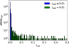 |
Fig. A.2 Distribution of Lopt for the lens_G14_N281_DR4 mock dataset (see Tables 1 and 3). Blue and green denote events with Lopt ≤ 0.01 and Lopt > 0.01, respectively. The values in individual bins denote the number of events within the corresponding bin range. |
References
- Belokurov, V. A., & Evans, N. W. 2002, MNRAS, 331, 649 [NASA ADS] [CrossRef] [Google Scholar]
- Blondel, M., Berthet, Q., Cuturi, M., et al. 2021, arXiv e-prints [arXiv:2105.15183] [Google Scholar]
- Bond, I., Abe, F., Dodd, R., et al. 2001, MNRAS, 327, 868 [NASA ADS] [CrossRef] [Google Scholar]
- Chen, I.-K., Kongsore, M., & Tilburg, K. V. 2023, J. Cosmol. Astropart. Phys., 2023, 037 [Google Scholar]
- Dominik, M., & Sahu, K. C. 2000, ApJ, 534, 213 [CrossRef] [Google Scholar]
- Dong, S., Mérand, A., Delplancke-Ströbele, F., Gould, A., & Zang, W. 2019, The Messenger, 178, 45 [NASA ADS] [Google Scholar]
- Einstein, A. 1936, Science, 84, 506 [NASA ADS] [CrossRef] [Google Scholar]
- El-Badry, K., Lam, C., Holl, B., et al. 2024, Open J. Astrophys., 7, 100 [Google Scholar]
- Fardeen, J., McGill, P., Perkins, S. E., et al. 2024, ApJ, 965, 138 [Google Scholar]
- Gaia Collaboration (Prusti, T., et al.) 2016, A&A, 595, A1 [NASA ADS] [CrossRef] [EDP Sciences] [Google Scholar]
- Gaia Collaboration (Brown, A. G. A., et al.) 2018, A&A, 616, A1 [NASA ADS] [CrossRef] [EDP Sciences] [Google Scholar]
- Gaia Collaboration (Smart, R. L., et al.) 2021, A&A, 649, A6 [EDP Sciences] [Google Scholar]
- Gaia Collaboration (Arenou, F., et al.) 2023, A&A, 674, A34 [CrossRef] [EDP Sciences] [Google Scholar]
- Gould, A. 2004, ApJ, 606, 319 [NASA ADS] [CrossRef] [Google Scholar]
- Halbwachs, J.-L., Pourbaix, D., Arenou, F., et al. 2023, A&A, 674, A9 [NASA ADS] [CrossRef] [EDP Sciences] [Google Scholar]
- Hog, E., Novikov, I. D., & Polnarev, A. G. 1995, A&A, 294, 287 [NASA ADS] [Google Scholar]
- Hunter, J. D. 2007, Comput. Sci. Eng., 9, 90 [NASA ADS] [CrossRef] [Google Scholar]
- Jabłońska, M., Wyrzykowski, Ł., Rybicki, K. A., et al. 2022, A&A, 666, L16 [NASA ADS] [CrossRef] [EDP Sciences] [Google Scholar]
- Klüter, J., Bastian, U., Demleitner, M., & Wambsganss, J. 2018, A&A, 620, A175 [NASA ADS] [CrossRef] [EDP Sciences] [Google Scholar]
- Klüter, J., Bastian, U., Demleitner, M., & Wambsganss, J. 2022, AJ, 163, 176 [CrossRef] [Google Scholar]
- Mao, S., & Paczyński, B. 1996, ApJ, 473, 57 [NASA ADS] [CrossRef] [Google Scholar]
- McGill, P., Smith, L. C., Evans, N. W., Belokurov, V., & Smart, R. L. 2018, MNRAS, 478, L29 [NASA ADS] [CrossRef] [Google Scholar]
- Miralda-Escude, J. 1996, ApJ, 470, L113 [Google Scholar]
- Miyamoto, M., & Yoshii, Y. 1995, AJ, 110, 1427 [NASA ADS] [CrossRef] [Google Scholar]
- Mróz, P., Udalski, A., & Gould, A. 2022, ApJ, 937, L24 [CrossRef] [Google Scholar]
- Paczynski, B. 1986, ApJ, 301, 503 [NASA ADS] [CrossRef] [Google Scholar]
- Penoyre, Z., Belokurov, V., & Evans, N. W. 2022, MNRAS, 513, 2437 [NASA ADS] [CrossRef] [Google Scholar]
- Refsdal, S. 1964, MNRAS, 128, 307 [NASA ADS] [CrossRef] [Google Scholar]
- Sahu, K. C., Anderson, J., Casertano, S., et al. 2017, Science, 356, 1046 [Google Scholar]
- Sahu, K. C., Anderson, J., Casertano, S., et al. 2022, ApJ, 933, 83 [Google Scholar]
- Su, J., Wang, J., Zhang, Y., Cheng, X., & Yang, L. 2023, MNRAS, 527, 1177 [Google Scholar]
- Udalski, A. 2003, Acta Astron., 53, 291 [NASA ADS] [Google Scholar]
- Walker, M. A. 1995, ApJ, 453, 37 [NASA ADS] [CrossRef] [Google Scholar]
- Wyrzykowski, Ł., Kruszyńska, K., Rybicki, K. A., et al. 2023, A&A, 674, A23 [NASA ADS] [CrossRef] [EDP Sciences] [Google Scholar]
- Zurlo, A., Gratton, R., Mesa, D., et al. 2018, MNRAS, 480, 236 [NASA ADS] [CrossRef] [Google Scholar]
These Nv values correspond to regions most frequently visited by Gaia (281 visits), regions with an approximately average visit number (91 visits), and intermediate regions (209 visits). We determined Nv using the scanninglaw Python package (https://github.com/gaiaverse/scanninglaw), as this information is not available in GOST. However, since this package does not provide data for Gaia DR4, we used Nv for Gaia DR3.
Unresolved fixed-separation binaries where one star is photometrically variable could represent another source of false positives. However, these can typically be identified through photometric observations. Given Gaia DR4’s observational baseline of approximately 5.5 years, most variable sources will exhibit multiple astrometric or photometric peaks within this timeframe, distinguishing them from microlensing events. Nonetheless, transient phenomena such as novae could still potentially mimic microlensing signatures.
For fainter sources, astrometric uncertainties increase, potentially elevating the rate of false positives. However, since the GAME Filter preferentially detects high signal-to-noise events at fainter magnitudes, these two effects largely balance out, resulting in a misclassification rate that does not significantly depend on magnitude.
All Tables
All Figures
|
Fig. 1 Upper panel: tracks of the light centroid for a single source event (dotted green line) and a microlensing event with the same single source parameters (dashed black line). The blue circles correspond to Gaia along-scan measurements at different tobs, denoted by the coloured circles. Middle panel: Gaia along-scan measurements, xobs, as a function of tobs for the microlensing event. Lower panel: residuals between the simulated data with microlensing vs the model with no microlensing (Δxobs) as a function of tobs. The vertical dashed green lines correspond to t0. For all the panels, we assume the following parameters: α0 = 6.5°, δ0 = −47.3°, μα* = −2.8 mas/yr, μδ = −5.5 mas/yr, ϖ = 1 mas, u0 = −0.6, θE = 5 mas, tE = 100 days, t0 = 2017.8, πEE = −0.1, πEN = −0.1, and G0 = 14. |
| In the text | |
|
Fig. 2 2D histograms of values of the parameters obtained after minimisation as a function of their true values for the lens_G14_N281_DR4 mock dataset (see Tables 1 and 3). The colour bar corresponds to the number of events in individual bins. |
| In the text | |
|
Fig. 3 Corner plots for ratios (ℛ) between the true and minimised values of individual parameters for recovered events in the mock dataset lens_G14_N281_DR4 (see Tables 1 and 3). |
| In the text | |
|
Fig. 4 Distributions of parameter values after minimisation for recovered events for mock datasets lens_G14_N281_DR4, lens_G16.5_N281_DR4, and lens_G19_N281_DR4, corresponding to G0 = 14 (blue), 16.5 (green), and 19 (red), respectively. The values in individual bins denote the number of recovered events within the corresponding bin range. The integral of distributions is normalised to Prec (see Table 3). |
| In the text | |
|
Fig. 5 Relative errors for recovered events for mock datasets lens_G14_N281_DR4, lens_G16.5_N281_DR4, and lens_G19_N281_DR4, corresponding to G0 = 14 (blue), 16.5 (green), and 19 (red). The errors are calculated as the difference between the minimised and true parameter values divided by the minimised parameter values. The error values are first binned and then calculated as the mean in each bin. |
| In the text | |
|
Fig. 6 Distributions of parameter values after minimisation for recovered events for mock datasets lens_G14_N281_DR4, lens_G14_N209_DR4, and lens_G14_N91_DR4 corresponding to Nv = 281 (blue), 209 (green), and 91 (red). The values in individual bins denote the number of recovered events within the corresponding bin range. The integral of distributions is normalised to Prec (see Table 3). |
| In the text | |
|
Fig. 7 Distributions of parameter values after minimisation for recovered events for mock datasets lens_G14_N281_DR4 and lens_G14_N209_extended, corresponding to t0 ∈ [2014.5, 2020] yr and t0 ∈ [2010, 2024] yr, respectively. The values in individual bins denote the number of recovered events within the corresponding bin range. The integral of distributions is normalised to Prec (see Table 3). |
| In the text | |
|
Fig. 8 Relative errors for recovered events for mock datasets lens_G14_N281_DR4 and lens_G14_N209_extended, corresponding to t0 ∈ [2014.5, 2020] yr and t0 ∈ [2010, 2024] yr, respectively. The errors are calculated as the difference between the minimised and true parameter values divided by the minimised parameter values. The error values are first binned and then calculated as the mean in each bin. |
| In the text | |
|
Fig. 9 Distributions of parameter values after minimisation for binary system events in the binary_G14_N281_DR4 mock dataset (see Tables 2 and 3). The values in individual bins denote the number of recovered events within the corresponding bin range. The integral of distributions is normalised to Prec (see Table 3). |
| In the text | |
|
Fig. 10 Gaia along-scan measurements (xobs) as a function of tobs for G0 = 14 (blue circles) and 19 (red diamonds). The vertical dashed green lines correspond to t0. We assume the same single source and microlensing parameters as in Fig. 1. |
| In the text | |
|
Fig. 11 2D histogram showing the sensitivity of GAME Filter as functions of DL and ML. The sensitivity, indicated by the colour bar, is calculated as the ratio N20%/Nall · ML is sampled logarithmically between 0.1 and 20 M⊙, and DL is sampled uniformly between 0.1 and 7.9 kpc. The cyan and green circles with error bars indicate two microlensing events, OB110462 (ML = 7.1 ± 1.3 M⊙, DL = 1.5 ± 0.1 kpc; Mróz et al. 2022) and GDR3-001 (ML = 1.0 ± 0.2 M⊙, DL = 0.9 ± 0.1 kpc; Jabłońska et al. 2022), respectively. |
| In the text | |
|
Fig. A.1 Upper panel: Residuals calculated as the absolute value of the mean of individual bins (solid lines) for θE = 1 mas (red) and θE = 3 mas (blue). We used 30 equally spaced bins in tobs. Histograms are normalised to 1. We assume |
| In the text | |
|
Fig. A.2 Distribution of Lopt for the lens_G14_N281_DR4 mock dataset (see Tables 1 and 3). Blue and green denote events with Lopt ≤ 0.01 and Lopt > 0.01, respectively. The values in individual bins denote the number of events within the corresponding bin range. |
| In the text | |
Current usage metrics show cumulative count of Article Views (full-text article views including HTML views, PDF and ePub downloads, according to the available data) and Abstracts Views on Vision4Press platform.
Data correspond to usage on the plateform after 2015. The current usage metrics is available 48-96 hours after online publication and is updated daily on week days.
Initial download of the metrics may take a while.