| Issue |
A&A
Volume 699, July 2025
|
|
|---|---|---|
| Article Number | A187 | |
| Number of page(s) | 13 | |
| Section | Extragalactic astronomy | |
| DOI | https://doi.org/10.1051/0004-6361/202453363 | |
| Published online | 08 July 2025 | |
Decoding the molecular torus of NGC 1068
Insights into its structure and kinematics from high-resolution ALMA observations
1
Leiden Observatory, Leiden University, P.O. Box 9513, 2300 RA Leiden, The Netherlands
2
STAR Institute, Institut d’Astrophysique et de Géophysique, University of Liège, Allée du 6 août, 19C, B-4000 Liège, Belgium
3
Department of Physics and Astronomy, Bucknell University, One Dent Drive Lewisburg, PA 17837, USA
4
Instituto de Astrofísica de Canarias Calle Vía Láctea, s/n E-38205 La Laguna, Tenerife, Spain
5
Observatorio Astronómico Nacional, Aptdo 1143, 28800 Alcalá de Henares, Spain
6
INAF Istituto di Radioastronomia, Via Piero Gobetti 101, 40129 Bologna, Italy
7
Instituto de Astrofísica de Andalucía, CSIC, Glorieta de la Astronomía s/n, 18008 Granada, Spain
8
Observatoire de Paris, LERMA, Collège de France, CNRS, PSL University, Sorbonne University, 75014 Paris, France
9
Chalmers University of Technology, Department of Earth and Space Sciences, Onsala Space Observatory, 439 92 Onsala, Sweden
10
European Southern Observatory, Alonso de Córdova, 3107, Vitacura, Santiago 763-0355, Chile
11
MPI für Radioastronomie Auf dem Hügel 69, 53121 Bonn, Germany
12
Departamento de Astrofísica, Universidad de La Laguna, E-38206 La Laguna, Tenerife, Spain
13
Joint ALMA Observatory, Alonso de Córdova, 3107, Vitacura, Santiago 763-0355, Chile
14
Centro de Astrobiología (CAB), CSIC-INTA, Ctra. de Ajalvir, km 4, Torrejón de Ardoz, 28850 Madrid, Spain
⋆ Corresponding author.
Received:
9
December
2024
Accepted:
1
May
2025
Abstract
Context. Previous kinematic analysis of the pc-scale molecular torus in NGC 1068 have revealed a very complex and inhomogeneous system involving several physical components, such as non-circular motions, turbulence, high-velocity outflows, and possibly even counter-rotation.
Aims. Our study aims to dissect the kinematics and morphology of the molecular gas within the near-nuclear region of NGC 1068 to understand the mechanisms in the central Active Galactic Nucleus (AGN) that might fuel it, and the impact of its energy output on the surrounding molecular gas.
Methods. We present high angular and spectral resolution ALMA observations of the HCO+ (J = 4→3) and CO (J = 3→2) molecular lines in the near-nuclear region of the prototype Seyfert 2 galaxy NGC 1068. The spatial resolution (1.1 pc) is almost two times better than that of previous studies examining the same molecular lines at the same transitions and is the highest resolution achievable with ALMA at these frequencies. Our analysis focuses on moment maps, position-velocity (PV) diagrams, and spectra obtained at the position of the nuclear continuum source, along with a simple kinematic model developed using the 3DBarolo software.
Results. Our observations reveal significant asymmetry between the eastern and western sides of the nuclear disc in terms of morphology, velocity, and line intensity. The broad lines (σ∼90 km/s) seen in the inner 2 pc could be accounted for by either beam smearing or highly turbulent gas in this region. Outside this radius, the mean velocities drop to ±30 km/s, which cannot be explained by asymmetric drift. We find low velocity connections extending to 13 pc, suggesting interactions with larger scale structures. The CO/HCO+ line ratio at the nucleus reported here are extremely low compared to values in the literature of the same galaxy at lower spatial resolutions. We find high-velocity redshifted clouds in absorption and emission at the nuclear position.
Conclusions. The molecular environment near the nucleus of NGC 1068 is highly disturbed and asymmetric, marked by the presence of a high-velocity infalling cloud. High excitation temperatures, high molecular column densities, along with the unusually low CO/HCO+ line ratio close to the nucleus seem to indicate intense interaction with AGN radiation. These findings underscore the complexity of AGN feeding mechanisms and the pivotal role of high-resolution studies in unravelling the physical processes at play near supermassive black holes.
Key words: molecular data / galaxies: active / galaxies: individual: NGC 1068 / galaxies: Seyfert
© The Authors 2025
 Open Access article, published by EDP Sciences, under the terms of the Creative Commons Attribution License (https://creativecommons.org/licenses/by/4.0), which permits unrestricted use, distribution, and reproduction in any medium, provided the original work is properly cited.
This article is published in open access under the Subscribe to Open model. This email address is being protected from spambots. You need JavaScript enabled to view it. to support open access publication.
1. Introduction
Spectropolarimetry reveals hidden broad-line regions in bright type 2 Seyfert nuclei (e.g. Antonucci & Miller 1985; Miller & Goodrich 1990; Tran et al. 1992; Tran 1995; Moran et al. 2000; Ramos Almeida et al. 2016). The central engine is therefore thought to be obscured by a ring of dusty molecular gas, the ’obscuring torus’, located within the central few pc (Krolik & Begelman 1988). In Seyfert unification schemes, all type 2 Seyfert galaxies are viewed from an unfavourable angle through the obscuring torus (Antonucci 1993; Urry & Padovani 1995). However, to explain the fraction of type 2 Seyferts, the scale height of the torus must be comparable to the radius (Simpson 2005; Krolik 2007; Khim & Yi 2017). How the obscuring torus stably maintains such a scale height remains an unanswered question. The current thinking involves radiation pressure support or dusty outflows driven by radiation pressure (Krolik & Begelman 1986; Pier & Voit 1995; Dorodnitsyn et al. 2008, 2011; Chan & Krolik 2017; Venanzi et al. 2020), also referred to as radiation-driven fountains (e.g. Wada 2015), nuclear starburst activity in the torus (e.g. Wada & Norman 2002), or magnetohydrodynamic acceleration (Emmering et al. 1992; Konigl & Kartje 1994; Elitzur & Shlosman 2006; Chan & Krolik 2016; Vollmer et al. 2018). However, testing these ideas has been challenging because, at the distance of the nearest, bright Seyfert galaxies, 1 pc≲15 mas.
The galaxy NGC 1068 is the ideal target for detailed studies of the obscuring torus. It is the closest luminous Seyfert 2 galaxy (D = 14.4 Mpc; 1″ = 70 pc) and one of the first shown to have a hidden broad-line region (Antonucci & Miller 1985). The X-ray spectrum shows Fe Kα with a large equivalent width, indicating that the obscuring region is Compton-thick (NH≳1024 cm−2; Matt et al. 2004). Optical continuum polarimetry of the narrow-line region reveals a centro-symmetric pattern expected for Thomson scattering, but there is no bright source at the centre of symmetry (Capetti et al. 1995; Kishimoto 1999). The central engine of the active galactic nucleus (AGN) produces a 100 pc scale jet seen in radio continuum, in which the compact, flat-spectrum radio source S1 marks the most likely position of the obscured AGN (Gallimore et al. 1996a, 1997, 2004; Muxlow et al. 1996). There is a rotating ring of H2O megamaser emission associated with S1 (Gallimore et al. 1996b, 2001; Greenhill & Gwinn 1997). The maser kinematics are consistent with a central mass M≃17×106 M⊙.
High spatial resolution (∼1−10 mas) interferometric observations made with the Very Large Telescope Interferometer (VLTI) in the infrared have resolved the dusty regions close to the AGN with somewhat contradicting interpretations. On the one hand, the K-band image reconstruction obtained with data from the GRAVITY instrument finds a thin, incomplete ring of hot (∼1500 K) dust with a radius of 0.24 pc, oriented similarly to the H2O maser disc and associated with the dust sublimation radius (GRAVITY Collaboration 2020). On the other hand, image reconstruction obtained with data from the instrument MATISSE along the L, M, and N bands identified two dusty regions: (i) a two-component asymmetric source of hot (∼900 K) dust interpreted as the upper and lower openings of a geometrically and optically thick torus extending to a maximum distance of ∼1 pc from the AGN, and (ii) a component of warm (∼300 K) dust extending over 3–10 pc along the north-south axis which probably corresponds to the base of the polar dust emission in the ionisation cone (Gámez Rosas et al. 2022).
Molecular lines afford the best probe of the kinematics of the obscuring region. Recently, the Atacama Large Millimeter Array (ALMA) has started to resolve the molecular gas associated with the central engine on pc-scales (compare Imanishi et al. 2016, 2018; Alonso-Herrero et al. 2018, 2019). At the same time, the underlying continuum of the molecular lines provides information about the distribution of the cold dust or the areas of emission of thermal free-free radiation from ionised gas, or non-thermal synchrotron radiation from the acceleration of ions in magnetic fields. Recent efforts are focusing on compiling a large sample of AGNs at high spatial resolution to better disentangle such mechanisms. García-Burillo et al. (2021) analyse ten nearby Seyfert galaxies selected from an ultra-hard X-ray survey with resolutions of approximately 0.1″ (7–13 pc). The observations showed the presence of circumnuclear discs (CNDs) around the AGN, with orientations that were predominantly perpendicular to the AGN wind axes in line with theoretical expectations for dusty molecular tori. Audibert et al. (2019) and Combes et al. (2019) report the presence of molecular tori in six out of seven studied galaxies, which do not align with the primary plane of the host galaxy's disc in several cases. Furthermore, in many cases, the AGN is slightly off-centred with respect to the molecular torus. The variations in gas velocities and behaviours seen in the CO (J = 3→2) line suggest that molecular tori undergo perturbations due to gravitational interactions (Audibert et al. 2019). This complex dynamic relationship suggests ongoing interactions among various components within the galaxy (Audibert et al. 2019) and that the supermassive black hole can wander by several tens of parsecs around the galaxy's centre of mass (Combes et al. 2019).
In the case of NGC 1068, the brightest molecular line emission extends roughly 15 pc along the position angle (PA) 114°, close to the major axis of the H2O megamaser disc (García-Burillo et al. 2016; Gallimore et al. 2016; Imanishi et al. 2018). The kinematics of the brightest emission is consistent with counter-rotation relative to the H2O megamaser disc (Impellizzeri et al. 2019; Imanishi et al. 2020), or a tornado-like rotating outflow (García-Burillo et al. 2019; Bannikova et al. 2023). A strong absorption line is produced by HCN (J = 3→2) against the nuclear continuum source. Although the strongest absorption is centred near the systemic velocity (1130 km/s, optical convention, Local Standard of Rest Kinematic (LSRK) reference frame, Greenhill & Gwinn 1997; Gallimore & Impellizzeri 2023), a blue wing on the absorption line suggests line-of-sight outflow speeds approaching 500 km s−1 (Impellizzeri et al. 2019). Providing additional evidence for nuclear-driven molecular outflow, the high-velocity wings of CO (J = 6→5) emission are produced by molecular gas extending a few parsecs from the central engine along an axis roughly perpendicular to the plane of the H2O megamaser disc (Gallimore et al. 2016). Such outflow might be connected to the one found at larger scales by García-Burillo et al. (2014) through clear signatures in the CND, in terms of kinematics, outflow rates, and enhanced molecular species. While ALMA has resolved and begun to explore the kinematics of the obscuring region of NGC 1068, key questions remain. For example, the origin of the apparent counter-rotation is unclear. Furthermore, the molecular outflow is not well-resolved from the high-velocity H2O megamaser disc. To address these questions, we used ALMA to observe CO (J = 3→2) and HCO+ (J = 4→3) on the longest available baselines, resulting in 16 mas (∼1.1 pc) angular resolution. These transitions probe the molecular gas with densities between n(H2) = 103−107 cm−3 and temperatures of 50–150 K.
2. Observations, calibration, and data reduction
We observed NGC 1068 on the night of 3–4 September 2021, with ALMA using the longest baseline configuration available for Band 7 (C43-9/10). The observations were tuned to observe CO (J = 3→2), HCO+ (J = 4→3), and 350 GHz continuum (project 2019.1.01540.S, PI: P. van der Werf).
The data were calibrated in CASA 6.4.1 (CASA Team et al. 2022) using the standard ALMA pipeline. The pipeline calibrations include bandpass corrections and flux scale calibration based on observations of J0432−0210 (3.6 Jy at ν = 345 GHz) as well as phase-referencing based primarily on observations of J0239-0234 located 2 7 from NGC 1068. The pipeline calibration was applied independently to three separate observing blocks. After calibration, the separate data sets were merged to produce a single data set for further processing (CASA task concatvis with frequency tolerance = 0.6 MHz).
The data were averaged over frequency and time to reduce the data volume. The final channel widths are 8958 kHz (∼7.53 km s−1), and the time averaging was 40 seconds. For imaging purposes, the visibility data were phase-shifted from right ascension RA(J2000) = 02h 42m 40 770900, and declination Dec(J2000) = –00° 00′ 47
 84000 to the position of the nuclear radio continuum source S1, RA(J2000) = 02h 42m 40
 70905, Dec(J2000) = –00° 00′ 47
 945 (Gallimore et al. 2004). The angular resolution is 16 mas (∼1.1 pc).
2.1. Continuum and self-calibration
We used standard self-calibration techniques to improve the final image fidelity of the continuum images (Schwab 1980; Cornwell & Wilkinson 1981). Self-calibration involved first producing a CLEAN model for the continuum based on line-free channels (CASA task tclean) and, then, using that model to guide phase corrections (CASA tasks gaincal and applycal). Because the brightest continuum source, S1, is fairly weak (peak flux density ∼ 8 mJy beam−1), self-calibration required time-averaging to ensure good solutions. To this end, we repeated the initial round of self-calibration by testing a range of discrete time averaging intervals. We adopted an averaging time of 40 s because it produced the lowest failure rate of gain solutions. In the end, we performed one round of phase-only self-calibration. We show in Fig. 1 the resulting continuum image in pseudocolour.
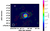 |
Fig. 1. Contours of the integrated CO (J = 3→2) (red contours) and HCO+ (J = 4→3) (green contours) emission over-plotted on the 350 GHz continuum image (pseudocolour). The levels for the contours are –4, –3, 3, 4, 5, and 6 times the rms of the CO (J = 3→2) moment 0 map (0.024 Jy/beam km/s) and –3, 3, 4, 5, 6, and 9 times the rms of the HCO+ (J = 4→3) moment 0 map (0.021 Jy/beam km/s). Dashed lines indicate negative contours. The negative features north and south of the AGN are caused by the short baselines missing in the imaging process. The beam size and shape (∼15.5×∼16.5 mas with a PA of –43°) for the two lines and the continuum are very similar, as marked by the ovals in red and cyan, respectively, in the lower left corner of the figure. |
2.2. Spectral line cubes
Before imaging, spectral line data were continuum-subtracted using line-free channels within each spectral window (CASA task uvcontsub). The five channels on either end of a spectral window were also excluded from the continuum subtraction. To reduce the data volume further, the continuum-subtracted data were time-averaged by 300 s.
The CO (J = 3→2) line cubes include significant emission from the 100 pc scale CND, especially the eastern knot, characterised by strong dust continuum and molecular line emission (García-Burillo et al. 2014)1. Therefore, for each line channel, we imaged a large, 9″ field around S1 and deconvolved using CLEAN (CASA task tclean). We used Briggs weighting with the “robust” parameter set to 2.0 (Briggs 1995) and 2.5 mas pixels. Initial line images showed a strong ripple pattern produced by undersampled, large-scale emission. We therefore flagged baselines shorter than 1200 kλ (structures larger than about 0 2) to reduce the ripple artefacts on the final line images.
We used the same approach for the images of HCO+ (J = 4→3). However, as there was no significant contribution from the CND, we imaged only the central 0 75. The integrated CO (J = 3→2) and HCO+ (J = 4→3) emissions are included in Fig. 1.
3. Spectral line analysis
To understand the kinematics of the gas close to the AGN, we analysed the central 250 mas (17.5 pc) by fitting a single Gaussian profile to the spectrum at each pixel of the line cubes. This approach provides a clearer representation of the velocity structure, as the more conventional moment maps yield representations that are harder to interpret due to the low S/N of the cubes. The Gaussian profile is expressed as
![Mathematical equation: $$ S_{\nu }(v) = A \exp {\left [-(v - v_0)^2/2s^2\right ]}, $$](/articles/aa/full_html/2025/07/aa53363-24/aa53363-24-eq8.gif) (1)
(1)
where Sν(v) is the observed flux density as a function of recessional velocity v, A is the line amplitude, v0 is the velocity at the line centre, and s is the linewidth (the standard deviation in the definition of the Gaussian function), which includes velocity dispersion but also contributions from rotation and radial motions within the beam. We constrained the fits in velocity to 900 km s−1<v0<1350 km s−1 resulting in fitted mean velocities of v0<300 km s−1. This was done to capture the main kinematic component near the AGN's systemic velocity. As a result, any high-velocity features outside this range, whether red-shifted or blue-shifted, were not accounted for in these fits. Additionally, we constrained the amplitudes to |A|>1.5×rms, where rms is the background noise of the line cubes, and the linewidths to 30 km s−1≤s≤190 km s−1. We rejected spectra for which the integrated S/N was less than 3. As a consequence, only fits in emission were kept. Further analysis of the central beam spectra and the PV diagrams reveal high-velocity absorption features at around v0∼400 km s−1. These trace a distinct physical process and are discussed separately in Sects. 4.4 and 4.3.
We performed a careful visual inspection of each of the spectral line fits in emission and conclude that the Gaussian model represents the line spectra well. However, in a small number of spectra closest to S1, where the lines are the broadest, we see evidence of multiple spectral peaks. This Gaussian fitting analysis effectively compresses the spectral line cubes into sky maps of parameters A, v0, and s. We used these cubes to further analyse the velocities, the linewidths, and the morphology of the emitting regions in Sects. 4.2 and 4.4.
4. Results
4.1. Integrated line emission
Figure 1 shows the integrated CO (J = 3→2) and HCO+ (J = 4→3) images as contours over the 365 GHz continuum image in pseudocolour. The continuum is dominated by a compact source with peak intensity at 8.3 mJy beam−1. In our ALMA image, the continuum peak is offset by ∼25 mas north-west of the VLBI position of S1. This is consistent with typical calibration errors in the ALMA calibration system (Gallimore et al. 2016). Perhaps the offset is real, but it seems unlikely. The integrated flux density of the continuum source is consistent with an extrapolation of the cm-wave flux densities, suggesting that the compact mm-wave continuum source is identically S1. We speculate that the offset might result from differences in the cm-wave and mm-wave structure of the phase reference, J0239–02. Moving forwards, we assume that the compact, 365 GHz continuum source coincides with the S1 VLBI continuum source and adjust the coordinates accordingly. We note that a similar position offset was observed in previous ALMA observations of the same galaxy (Gallimore et al. 2016), and more recently in the case of the Circinus galaxy (Tristram et al. 2022).
The integrated CO and the HCO+ images show a morphology roughly comparable to that found in previous ALMA observations (García-Burillo et al. 2016, 2019; Gallimore et al. 2016, with angular resolutions of 4, 5.9, and 2–6 pc, respectively). Any differences can be largely attributed to the application of our self-calibration procedure and the deliberate omission of the short baselines in our data analysis. The line emission resolves into two bright peaks bracketing the nuclear continuum source and oriented nearly east-west (PA 102°). The integrated line peaks are separated by roughly ∼30 mas (∼2 pc). North of the continuum source, marginally resolved line emission forms a bridge between the two emission line peaks, but there is a conspicuous gap south of the continuum source. Weak HCO+ emission is detected up to ∼50 mas (3.5 pc) from the nucleus, towards the north-west direction, and we also find weak HCO+ line absorption against the nucleus (See Fig. 1). The CO emission seems to extend towards the direction of the bright eastern knot, since there is a weak and smaller source, ∼65 mas (4.6 pc) to the southeastern direction (located at 2:42:40.7153 in RA and –0:00:47.9934 in Dec). While the morphology of the emission line sources is similar and follows the PA close to that of the central radio source S1 (104°) defined by Gallimore et al. (2004), their PAs differ from that of the H2O maser disc by ∼12° (see Fig. 3). Moreover, the HCO+ seems to come from a geometrically thicker disc, when comparing it to that of the CO. We also see that cutting the short baselines during our cleaning process created negative bowls in both line maps, ∼50 mas north and south from the AGN.
4.1.1. The CO (J = 3→2) to HCO+ (J = 4→3) line ratios
Figure 1 shows that the morphology of the compact molecular discs derived from the velocity-integrated line fluxes of the HCO+ (J = 4→3) and CO (J = 3→2) are approximately equal with some spatial variations. Figure 2 displays the line ratios quantitatively across the source and shows a systematic behaviour having a value of ∼1 near the main major axis of the molecular system (considering a PA of 114°), and decreasing to ∼0.5 above and below this axis. A prominent feature in this image is a strip with higher values ∼2 pc to the west of the AGN. It is interesting to note that this feature coincides with the low velocity region of the gas related to the drop to almost 0 km/s velocities in the west side of the disc (see Sect. 4.2 and Fig. 3). To enhance the areas with the colour scale, we limited the values displayed to a maximum of 2.0, nevertheless the few pixels that were left in blank in the middle of this strip reach higher values: in average the ratio of the lines in those pixels is 4. Viti et al. (2014) studied the entire CND of NGC 1068 in many molecular lines, covering a larger area, but at a lower spatial resolution than the data presented here. They defined four main regions in addition to the AGN: the CND regions, called eastern knot, western knot, CND-north, and CND-south. They found much higher values of the CO/HCO+ ratio than those found here, ranging from 9 to 16, and 11 at the AGN, all at a spatial resolution of 100 pc compared to the 1.1 pc resolution of the current data. They found the starburst ring (SB ring) to have a much higher line ratio of 72 at the resolution of 400 pc. We discuss the interpretation of these ratios further in Sect. 5.3.
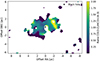 |
Fig. 2. Ratio of the integrated flux of CO (J = 3→2) to HCO+ (J = 4→3) as a function of position. Areas where the S/N of the CO line are <7 rms are suppressed. The central black star marks the position of the black hole. |
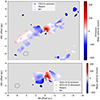 |
Fig. 3. Maps of CO and HCO+ recessional velocities in the nuclear region of NGC 1068. Velocities relative to systemic are shown in blue-red pseudocolour according to the colour bar at right. Top: CO (J = 3→2) emission velocities. Bottom: HCO+ (J = 4→3) emission and absorption velocities. In each plot, the ellipse in the lower left corner represents the beam size. North is up, and east is left. The black star marks the position of the supermassive black hole, and the small colourful dots represent the H2O megamaser disc (Gallimore et al. 2004). |
4.2. Recessional velocities and linewidths
We created velocity and linewidth maps derived from Gaussian fits to the cube spectra (Sect. 3). The results are shown in Figs. 3 and 4. It is important to note that the fit was done with the aim of representing the best kinematic system centred at the AGN, which resulted in Gaussians with mean velocities between –230 and 320 km/s. Therefore, any high-velocity component, either red-shifted or blue-shifted, is not represented in these plots. Recessional velocities are predominantly red-shifted (blue-shifted) immediately west (east) of S1, consistent with the sense of rotation of the water megamaser disc (Gallimore et al. 2004). The velocity pattern reverses beyond about 2 pc east and west of S1, consistent with the apparent counter-rotation reported by Impellizzeri et al. (2019) and Imanishi et al. (2020). However, there is also an extended region of blue-shifted CO emission extending to about 6 pc south-east of S1.
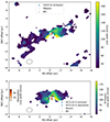 |
Fig. 4. Maps of CO and HCO+ linewidths s (Eq. (1)) in the nuclear region of NGC 1068. Emission linewidths are shown in blue-yellow pseudocolour according to the colour bar at right. Top: CO (J = 3→2) emission linewidths. Bottom: HCO+ (J = 4→3) emission and absorption linewidths (white-brown colour bar shown in the inset). In each plot, the ellipse in the lower left corner represents the beam size. North is up, and east is left. The black star marks the position of the supermassive black hole, and the small colourful dots represent the H2O megamaser disc (Gallimore et al. 2004). |
Not surprisingly, linewidths are highest near the central continuum source. In particular, there are wings of enhanced linewidth along the major axis of the H2O megamaser disc (Gallimore et al. 2004). The highest linewidths, approaching s = 200 km s−1, are found about 1 pc south-west of the radio continuum source. We further discuss this in Sect. 5.1. Beyond about 2–3 pc from S1, linewidths fall to s = 40−60 km s−1. There is also a region of low linewidth about 1 pc north-east of the nucleus. The velocities in this region tend to be slightly blue-shifted relative to systemic in both CO and HCO+.
Figure 5 shows the best-fit velocity centroids and linewidths as a function of distance from the S1 continuum source. Two results stand out. First, within about 1 pc of the central continuum source or S1, the red- and blue-shifted mean velocities in both lines (red dots for CO (J = 3→2) and green dots for HCO+ (J = 4→3)) are asymmetric with respect to the systemic velocity (marked by 0 in this plot). The mean velocities of the western red-shifted region (upper half) reach v0∼200 km s−1, but the eastern blue-shifted region (lower half) shows velocities typically below v0 = 100 km s−1. Second, beyond about 2 pc from S1, the mean velocities are typically within a linewidth of the systemic velocity, well below the rotation curve extrapolated from the H2O megamaser disc (dashed curves, cf. Impellizzeri et al. 2019; Gallimore & Impellizzeri 2023). Overall, the pattern suggests a switch in the molecular gas kinematics. Inside about 2 pc, the velocities are broadly consistent with rotation. Outside, however, the kinematics appear to be dominated by random motions, since the mean velocities are very low, of the order of 30 km/s on average. Nevertheless, the velocity dispersion remains constant with radius and of the order of 50 km/s.
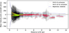 |
Fig. 5. Mean velocities obtained from the Gaussian fits to the CO (J = 3→2) (red) and HCO+ (J = 4→3) (green) emission, with bars representing best-fit linewidths (3×s, Eq. (1)), plotted against the distance to the central continuum source or S1. |
4.3. Spectra at the AGN position
Figure 1 shows absorption in the HCO+ (J = 4→3) at the position of the continuum peak. In the case of the CO (J = 3→2) line, there is a hole at the same position, and absorption is seen for the other line. The area marked by the dashed green contour has the shape of an ellipse, with its centre displaced with respect to the peak of the continuum by 1 or 2 pixels. This same region is characterised by the absence of emission of the CO (J = 3→2) transition. To analyse this in more detail, we extracted the spectra of both lines, using the CASA task viewer, integrated over one beam centred at the position of the AGN, that is, on top of the peak of the continuum (see Fig. 6). To our surprise, in the spectra of the CO (J = 3→2), we see several features in absorption as well. In this section, we characterise the profiles of both molecular transitions by fitting Gaussians to their spectra and calculating their significance.
 |
Fig. 6. Gaussian fits of the absorption and emission features of the CO (J = 3→2) and HCO+ (J = 4→3) spectra belonging to the central beam on top of the peak of the continuum relative to systemic velocity. The dotted line indicates –1 times the rms of the spectrum. For the systemic velocity, we used a value of 1130 km/s. |
In the case of the CO (J = 3→2) transition, we find high-velocity absorption centred at ∼411 km/s with a S/N of 3.5. The other possible absorption feature at ∼−637 km/s does not present a S/N high enough to be considered a real detection (see Fig. 6 top).
The HCO+ (J = 4→3) spectrum, in contrast, shows absorption centred at ∼−492 km/s with a S/N of 3.03, while the other possible absorption feature centred at ∼359 km/s does not present a S/N high enough to be considered a real detection (see Fig. 6 bottom). Both spectra present broad emission features at around +170 km/s that seem to be deformed by the absorption at high velocities, but it is only significant enough in the case of the CO (J = 3→2) line, with a S/N of 4.5. While the emission seems to peak at similar velocities with that of the HCN (J = 3→2) at 256 GHz found in Impellizzeri et al. (2019) (comparing to the raw spectrum), the strong nuclear absorption found in the same line differs significantly from our data. That is, their line profile is asymmetric: it peaks at systemic velocity, and it displays a blue wing extending to roughly –450 km/s. This HCN absorption was interpreted as a high-velocity nuclear molecular outflow. This feature is present neither in our HCO+ (J = 4→3) nor in our CO (J = 3→2) spectrum.
The 350 GHz continuum flux at the nuclear position is 8.3 mJy which is equivalent to a brightness temperature of Tc = 550 K. The negative fluxes in Fig. 6 near +400 km/s represent optical depths of ∼0.05 corresponding to a brightness temperature decrease of ΔTa∼−30 K. However, there is emission at adjacent velocities, and the major-axis PV diagrams (shown in Fig. 7) suggest that there is actually some emission in both lines at the nuclear position over most velocities between –400 and at least +400 km/s. Both the emission and absorption features seen in Fig. 6 are probably considerably broader than is apparent in the figure, but cancel each other at the velocities where they overlap. By interpolation from adjacent emission in Figs. 6 and 7, we estimate that in the absence of absorption, the actual line emission at the nuclear position near +400 km/s would be ∼0.5 mJy, and the actual absorption optical depths are more likely ∼0.1 in both lines.
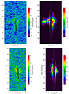 |
Fig. 7. Position-velocity diagram of the CO (J = 3→2) (top) and the HCO+ (J = 4→3) (bottom) along the major axis originated from the data (left) and the Gaussian fits (right). Black dots on the two top panels mark the positions of the H2O masers (Gallimore & Impellizzeri 2023). East is almost to the left, taking into account the PA used to make the diagram (PA = 114°). |
The physical conditions in the gas responsible for the absorption are discussed in Sect. 5.4.
4.4. Position-velocity diagrams
Figure 7 (left) shows the PV diagrams along the major axis of the CO (J = 3→2) and the HCO+ (J = 4→3) using a PA of 114°. We also plot in Fig. 7 (right) the analogue PV diagrams obtained from the Gaussian models. The diagrams for both lines are very similar. They show a lot of asymmetry between the west and east sides of the disc. While the west side has a large area with high intensities, the east side presents the peak intensity in a smaller area. The peaks are symmetric with radius, but not with velocity. Moreover, they differ in flux. The mean velocities decay quickly within the inner ∼2 pc on both sides of the disc. Nevertheless, the western side has a strong signal of apparent counter-rotation. This is, that there is signal in the quadrants of the PV diagrams where there should not be if we had a kinematic system rotating purely in one way. The linewidths are of the order of 200 km/s close to the nucleus and get abruptly reduced to around 50 km/s at r>2 pc. The Gaussian models are meant to only represent the emission, but it is clear that there are some areas with absorption features in the PV maps of the data (left). The missing emission at systemic velocity coinciding with the AGN stands out clearly in both lines, but the absorption at high velocity (at around 400 km/s) is very prominent in the CO (J = 3→2) map.
Figure 8 shows the PV diagrams along the minor axis of the CO (J = 3→2) (left) and the HCO+ (J = 4→3) using a PA of 24°. We also plot in Fig. 8 (right) the analogue PV diagrams obtained from the Gaussian models for the minor axis.
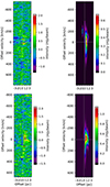 |
Fig. 8. Position-velocity diagram of the CO (J = 3→2) (top) and the HCO+ (J = 4→3) (bottom) along the minor axis from the data (left) and the Gaussian fits (right). North is almost to the right taking into account the PA used to make the diagram (PA = 24°). |
5. Discussion
Here we consider further two issues that became evident in exploring the data that are difficult to explain in the context of gravitationally bound, rotating disc models, namely:
-
The very low observed velocities compared to the predictions of Keplerian rotation around the central black hole.
-
The east-west asymmetries in the PV diagrams very close to the active nucleus.
For this, we first show that the large linewidth values can arise from a beam smearing effect with the help of the tool 3DBarolo (Di Teodoro & Fraternali 2015), and then we test the possibility of having asymmetric drift assuming that beam smearing is not causing the large velocity dispersions.
5.1. Line broadening
The high linewidths and low rotational speeds observed suggest that the molecular gas might be highly turbulent within the central ∼2 pc. On the other hand, the 16 mas (1.1 pc) beam does not resolve the molecular disc traced by H2O megamaser emission. As rotational speeds reach ∼330 km s−1 in the maser disc, the beam-averaged linewidth is expected to be large. We therefore used 3DBarolo (Di Teodoro & Fraternali 2015) to simulate an ALMA observation of the H2O megamaser disc and assess the contribution of rotational kinematics to the observed linewidth. The software package 3DBarolo allows for modelling the rotation curves and other parameters of the disc. It uses a tilted ring model, which consists of nested rings with constant circular velocities each allowing for peculiar morphologies as warped or lopsided systems, and considers beam smearing effects by adding a convolution step before providing the final model. We set up the simulation using the observed rotation curve and orientation of the H2O megamaser disc (Gallimore & Impellizzeri 2023). The parameters are summarised in Table 1. As H2O masers necessarily trace hotter and denser molecular gas, we chose a larger outer radius (40 mas = 2.8 pc) than the observed megamaser disc to simulate possible emission from CO or HCO+. We also assumed a velocity dispersion σ = 15 km s−1, roughly two channels, to ensure Nyquist sampling of the simulated spectra. The true velocity dispersion of the maser disc might be smaller, but this simulated dispersion is much less than the range of rotation speeds averaged over the beam and has little impact on the results. The ring width, δr = 2 mas, was chosen as a compromise between finely sampling the Keplerian rotation curve near the inner radius and computation speed. In sum, the simulation involved 17 nested rings between 5 and 40 mas radius. This setup has the implicit assumption that the kinematics defined by the H2O masers extend towards larger radii.
3DBarolo simulation parameters.
We performed two simulations, changing only the emissivity profile of the rings. In Model 1, the emissivity is constant as a function of radius, and in Model 2, the emissivity law falls as r−2. Models were calculated on 0.5 mas pixel grids (i.e. 5× narrower pixels than used for the ALMA data). The objective of using smaller pixels is to capture the whole range of velocities observed in the masers, especially the highest velocities closer to the BH that would help create broader lines by beam smearing. The resulting model cubes were then convolved with the ALMA beam (16.3×15.1 mas, PA −45°). Finally, we repeated the Gaussian fitting analysis for the simulated cubes (see Sect. 3).
Figure 9 compares the integrated intensity, velocity field, and linewidths of the 3DBarolo simulations and our ALMA observations of HCO+ (J = 4→3). We note that the images have been rotated by 24° for comparison. It is difficult to compare the integrated intensity images because 3DBarolo does not simulate absorption. Even so, the distribution of molecular gas is clearly more complex than our necessarily simplified 3DBarolo simulations. The simulated velocity field only broadly resembles that observed within the inner pc. Again, absorption challenges the comparison: only in the region immediately surrounding the central continuum source do we see rotation speeds comparable to the simulation. Possibly, the molecular accretion disc does not extend far beyond the region sampled by H2O masers.
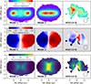 |
Fig. 9. Intensities at the mean velocities (top row), mean velocities (middle row), and linewidths (bottom row) obtained from the Gaussian fit for Model 1 (left column), Model 2 (middle column), and the HCO+ (J = 4→3) (right column). For all figures: The ellipse in the right panel represents the size of the beam for the observations, which we used to convolve the images of the models. The colour bar on top of the left panel applies to the three sub-images. The coordinate system is rotated by 24° (see details in text). |
The linewidth simulations are more informative. In the simulations, the linewidths form a butterfly-shaped pattern within the central 2 pc. In Model 2, where the emissivity profile is more centrally concentrated, the linewidths are comparable to those observed in CO (J = 3→2) and HCO+ (J = 4→3). We conclude that the observed high linewidths in the central 2 pc could be the result of beam smearing and plausibly trace unresolved rotation in the H2O maser disc rather than turbulent motions.
5.2. Asymmetric drift and sub-Keplerian rotation
The relatively high values of σ/v seen in both the models and observations suggest another explanation for the apparent observed sub-Keplerian rotation velocities, namely ’asymmetric drift’. This is the phenomenon in axisymmetric systems, also seen in our Galaxy (Binney & Tremaine 2008), where the mean tangential velocity, vt, is lower than the circular velocity, vc, if the velocity dispersions are high and gradients in density or dispersion exist. The underlying cause is that–in the presence of radial dispersion–at any radius we observe, we also see clouds whose mean radius is smaller than the observed radius. Through the conservation of angular momentum, these clouds have tangential velocities lower than the circular velocities at this point. This possibility was also noted by Vollmer et al. (2022). The behaviour is captured in the axisymmetric Jeans Equation, given by
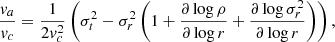
where va≡<vt>−vc is the asymmetric drift; σt, σr are the tangential and radial velocity dispersions; and ρ is the cloud density. All the quantities are potentially functions of r. The observations suggest that, at least at some radii σ/vc∼1 and varies radially.
In the central region, 1<r<2 pc, we can estimate roughly from the observed moment maps (Figs. 3 and 4) that σ∼vc∼100 km/s,  , and we assume
  . For isotropic turbulence (σt≡σr≡σ), this yields va/vc∼0.5, in which case the observed velocity would be about half the actual Keplerian circular velocity. In Sect. 5.1 we point out that for highly centrally concentrated gas distributions (
 ), the beam smearing at the ALMA resolution causes an overestimation of σ in the central region. However in this case, the larger value of the second-to-last term in the Jeans Equation compensates for the smaller value of the last term and leads to a similar estimate of
  .
.
In the outer 2–4 pc region, the situation differs. σ is approximately constant at ∼50 km/s, while ∂log ρ/∂log r∼−1 and vc∼140 km/s. As a result, the Jeans equation predicts 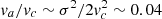 , which is negligible. The measured rotational velocities in these two regions are ∼90 km/s and <10 km/s, respectively. Hence the asymmetric drift can be considered a plausible explanation for the sub-Keplerian rotation in the inner region, but not at radii
  3 pc. The very low velocities at the latter projected positions cannot maintain the gas against the gravitational force of the central black hole. They may be transient, or at much larger radii but seen in projection closer to the nucleus, or supported by another mechanism, such as radiation pressure.
Vollmer et al. (2022) present a numerical model of a dense cloud falling onto a pre-existing disc at the centre of NGC 1068, based on detailed assumptions on the physical processes in the parsec scale region. Their basic physical picture is quite similar to that presented here (discussed in Sects. 5.4 and 5.5 of this work) and fits the earlier, lower spatial resolution ALMA data reasonably well. Here, however, we limit our analysis to quantities that can be derived fairly directly from the observed data, without additional assumptions about the dynamic processes.
5.3. CO to HCO+ line ratios
In Sect. 4.1.1 we pointed out that the CO (J = 3→2) to HCO+ (J = 4→3) line ratios in the parsec-sized region around the nucleus are in the range 0.5–2, which is a factor of 10–20 lower than that seen in the CND and also around the AGN when measured at much lower spatial resolution.
Vollmer et al. (2022) presents molecular line images of the same transitions of other ALMA observations of NGC 1068. These show similar low ratios of the same lines and transitions as ours at a slightly lower spatial resolution. From their Table 4, we obtain an integrated intensity ratio of CO to HCO+ of 1.8 in lower-resolution observations of the torus region. Vollmer et al. (2022) did not comment explicitly on the ratios. Nevertheless, this value is consistent with the detailed physical and dynamical model presented in the same work within a factor of two or three (see also Sect. 4.3 below).
García-Burillo et al. (2021) compiled line ratios for a large sample of AGNs measured at the AGN position. These are rather small, ranging from ∼2.8 to 5.7 (for what they refer to as the GATOS sample), and was interpreted as pointing at the presence of high-density molecular gas at small radii inside the central ∼3 to 10 pc. In comparison, another sample of AGNs, the NUGA sample (Combes et al. 2019; Audibert et al. 2019), shows higher values for the ratios of ∼8.5 to 38. An important difference between these two samples is that the latter have lower luminosity and Eddington ratios. The highest ratios around 30 were interpreted as an indication of the molecular torus having the lowest gas density. Nevertheless, outflows might explain the observations of the GATOS sample by preferentially removing diffuse, lower-density molecular gas while leaving heavier and higher-density clumps behind.
The difference by an order of magnitude in this line ratio was further interpreted as evidence of radial density stratification of the molecular tori (García-Burillo et al. 2021). Therefore, a drop in this ratio as one approaches the nucleus seems to be a more general trend in AGNs.
In the diffuse interstellar medium in our Galaxy, the CO (J = 1→0)/HCO+ (J = 1→0) ratio is typically ∼100 (Liszt & Gerin 2023), much higher than the ratio for these lines in the circumnuclear regions of AGNs (e.g. Viti et al. 2014).
This decrease in the CO/HCO+ ratio near AGNs is usually attributed to higher densities (García-Burillo et al. 2021), because the critical density of the HCO+ line (∼2×106 cm−3) is much higher than that of CO (∼8000 cm−3). The critical density is that where collisional de-excitation of the upper state of a molecular transition competes with spontaneous radiative de-excitation; further density increases no longer cause increases in the molecular emission. However, the calculations in Viti et al. (2014) (Table 12) indicate that the density in the more extended regions around the nucleus of NGC 1068 is already ∼106 cm−3, that is, at the HCO+ critical density. Thus, further density increases would not decrease the CO/HCO+ ratio to the values we measure. In any case, the maximum line ratio shift between low and high-density environments would be the ratio of the critical densities of the two molecules, in this case ∼120. Hence our observed minimum line ratio of ∼0.5 is at the extreme edge of what can be explained by density effects, suggesting that a chemical shift in the abundance ratio of CO to HCO+ also plays a role.
Kohno (2005) attributed drops in the CO/HCN line ratio near AGNs to the intense X-ray environment near the nucleus. Izumi et al. (2013) and Martín et al. (2021) however claim that the low value of this ratio is more likely the result of high-temperature-induced chemical shifts near AGNs than X-ray or cosmic ray radiation. The same mechanisms may be responsible for the decrease in the CO/HCO+ ratio from CND towards the AGN seen here. If future higher-resolution observations show that this ratio continues to drop closer to the nucleus, then mechanisms other than density increases must be involved.
5.4. Near-nuclear motions and possible filamentary structures
In Sect. 4.3 we indicated the existence of a highly red-shifted absorption feature seen as a dark blue region in Fig. 7 at velocities of +350 to +500 km/s at the continuum peak position. The feature seems to be contiguous with emission to the west of the nucleus at velocities of –50 to +300 km/s. The continuity in space and velocity suggests that this is one structure changing from emission to absorption as it passes in front of the AGN continuum. If the continuum source were in fact point-like, this would indicate a non-circular, infalling cloud or filament, since material in circular motion would have the systemic velocity when seen in front of the source. However, Impellizzeri et al. (2019) show that the brightest nuclear continuum emission is extended approximately 1.0 parsec, mostly along the major axis of our molecular emission. The red-shifted absorption could in principle arise from circularly moving gas on the west side of the source, unresolved within our ALMA beam.
However, several arguments can be made against a simple model of a ring of molecular gas orbiting at a radius of ∼0.5 parsec: (1) The major-axis PV diagram (see Fig. 7) is strongly asymmetric at velocities |V−Vsys|>100 km/s. (2) When the ring crosses in front of the centre of the continuum source, it should cause a deep absorption at systemic velocity. In the data, only a weak absorption is seen at this velocity. (3) In a complete circular ring orbiting the continuum emitter, the highest velocity should be seen in emission at the tangent point where the gas is moving directly away from the viewer, rather than absorption in front of the continuum source, where the velocity is diminished by the cosine of the angle to the line of sight.
These arguments suggest that the high-velocity, red-shifted feature seen in both emission and absorption represents an incomplete ring or filament primarily on the west side of the nucleus. This material may also represent a filament or sheared cloud of gas on a highly elliptical or parabolic orbit. In either case, its motion would cause changes in appearance and velocity on timescales of ∼r/v∼103 years. We note that Müller Sánchez et al. (2009) found a red-shifted infalling filament or ‘tongue’ of molecular hydrogen from the east on larger scales and lower velocities. Also, García-Burillo et al. (2019) note a large low-surface-brightness, low-velocity connection east of the nucleus to the CND.
It is clear that the scenario of an infalling cloud connects with neither the interpretation of the outflow in HCN (Impellizzeri et al. 2019) nor with the inferred outflow at larger scales (CND scales, García-Burillo et al. 2014) seen in several other molecular lines (CO(3-2), CO(6-5), HCN(4-3), and HCO+(4-3)). Nevertheless, these pictures are not mutually exclusive. The most intriguing puzzle is why we do not see deep absorption at systemic velocity as in the HCN (Impellizzeri et al. 2019). However, the molecules CO and HCO+ and the HCN do not have a common chemical path. Therefore they are not expected to behave in the same way.
Whatever the kinematic origin of the molecular gas, the proximate appearance of absorption and emission in the nuclear spectra allows estimates of the physical conditions in the cloud. In Sect. 4.3 we estimated the peak continuum brightness temperature to be Tc∼550 K and the depth of the absorption feature to be ΔTa∼−30 K, while the off-nuclear line emission brightness fluxes are ∼0.5−1.0 mJy corresponding to brightness temperatures of Tem∼30−60 K. For gas with an excitation temperature of Tx, these quantities are related by
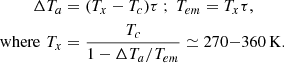
The HCO+ profile yields similar values. These are relatively high temperatures for molecular clouds but are similar to the dust temperatures found on similar scales in Gámez Rosas et al. (2022). They may also indicate that the excitation temperature is influenced by the intense radiation field near the AGN. If we nonetheless make the assumption of LTE, we can compute the column densities of the molecules. The absorption profiles in Fig. 6 have numerically integrated optical depths, ∫τdv, of 20 km/s and 10 km/s for the CO (J = 3→2) and HCO+ (J = 4→3) transitions, respectively. From LTE calculations at Tx = 300 K, the total column densities in the two molecules are NCO∼5×1018 cm−2 and  . For an abundance ratio
  similar to that found in diffuse molecular gas in our Galaxy (Liszt & Gerin 2023), the latter column density implies
  cm−2. However, as discussed in Sect. 5.3, the abundances of HCO+ may be enhanced in the high ionisation environment of the AGN, which would lower the estimated hydrogen column density. An independent lower limit to the column density of an orbiting, dusty molecular cloud can be made from a ‘dusty Eddington’ calculation of the balance between radiation pressure and gravity. If all of the AGN's UV radiation is absorbed by the dust at the cloud's exposed face, the outwards radiation force per unit area is LUV/4πcr2, while the inward gravitational force per unit area of the overlying column of gas is GMAGNmHNH/r2. Taking the estimates of the mass and bolometric luminosity of NGC 1068 used in GRAVITY Collaboration (2020), a cloud can only be in a stable or infalling orbit if NH∼1×1024 cm−2 or greater. This suggests that the HCO+ abundance in NGC 1068 is similar to the diffuse Galactic value. In this case the high values of the HCO+/CO line ratios discussed in Sect. 4.1.1 indicate a deficiency of CO rather than a surplus of HCO+, and the effect of the high ionisation environment near the AGN would be to destroy CO by conversion to C+.
5.5. Kinematic modelling of the high-velocity feature
The absorption feature seen at velocities vlos of up to 500 km/s must be an infalling cloud near the nucleus. This velocity should be compared to the estimate of the Keplerian circular velocity at 10 mas radius (0.7 pc) of 315 km/s in Gallimore & Impellizzeri (2023) based on water maser kinematics. In a Keplerian gravitational field, this corresponds to a velocity of free fall from infinity of 445 km/s. Thus measuring vlos∼500 km/s implies that the gas must be closer than 8 mas (0.5 pc) to the black hole. This is consistent with it being within the ALMA beam at the nuclear position (FWHP ∼ 15 mas) and the fact that it must be in front of the nuclear continuum source (radius ∼10 mas from Gallimore & Impellizzeri 2023). This radius estimate is similar to the size of the torus seen in the infrared (Gámez Rosas et al. 2022), and the absorbing cloud is probably related to that structure.
We attempted to model the kinematics of the western, high-velocity, red-shifted emission and absorption features as an extended filament falling in from infinity on a parabolic orbit. For simplicity we assumed that the pole of the orbit lies in the plane of the sky. In reality the orbit of the filament must be somewhat inclined with respect to that of the torus in order to avoid a collision between the two structures. With these assumptions there are two parameters that define an orbit: the angle of the symmetry axis of the parabola from the line of sight and the distance of closest approach to the black hole (the peritrypa, where mavri trypa is Greek for ‘black hole’). The model orbits were chosen to reproduce the main features of the observed filament in the major-axis PV diagram (Fig. 7): namely, a continuous feature approaching the nucleus from the west seen in emission at velocities of +80 to +300 km/s that turns into absorption at +300 to +500 km/s and is not seen as a blue-shifted feature to the east of the nucleus. We ignored features within 80 km/s of systemic in the modelling because these are confused with features arising from the molecular disc at larger radii. We only modelled the kinematics of the infalling material and the relative roles of absorption and emission as it passes in front of the central continuum source. We did not include any detailed physics about the filament such as changes in temperature, density, or ionisation as it approaches the centre.
Figure 10 shows the trajectories in the plane of the orbits and simulated PV diagrams for a string of clouds along three model orbits; and Fig. 11 shows a 3D rendering of the first model to aid visualisation. Figure 10 (left) shows a model where the axis of the orbit is along the line of sight and peritrypa = 0.1 pc; (centre) a model where it is perpendicular to the line of sight and peritrypa = 0.5 pc; and (right) a similar to that presented in the middle panel but with the initial part of the orbit truncated. Comments on these three models include the following: The first model (left panel) matches the emission and absorption structure of Fig. 7. It was necessary to terminate the orbit at closest approach in order to eliminate the appearance of a similar blue-shifted eastern feature. This termination could be explained by the destruction of the clouds near the black hole by radiation near the central source. To reproduce the maximum observed velocity, ∼500 km/s, the distance of closest approach must be quite small, 0.1 pc, because most of the velocity at this point is projected perpendicular to the line of sight. This model requires the continuum source to be extended so that some of the filamentary clouds are seen in absorption before they pass around the back of the black hole. In fact, this source has a radius of ∼0.7 pc (Gallimore & Impellizzeri 2023), larger than the orbital peritrypa distance. The second model (middle panel) shows an orbit approaching from the west, passing 0.4 pc from the centre while moving directly away from the observer and leaving again towards the west. The peritrypa distance is larger because the total velocity at this point is along the line of sight, and the velocity is red-shifted along the entire orbit, so there is no problem eliminating an eastern blue-shifted component. There is excess absorption at relatively low velocities relative to the observed PV diagram because the clouds are seen in front of the continuum source for a relatively long path when they are at larger radii and moving across the line of sight. In this model, the actual size of the continuum source is not important. In the third model (right panel), the excess absorption in the second model can be suppressed by clipping the piece of the orbit in front of the continuum source. This change improves the kinematic match to the observed PV diagram but, of course, leaves unanswered the problem of why we do not see the initial infalling segment of the orbit.
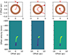 |
Fig. 10. Parabolic trajectories of a filament of clouds approaching the peritrypa in three simulations. The top drawings illustrate the orbits in the plane of the filament, while the bottom series illustrate synthetic PV diagrams derived from the system of filament plus continuum source that can be compared with the actual observations in Fig. 7. In each case, the observer views the system from the top (red ‘V’ mark). The orange bar indicates the continuum source; clouds in front of this from the observer's point of view are seen in absorption, otherwise in emission. The red dot indicates where the orbit enters the field of view. The brown circle at 3 pc radius indicates the typical radius of the molecular disc described in this paper. To avoid a collision between the disc and the orbital plane of the filament, the latter must be somewhat inclined with respect to that of the disc. The 3D rendering of the first model is shown in Fig. 11, which illustrates the relative orientations of the disc, filament, continuum source, and observer for this case. The three models are: (left panel) a trajectory seen along the parabolic axis, in which the distance of closest approach is 0.1 pc (see text) and the orbit is truncated at this point; (middle panel) the parabolic axis is perpendicular to the line of sight; and (right panel) same as in the middle panel, but the filament only begins just before peritrypa. Velocities within ±80 km/s of systemic are suppressed. The synthetic PV distributions are convolved with a Gaussian of 0.5 pc in the spatial direction to simulate the ALMA resolution. |
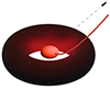 |
Fig. 11. 3D rendering showing the spatial relationships of the components for the first case in Fig. 10 (left), the observer's line of sight from the back of the illustration, and the inclination of the disc plane and the filament's orbital plane. Illustration: W. Westerik. |
The larger radius of ∼0.4 pc is similar to that of the main infrared dust structure. A radius of ∼0.1 pc would put the molecular clouds in the filament at or within the 'sublimation radius’ where the UV radiation from the central engine destroys the dust. This radius was estimated by GRAVITY Collaboration (2020) to be in the range 0.08–0.27 pc, depending on the assumed total UV luminosity of NGC 1068. In all three cases, the peritrypa radius is within the estimated radius of the continuum emitting source (Gallimore et al. 1996a), but we do not further explore the consequences of this proximity here.
6. Conclusions
We present high spatial and spectral resolution ALMA observations of the HCO+ (J = 4→3) and CO (J = 3→2) lines in the near-nuclear region of the prototype Seyfert 2 galaxy NGC 1068 and its underlying continuum. We present the results as moment maps, PV diagrams, and spectra at the position of the nuclear continuum source. We made a simple kinematic model with the help of the 3DBarolo software, and we analysed the possibility of explaining the non-Keplerian motions with asymmetric drift. We discussed the absorption feature seen in both lines on top of the AGN and presented a simple model for a cloud in an elliptical orbit. We also noticed the very low line intensity ratio of the CO to the HCO+.
We arrive at the following conclusions:
-
The line emitting regions traced by CO and HCO+ (see Fig. 1) present significant asymmetry in morphologies, mean velocities, surface brightness, and linewidths, when comparing the east and west sides of the disc. We find this suggests a highly disturbed kinematic system. Such traces can be a consequence of possible past events (e.g. mergers) or ongoing processes (accretion or jet interactions).
-
In the inner regions (radius ≤ 2 pc) the sub-Keplerian rotation can be explained by asymmetric drift associated with high velocity dispersions. This is crucial for understanding the stability and longevity of the molecular structures around the AGN. Nevertheless, the very low velocity components at larger radii (r ≥ 3 pc) cannot be explained this way, and radiation pressure may also be important to support the gas. In particular, on the east side, the CO (J = 3→2) emission seems to extend out to ∼13 pc, from radii of ∼4 pc. This is most probably a filament connecting the torus to the CND.
-
The gas very close to the AGN shows very broad linewidths that may indicate high turbulent velocities. A simple kinematic model indicates that the broad lines seen in the inner ≤2 pc can also be accounted for beam smearing of the Keplerian disc associated with the H2O masers with a high central density.
-
The molecular gas near the central continuum source or S1, observed in both, emission–at approximately 300 km/s – and red-shifted absorption – at around 400 km/s–, suggests the presence of dynamic and possibly transient structures, such as a partial ring, a filament, or sheared gas clouds on elliptical or parabolic orbits. These features exhibit high-excitation temperatures around 300 K and significant column densities (e.g. NCO≈5×1018 cm−2,
 ). The high velocity of the absorption component places it at or within the infrared dusty structure at 0.5 pc from the central engine, while some of the kinematic models place it much closer, ∼0.1 pc, near the sublimation radius of the dust, suggesting that they are intimately connected to the central engine, possibly marking the innermost regions of AGN feeding channels where extreme physical processes are at play.
 -
The observed CO/HCO+ line ratios in NGC 1068 are notably lower than typically seen in other AGNs, and there is a clear trend towards lower ratios with increasing spatial resolution. This pattern likely reflects the proximity of the gas to the AGN, where intense X-ray and cosmic ray emissions from the central engine drive the chemical conversion of CO into CI or CII. This transformation reduces CO abundances in regions illuminated directly by the AGN, suggesting a direct influence of the AGN's radiation on the surrounding molecular gas chemistry.
The high resolution ALMA data presented here reveal highly asymmetric and dynamic molecular gas structures–including inflows and turbulent motions–that must play crucial roles in both fuelling the AGN and in the feedback processes that regulate the host galaxy's evolution.
Acknowledgments
This paper makes use of the following ALMA data: ADS/JAO.ALMA#2019.1.01540.S. ALMA is a partnership of ESO (representing its member states), NSF (USA) and NINS (Japan), together with NRC (Canada), NSTC and ASIAA (Taiwan), and KASI (Republic of Korea), in cooperation with the Republic of Chile. The Joint ALMA Observatory is operated by ESO, AUI/NRAO and NAOJ. SGB acknowledges support from the Spanish grant PID2022-138560NB-I00, funded by MCIN/AEI/10.13039/501100011033/FEDER, EU. IM acknowledges financial support from the Severo Ochoa grant CEX2021-001131-S funded by MCIN/AEI/10.13039/501100011033, and the Spanish MCIU grant PID2022-140871NB-C21. CRA acknowledges support from the Agencia Estatal de Investigación of the Ministerio de Ciencia, Innovación y Universidades (MCIU/AEI) under the grant “Tracking active galactic nuclei feedback from parsec to kiloparsec scales”, with reference PID2022-141105NB-I00 and the European Regional Development Fund (ERDF). AF thanks project PID2022-137980NB-I00 funded by the Spanish Ministry of Science and Innovation/State Agency of Research MCIN/AEI/10.13039/501100011033 and by “ERDF A way of making Europe”. The PI acknowledges assistance from Allegro, the European ALMA Regional Center node in the Netherlands. We thank Ed Formalont for valuable advice on the imaging process of the data. The authors thank Willem Westerik for providing graphic support for Fig. 11.
This area was first defined in Viti et al. (2014) (see Fig. 1) and has continued to be used in subsequent studies, such as García-Burillo et al. (2016, 2019).
References
- Alonso-Herrero, A., Pereira-Santaella, M., García-Burillo, S., et al. 2018, ApJ, 859, 144 [Google Scholar]
- Alonso-Herrero, A., García-Burillo, S., Pereira-Santaella, M., et al. 2019, A&A, 628, A65 [NASA ADS] [CrossRef] [EDP Sciences] [Google Scholar]
- Antonucci, R. 1993, ARA&A, 31, 473 [Google Scholar]
- Antonucci, R. R. J., & Miller, J. S. 1985, ApJ, 297, 621 [NASA ADS] [CrossRef] [Google Scholar]
- Audibert, A., Combes, F., García-Burillo, S., et al. 2019, A&A, 632, A33 [NASA ADS] [CrossRef] [EDP Sciences] [Google Scholar]
- Bannikova, E. Y., Akerman, N. O., Capaccioli, M., et al. 2023, MNRAS, 518, 742 [Google Scholar]
- Binney, J., & Tremaine, S. 2008, Galactic Dynamics: Second Edition (Princeton, NJ USA: Princeton University Press) [Google Scholar]
- Briggs, D. S. 1995, Ph.D. Thesis (New Mexico Institute of Mining and Technology), USA [Google Scholar]
- Capetti, A., Macchetto, F., Axon, D. J., Sparks, W. B., & Boksenberg, A. 1995, ApJ, 452, L87 [CrossRef] [Google Scholar]
- CASA Team, Bean, B., Bhatnagar, S., et al. 2022, PASP, 134, 114501 [NASA ADS] [CrossRef] [Google Scholar]
- Chan, C. -H., & Krolik, J. H. 2016, ApJ, 825, 67 [NASA ADS] [CrossRef] [Google Scholar]
- Chan, C. -H., & Krolik, J. H. 2017, ApJ, 843, 58 [NASA ADS] [CrossRef] [Google Scholar]
- Combes, F., García-Burillo, S., Audibert, A., et al. 2019, A&A, 623, A79 [NASA ADS] [CrossRef] [EDP Sciences] [Google Scholar]
- Cornwell, T. J., & Wilkinson, P. N. 1981, MNRAS, 196, 1067 [NASA ADS] [Google Scholar]
- Di Teodoro, E. M., & Fraternali, F. 2015, MNRAS, 451, 3021 [Google Scholar]
- Dorodnitsyn, A., Kallman, T., & Proga, D. 2008, ApJ, 675, L5 [Google Scholar]
- Dorodnitsyn, A., Bisnovatyi-Kogan, G. S., & Kallman, T. 2011, ApJ, 741, 29 [Google Scholar]
- Elitzur, M., & Shlosman, I. 2006, ApJ, 648, L101 [Google Scholar]
- Emmering, R. T., Blandford, R. D., & Shlosman, I. 1992, ApJ, 385, 460 [NASA ADS] [CrossRef] [Google Scholar]
- Gallimore, J. F., & Impellizzeri, C. M. V. 2023, ApJ, 951, 109 [NASA ADS] [CrossRef] [Google Scholar]
- Gallimore, J. F., Baum, S. A., & O’Dea, C. P. 1996a, ApJ, 464, 198 [NASA ADS] [CrossRef] [Google Scholar]
- Gallimore, J. F., Baum, S. A., O’Dea, C. P., Brinks, E., & Pedlar, A. 1996b, ApJ, 462, 740 [Google Scholar]
- Gallimore, J. F., Baum, S. A., & O’Dea, C. P. 1997, Nature, 388, 852 [Google Scholar]
- Gallimore, J. F., Henkel, C., Baum, S. A., et al. 2001, ApJ, 556, 694 [Google Scholar]
- Gallimore, J. F., Baum, S. A., & O’Dea, C. P. 2004, ApJ, 613, 794 [Google Scholar]
- Gallimore, J. F., Elitzur, M., Maiolino, R., et al. 2016, ApJ, 829, L7 [Google Scholar]
- Gámez Rosas, V., Isbell, J. W., Jaffe, W., et al. 2022, Nature, 602, 403 [CrossRef] [Google Scholar]
- García-Burillo, S., Combes, F., Usero, A., et al. 2014, A&A, 567, A125 [Google Scholar]
- García-Burillo, S., Combes, F., Ramos Almeida, C., et al. 2016, ApJ, 823, L12 [Google Scholar]
- García-Burillo, S., Combes, F., Ramos Almeida, C., et al. 2019, A&A, 632, A61 [Google Scholar]
- García-Burillo, S., Alonso-Herrero, A., Ramos Almeida, C., et al. 2021, A&A, 652, A98 [NASA ADS] [CrossRef] [Google Scholar]
- GRAVITY Collaboration (Pfuhl, O., et al.) 2020, A&A, 634, A1 [NASA ADS] [CrossRef] [EDP Sciences] [Google Scholar]
- Greenhill, L. J., & Gwinn, C. R. 1997, Ap&SS, 248, 261 [Google Scholar]
- Imanishi, M., Nakanishi, K., & Izumi, T. 2016, ApJ, 822, L10 [Google Scholar]
- Imanishi, M., Nakanishi, K., Izumi, T., & Wada, K. 2018, ApJ, 853, L25 [NASA ADS] [CrossRef] [Google Scholar]
- Imanishi, M., Nguyen, D. D., Wada, K., et al. 2020, ApJ, 902, 99 [CrossRef] [Google Scholar]
- Impellizzeri, C. M. V., Gallimore, J. F., Baum, S. A., et al. 2019, ApJ, 884, L28 [NASA ADS] [CrossRef] [Google Scholar]
- Izumi, T., Kohno, K., Martín, S., et al. 2013, PASJ, 65, 100 [NASA ADS] [Google Scholar]
- Khim, H., & Yi, S. K. 2017, ApJ, 846, 155 [Google Scholar]
- Kishimoto, M. 1999, ApJ, 518, 676 [NASA ADS] [CrossRef] [Google Scholar]
- Kohno, K. 2005, in The Evolution of Starbursts, eds. S. Hüttmeister, E. Manthey, D. Bomans, & K. Weis, American Institute of Physics Conference Series, 783, 203 [Google Scholar]
- Konigl, A., & Kartje, J. F. 1994, ApJ, 434, 446 [NASA ADS] [CrossRef] [Google Scholar]
- Krolik, J. H. 2007, ApJ, 661, 52 [NASA ADS] [CrossRef] [Google Scholar]
- Krolik, J. H., & Begelman, M. C. 1986, ApJ, 308, L55 [CrossRef] [Google Scholar]
- Krolik, J. H., & Begelman, M. C. 1988, ApJ, 329, 702 [Google Scholar]
- Liszt, H., & Gerin, M. 2023, ApJ, 943, 172 [NASA ADS] [CrossRef] [Google Scholar]
- Martín, S., Mangum, J. G., Harada, N., et al. 2021, A&A, 656, A46 [NASA ADS] [CrossRef] [EDP Sciences] [Google Scholar]
- Matt, G., Bianchi, S., Guainazzi, M., & Molendi, S. 2004, A&A, 414, 155 [NASA ADS] [CrossRef] [EDP Sciences] [Google Scholar]
- Miller, J. S., & Goodrich, R. W. 1990, ApJ, 355, 456 [NASA ADS] [CrossRef] [Google Scholar]
- Moran, E. C., Barth, A. J., Kay, L. E., & Filippenko, A. V. 2000, ApJ, 540, L73 [NASA ADS] [CrossRef] [Google Scholar]
- Müller Sánchez, F., Davies, R. I., Genzel, R., et al. 2009, ApJ, 691, 749 [Google Scholar]
- Muxlow, T. W. B., Pedlar, A., Holloway, A. J., Gallimore, J. F., & Antonucci, R. R. J. 1996, MNRAS, 278, 854 [NASA ADS] [CrossRef] [Google Scholar]
- Pier, E. A., & Voit, G. M. 1995, ApJ, 450, 628 [NASA ADS] [CrossRef] [Google Scholar]
- Ramos Almeida, C., Martínez González, M. J., Asensio Ramos, A., et al. 2016, MNRAS, 461, 1387 [NASA ADS] [CrossRef] [Google Scholar]
- Schwab, F. R. 1980, in 1980 Intl Optical Computing Conf I, ed. W. T. Rhodes (International Society for Optics and Photonics (SPIE)), 0231, 18 [Google Scholar]
- Simpson, C. 2005, MNRAS, 360, 565 [NASA ADS] [CrossRef] [Google Scholar]
- Tran, H. D. 1995, ApJ, 440, 565 [NASA ADS] [CrossRef] [Google Scholar]
- Tran, H. D., Miller, J. S., & Kay, L. E. 1992, ApJ, 397, 452 [NASA ADS] [CrossRef] [Google Scholar]
- Tristram, K. R. W., Impellizzeri, C. M. V., Zhang, Z. -Y., et al. 2022, A&A, 664, A142 [NASA ADS] [CrossRef] [EDP Sciences] [Google Scholar]
- Urry, C. M., & Padovani, P. 1995, PASP, 107, 803 [NASA ADS] [CrossRef] [Google Scholar]
- Venanzi, M., Hönig, S., & Williamson, D. 2020, ApJ, 900, 174 [Google Scholar]
- Viti, S., García-Burillo, S., Fuente, A., et al. 2014, A&A, 570, A28 [NASA ADS] [CrossRef] [EDP Sciences] [Google Scholar]
- Vollmer, B., Schartmann, M., Burtscher, L., et al. 2018, A&A, 615, A164 [NASA ADS] [CrossRef] [EDP Sciences] [Google Scholar]
- Vollmer, B., Davies, R. I., Gratier, P., et al. 2022, A&A, 665, A102 [NASA ADS] [CrossRef] [EDP Sciences] [Google Scholar]
- Wada, K. 2015, ApJ, 812, 82 [Google Scholar]
- Wada, K., & Norman, C. A. 2002, ApJ, 566, L21 [CrossRef] [Google Scholar]
All Tables
All Figures
|
Fig. 1. Contours of the integrated CO (J = 3→2) (red contours) and HCO+ (J = 4→3) (green contours) emission over-plotted on the 350 GHz continuum image (pseudocolour). The levels for the contours are –4, –3, 3, 4, 5, and 6 times the rms of the CO (J = 3→2) moment 0 map (0.024 Jy/beam km/s) and –3, 3, 4, 5, 6, and 9 times the rms of the HCO+ (J = 4→3) moment 0 map (0.021 Jy/beam km/s). Dashed lines indicate negative contours. The negative features north and south of the AGN are caused by the short baselines missing in the imaging process. The beam size and shape (∼15.5×∼16.5 mas with a PA of –43°) for the two lines and the continuum are very similar, as marked by the ovals in red and cyan, respectively, in the lower left corner of the figure. |
| In the text | |
|
Fig. 2. Ratio of the integrated flux of CO (J = 3→2) to HCO+ (J = 4→3) as a function of position. Areas where the S/N of the CO line are <7 rms are suppressed. The central black star marks the position of the black hole. |
| In the text | |
|
Fig. 3. Maps of CO and HCO+ recessional velocities in the nuclear region of NGC 1068. Velocities relative to systemic are shown in blue-red pseudocolour according to the colour bar at right. Top: CO (J = 3→2) emission velocities. Bottom: HCO+ (J = 4→3) emission and absorption velocities. In each plot, the ellipse in the lower left corner represents the beam size. North is up, and east is left. The black star marks the position of the supermassive black hole, and the small colourful dots represent the H2O megamaser disc (Gallimore et al. 2004). |
| In the text | |
|
Fig. 4. Maps of CO and HCO+ linewidths s (Eq. (1)) in the nuclear region of NGC 1068. Emission linewidths are shown in blue-yellow pseudocolour according to the colour bar at right. Top: CO (J = 3→2) emission linewidths. Bottom: HCO+ (J = 4→3) emission and absorption linewidths (white-brown colour bar shown in the inset). In each plot, the ellipse in the lower left corner represents the beam size. North is up, and east is left. The black star marks the position of the supermassive black hole, and the small colourful dots represent the H2O megamaser disc (Gallimore et al. 2004). |
| In the text | |
|
Fig. 5. Mean velocities obtained from the Gaussian fits to the CO (J = 3→2) (red) and HCO+ (J = 4→3) (green) emission, with bars representing best-fit linewidths (3×s, Eq. (1)), plotted against the distance to the central continuum source or S1. |
| In the text | |
|
Fig. 6. Gaussian fits of the absorption and emission features of the CO (J = 3→2) and HCO+ (J = 4→3) spectra belonging to the central beam on top of the peak of the continuum relative to systemic velocity. The dotted line indicates –1 times the rms of the spectrum. For the systemic velocity, we used a value of 1130 km/s. |
| In the text | |
|
Fig. 7. Position-velocity diagram of the CO (J = 3→2) (top) and the HCO+ (J = 4→3) (bottom) along the major axis originated from the data (left) and the Gaussian fits (right). Black dots on the two top panels mark the positions of the H2O masers (Gallimore & Impellizzeri 2023). East is almost to the left, taking into account the PA used to make the diagram (PA = 114°). |
| In the text | |
|
Fig. 8. Position-velocity diagram of the CO (J = 3→2) (top) and the HCO+ (J = 4→3) (bottom) along the minor axis from the data (left) and the Gaussian fits (right). North is almost to the right taking into account the PA used to make the diagram (PA = 24°). |
| In the text | |
|
Fig. 9. Intensities at the mean velocities (top row), mean velocities (middle row), and linewidths (bottom row) obtained from the Gaussian fit for Model 1 (left column), Model 2 (middle column), and the HCO+ (J = 4→3) (right column). For all figures: The ellipse in the right panel represents the size of the beam for the observations, which we used to convolve the images of the models. The colour bar on top of the left panel applies to the three sub-images. The coordinate system is rotated by 24° (see details in text). |
| In the text | |
|
Fig. 10. Parabolic trajectories of a filament of clouds approaching the peritrypa in three simulations. The top drawings illustrate the orbits in the plane of the filament, while the bottom series illustrate synthetic PV diagrams derived from the system of filament plus continuum source that can be compared with the actual observations in Fig. 7. In each case, the observer views the system from the top (red ‘V’ mark). The orange bar indicates the continuum source; clouds in front of this from the observer's point of view are seen in absorption, otherwise in emission. The red dot indicates where the orbit enters the field of view. The brown circle at 3 pc radius indicates the typical radius of the molecular disc described in this paper. To avoid a collision between the disc and the orbital plane of the filament, the latter must be somewhat inclined with respect to that of the disc. The 3D rendering of the first model is shown in Fig. 11, which illustrates the relative orientations of the disc, filament, continuum source, and observer for this case. The three models are: (left panel) a trajectory seen along the parabolic axis, in which the distance of closest approach is 0.1 pc (see text) and the orbit is truncated at this point; (middle panel) the parabolic axis is perpendicular to the line of sight; and (right panel) same as in the middle panel, but the filament only begins just before peritrypa. Velocities within ±80 km/s of systemic are suppressed. The synthetic PV distributions are convolved with a Gaussian of 0.5 pc in the spatial direction to simulate the ALMA resolution. |
| In the text | |
|
Fig. 11. 3D rendering showing the spatial relationships of the components for the first case in Fig. 10 (left), the observer's line of sight from the back of the illustration, and the inclination of the disc plane and the filament's orbital plane. Illustration: W. Westerik. |
| In the text | |
Current usage metrics show cumulative count of Article Views (full-text article views including HTML views, PDF and ePub downloads, according to the available data) and Abstracts Views on Vision4Press platform.
Data correspond to usage on the plateform after 2015. The current usage metrics is available 48-96 hours after online publication and is updated daily on week days.
Initial download of the metrics may take a while.