| Issue |
A&A
Volume 699, July 2025
|
|
|---|---|---|
| Article Number | A267 | |
| Number of page(s) | 17 | |
| Section | The Sun and the Heliosphere | |
| DOI | https://doi.org/10.1051/0004-6361/202453096 | |
| Published online | 16 July 2025 | |
Case study on the evolution of corotating interaction regions for the “smiley coronal holes”: 0.3 to 1 AU
1
University of Graz Universitätspl. 3, 8010 Graz, Austria
2
Department of Physics, University of Helsinki, P.O. Box 64, 00014, Helsinki, Finland
3
Columbia Astrophysics Laboratory, Columbia University, 538 West 120th Street, New York, NY 10027, USA
⋆ Corresponding author: This email address is being protected from spambots. You need JavaScript enabled to view it.
Received:
20
November
2024
Accepted:
30
May
2025
Abstract
Context. Corotating interaction regions (CIRs) and their respective high-speed solar wind streams (HSSs) are one of the main drivers of geomagnetic storms. Studying the formation and evolution of CIRs is crucial for enhancing our understanding of the structuring of interplanetary space on a broad scale. Ultimately, this will lead to an improvement of solar wind models and forecasting of space weather conditions around Earth and other planets.
Aims. We aim to investigate the structure of CIRs in their early stages and explain their evolution throughout the inner heliosphere. We analyzed the radial and temporal evolution of the longitudinal extent of two distinct HSSs and the stream interaction regions (SIRs) they form in the inner heliosphere, associated with the “smiley coronal holes” on 26 October 2022.
Methods. We developed a scheme for the identification of different CIR regions. Applying that new method on Parker Solar Probe, Solar Orbiter, STEREO-A, and ACE in situ data, we identified three different regions of CIRs: perturbed slow wind, perturbed fast wind, and unperturbed fast wind. Measuring the longitudinal extent of these regions in a corotating reference frame, we exploited an advantageous spacecraft constellation to infer information about the radial and temporal evolution of the CIRs/SIRs. We compared the observed structures with three different solar wind modeling approaches.
Results. We identified two HSSs emanating from a source region close to two coronal holes. The first HSS, as observed at a radial distance of approximately 0.32 AU, formed a clear CIR with the surrounding slow wind. The second HSS, trailing behind the first HSS, has not formed an SIR before 0.35 AU, but has developed an SIR before 0.76 AU. The longitudinal extent of the individual structures, i.e., CIRs, SIRs and HSSs, changes over distance. The evolution of the CIR shows a very steep spiral curvature of up to 73±0.1 deg/AU. Comparisons to models showed that the apparent curvature of the CIR in the ecliptic plane is strongly underestimated.
Conclusions. Our current models cannot explain the observed behavior of the CIRs and HSSs in this study. The reasons might be a temporal evolution of the source coronal holes and the associated solar wind structures, an inaccurate modeling of the three-dimensional shape of the solar wind structures, or propagational effects such as deflections at the heliospheric current sheet. More analysis of multi-spacecraft in situ data is needed to gain information about the three-dimensional structure and temporal evolution of CIRs.
Key words: Sun: heliosphere / solar wind
© The Authors 2025
 Open Access article, published by EDP Sciences, under the terms of the Creative Commons Attribution License (https://creativecommons.org/licenses/by/4.0), which permits unrestricted use, distribution, and reproduction in any medium, provided the original work is properly cited.
This article is published in open access under the Subscribe to Open model. This email address is being protected from spambots. You need JavaScript enabled to view it. to support open access publication.
1. Introduction
The solar corona is the outermost layer of the Sun’s atmosphere, and it is characterized by extremely high temperatures on the order of millions of Kelvin (see, e.g., Cranmer et al. 2017). Its highly ionized plasma is accelerated along open magnetic field lines, escaping the solar corona and forming the solar wind. Related to different solar surface structures of open and closed magnetic fields, different types of solar wind exist (Xu & Borovsky 2015). The slow solar wind likely arises from multiple sources, such as active regions, above the streamer belt, and coronal hole (CH) boundaries (see reviews by Cranmer et al. 2017; Viall & Borovsky 2020). High-speed solar wind streams (HSS) arise from CHs where the magnetic field lines open up into interplanetary space (see, e.g., Krieger et al. 1973). The close connection between CHs and the peak velocity of HSSs was established by in situ solar wind data, measured by the Interplanetary Monitoring Platform (IMP; see Krieger et al. 1973; Nolte et al. 1976) and later, Ulysses space missions (see McComas et al. 2003, 2006). The location, size, and number of CHs are solar cycle dependent (Lowder et al. 2017; Heinemann et al. 2019a). By relating the CH area to the fast solar wind velocity measured at Earth, empirical models are able to forecast space weather conditions (Vršnak et al. 2007; Rotter et al. 2012; Reiss et al. 2016; Hofmeister et al. 2018, 2020, 2022; Heinemann et al. 2020; Milošić et al. 2023).
When HSSs interact with the denser and slower ambient solar wind ahead, they create so-called corotating interaction regions (CIRs; Belcher & Davis 1971; Smith & Wolfe 1976). CIRs are named for their corotational behavior that shapes the Archimedean spiral pattern, commonly called the Parker spiral (Parker 1958). They are not to be confused with the term stream interaction regions (SIRs), which we use to refer to as any two streams of plasma interacting in the heliosphere. CIRs are therefore a specific subset of SIRs, that involve the interaction of slow solar wind with subsequent fast solar wind. As the CH plasma of the HSS pushes against the slow solar wind, it forms a region of increased density, pressure, and magnetic field strength. CIRs show distinct profiles in the in situ measured plasma and magnetic field parameters, which arise from the properties of CHs and the solar rotation and from the interaction process between the HSSs and the preceding slow solar wind plasma (Richter & Luttrell 1986). Due to the longevity of CHs, CIRs and their respective HSSs can persist for multiple solar rotations (see, e.g., Sheeley 1976; Bohlin 1977).
Coronal holes and their respective CIRs affect the structure of the heliospheric current sheet (HCS), which is a thin layer separating antiparallel interplanetary magnetic field regions (see, e.g., Smith 2001). During solar minimum, CHs at the Sun’s poles dominate the solar wind, leading to a more stable streamer belt, which in turn produces a flatter HCS. During solar maximum, the Sun’s magnetic field is more chaotic, with coronal holes distributed over all solar latitudes, which results in a more warped HCS (e.g., Riley et al. 2002). CIRs often include the HCS (see, e.g., Schwenn & Marsch 1990; Forsyth & Gosling 2001; Richardson 2018), particularly when their associated CHs are situated east of regions with opposite magnetic polarity.
Corotating interaction regions are known to be potentially geoeffective and are usually weak to moderate in their intensity but recurrent. During solar minimum, CIRs are the main driver of geomagnetic activity (see, e.g., Tsurutani et al. 2006; Richardson 2018). Both HCS and CIRs are large-scale magnetic structures that pose an obstacle for coronal mass ejections (CMEs) in transit. Upon interaction, these structures may alter the characteristics of the CMEs and deflect them (Liu et al. 2019; Heinemann et al. 2019b) as well as lead to strong geomagnetic storms (e.g., Geyer et al. 2023; Al-Shakarchi & Morgan 2020; Kay et al. 2022; Heinemann et al. 2024). Hence, a better understanding of the physics behind the formation of CIRs and their geometries in interplanetary space has the potential to enhance our understanding of the structuring of interplanetary space on a broad scale. In turn, this will improve the quality of simulations, leading to better CME forecasts.
Corotating interaction regions in the inner heliosphere have been observed and statistically investigated already since the Helios mission (see review by Schwenn & Marsch 1990). However, detailed examination of the formation and evolution of single CIRs using spacecraft constellations are not well covered due a lack of data, with only a few case studies such as Schwartz & Marsch (1983), Richter & Luttrell (1986), Jian et al. (2009), Simunac et al. (2009), and Jian et al. (2011). Recent space missions, such as Parker Solar Probe (PSP; Fox et al. 2016) and Solar Orbiter (SolO; Müller et al. 2020), give us the unique possibility to probe CIRs in the inner heliosphere before and during their formation. Studies have already exploited the proximity of the spacecraft to the Sun in studying the formation and evolution of CIRs and HSSs (see, e.g., Perrone et al. 2019; Allen et al. 2021; Karna et al. 2022; Bale et al. 2023; Hou et al. 2024; Rivera et al. 2024).
To investigate CIRs at an early stage in their development, we exploited the advantageous positioning of PSP and SolO in the inner heliosphere together with multiple spacecraft at 1 AU during October until November 2022. We introduced an identification scheme for different CIR regions. We then followed each region to study its evolution over distance with respect to the entire large-scale solar wind structure.
This paper is structured as follows. In Section 2 we describe data, remote sensing observations, observational methods, and modeling methods. Section 3 presents the results from the observational and modeling sides. In Section 4 we discuss the results and summarize in Section 5.
2. Data and methods
We investigated the solar corona from Earth’s field of view on 26 October 2022. We used remote sensing image data and related the results to solar wind signatures measured in situ by various spacecraft at different distances and longitudes from the Sun. The entire time range of in situ measurements under investigation covers the period 16 October 2022 to 2 November 2022.
2.1. Remote sensing image data and CH extraction
To provide an overview of the solar surface structures and spacecraft constellation, we show in Figure 1 the solar corona observed in extreme ultraviolet (EUV), as well as, the photospheric magnetic field. During the period studied, a constellation of three CHs was visible on the solar disc as viewed from Earth. To analyze the CHs, we used the Collection of Analysis Tools for Coronal Holes (CATCH Heinemann et al. 2019a). For the Sun-Earth view from 1 AU, we used pyCATCH (python implementation of CATCH) with EUV image data from the Solar Dynamics Observatory (SDO: Pesnell et al. 2012) and its Atmospheric Imaging Assembly (AIA, Lemen et al. 2012) in the 193 Å wavelength channel and photospheric magnetic field information from the Helioseismic and Magnetic Imager (HMI, 45 s LoS, Scherrer et al. 2012). By using appropriate intensity thresholds as derived in pyCATCH on the EUV filtergrams on 26 October 2022, we extracted the areas of three CHs resembling a “smiley face” with two “eyes” (CH1 and CH3) and one “mouth” (CH2), numbered from west to east (see Figure 1). For each CH, we derived typical characteristics such as its extent in longitude and latitude, area, and polarity. The extracted CH properties are summarized in Table 1.
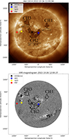 |
Fig. 1. Top: SDO AIA 193 Å image of the solar corona with the projected spacecraft positions. Bottom: SDO HMI magnetogram of the photosphere with the projected spacecraft positions (see legend). Black contours indicate CH boundaries. |
2.2. in situ measurements and CIR identification
The in situ measurements were performed by multiple instruments aboard five different spacecraft: 1) Solar Orbiter (SolO; Müller et al. 2020) with the Magnetometer (MAG; Horbury et al. 2020), the Solar Wind Analyzer suite (SWA; Owen et al. 2020). 2) Parker Solar Probe (PSP; Fox et al. 2016) with the instruments FIELDS (Bale et al. 2016), Solar Wind Electrons Alphas and Protons (SWEAP; Kasper et al. 2016), and Integrated Science Investigation of the Sun (IS⊙IS; McComas et al. 2016). 3) Solar Terrestrial Relations Observatory (STEREO-A; Kaiser 2005) with the instruments PLAsma and SupraThermal Ion Composition (PLASTIC; Galvin et al. 2008), in situ Measurements of PArticles and CME Transients (IMPACT; Luhmann et al. 2008) and Solar Wind Electron Analyzer (SWEA; Sauvaud et al. 2008). 4) Advanced Composition Explorer (ACE; Stone et al. 1998) with the Solar Wind Electron Proton Alpha Monitor (SWEPAM; McComas et al. 1998) and the Magnetic Field Experiment (MAG; Smith et al. 1998). Pitch angle distributions for L1 were provided by the Solar Wind Experiment (SWE; Ogilvie et al. 1995) aboard the Wind spacecraft. All data were downloaded from the Space Physics Data Facility (SPDF) repository1. After reduction, we used a time cadence of 0.5 h for each instrument.
In closest proximity to the Sun (0.32–0.41 AU), SolO provided magnetic field measurements by MAG and plasma parameters by its SWA suite. During the time period of interest, PSP was farther away from the Sun, being in its aphelion around 0.76 AU, between encounters #13 and #14, and providing plasma and magnetic field data with FIELDS, IS⊙IS and SWEAP. Longitudinally trailing behind Earth, at 1 AU orbit, STEREO-A and its PLASTIC and IMPACT instruments provided us with in situ measurements before the structures’ arrival at Earth. At the Lagrange point L1 close to Earth, we used magnetic field data from the MAG instrument aboard the ACE spacecraft and plasma parameters from its SWEPAM instrument. The spacecraft vary in their position, hence, their distances and longitudinal locations in the heliosphere change over time. This is summarized in Table 2 and visualized in Figure 2 covering the period 16 October 2022 – 2 November 2022.
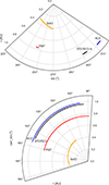 |
Fig. 2. Top: Spacecraft constellation in the HCI frame. Bottom: Spacecraft constellation in the Carrington corotating frame. The lines represent the positions of the spacecraft during the period of encountering the CIR/HSS. Date of first encounter for each spacecraft: SolO: October 18; PSP: October 21; STEREO-A: October 25; ACE: October 26. |
Spacecraft positions for the investigated time range.
Since the CIRs corotate with the Sun, they are best studied in situ in a corotating coordinate frame. Each time the CIRs cross a spacecraft, we monitor the time and the current Carrington longitude. Figure 2 shows the position of each spacecraft during their encounter with the CIRs and HSSs both in the Heliocentric Inertial (HCI) frame (top) and a corotating Carrington frame (bottom). In the inertial frame we can see, that only PSP and SolO are radially aligned. However, in the corotating frame, we can see that the satellite measurements at the selected dates probe the same Carrington longitudes and thus the same solar wind streams.
2.3. CIR four-region classification scheme
The different CIR regions are classified according to Belcher & Davis (1971), who identified four distinct regimes i) unperturbed slow, ii) perturbed slow, iii) perturbed fast, and iv) unperturbed fast solar wind. The perturbed slow and fast wind regions compose the CIR, which is followed by the unperturbed fast region. Figure 3 provides a sketch of the four regions of interest, which are investigated in this work, together with their plasma and magnetic field characteristics.
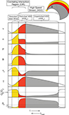 |
Fig. 3. Schematics of the structures and parameters defining the solar wind streams of interest. The uncolored (white) regions are plasma that is not of CH origin. The yellow regions mark the perturbed slow solar wind within the CIR, the red regions the perturbed part of the high speed stream (HSSp) within the CIR and the gray regions give the rarefaction region, i.e., the unperturbed part of the high speed stream (HSSu). From top to bottom: v: proton velocity, n: proton density; P: total pressure; B: total magnetic field strength; vT: tangential velocity; T: proton temperature; O7+/O6+: O7+/O6+ ratio; Sp: specific proton entropy. |
To identify the four CIR regions, we introduced a new technique which is based on various statistical results (Belcher & Davis 1971; Siscoe & Intriligator 1993; Crooker et al. 1999; Jian et al. 2006; Zhao et al. 2009; Xu & Borovsky 2015). Using plasma and magnetic field measurements, we identified the interfaces of the regions: forward pressure wave, stream interface (SI) between slow and fast solar wind, reverse pressure wave, and trailing edge. The forward pressure wave, i.e., the front boundary of the perturbed slow wind, is identified by the sudden increase in density, velocity, total magnetic field strength, pressure and proton temperature (see, e.g. Belcher & Davis 1971; Crooker et al. 1999). For total pressure we considered the sum of the magnetic and thermal pressure given as:
 (1)
(1)
where B is the magnetic field density, n is the proton density, and T is the proton temperature. Ideally, for total pressure, we would add alpha particle and electron pressure (see, e.g., Jian et al. 2006); however, these data are very scarce for the spacecraft we use during this period. The second boundary is the stream interface (SI), which usually coincides or is very close to the density peak. It is identified by finding the peak of the density and pressure profiles, as well as the inflection point (second derivative is zero) in the tangential velocity component (see, e.g. Belcher & Davis 1971; Gosling et al. 1978; Jian et al. 2006). The reverse pressure wave, which separates the perturbed fast wind from the unperturbed fast wind, is marked by a second steep drop in density after the initial decrease from the density peak (see Figure 3), the velocity maximum, as well as a drop in total magnetic field strength and pressure (see, e.g. Belcher & Davis 1971; Crooker et al. 1999). The trailing edge of the HSS is the location where CH plasma characteristics are no longer prevalent and can be identified by the O7+/O6+ ratio going above 0.145 (Zhao et al. 2009; Xu & Borovsky 2015). Where the O7+/O6+ is not available, we use the specific proton entropy Sp as a proxy with a threshold between 2.7 and 4 (see Siscoe & Intriligator 1993; Xu & Borovsky 2015). We define the specific proton entropy as:
 (2)
(2)
Also, the proton velocity arrives at a minimum at the end of the HSS. After careful testing, we decided to prefer these relative quantities to determine the stream boundaries. Using thresholds on absolute quantities, such as the absolute solar wind velocity or density, would make us more susceptible to the different instrument sensitivities and would not be reasonable to identify the evolving solar wind structures with distance from the Sun. All criteria and threshold values used to distinguish between the different CIR structures are summarized in Table 3. The error estimates stem from uncertainty in accurately identifying each interface. When multiple candidates were present for an interface, we selected the most prominent one manually and used the others to define the uncertainty range.
Classification scheme for CIR and HSS interfaces.
When the CH is close to a region on the Sun with the opposite polarity, CIRs are very often accompanied by the HCS. A density peak can form at the HCS location, which may become more prominent than the density peak at the SI, or in some cases, the two peaks may coincide. We therefore also checked for the prevalence of an HCS. The HCS is the boundary between different magnetic field polarities and has a steep decrease in magnetic field strength. It is also accompanied by a high plasma beta and density (Smith 2001; Liou & Wu 2021). Whenever solar wind electron in situ data were available, we checked the pitch angle of the suprathermal electrons, which changes direction in an HCS (criteria described in Smith 2001; Forsyth & Gosling 2001; Liou & Wu 2021).
2.4. Curvature
In this work, we investigated the large-scale structure of the regions mentioned in the previous section. When we identified the SI of a CIR/SIR, we recorded its position in terms of Carrington longitude, L, and distance to the Sun, R. Connecting the SI at two different spacecraft positions, we can calculate the angular displacement per radial unit between the two positions. Assuming the approximate shape of a Parker spiral, the angular displacement equals the average curvature of the spiral, C:
 (3)
(3)
leaving us with units of angle/length, which is commonly used to express the curvature of a curve.
2.5. Modeling
To gain a deeper understanding of the propagation and interaction of perturbed and unperturbed solar wind plasma and to identify potential shortcomings in our understanding, we compared the in situ profiles of CIRs and HSSs with three heliospheric models. These models cover different physical concepts and vary in complexity, starting from simple ballistic and kinematic solar wind models to sophisticated hydrodynamic and magneto-hydrodynamic ones:
-
Inelastic model
-
EUHFORIA (Pomoell & Poedts 2018).
The input conditions to the models are based on either the in situ measured velocity and density information from the spacecraft closest to the Sun or initiated by global photospheric magnetic field maps, which in our study were the GONG ADAPT (Global Oscillation Network Group–Air Force Data Assimilative Photospheric flux Transport – Arge et al. 2010; Hickmann et al. 2015). In the following, we shortly describe the different models.
2.5.1. Inelastic propagation
The first model we employed is a simple ballistic model with kinematic interaction between the plasma parcels. The algorithm propagates the in situ measured data points according to their velocities:
 (4)
(4)
 (5)
(5)
where Ri is the distance of the ith data point from the Sun measured by the spacecraft, λi is the Carrington longitude of the position of the data point, and Vi its radial velocity. Ω is the angular velocity of the solar rotation, which here has been set to 0.0096 rad/h and which corresponds to the average solar rotation rate. The time difference between two simulation time-steps Δt has been set to 0.5 h, which is equal to the cadence of the in situ data after reduction.
In the simulation, when two plasma parcels get within close distance of one another, they interact and propagate with a common velocity as derived by the equation for momentum conservation. The resulting velocity is calculated as:
 (6)
(6)
where Ni is the time-independent density of the ith data point.
2.5.2. HUXt
The second model is the Heliospheric Upwind Extrapolation (HUXt), a computationally efficient solar wind model based on a one-dimensional, incompressible, hydrodynamic fluid (Owens et al. 2020; Owens & Barnard 2024). HUXt can produce a time-dependent velocity profile for the entire heliosphere from an initial velocity field at an inner boundary. To run HUXt with in situ measurements requires preparing the data by ballistically back-mapping to a distance of 30 solar radii (similar to Section 2.5.1, but reverse). We performed this by ballistically backmapping the solar wind data measured by Solar Orbiter, which is the innermost spacecraft for our period of time.
2.5.3. EUHFORIA
The third model is EUHFORIA (Pomoell & Poedts 2018), which consists of a coronal and a heliospheric domain. The coronal domain is further divided into two modeling subdomains, the low and the upper corona. The low corona extends from the solar surface to the source surface, which for this study was set to 1.5 solar radii. We selected this value so that the modeled open field areas associated with the three CHs best agree with the observed areas in EUV. The magnetic field in the low corona is computed with the Potential Field Source Surface (PFSS) approximation (Altschuler & Newkirk 1969), using as input boundary conditions the GONG ADAPT global photospheric magnetic field map (Arge et al. 2010; Hickmann et al. 2015). The upper corona domain spans from just below the source surface up to 0.1 AU. The magnetic field topology there is computed using the Schatten Current Sheet (SCS, Schatten et al. 1969) model. The inner boundary of the SCS model is set a bit lower than the outer boundary of the PFSS model to account for unphysical kinks in the field lines described in McGregor et al. (2008). The numerical solver employed for both PFSS and SCS models is the spherical harmonics one, with l = 140 being the maximum degree used in the solid harmonic expansion. Based on the computed magnetic field topology, a global photospheric map of open and closed magnetic field regions is generated. Then, the distance from the open field area boundaries, which we denote with d, and the expansion factor for the associated magnetic flux tubes, which we denote with f, are calculated.
Since the PFSS and SCS models only extrapolate magnetic fields and do not provide plasma properties, EUHFORIA employs the following equation to set the plasma velocity at the upper boundary of the coronal regime:
![Mathematical equation: $$ v(f, d) = v_0 + \frac {v_1}{(1+f)^\alpha }\left [1{-}0.8\exp \left (-\left (\frac {d}{w}\right )^\beta \right )\right ]^3. $$](/articles/aa/full_html/2025/07/aa53096-24/aa53096-24-eq20.gif) (7)
(7)
Here, α = 0.22, β = 1.25, and w = 0.01 rad. Based on the calculated velocities the density is also derived. Further EUHFORIA model parameters for the upper boundary of the coronal model (0.1 AU) include the expected minimum and maximum speed (vmin = 275 km/s and vmax = 675 km/s respectively), the plasma pressure (P = 3.3 Pa), and the fast solar wind magnetic field (Bfast = 300 nT) and plasma density (nfast = 300 cm−3).
The heliospheric domain employs an ideal MHD model that extents from 0.1 to 2 AU. It uses as inner boundary the magnetic field and plasma conditions that are generated by the coronal domain models at 0.1 AU described above. In order to have the best match between model results and SolO in situ measurements, we rotated the result from the EUFHORIA heliospheric model by 30° in longitude. Such time shifts in the arrival of HSS peak speeds, of about one day and up to three days, are a well-documented issue (see, e.g., Owens et al. 2008; Reiss et al. 2016; Hinterreiter et al. 2019; Allen et al. 2020) for MHD models such as ENLIL (Odstrcil 2003) and EUHFORIA (presented here). Since the aim of this study is to compare the evolution of observed CIRs to that modeled while they propagate through the heliosphere, introducing a constant artificial time shift to correct for these timing errors in general in our study is justified.
3. Results
3.1. Structure of CIRs – Observations
Using the detection scheme described in Section 2.3 and Table 3, we identified the individual CIR and SIR regions from in situ measurements of the considered spacecraft. Figure 4 shows the velocity and density profiles and the identified regions for all spacecraft. Additionally, it serves as a chart showing the development of regions from one spacecraft to another. We refer to Figures A.1–A.4 in the Appendix for detailed plots of all other spacecraft’s in situ measured solar wind signatures, together with the applied parameters and thresholds for the extraction of the different CIR regions.
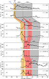 |
Fig. 4. Corotating interaction region and SIR regions identified in all spacecraft against the Carrington longitude. For each spacecraft we show the proton velocity and density. Blue: HCS; Yellow: perturbed slow find; Red: perturbed fast wind (HSSp); Gray: unperturbed fast wind (HSSu). |
The top two panels of Figure 4 show the velocity and density profiles measured by SolO, which provides the innermost in situ profiles at 0.32–0.41 AU. We identified an HCS (indicated with a solid blue line) within the perturbed slow solar wind (yellow). The perturbed slow solar wind indicates the start of the CIR. The perturbed fast wind, HSSp, is marked in red. The CIR has a longitudinal extension of 7.0±0.6 degrees. The CIR is followed by a rather long period of unperturbed fast wind, HSSu (marked in gray). The velocity profile of this long unperturbed fast wind seems to indicate two high-speed streams that have merged without a clear interaction region between them (cf. gray vertical line around Carrington longitude 156°). The solar wind temperature profile, shown in Figure A.1 in the Appendix, confirms this assumption and clearly shows two high-speed streams. The second HSS follows just behind the first one, without a visible trace of any interaction region in between. Both HSSs are similar in extent, with HSS1 spanning  degrees and HSS2 spanning
  degrees.
The in situ velocity and density signatures recorded by PSP, which was at an orbital distance of roughly 0.76 AU, are given in panels c and d of Figure 4. Here we see a wider CIR with an extent of 18.7±1.2 degrees and the HCS again in the perturbed slow wind. In contrast to the signatures from SolO closer to the Sun, HSS2 now started to interact with HSS1. Therefore, we identified a new SIR, which is the result of the two fast solar wind streams interacting, and marked it as perturbed fast wind in red. The SIR has an extent of  degrees. The extent of the unperturbed portion of HSS1, HSSu1, has decreased sharply from
  degrees to 10.5±0.6 degrees, which is roughly the width of the SIR. We propose that HSS2 ran into HSS1, piling up HSSu1 plasma and therefore reducing the extent of HSSu1.
In panels e and f of Figure 4, we present the in situ velocity and density profiles of STEREO-A, which is close to 1 AU (0.96 AU). We again identify the HCS within the perturbed slow wind region, with another density peak in front of it, consisting of piled up slow solar wind plasma. The velocity peak seems to have decreased in amplitude by the interaction with the slow wind. The SIR between HSS1 and HSS2 meanwhile has caught up to the CIR, producing a large, extended interaction region. The unperturbed part of HSS1 appears to have been compressed from both sides, by the slowed down CIR in front and the SIR, driven by the still fast HSS2 in the back. This produces another discontinuity within HSS1, between the CIR and the SIR, marked as a red vertical line. The extents of all structures barely change, but the unperturbed part HSS1 decreases sharply to zero, as it is being compressed.
Finally, the bottom two panels of Figure 4 show the in situ signatures measured by ACE at L1. Here, the density profile around the HCS has widened, and with it the extent of the perturbed slow solar wind, increasing the width of the CIR to  degrees. Especially in the density profile, it is apparent, that there are multiple discontinuities in the CIR and SIR regions, making it more difficult to attribute clearly defined regions to them. Due to the similarity in multiple plasma parameters to the signatures in STEREO-A, we can nonetheless identify the same regions. The SIR between HSS1 and HSS2 decreases to a width of
  degrees, and HSS2 decrease from
  in STEREO-A to
  . The results from the longitudinal extents of all structures are summarized in Table 4.
Longitudinal extent of regions.
Next, we analyzed the evolution of the structures, which is visualized in Figures 5 and 6. The measured longitudinal extent of each structure is plotted against the radial distance at which it was encountered. Figure 5 shows the evolution of the longitudinal extent of the structures with degrees as units, while 6 shows the same with kilometers as units. In gray, we show the unperturbed fast wind, HSSu, and in red the CIRs/SIRs (perturbed slow wind + HSSp). For reference, we also show the evolution of the longitudinal extent of a segment between two ideal Archimedean spirals that are separated by 13.9° and 30.9°, representing the longitudinal width of CH1 and CH2, respectively (see Figure 1 and Table 1). We speculate that CH1 and CH2 are related to HSS1 and HSS2 (see more detail in Section 3.2).
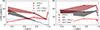 |
Fig. 5. Evolution of the extent of the structures. The black dots with the gray area represent the longitudinal extent of the unperturbed CH plasma (HSSu) and the red dots with the light red area are the longitudinal extent of the CIR/SIR (perturbed solar wind + HSSp). The dark red lines represent the longitudinal extent of the entire CIR/SIR + HSSu. The areas are the respective uncertainties. The purple line shows the extent of an area, that is bound by two Archimedean spirals, which are separated by 13.9° (CH1) and 30.9° (CH2). |
In the first panel of Figure 5, we see that the longitudinal extent of the CIR does not show a clear pattern; it changes significantly between each encounter at the various distances from the Sun. The extent of the following HSSu1 sharply decreases with distance and vanishes by its measurement at STEREO-A. The decrease in the extent of HSSu1 is due to its interaction with the slower plasma, preceding the CIR and from its tail being piled-up by the faster plasma following SIR.
The second panel of Figure 5 presents the same analysis for the SIR and HSSu2. The trend lines show a clear increase in extent for the SIR and a very stable HSSu2. the SIR encounters the high-speed, low-density plasma of HSSu1 on its front. Therefore, it slightly interacts with the HSSu1 plasma, piling up the HSSu1 plasma and thereby increasing its own extent while barely being slowed down. HSSu2, which follows the SIR, has almost the same velocity as the SIR and therefore can propagate freely, that is, almost without any interaction with the preceding plasma of the SIR. As there is no interaction for HSSu2, it follows very well the longitudinal extension of the Archimedean spiral related to CH2 with increasing distance to the Sun.
3.2. Model comparison and relation to CHs
In order to relate the HSS properties back to their source, i.e. CHs, we first identified the source regions with simple ballistic backmapping of the in situ measurements and also cross-checked with magnetic footpoints from PFSS extrapolation (results are provided in Figure A.5 in the Appendix). In the SolO profile, we see the velocity peak at roughly 175° Carrington longitude, with an amplitude of 750 km/s. Backmapping this feature traces it to a longitude of 186°, which, according to Table 1, falls right into the range of CH1. Similarly, tracing back the HSS measured by SolO, we find the footpoint to be at a Carrington longitude of roughly 150°, aligning with the center of CH2. Furthermore, we can confidently exclude any alternative sources further west for HSS1, as its polarity is positive, while the only other potential CH candidate has negative polarity and is located across the HCS. From the PFSS solution provided by SolarMACH (Gieseler et al. 2023) we find that they only partly agree with the backmapping results. From the PFSS footpoints both HSSs trace back to a region between CH1 and CH2. Hence, the PFSS maps suggest an alternative possibility that both HSS1 and HSS2 may originate from CH2. While this interpretation does not alter the evolution of the CIR/SIR structures under study, it may offer an alternative identification of the source region of the HSSs.
The in situ measurements analyzed in the previous section revealed interesting evolutionary characteristics of the various regions related to the CIR and the SIR. To cross-check whether similar results could be derived from simulations and for better understanding of the formation of these CIRs/SIRs, we have compared our observations to the three models described in Section 2.5. Figure 7 shows the results of the three different models in the corotating frame. The model results are shown in the background of each polar plot as a color gradient. The in situ measurements are plotted on top and accompanied by a single color line, indicating the spacecraft position.
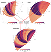 |
Fig. 7. Each plot shows the velocity profile of the associated model in the background color-coded and on top are the paths of the spacecraft with their respective in situ measured velocities. Next to the paths of the spacecraft, there are colored paths indicating the spacecraft (cf. Figure 2); yellow: SolO, red: PSP, black: STEREO-A and blue: ACE. In the online version of the article we also present a movie showing the inelastic propagation in process. |
The top-left panel of Figure 7 shows the result of the inelastic model, considering momentum conservation between the parcels of different velocity. Here we used as input data SolO in situ measurements, hence, we get a perfect match over the path of SolO. HSS1 and HSS2 are clearly visible as the two streams shown in purple in the modeled data. In the online version of this article, we show a movie of the inelastic model, where the slowing down and deflecting of HSS1 is visible.
As HSS1 encounters the slow stream ahead, it starts to inelastically collide, slowing down HSS1 and producing a stream interface and the CIR. This interaction increases the curvature, which results in a reasonable match with the in situ measurements from PSP, STEREO-A, and ACE, whose measurements are plotted on top of the modeled data. Looking at the in situ profile from PSP (red), the steep velocity gradient is at roughly 153 degrees, indicating the position of the SI of the CIR. This is missed by the model in the background by roughly 6°. The SI positions of STEREO-A and ACE are missed by 1° and 1.5°, respectively.
The top-right panel of Figure 7 shows the HUXt model results that were initiated by in situ measurements from SolO as input. Here we find a less steep curvature of HSS1 than in the inelastic model. The in situ signatures are therefore missed by a much larger margin. The position of the SI in the PSP data is missed by the model roughly by 15°, while the SIs measured by STEREO-A and ACE are missed by 9° and 14°, respectively.
The bottom panel of Figure 7 shows the model result from EUHFORIA. Both HSSs are modeled well and match SolO measurements, but, again, the curvature is not steep enough to match the observed velocity profiles at the outer spacecraft correctly. The profile for SolO fits well, despite not having in situ input to the model. For PSP, the model is almost as far off as HUXt, by 14°. Further out, EUHFORIA fits slightly better, missing the SI of STEREO-A by 6° and the one of ACE by 9°.
Concluding, we don’t find an increasing deviation between the modeled and observed HSS1 and the CIR locations with increasing distance from the Sun. Rather, we find that the profile, measured by PSP at roughly 0.76 AU is the most difficult to predict. To correctly connect the CIR measured at SolO and PSP, the spiral has to have a very steep slope of 73±0.1 deg/AU, and to connect PSP with STEREO-A and ACE, the spiral has to have a slope of just 24±20 deg/AU. The average spiral slope is 57±9 deg/AU. This is not being reproduced by any model. The models’ spiral curvature of the SI at the CIR range from 33.7±1 deg/AU for the HUXt run to 56±1 deg/AU for the inelastic run. None predict the sharp change of curvature around PSP. A summary of the curvatures for the CIR measured and derived from models are given in Table 5.
Stream interface curvature.
Next, we investigated in more detail the accuracy of the modeled velocity profiles. In Figures 8 and 9, we present for each spacecraft the observed and modeled velocity profiles. The black and gray vertical lines indicate the position of the stream interface to the preceding slow solar wind as identified in the in situ data as described in Section 2.2 and as identified in the modeled data as the maximum in the velocity gradient. The red vertical line indicates for reference the position of the SI of the CIR between the slow solar wind and HSS1. We did not apply the solar wind classification scheme from Section 2.3 here, since the models do not provide all required parameters. Therefore, we also do not go into detail about the modeled longitudinal extent of any regions, but focus solely on the curvature of the first SI.
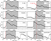 |
Fig. 8. in situ velocity profile (top panel) and each model velocity profile for Solar Orbiter and PSP. The vertical lines indicate the position of the stream interface; black: the position of the SI for each model; red: the position of the SI in the in situ data for comparison. |
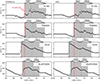 |
Fig. 9. in situ velocity profile (top panel) and each model velocity profile for STEREO-A and ACE. The vertical lines indicate the position of the SI; black: the position of the SI for each model; red: the position of the SI in the in situ data for comparison. |
In Figure 8, we compared the modeled velocity profiles with the observed ones for SolO and PSP. At SolO’s location, all the model runs predict well the stream interface to the preceding slow solar wind. For the in situ models, this is since we drive the models by SolO’s in situ observations; for EUHFORIA, this is since we have introduced in Section 2.5.3 an artificial longitudinal shift so that the modeled velocity profile at SolO best match the observed one. At PSP’s location further out, there are large differences between the positions of the modeled stream interfaces and the observed ones. HUXt and EUHFORIA are off by roughly 15° and the inelastic model is off by less than 6°. Interestingly, in contrast to the modeled stream interfaces to the preceding slow solar wind, the modeled positions of HSS2 are quite accurate for the models that are driven by the in situ data.
In Figure 9 we present the modeled velocity profiles for STEREO-A and ACE, which are located at around 1 AU. Here, the positions of the SI fit better, but they are still all off to the left side by 5–10° for both spacecraft, except for the inelastic model, which is only off by 1° and 1.5°, each. For both spacecraft we see large discrepancies in the modeled velocity profiles of the CIR and HSS1 to the observations. Again, the modeled velocity profiles for HSS2 fit better.
In conclusion, none of the models can reproduce well the shape of the CIR and HSS1, but they do roughly reproduce the shape of the SIR and HSS2. This shows that all the models cannot simulate well the interaction regions to the preceding slow solar wind; but all models work reasonable well to simulate the propagation of HSS plasma outside CIRs.
4. Discussion
4.1. CIR and SIR formation and radial evolution
Investigating the in situ signature measured by SolO, we find that the CIR has already formed at roughly 0.32 AU, while the SIR has not yet formed at 0.35 AU. These results agree well with the work from Allen et al. (2020), who concluded that CIRs most likely are either fully formed, or, are in the formation process between 0.3 and 0.4 AU.
For the CIR evolution in interplanetary space, studies reveal divergent perspectives, indicating either increasing widths or variations over distance. Schwartz & Marsch (1983) and Rivera et al. (2024) investigated a single patch of solar wind related to HSSs that passed two spacecraft, both of which give evidence for a compression of the embedded solar wind plasma by roughly 10% between 0.5 and 0.7 AU (Schwartz & Marsch 1983) but also between 0.06 AU and 0.6 AU (Rivera et al. 2024). Garton et al. (2018) show in a statistical study that the longitudinal extent of HSSs would increase over distance by relating the HSS width measured at 1 AU to the longitudinal extent of the CH. From this, they found that the HSS extent at 1 AU is about 1.2 times greater than the extent of the associated CH. Beyond 1 AU, Geyer et al. (2021) conclude that the CIR longitudinal extent as measured at Earth is similar to the one at Mars and that major changes in the stream evolution occur close to SI.
CH1 has a longitudinal extent of 13.9° and HSS1 a longitudinal extent of 11.8° at ACE and CH2 has a longitudinal extent of 30.9° and HSS2 a longitudinal extent of 35.0° at ACE. Both values agree fairly well with speculations of their link to CH1 and CH2 (see also statistical results by Garton et al. 2018). In that respect, HSS1 appears to be compressed with distance, as the slow solar wind ahead and the fast solar wind from behind push from either side while HSS2 stays roughly at the expected extent from the width of CH2 (cf. Figure 5).
However, an interpretation of the evolution of the CIR extent appears more difficult. For the CIR, we find that its extent increases from the locations at SolO to PSP, but then appear smaller again towards STEREO-A. At ACE, there is again a drastic increase of its extent. Therefore, we speculate that the extent of the CIR seems first to increase as reported by Garton et al. (2018) and then gets compressed again at 0.76 AU and 1 AU, i.e., between PSP and the spacecraft STEREO-A, similar to Schwartz & Marsch (1983) and Rivera et al. (2024). Over time, between the measurements of STEREO-A and ACE, the CIR accumulates more plasma, increasing its width.
Schwenn & Marsch (1990) describe the evolution of the radial and longitudinal widths of CIRs as a balance between plasma pressure effects and kinetic steepening. Close to the Sun, the characteristic speed at which pressure signals propagate is high, preventing significant compression and density enhancements within CIRs. Due to the low pressure in the CIR, lateral flow deflections at the stream interface (SI) remain minimal, keeping the CIR narrow. This aligns with our observation of a narrow CIR at 0.32 AU. Beyond 0.4 AU and up to approximately 1 AU, the characteristic wave speed decreases, leading to stronger compression within the CIR. Consequently, stream deflections at the SI intensify, causing the CIR to widen. This trend is evident in PSP measurements at 0.76 AU, where the CIR appears significantly broader (cf. 5). However, kinematic steepening counteracts this widening effect. We believe that this interplay between pressure-driven expansion and kinematic steepening largely explains the variations observed in CIRs at different distances from the Sun.
In contrast to the CIR, the SIR we observe evolves over distance with a constant angular width with a slight decrease at the end (see Figures 5 and 6). From this, we can conclude that HSS2 experiences only a weak interaction with HSS1.
4.2. Curvature
Here we want to highlight one specific result of our analysis due to its peculiarity. There is a strong change in the curvature when comparing the appearance in time and location of the SI of the CIR. The connecting spiral between the SI positions in SolO and PSP measurements has a curvature of 73±0.1 deg/AU. This is twice as large as the nominal Parker spiral, which is about 35 deg/AU for an average speed of the HSS of ca. 650 km/s. On the contrary, we derive a very gentle curvature when connecting the SI of the CIR between PSP and the STEREO-A and ACE spacecraft at 1 AU (24±20 deg/AU). None of the models is predicting such a strong change in the curvature, and none can reproduce the steep inner curvature. The ‘inelastic’ model comes closest with 56±2 deg/AU (Table 5).
The curvature of HSS2, however, is close to the nominal Parker spiral (35.2 deg/AU), which we would expect from a freely propagating HSS without acceleration. We do not rule out a slight acceleration and resulting interaction with the plasma ahead. Recent studies have shown that the solar wind plasma can get accelerated even up to Venus distance (Rivera et al. 2024).
4.3. Discussion on discrepancies
For the peculiarities in the radial evolution of the longitudinal extent as well as the curvature of the positions of the SI as observed in CIR1, we speculate about possible explanations and shortcomings.
The models used in this study assume a steady-state corona and solar wind structure in the heliosphere. However, the corona is dynamically changing. Especially, changes in the magnetic field surrounding the CH might have a strong influence on the evolution and interaction of the slow and fast streams over time and distance. Therefore, a shift of the modeling approach to time-dependent coronal input and a corresponding time-dependent solar wind outflow should be considered. First attempts of time-dependent modeling show more realistic CIR profiles, as these account for the dynamic reconstruction of the solar wind in the heliosphere (e.g., Linker et al. 2016; Merkin et al. 2016; Owens et al. 2024).
A source of observational uncertainty is that the spacecraft are not temporally aligned (see Table 2). Due to their different longitudinal position in the inertial frame, the spacecraft probe the CIR up to 9 days apart. Within those days, the CIR observed at the different spacecraft might have evolved due to changes in the solar magnetic field, complicating the interpretation of the observational results.
Due to the three-dimensional geometry of the CIR, the spacecraft are not perfectly latitudinally aligned and might probe different regions within the CIR. This is shown in Table 2. The latitudinal differences are within three degrees, so they are not very large. However, in the case that the spacecraft measures the latitudinal CIR flank, even such small differences can result in quite different measured velocity profiles and thus contribute largely to uncertainties (e.g., see Gómez-Herrero et al. 2011; Hofmeister et al. 2020).
An HCS is located within the observed CIR, as described in Section 3.1. The presence of the HCS might be related to the strong change in curvature due to a possible deflection of the HSS on the HCS. Similar behavior has been found for CMEs (see, e.g., Gopalswamy et al. 2009; Wang et al. 2023). This deflection is generally not just in the ecliptic plane. The HSS could be deflected to higher latitudes, resulting in a change in its measurement profile – showing a direct impact at one spacecraft location, while only a glancing hit at another (see Hofmeister et al. 2018). We expect the HCS to only have a small effect on the CIR, but it might be a compounding factor to the effect. Hence, our study shows that we still do not understand the three-dimensional behavior of CIRs in the heliosphere.
In the models, the physical equations that describe the interaction between various solar wind streams might be inaccurate. This is shown in our study, as the curvature in the inner region (0.32–0.76 AU) is far steeper than any model predicts. Even the most aggressive interaction model, the inelastic model, underestimates the curvature by 24% (56±2 deg/AU compared to 73±0.1 deg/AU). For this strong underestimation, we see several reasons. For the inelastic model, interaction is only considered in the radial direction. However, the interaction process between the HSS and the preceding slow solar wind acts in all three dimensions, not just the radial one. For HUXt, the model misses the necessary MHD processes to accurately describe the CIR evolution. And for EUHFORIA, the model does not include kinetic processes, which probably play a role. Interestingly, the simplest model assuming only inelastic collisions produces the curvature with the best agreement to the observations.
5. Conclusion
In this work, we have analyzed the two-dimensional structure of two HSSs and their CIRs and SIRs by exploiting a favorable multi-spacecraft constellation consisting of SolO, PSP, STEREO-A, and ACE, which were at different distances from the Sun. We introduced a scheme to identify different regions of the observed CIRs in the in situ data and compared these to the modeling results of an inelastic solar wind model, HUXt, and EUFHORIA. We found the following
-
The CIR is already fully formed at 0.32 AU.
-
An SIR between HSS1 and HSS2 forms between 0.35 AU and 0.76 AU.
-
The longitudinal extents of the CIR and the associated HSS1 change significantly, while the SIR and the associated HSS2 roughly follow an ideal spiral structure.
-
The longitudinal extent of the entire first stream, CIR + HSSu1, does not exhibit a predictable trend over distance. Instead, it shows a complex pattern of varying widths at the various distances from the Sun.
-
In addition, the CIR shows an extremely steep spiral with a curvature of 73±0.1 deg/AU between 0.32 AU and 0.76 AU.
None of the models we used can explain the observed behavior of the CIRs/SIRs and HSSs in this study. The reasons might be the temporal evolution of the corona and the associated solar wind structures, an inaccurate modeling of the three-dimensional shape of the solar wind structures, or propagational effects such as deflections at the HCS. Future in situ measurements of multi-spacecraft constellations, particularly involving SolO going out of ecliptic in 2025, might shed more light on these issues.
Data availability
Movie associated to Fig. 7 is available at https://www.aanda.org
Acknowledgments
D.M. and M.T. acknowledge the support by the FFG/ASAP Program under grant CASPER (900588). S.J.H. acknowledges support from the NSF AST Grant AST-2005887. E.A. acknowledges support from the Finnish Research Council, formerly Academy of Finland (Research Fellow grant number 355659). S.G.H. acknowledges funding by the Austrian Science Fund (FWF): Erwin-Schrödinger fellowship J-4560.
References
- Allen, R. C., Lario, D., Odstrcil, D., et al. 2020, ApJS, 246, 36 [Google Scholar]
- Allen, R. C., Ho, G. C., Mason, G. M., et al. 2021, Geophys. Res. Lett., 48, e91376 [NASA ADS] [CrossRef] [Google Scholar]
- Al-Shakarchi, D. A., & Morgan, H. 2020, Ap&SS, 365, 61 [Google Scholar]
- Altschuler, M. D., & Newkirk, G. 1969, Sol. Phys., 9, 131 [NASA ADS] [CrossRef] [Google Scholar]
- Arge, C. N., Henney, C. J., Koller, J., et al. 2010, in Twelfth International Solar Wind Conference, eds. M. Maksimovic, K. Issautier, N. Meyer-Vernet, M. Moncuquet, & F. Pantellini, (AIP), AIP Conf. Ser., 1216, 343 [NASA ADS] [Google Scholar]
- Bale, S. D., Goetz, K., Harvey, P. R., et al. 2016, Space Sci. Rev., 204, 49 [Google Scholar]
- Bale, S. D., Drake, J. F., McManus, M. D., et al. 2023, Nature, 618, 252 [NASA ADS] [CrossRef] [Google Scholar]
- Belcher, J. W., & Davis, L. Jr. 1971, J. Geophys. Res., 76, 3534 [NASA ADS] [CrossRef] [Google Scholar]
- Bohlin, J. D. 1977, Sol. Phys., 51, 377 [NASA ADS] [CrossRef] [Google Scholar]
- Cranmer, S. R., Gibson, S. E., & Riley, P. 2017, Space Sci. Rev., 212, 1345 [Google Scholar]
- Crooker, N. U., Gosling, J. T., Bothmer, V., et al. 1999, Space Sci. Rev., 89, 179 [Google Scholar]
- Forsyth, R. J., & Gosling, J. T. 2001, in The Heliosphere Near Solar Minimum. The Ulysses Perspective, eds. A. Balogh, R. G. Marsden, & E. J. Smith, 107 [Google Scholar]
- Fox, N. J., Velli, M. C., Bale, S. D., et al. 2016, Space Sci. Rev., 204, 7 [Google Scholar]
- Galvin, A. B., Kistler, L. M., Popecki, M. A., et al. 2008, Space Sci. Rev., 136, 437 [Google Scholar]
- Garton, T. M., Murray, S. A., & Gallagher, P. T. 2018, ApJ, 869, L12 [NASA ADS] [CrossRef] [Google Scholar]
- Geyer, P., Temmer, M., Guo, J., & Heinemann, S. G. 2021, A&A, 649, A80 [NASA ADS] [CrossRef] [EDP Sciences] [Google Scholar]
- Geyer, P., Dumbović, M., Temmer, M., et al. 2023, A&A, 672, A168 [NASA ADS] [CrossRef] [EDP Sciences] [Google Scholar]
- Gieseler, J., Dresing, N., Palmroos, C., et al. 2023, Front. Astron. Space Sci., 9, 1058810 [CrossRef] [Google Scholar]
- Gómez-Herrero, R., Malandraki, O., Dresing, N., et al. 2011, J. Atmos. Sol. Terr. Phys., 73, 551 [CrossRef] [Google Scholar]
- Gopalswamy, N., Mäkelä, P., Xie, H., Akiyama, S., & Yashiro, S. 2009, J. Geophys. Res.: Space Phys., 114, A00A22 [Google Scholar]
- Gosling, J. T., Asbridge, J. R., Bame, S. J., & Feldman, W. C. 1978, J. Geophys. Res., 83, 1401 [NASA ADS] [CrossRef] [Google Scholar]
- Heinemann, S. G., Temmer, M., Heinemann, N., et al. 2019a, Sol. Phys., 294, 144 [NASA ADS] [CrossRef] [Google Scholar]
- Heinemann, S. G., Temmer, M., Farrugia, C. J., et al. 2019b, Sol. Phys., 294, 121 [NASA ADS] [CrossRef] [Google Scholar]
- Heinemann, S. G., Jerčić, V., Temmer, M., et al. 2020, A&A, 638, A68 [EDP Sciences] [Google Scholar]
- Heinemann, S. G., Sishtla, C., Good, S., Grandin, M., & Pomoell, J. 2024, ApJ, 963, L25 [Google Scholar]
- Hickmann, K. S., Godinez, H. C., Henney, C. J., & Arge, C. N. 2015, Sol. Phys., 290, 1105 [NASA ADS] [CrossRef] [Google Scholar]
- Hinterreiter, J., Magdalenic, J., Temmer, M., et al. 2019, Sol. Phys., 294, 170 [NASA ADS] [CrossRef] [Google Scholar]
- Hofmeister, S. J., Veronig, A., Temmer, M., et al. 2018, J. Geophys. Res.: Space Phys., 123, 1738 [Google Scholar]
- Hofmeister, S. J., Veronig, A. M., Poedts, S., Samara, E., & Magdalenic, J. 2020, ApJ, 897, L17 [NASA ADS] [CrossRef] [Google Scholar]
- Hofmeister, S. J., Asvestari, E., Guo, J., et al. 2022, A&A, 659, A190 [NASA ADS] [CrossRef] [EDP Sciences] [Google Scholar]
- Horbury, T. S., O’Brien, H., Carrasco Blazquez, I., et al. 2020, A&A, 642, A9 [NASA ADS] [CrossRef] [EDP Sciences] [Google Scholar]
- Hou, C., Rouillard, A. P., He, J., et al. 2024, ApJ, 968, L28 [NASA ADS] [CrossRef] [Google Scholar]
- Jian, L., Russell, C. T., Luhmann, J. G., & Skoug, R. M. 2006, Sol. Phys., 239, 337 [NASA ADS] [CrossRef] [Google Scholar]
- Jian, L. K., Russell, C. T., Luhmann, J. G., Galvin, A. B., & MacNeice, P. J. 2009, Sol. Phys., 259, 345 [NASA ADS] [CrossRef] [Google Scholar]
- Jian, L. K., Russell, C. T., Luhmann, J. G., et al. 2011, Sol. Phys., 273, 179 [NASA ADS] [CrossRef] [Google Scholar]
- Kaiser, M. L. 2005, Adv. Space Res., 36, 1483 [NASA ADS] [CrossRef] [Google Scholar]
- Karna, N., Berger, M. A., Asgari-Targhi, M., Paulson, K., & Fujiki, K. 2022, ApJ, 925, 62 [Google Scholar]
- Kasper, J. C., Abiad, R., Austin, G., et al. 2016, Space Sci. Rev., 204, 131 [Google Scholar]
- Kay, C., Nieves-Chinchilla, T., Hofmeister, S. J., & Palmerio, E. 2022, Space Weather, 20, e2022SW003165 [NASA ADS] [Google Scholar]
- Koukras, A., Dolla, L., & Keppens, R. 2025, A&A, 694, A134 [NASA ADS] [CrossRef] [EDP Sciences] [Google Scholar]
- Krieger, A. S., Timothy, A. F., & Roelof, E. C. 1973, Sol. Phys., 29, 505 [NASA ADS] [CrossRef] [Google Scholar]
- Lemen, J. R., Title, A. M., Akin, D. J., et al. 2012, Sol. Phys., 275, 17 [Google Scholar]
- Linker, J. A., Caplan, R. M., Downs, C., et al. 2016, J. Phys. Conf. Ser., 719, 012012 [NASA ADS] [CrossRef] [Google Scholar]
- Liou, K., & Wu, C. -C. 2021, ApJ, 920, 39 [NASA ADS] [CrossRef] [Google Scholar]
- Liu, Y., Shen, F., & Yang, Y. 2019, ApJ, 887, 150 [NASA ADS] [CrossRef] [Google Scholar]
- Lowder, C., Qiu, J., & Leamon, R. 2017, Sol. Phys., 292, 18 [NASA ADS] [CrossRef] [Google Scholar]
- Luhmann, J. G., Curtis, D. W., Schroeder, P., et al. 2008, Space Sci. Rev., 136, 117 [Google Scholar]
- McComas, D. J., Bame, S. J., Barker, P., et al. 1998, Space Sci. Rev., 86, 563 [CrossRef] [Google Scholar]
- McComas, D. J., Elliott, H. A., Schwadron, N. A., et al. 2003, Geophys. Res. Lett., 30, 1517 [Google Scholar]
- McComas, D. J., Elliott, H. A., Gosling, J. T., & Skoug, R. M. 2006, Geophys. Res. Lett., 33, L09102 [NASA ADS] [Google Scholar]
- McComas, D. J., Alexander, N., Angold, N., et al. 2016, Space Sci. Rev., 204, 187 [Google Scholar]
- McGregor, S. L., Hughes, W. J., Arge, C. N., & Owens, M. J. 2008, J. Geophys. Res.: Space Phys., 113, A08112 [Google Scholar]
- Merkin, V. G., Lyon, J. G., Lario, D., Arge, C. N., & Henney, C. J. 2016, J. Geophys. Res.: Space Phys., 121, 2866 [NASA ADS] [CrossRef] [Google Scholar]
- Milošić, D., Temmer, M., Heinemann, S. G., et al. 2023, Sol. Phys., 298, 45 [Google Scholar]
- Müller, D., St. Cyr, O. C., Zouganelis, I., et al. 2020, A&A, 642, A1 [Google Scholar]
- Nolte, J. T., Krieger, A. S., Timothy, A. F., et al. 1976, Sol. Phys., 46, 303 [NASA ADS] [CrossRef] [Google Scholar]
- Odstrcil, D. 2003, Adv. Space Res., 32, 497 [CrossRef] [Google Scholar]
- Ogilvie, K., Chornay, D., Fritzenreiter, R., et al. 1995, Space Sci. Rev., 71, 55 [Google Scholar]
- Owen, C. J., Bruno, R., Livi, S., et al. 2020, A&A, 642, A16 [EDP Sciences] [Google Scholar]
- Owens, M., & Barnard, L. 2024, https://doi.org/10.5281/zenodo.10842659 [Google Scholar]
- Owens, M. J., Spence, H. E., McGregor, S., et al. 2008, Space Weather, 6, S08001 [Google Scholar]
- Owens, M., Lang, M., Barnard, L., et al. 2020, Sol. Phys., 295, 43 [NASA ADS] [CrossRef] [Google Scholar]
- Owens, M., Barnard, L., Arge, C., et al. 2024, Solar-wind Modelling: The Importance of Boundary Evolution, https://doi.org/10.21203/rs.3.rs-4876476/v1, pREPRINT (Version 1) [Google Scholar]
- Parker, E. N. 1958, ApJ, 128, 664 [Google Scholar]
- Perrone, D., Stansby, D., Horbury, T. S., & Matteini, L. 2019, MNRAS, 483, 3730 [Google Scholar]
- Pesnell, W. D., Pesnell, W. D., Thompson, B. J., & Chamberlin, P. C. 2012, Sol. Phys., 275, 3 [NASA ADS] [CrossRef] [Google Scholar]
- Pomoell, J., & Poedts, S. 2018, J. Space Weather Space Clim., 8, A35 [NASA ADS] [CrossRef] [EDP Sciences] [Google Scholar]
- Reiss, M. A., Temmer, M., Veronig, A. M., et al. 2016, Space Weather, 14, 495 [NASA ADS] [CrossRef] [Google Scholar]
- Richardson, I. G. 2018, Living Rev. Sol. Phys., 15, 1 [Google Scholar]
- Richter, A. K., & Luttrell, A. H. 1986, J. Geophys. Res., 91, 5873 [NASA ADS] [CrossRef] [Google Scholar]
- Riley, P., Linker, J. A., & Mikić, Z. 2002, J. Geophys. Res.: Space Phys., 107, 1136 [Google Scholar]
- Rivera, Y. J., Badman, S. T., Stevens, M. L., et al. 2024, Science, 385, 962 [NASA ADS] [CrossRef] [Google Scholar]
- Rotter, T., Veronig, A. M., Temmer, M., & Vršnak, B. 2012, Sol. Phys., 281, 793 [CrossRef] [Google Scholar]
- Sauvaud, J. A., Larson, D., Aoustin, C., et al. 2008, in The STEREO Mission (New York, NY: Springer), 227 [Google Scholar]
- Schatten, K. H., Wilcox, J. M., & Ness, N. F. 1969, Sol. Phys., 6, 442 [Google Scholar]
- Scherrer, P. H., Schou, J., Bush, R. I., et al. 2012, Sol. Phys., 275, 207 [Google Scholar]
- Schwartz, S. J., & Marsch, E. 1983, J. Geophys. Res., 88, 9919 [NASA ADS] [CrossRef] [Google Scholar]
- Schwenn, R., & Marsch, E. 1990, Physics of the Inner Heliosphere I. Large-Scale Phenomena (New York, Berlin, Heidelberg: Springer-Verlag) [Google Scholar]
- Sheeley, N. R. J., Harvey, J. W., & Feldman, W. C., 1976, Sol. Phys., 49, 271 [Google Scholar]
- Simunac, K., Kistler, L., Galvin, A., et al. 2009, Sol. Phys., 259, 323 [Google Scholar]
- Siscoe, G., & Intriligator, D. 1993, Geophys. Res. Lett., 20, 2267 [Google Scholar]
- Smith, E. J. 2001, J. Geophys. Res., 106, 15819 [NASA ADS] [CrossRef] [Google Scholar]
- Smith, E. J., & Wolfe, J. H. 1976, Geophys. Res. Lett., 3, 137 [Google Scholar]
- Smith, C. W., L’Heureux, J., Ness, N. F., et al. 1998, Space Sci. Rev., 86, 613 [Google Scholar]
- Stone, E. C., Frandsen, A. M., Mewaldt, R. A., et al. 1998, Space Sci. Rev., 86, 1 [Google Scholar]
- Tsurutani, B. T., Gonzalez, W. D., Gonzalez, A. L. C., et al. 2006, J. Geophys. Res.: Space Phys., 111, A07S01 [NASA ADS] [Google Scholar]
- Viall, N. M., & Borovsky, J. E. 2020, J. Geophys. Res.: Space Phys., 125, e26005 [NASA ADS] [CrossRef] [Google Scholar]
- Vršnak, B., Temmer, M., & Veronig, A. M. 2007, Sol. Phys., 240, 315 [Google Scholar]
- Wang, J., Liu, S., & Luo, B. 2023, Adv. Space Res., 72, 5263 [Google Scholar]
- Xu, F., & Borovsky, J. E. 2015, J. Geophys. Res.: Space Phys., 120, 70 [NASA ADS] [CrossRef] [Google Scholar]
- Zhao, L., Zurbuchen, T. H., & Fisk, L. A. 2009, Geophys. Res. Lett., 36, L14104 [NASA ADS] [CrossRef] [Google Scholar]
Appendix A: in situ measurements and connectivity to the source regions
Figures A.1 to A.4 show for all spacecraft under investigation the magnetic field and plasma parameters measured at their specific location. In addition, the parameters and thresholds used for the extraction of the different CIR regions and HCS are indicated in each plot. Figure A.5 gives results for deriving the source regions from HSS1 and HSS2 using ballistic backmapping and the magnetic connectivity tool from SolarMACH based on PFSS (Gieseler et al. 2023). For the ballistic backmapping there is no latitude information. Deriving the connectivity from PFSS usually is prone to uncertainties in the range of 10° due to the choice of surface heights (see, e.g., Koukras et al. 2025). Backmapping HSS1 and HSS2 from in situ measurements of all the spacecraft in this study, we derive a statistical distribution of solar wind sources for HSS1 and HSS2 as well as for the solar wind measured before and after.
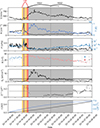 |
Fig. A.1. Solar Orbiter in situ signature. The blue line represents the HCS, the yellow area is the perturbed slow wind and the gray area is the unperturbed fast wind. From top to bottom: V:proton velocity, N:proton density; T:proton temperature; P:total pressure; β: plasma beta; B:total magnetic field strength; Sp:specific proton entropy; O7+/O6+: O7+/O6+ ratio; r: distance of the spacecraft to the Sun; LAT: latitude of the spacecraft in HCI. Error bars on top of the plot show the uncertainties in the region classification. |
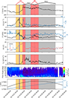 |
Fig. A.2. Parker Solar Probe in situ signature. The blue line represents the HCS, the yellow area is the perturbed slow wind, the red area is the perturbed fast wind and the gray area is the unperturbed fast wind. From top to bottom: V:proton velocity, N:proton density; T:proton temperature; P:total pressure; β: plasma beta; B:total magnetic field strength; Sp:specific proton entropy; suprathermal pitch angle distribution; r: distance of the spacecraft to the Sun; LAT: latitude of the spacecraft in HCI. Error bars on top of the plot show the uncertainties in the region classification. |
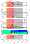 |
Fig. A.3. STEREO in situ signature. The blue line represents the HCS, the yellow area is the perturbed slow wind, the red area is the perturbed fast wind and the gray area is the unperturbed fast wind. From top to bottom: V:proton velocity, N:proton density; T:proton temperature; P:total pressure; β: plasma beta; B:total magnetic field strength; Sp:specific proton entropy; suprathermal pitch angle distribution; r: distance of the spacecraft to the Sun; LAT: latitude of the spacecraft in HCI. Error bars on top of the plot show the uncertainties in the region classification. |
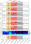 |
Fig. A.4. ACE in situ signature. The blue line represents the HCS, the yellow area is the perturbed slow wind, the red area is the perturbed fast wind and the gray area is the unperturbed fast wind. From top to bottom: V:proton velocity, N:proton density; T:proton temperature; P:total pressure; β: plasma beta; B:total magnetic field strength; VT: tangential proton velocity; Sp:specific proton entropy; suprathermal pitch angle distribution provided by Wind spacecraft; r: distance of the spacecraft to the Sun; LAT: latitude of the spacecraft in HCI. Error bars on top of the plot show the uncertainties in the region classification. |
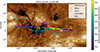 |
Fig. A.5. Backmapping of in situ data to their source surface. The empty circles show magnetic footpoints from PFSS extrapolation, color-coded with the identified solar wind region found in situ. The colored discs show the ballistic backmapping of Solar Orbiter in situ data during its encounter with the SIRs and HSSs, color-coded with the measured solar wind velocity. The velocity enhancements in the ballistically backmapped data correspond with HSS1 and HSS2. The black dotted line shows the position of the HCS, according to the PFSS solution. |
All Tables
All Figures
|
Fig. 1. Top: SDO AIA 193 Å image of the solar corona with the projected spacecraft positions. Bottom: SDO HMI magnetogram of the photosphere with the projected spacecraft positions (see legend). Black contours indicate CH boundaries. |
| In the text | |
|
Fig. 2. Top: Spacecraft constellation in the HCI frame. Bottom: Spacecraft constellation in the Carrington corotating frame. The lines represent the positions of the spacecraft during the period of encountering the CIR/HSS. Date of first encounter for each spacecraft: SolO: October 18; PSP: October 21; STEREO-A: October 25; ACE: October 26. |
| In the text | |
|
Fig. 3. Schematics of the structures and parameters defining the solar wind streams of interest. The uncolored (white) regions are plasma that is not of CH origin. The yellow regions mark the perturbed slow solar wind within the CIR, the red regions the perturbed part of the high speed stream (HSSp) within the CIR and the gray regions give the rarefaction region, i.e., the unperturbed part of the high speed stream (HSSu). From top to bottom: v: proton velocity, n: proton density; P: total pressure; B: total magnetic field strength; vT: tangential velocity; T: proton temperature; O7+/O6+: O7+/O6+ ratio; Sp: specific proton entropy. |
| In the text | |
|
Fig. 4. Corotating interaction region and SIR regions identified in all spacecraft against the Carrington longitude. For each spacecraft we show the proton velocity and density. Blue: HCS; Yellow: perturbed slow find; Red: perturbed fast wind (HSSp); Gray: unperturbed fast wind (HSSu). |
| In the text | |
|
Fig. 5. Evolution of the extent of the structures. The black dots with the gray area represent the longitudinal extent of the unperturbed CH plasma (HSSu) and the red dots with the light red area are the longitudinal extent of the CIR/SIR (perturbed solar wind + HSSp). The dark red lines represent the longitudinal extent of the entire CIR/SIR + HSSu. The areas are the respective uncertainties. The purple line shows the extent of an area, that is bound by two Archimedean spirals, which are separated by 13.9° (CH1) and 30.9° (CH2). |
| In the text | |
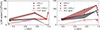 |
Fig. 6. Same as Figure 5, but longitudinal extents are given in kilometers. |
| In the text | |
|
Fig. 7. Each plot shows the velocity profile of the associated model in the background color-coded and on top are the paths of the spacecraft with their respective in situ measured velocities. Next to the paths of the spacecraft, there are colored paths indicating the spacecraft (cf. Figure 2); yellow: SolO, red: PSP, black: STEREO-A and blue: ACE. In the online version of the article we also present a movie showing the inelastic propagation in process. |
| In the text | |
|
Fig. 8. in situ velocity profile (top panel) and each model velocity profile for Solar Orbiter and PSP. The vertical lines indicate the position of the stream interface; black: the position of the SI for each model; red: the position of the SI in the in situ data for comparison. |
| In the text | |
|
Fig. 9. in situ velocity profile (top panel) and each model velocity profile for STEREO-A and ACE. The vertical lines indicate the position of the SI; black: the position of the SI for each model; red: the position of the SI in the in situ data for comparison. |
| In the text | |
|
Fig. A.1. Solar Orbiter in situ signature. The blue line represents the HCS, the yellow area is the perturbed slow wind and the gray area is the unperturbed fast wind. From top to bottom: V:proton velocity, N:proton density; T:proton temperature; P:total pressure; β: plasma beta; B:total magnetic field strength; Sp:specific proton entropy; O7+/O6+: O7+/O6+ ratio; r: distance of the spacecraft to the Sun; LAT: latitude of the spacecraft in HCI. Error bars on top of the plot show the uncertainties in the region classification. |
| In the text | |
|
Fig. A.2. Parker Solar Probe in situ signature. The blue line represents the HCS, the yellow area is the perturbed slow wind, the red area is the perturbed fast wind and the gray area is the unperturbed fast wind. From top to bottom: V:proton velocity, N:proton density; T:proton temperature; P:total pressure; β: plasma beta; B:total magnetic field strength; Sp:specific proton entropy; suprathermal pitch angle distribution; r: distance of the spacecraft to the Sun; LAT: latitude of the spacecraft in HCI. Error bars on top of the plot show the uncertainties in the region classification. |
| In the text | |
|
Fig. A.3. STEREO in situ signature. The blue line represents the HCS, the yellow area is the perturbed slow wind, the red area is the perturbed fast wind and the gray area is the unperturbed fast wind. From top to bottom: V:proton velocity, N:proton density; T:proton temperature; P:total pressure; β: plasma beta; B:total magnetic field strength; Sp:specific proton entropy; suprathermal pitch angle distribution; r: distance of the spacecraft to the Sun; LAT: latitude of the spacecraft in HCI. Error bars on top of the plot show the uncertainties in the region classification. |
| In the text | |
|
Fig. A.4. ACE in situ signature. The blue line represents the HCS, the yellow area is the perturbed slow wind, the red area is the perturbed fast wind and the gray area is the unperturbed fast wind. From top to bottom: V:proton velocity, N:proton density; T:proton temperature; P:total pressure; β: plasma beta; B:total magnetic field strength; VT: tangential proton velocity; Sp:specific proton entropy; suprathermal pitch angle distribution provided by Wind spacecraft; r: distance of the spacecraft to the Sun; LAT: latitude of the spacecraft in HCI. Error bars on top of the plot show the uncertainties in the region classification. |
| In the text | |
|
Fig. A.5. Backmapping of in situ data to their source surface. The empty circles show magnetic footpoints from PFSS extrapolation, color-coded with the identified solar wind region found in situ. The colored discs show the ballistic backmapping of Solar Orbiter in situ data during its encounter with the SIRs and HSSs, color-coded with the measured solar wind velocity. The velocity enhancements in the ballistically backmapped data correspond with HSS1 and HSS2. The black dotted line shows the position of the HCS, according to the PFSS solution. |
| In the text | |
Current usage metrics show cumulative count of Article Views (full-text article views including HTML views, PDF and ePub downloads, according to the available data) and Abstracts Views on Vision4Press platform.
Data correspond to usage on the plateform after 2015. The current usage metrics is available 48-96 hours after online publication and is updated daily on week days.
Initial download of the metrics may take a while.