| Issue |
A&A
Volume 698, June 2025
|
|
|---|---|---|
| Article Number | A284 | |
| Number of page(s) | 22 | |
| Section | Atomic, molecular, and nuclear data | |
| DOI | https://doi.org/10.1051/0004-6361/202555097 | |
| Published online | 24 June 2025 | |
Robust binding energy distribution sampling on amorphous solid water models
Method testing and validation with NH3, CO, and CH4
1
Space Sciences, Technologies and Astrophysics Research (STAR) Institute, University of Liège, Quartier Agora, 19c,
Allée du 6 Aôut, B5c,
4000
Sart Tilman,
Belgium
2
Theoretical Chemistry Lab, Unit of Theoretical and Structural Physical Chemistry, Namur Institute of Structured Matter, University of Namur, Rue de Bruxelles,
61,
5000
Namur,
Belgium
★ Corresponding author.
Received:
9
April
2025
Accepted:
24
April
2025
Abstract
Context. The astrochemically efficient icy mantles surrounding dust grains in molecular clouds have been shown to be of an amorphous water-rich nature. This therefore implies a distribution of binding energies (BEs) per species instead of a single value. Methods proposed so far for inferring BEs and their distributions on amorphous ices rely on different approaches and approximations, leading to disparate results or BE dispersions with partially overlapping ranges.
Aims. This work aims to develop a method based on a structurally reliable ice model and a statistically and physicochemically robust approach to BE distribution inference, with the aim of being applicable to various relevant interstellar species.
Methods. A multiscale computational approach is presented, with a molecular dynamics heat and quench protocol for the amorphous water ice model, and an ONIOM(B3LYP-D3(BJ)/6-311+G(d,p):GFN2-xtb) scheme for the BE inference, with a prime emphasis onto the convergence of the computed BEs with the real system size. The sampling of the binding configurations is twofold, exploring both regularly spaced binding sites as well as various adsorbate-to-substrate orientations on each locally distinct site. This second source of BE diversity accounts for the local roughness of the potential energy landscape of the substrate. Three different adsorbate test cases are considered, NH3, CO, and CH4, owing to their significance in icy dust mantles, and their distinct binding behavior with water ices.
Results. The BE distributions for NH3, CO, and CH4 have been inferred with converged statistics. The distribution for NH3 is better represented by a double Gaussian component profile. Three starting adsorbate orientations per site are required to reach convergence for both Gaussian components of NH3, while two orientations are sufficient for CO , and one unique one for CH4 (symmetric). Further geometrical and molecular surrounding insights have been provided. These results encompass previously reported results.
Key words: astrochemistry / molecular data / methods: numerical / methods: statistical / ISM: clouds / ISM: molecules
© The Authors 2025
 Open Access article, published by EDP Sciences, under the terms of the Creative Commons Attribution License (https://creativecommons.org/licenses/by/4.0), which permits unrestricted use, distribution, and reproduction in any medium, provided the original work is properly cited.
This article is published in open access under the Subscribe to Open model. This email address is being protected from spambots. You need JavaScript enabled to view it. to support open access publication.
1 Introduction
Dense molecular clouds and young protostellar cores are known to be efficient astrochemical factories. This, however, cannot be solely attributed to the gas phase chemistry, with densities typically in the [103−106] particles/cm3 range, and cryogenic T conditions (10−20 K). The gas phase chemistry therefore presents slow kinetics and is dominated by exothermic (or weakly endothermic) processes, generally leading to fragmented products. The gas-phase astrochemistry taking place thereby faces difficulties in climbing the molecular complexity scale.
On the other hand, interstellar dust grains constitute a minor ingredient in such clouds – representing only ∼1% in mass with respect to the gas phase – but are very important. In fact, thanks to their surface ability to act either as a passive third body taking away the excess of reaction energy, an active chemical catalyst, or a hub keeping in close proximity reaction partners for eventual subsequent reactions, dust grains facilitate the ascent of the molecular complexity scale. Among others, water molecules are formed in situ, through exothermic quantum-tunneling-mediated surface reactions (Tielens & Hagen 1982; Miyauchi et al. 2008; Dulieu et al. 2010; Oba et al. 2012; Molpeceres et al. 2018). In that context, the conditions prevailing in the deep interior of such clouds favor the growth of a thick water-dominated icy mantle around the refractory grain core (Öberg et al. 2011; Boogert et al. 2015; McClure et al. 2023), exhibiting analogous heterocatalytic properties as grain surfaces. More specifically, it is well recognized that molecular cloud and young protostellar core ices present a dominance of amorphous water-rich ices, generally referred to as amorphous solid water (ASW), as is evidenced by near-infrared (NIR) spectral data (Smith et al. 1989). Furthermore, in parallel to H2O formation, other species may adsorb on the surface, diffuse, possibly react, and eventually desorb. This solid phase chemistry is for instance needed to explain the abundance of some relevant interstellar species, starting with H2 (Gould & Salpeter 1963; Hollenbach & Salpeter 1971; Watson & Salpeter 1972; Tielens & Hagen 1982), passing by CO2, H2CO, CH3OH, and so on (e.g., Fuchs et al. 2009; Ioppolo et al. 2011; Pirim & Krim 2011; Minissale et al. 2015), and is intrinsically linked to the binding interaction of the adsorbate to its substrate.
In that context, binding energies (BEs) are key parameters for accurate astrochemical modeling. Nevertheless, one of the main current issues in this field concerns the lack of accuracy in the knowledge of binding parameters (e.g., Minissale et al. (2022) and references therein); that is, BE, diffusion energy, and pre-exponential factor values. This is therefore a key limitation for the improvement of the accuracy of astronomical models. Indeed, considering that the desorption and diffusion processes are parameterized as Arrhenius-like functions, the exponential dependency on these energies and their associated uncertainty can lead to large deviations, as has been highlighted by the sensitivity analyses of Penteado et al. (2017).
In terms of published works, several studies have focused on BE inference on interstellar ice analogs. On the experimental aspect, BEs can be inferred from temperature programmed desorption (TPD) (e.g., Noble et al. 2012). However, this method is not suitable for either volatile species, due to sensitivity issues, or for radicals, owing to their too-short lifetimes. On the other hand, theoretical computational chemistry methods can in practice overcome such limitations. Nonetheless, focusing on ASW, no clear consensus on its structure has been approved, and completely different models are used. One can firstly cite the study from Wakelam et al. (2017), focusing on the interactions of dimers formed by an adsorbate and a single water molecule, followed by a subsequent fit to empirical data. Others proposed BE computations on small water clusters, such as in Das et al. (2018), with very small H2O assemblies of up to six molecules, or in Shimonishi et al. (2018) with clusters of 20 water molecules built from molecular dynamics (MD). Each of these three studies, however, suffers from two main issues: (i) the lack of consideration of proper long-range effects, including H-bond cooperativity, as well as undesired edge-effects from small clusters, and (ii) the inference of unique BE value per species. Nevertheless, ASW surfaces are expected to display a great diversity of structural arrangements due to the loss of longrange order, resulting in a complex substrate typology and a larger diversity of binding sites compared to a crystalline phase. Hence, this implies a distribution of BEs. Other papers have focused on the determination of such BE distributions on ASW surfaces, such as Bovolenta et al. (2020), in which clusters of 22 water molecules were studied. One can also cite Karssemeijer et al. (2014), Song & Kästner (2016), Molpeceres et al. (2020), Molpeceres & Kästner (2020), Duflot et al. (2021) Ferrero et al. (2020), and Tinacci et al. (2022), using larger clusters, studied through MD, adaptive kinetic Monte Carlo, periodic or hybrid (quantum mechanics (QM)/molecular mechanics (MM), QM/QM′ or ONIOM) computations. While most current astrochemical models still rely on a single BE per species, recent studies have proposed frameworks to include BE distributions, such as in Grassi et al. (2020); Furuya (2024). This is very promising for the improvement of the solid-phase treatment in astrochemical kinetic models and further supports the need for robust BE distributions to feed them.
In the scope of this paper, the main focus has consequently been directed toward the design of a BE distribution inference method with a robust ice model, both in terms of size and structure, while properly considering the statistical sampling of the binding sites. In that context, a model of ASW surface has been built through MD simulations, comprising 2000 water molecules. After verification of the reliability of the ice models through confrontation to empirical and other previously reported structural data, 100 regularly spaced subclusters are extracted for subsequent binding configuration sampling. On each subcluster, ONIOM-2 structure optimization and vibrational frequency computations on the ice-adsorbate adducts and their isolated ice counterpart are performed. This allows for the building of the BE distribution of relevant interstellar species. Three different adsorbate test cases are studied here, namely NH3, CO, and CH4. With the aim of building a method suitable to most relevant interstellar molecules, these have been chosen based on the distinct typical interactions that they have with a water surface.
In terms of contributions to the current state of the art, the presented method provides insights into several issues that have not been (sufficiently) addressed in previous studies. Indeed:
- (i)
The structural reliability of the modeled ice has been investigated through comparisons to empirical structural data;
- (ii)
Concerning the design and optimization of the applied ONIOM scheme, the influence of system size on the computed BEs has been investigated through a benchmarking approach on the real system size;
- (iii)
The BE distribution sampling procedure is twofold, including the exploration of the local roughness of the energy landscape of the substrate by probing different starting adsorbate-to-substrate orientations depending on the adsorbate symmetry itself. This introduces a second source of diversity in binding interactions, complementing the variety arising from the ice amorphicity and its complex surface typology;
- (iv)
Considerable attention was devoted to ensure the convergence of the derived distributions with respect to their global statistics. Such convergence analyses were not implemented in the aforementioned papers, but should be considered to ensure the inference of statistically robust BE distributions.
2 Modeling methods
2.1 Ice model building
The ice model was prepared through MD simulations within a heat and quench protocol. More specifically, an initial cubic box containing 2000 non-overlapping water molecules (TIP4P/2005; Abascal & Vega 2005) was constructed with the Packmol package (Martinez et al. 2009). The latter allows for the building of initial configurations for subsequent MD simulations by packing species in a defined space volume. The box size was chosen to match the density characteristics of ASW ice, reaching a density of ∼0.94 g/cm3 for its most commonly discussed form, the low-density amorphous (LDA) phase. It resulted in a box of 40 × 40 × 40 Å. The box was then submitted to MD simulation via the NAMD 2.14 software (Phillips et al. 2020)1. The system was treated in the canonical NVT ensemble through the use of a Langevin thermostat. For the first part of the simulation, periodic boundary conditions (PBC) were applied along the three Cartesian coordinates. The short-range non-bonded interactions were truncated at a cutoff distance of 12 Å, with a switching distance and pair list distance of 8 and 14 Å, respectively. The system was then equilibrated at 300 K for 10 ps. This equilibration at room temperature, reminiscent of liquid water, is aimed at ensuring disorder in the system for the subsequent quenching toward an amorphous phase. It is worth to mention that a ten-times-longer equilibration time was tested, but had no influence on the temperature and energy variation amplitudes. The system was then annealed to 40 K , reminiscent of the LDA form of ASW. This annealing was achieved with sequential rapid temperature drops, rather than an instantaneous setting of the temperature to the targeted low value. This allowed for a proper simulation of the phase transition. A Langevin dynamics was therefore applied at each 10 K temperature step for 1 ps (1000 timesteps of 1 fs), resulting in a temperature ramp of 10 K/ps. We note that different speeds of temperature ramps were tested (e.g., 2 K/ps), but had no noticeable effects on the final structure based on the radial distribution functions (RDFs) and cumulative running numbers, as well as H-bond analyses. At the end of this first quenching phase, the system was left for equilibration for another 10 ps. After this step, an intermediate check of the reliability of the structure of the modeled bulk ice was performed, as is commented on hereafter. Actually, at this point of the ice model building procedure, the bulk structure of the ice had been modeled through the application of the PBC in the three space directions. In order to simulate a surface, the PBC in the z direction was artificially removed by adding a slab of void (100 Å thickness) above and below the box in the z direction. This way, PBC are conserved in the xy plane, while the molecules in the extreme z positions, in other words the uppermost and lowermost layers of the simulated boxes, facing void, relax and reorient themselves from the typical bulk arrangement toward the ultimate definition of infinite surfaces. For this relaxation to take place, after another equilibration at the previously quenched temperature for 10 ps in the newly defined PBC box, the full system has been reheated to 100 K with a 2 K/ps temperature ramp, equilibrated for 10 ps at 100 K , re-quenched to 40 K with the same temperature ramp of 2 K/ps, and finally equilibrated at 40 K for 10 additional ps.
The modeled structure has been firstly compared to experimental structural data through the RDF of the O–O distance (gO−O(r)), as well as its integrated form, namely the running coordination number, noted nO−O(r). Results are shown in Fig. 1. Empirical data used as comparison are taken from Mariedahl et al. (2018) who performed X-ray scattering to analyze O–O pair-distribution functions. Let us note that the original data for gO−O(r) were provided in supporting information, but not nO−O(r). The latter has therefore been recomputed according to its definition given in Eq. (1).
 (1)
(1)
where ρ is the number density of the studied sample.
Focusing on gO−O(r) (Fig. 1a), the modeled ice aligns well with the experimental curve, providing an initial indication of the suitability of the ice model building approach followed in this work. More specifically, the narrower peaks observed in the modeled RDF, accompanied by higher intensities compared to the experimental data, suggest that the potential used in simulations introduces a slight overstructuration in the modeled ices as compared to empirical protocols. The intrinsic intramolecular rigidity of the TIP4P/2005 force field, which fixes molecular geometry and excludes any intramolecular anharmonic/harmonic oscillations, contributes to the overstructuring effect. However, rigidity is not the sole cause. Flexible force fields also struggle to reproduce experimental gO−O(r) profiles, as noted in Ganeshan et al. (2013). Furthermore, as suggested in Michoulier et al. (2018), the overstructuring effect may also arguably stem from the classical treatment of nuclear motion in the simulation methodology, which neglects Zero-Point Energy (ZPE) effects. This is expected to be particularly significant in low-temperature simulations, where ZPE contributions approach/outweigh the available thermal energy, especially for systems involving light elements. Based on the fact that vibrational modes of water molecules display zero-point energies well above room temperature, Ganeshan et al. (2013) demonstrated that including ZPE contributions in flexible water force fields effectively broadens RDF peaks, taking therefore lower intensities. Omitting any intramolecular flexibility and ZPE effects is therefore expected to lead to under-flexible H-bond network, hence contributing to the observed overstructuring.
Focusing on nO−O(r) (Fig. 1b), a general concordance is found between our model and the empirical values in Mariedahl et al. (2018). In addition, focusing on the [2–4] Å range, one directly notices the clear plateau for a running coordination number of ∼4, in both the experimental and the modeled curves. This is attributed to the good tetrahedrality of the H-bond network, as deeply discussed in Michoulier et al. (2018).
In the same line, a broader comparison to structural data is presented in Appendix A, addressing all pairs’ distribution functions with previous MD simulations (Michoulier et al. 2018) and experimental results (Narten et al. 1976; Finney et al. 2002; Mariedahl et al. 2018), as well as complementary H-bond analyses. These results are fully consistent with the above discussions, and align with theoretical considerations. This validates the suitability of the use of the TIP4P/2005 Force Field in this study.
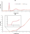 |
Fig. 1 Comparison between the structure modeled through MD simulation in this work (continuous line), and the experimental results from Mariedahl et al. (2018) (dashed line), with (a) RDF for the O-O distance and (b) running coordination number for ASW-LDA ices analogs. |
2.2 ONIOM-2 scheme
The choice of the hybrid ONIOM (our own N-layered Integrated molecular Orbital and Molecular mechanics) scheme (see Svensson et al. 1996; Dapprich et al. 1999; Karadakov & Morokuma 2000; Vreven et al. 2006 and the review from Chung et al. (2015) and references therein) is justified by the large size of the system of interest. Indeed, accurate modeling of binding interactions on ASW requires proper treatment of both long-range and nonlocal effects, especially for hydrogen-bond cooperativity as discussed in, for example, Ferrero et al. (2020). The lack of long-range structural order in ASW, as opposed to crystalline ice, is expected to significantly impact adsorption energetics. To explicitly capture these contributions, the system must therefore be described as extensively as computationally affordable. The use of purely QM methods being consequently proscribed by a too high computational resource requirement, a hybrid/multiscale method has been chosen to handle calculations within a reasonable timescale by splitting the system into multiple fragments. These fragments are then treated using different theoretical methods with distinct levels of theory.
More specifically, an ONIOM-2 approach has been adopted, proven to be suitable in similar study contexts (Duflot et al. 2021; Tinacci et al. 2022); the system is divided into 2 layers, (i) the model system and (ii) the real system, representing the whole system. The ONIOM-2 energy is inferred from Eq. (2).
 (2)
(2)
with EONIOM−2(High:Low) being the extrapolated ONIOM energy, E(real,Low) quantifying the energy of the real system computed at the low-level of theory and E(model,High) & E(model,Low) corresponding to the energy of the model system inferred, respectively, from the chosen high and low-level method.
In the context of this study, ONIOM computations were applied on hemispherical cuts from the MD modeled ice box. These cuts were applied through a custom Python script, ensuring that all water molecules included in a given hemisphere are complete, without cut bond. Using the Gaussian software v. 16 (Frisch et al. 2016), the actual ONIOM scheme consists of an ONIOM-2(B3LYP-D3(BJ)/6-311+G(d,p):GFN2-xtb external program), as justified in the following.
The expression used for the computation of BEs is given by Eq. (3). We note that the BEs are corrected for ΔZPE from harmonic-oscillator frequency computations, and the basis set superposition error (BSSE). The latter accounts for a spurious contribution that comes up in the calculation of interaction energies, leading to an overestimation of the inferred BEs or, in other words, to an over-stabilization of the complex surface-adsorbate. This arises from the use of finite basis sets, and the superposition of the basis set functions of the interacting fragments (here, (i) the adsorbate, and (ii) the ice system, especially around the binding point), effectively increasing the basis set of each component in the complex.
![Mathematical equation: $\begin{align*} B E & =-\Delta E_{{Int}}\\ & =-\left[E_{{complex}}-E_{{ice}}-E_{{ads}}+\Delta E_{C P}^{B S E *}+\Delta Z P E^{*}\right] \\ & =B E_{S C F}+\Delta E_{C P}^{B S E}+\Delta Z P E \\ \text {with}\ & \Delta Z P E^{*}=\left(E_{Z P E, \ {complex}}-E_{Z P E, \ {ice}}-E_{Z P E, \ {ads}}\right) \cdot f_{{scaling}} \\ & =-\Delta Z P E,\end{align*}$](/articles/aa/full_html/2025/06/aa55097-25/aa55097-25-eq3.png) (3)
(3)
where ΔEInt is the interaction energy, Ecomplex is the energy of the complex adsorbate-ice, extrapolated from ONIOM computations (Eq. (2)), Eice is the ice energy, also extrapolated from ONIOM computations, and Eads is the energy of the adsorbate, computed at the high level of theory used for the ONIOM scheme.  is the counterpoise-correction by Boys and Bernardi for the BSSE computed on the model zone; BSSE is actually expected to be nonzero only near the adsorption site. Indeed, regarding the finite size of the used basis set, as the adsorbate approaches the substrate, its basis functions are susceptible to overlap those from water molecule atoms from the surface. This overlap is therefore most likely to occur around the binding site.
  and
and  have opposite signs, typically taking positive and negative values, respectively.
  is the ZPE energy of fragment i (computed under the harmonic oscillator hypothesis), multiplied by fscaling, the frequency scaling factor. This factor depends on both the employed computational method (here, the DFT functional) and the basis set, and is taken from the NIST database2. BESCF stands for the BE values without taking into account the BSSE and ZPE contributions.
2.2.1 Model zone setup
(a) Model zone size. The high-level (HL) size RModel,HL has already been constrained in Tinacci et al. (2022) in similar systems, in which a benchmark on the model zone size on a cluster of 200 water molecules has been performed. In contrast with the ASW model building method in the present study, the cluster in Tinacci et al. (2022) was made through a bottom-up approach, without PBC. In this paper, the BE computation was made onto hemispheric sub-water clusters extracted from the larger ASW analog, taking advantage of the PBC along the x and y axes. This benchmark scanned RModel,HL from 5 to 8.5 Å on eight different optimized binding sites. Results showed that BE slowly evolves with increasing model zone size, showing different evolution tendencies over the studied binding sites, with variations within 5 kJ/mol, or slightly above. In this scope, in order to save computational resources, the smallest RModel,HL, 5 Å, corresponding to the adsorbate plus 3 to 9 H2O depending on the binding sites has been chosen. However, upon closer examination of the results from Tinacci et al. (2022), the BE convergence with regard to the model zone size is located around 7−8 Å, corresponding to 11 to 36 H2O depending on the binding site. Moreover, with regard to the small model zone within the method proposed by Tinacci et al. (2022), system rearrangements forced iterative redefinitions of the water molecules included in the model zone. Consequently, in the scope of this study, RModel,HL was set as a starting point to 8 Å, corresponding to 20−25 water molecules (plus the adsorbate). In other words, all H2O lying within 8 Å from the adsorbate barycenter, without any cut bond, are included in this model zone. This choice is further supported by the study by Duflot et al. (2021), who performed BE computations on hemispheric cuts, with RModel,HL equal to 7−8 Å, including around ∼20 water molecules. Moreover, in Song & Kästner (2016, 2017), the model zone includes all water molecules with at least one atom within 6 Å; that is, 23 H2O, also using a hemispheric cut. This is therefore analogous to the model zone size setup in this work.
It is worth mentioning that, to get a converged result, the choice of RModel,HL depends on the system, including the structure of the ice model, the adsorbate, and the sampled binding site, but also on the real system size and the low-level method, as well as the high-level method. For that reason, the value of 8 Å for the model zone size will be retro-checked downstream the benchmark on the low-level size, discussed in Sect. 2.2.2.
(b) High-level QM method. The model zone is treated under a DFT scheme. More specifically, the hybrid exchangecorrelation B3LYP functional (Lee et al. 1988) along with the D3 version of Grimme’s dispersion correction with the Becke-Johnson damping function (Grimme et al. 2010, 2011) has been used (D3(BJ) in the following), as in Ferrero et al. (2020), in which the BEs of a set of relevant interstellar species were computed through periodic calculations. This choice of functional was based on results in Kraus et al. (2018) in which B3LYP-D3(BJ) has been shown to provide a good level of accuracy for the interaction energy of non-covalently bound dimers, with a mean absolute error of 0.06 Å with regard to semiempirical bond length data.
DFT functional benchmark results with respect to CCSD(T) over the three adsorbate test cases.
The use of this functional has been further validated by means of a benchmark on tetrameric binding configurations, implying three water molecules plus a given adsorbate. Two basis sets are compared, namely 6-311+G(d,p) and aug-cc-pVTZ. In practice, for each studied adsorbate, one tetrameric structure per species is extracted from optimized adsorbate-ice complexes and its isolated counterparts. Subsequent single-point energy evaluations have been performed to infer the interaction energies, including the BSSE contribution (but not the ΔZPE); actually, the BSSE amplitude depends on the chosen basis set, and this dependency itself depends on the level of theory. More specifically, wavefunction-based CCSD(T) is more sensitive to the finite size of the basis set than DFT methods. Using CCSD(T) as reference, results from 8 DFT functionals (B3LYP-D3(BJ); PBE1PBE-D3(BJ); PBE0; BMK-D3(BJ); BMK, B3PW91-D3(BJ); B3PW91; CAM-B3LYP; M06-2X; B97-D3(BJ); B97-D3; ω B97X-D) have been compared with or without dispersion correction depending on their respective parameterization. The performance of each functional relative to the CCSD(T) results varies depending on the studied interaction type and the adsorbate. The main objective pursued in this study is the development of a method applicable to several relevant closed shell interstellar species. Therefore, this benchmark approach has the aim to select a functional that provides an appreciable estimate over different molecular interactions. In this regard, the prime interest is directed toward the mean absolute relative difference (MARD) over the three adsorbates with respect to the CCSD(T) value for each functional, as presented in Table 1. Quantitative details are given in Appendix B. From these results, B3LYP-D3(BJ) provides the best estimations for both basis sets. The relative differences between the 6311+G(d,p) series and the improved aug-cc-pVTZ performances arise primarily from the BSSE correction contribution applied to the reference value. For instance, with the 6-311+G(d,p) basis, in the case of CO, the BSSE CSSD(T) correction (4.2 kJ/mol) approaches the same magnitude as the interaction energy itself (5.6 kJ/mol), underlining the importance of carefully considering BSSE and its own uncertainty when interpreting benchmark results for such systems. Considering the more extended aug-cc-pVTZ basis set, this contribution reduces to 2.2 kJ/mol, for BE value of 8.5 kJ/mol. Given the ultimate goal of extensively sampling an amorphous water surface with relatively large water subclusters, B3LYP-D3(BJ)/6-311+G(d,p) as high-level of theory nevertheless offers a good compromise for an appropriate accuracy/computational cost balance. As final argument in favor of this choice, the convergence between the B3LYP-D3(BJ)/6-311 +G (d,p) and B3LYP-D3(BJ)/aug-cc-pVTZ results is discussed in Appendix C.
2.2.2 Low-level design
(a) Real system size benchmark. So far, very few studies have addressed the impact of the system size, or more specifically the value of the real system size, on the inferred BEs. However, an appropriate choice of the model zone size RModel,HL and of the total system size (RHem,Real=RModel,HL+Δ RLL, LL standing for the low-level of theory) are also of prime importance to obtain convergent BEs. Indeed, as previously stated, to accurately model binding interactions on ASW systems, one should properly take into account the contributions from long-range and nonlocal interactions, with a prime emphasis on H-bond cooperativity (Ferrero et al. 2020). In order to properly include such contributions, the real system size has consequently been benchmarked, with low-level shell size Δ RLL ranging between 3 and 11 Å, resulting in real system size RHem,Real expanding from 11 to 19 Å. We note that, throughout this study, the molecules in the Δ RLL shell are kept frozen. This freezing of the low-level zone has also been applied by Duflot et al. (2021) and Tinacci et al. (2022). This artificially preserves the ice stiffness experienced in real size systems far from the binding zone while reducing the computational cost compared to a flexible low-level zone.
The structure of each of these systems is optimized through ONIOM computations, with the semiempirical GFN2-xtb algorithm from the Grimme’s group (Bannwarth et al. 2019, 2021) as low-level method. These computations are therefore performed at ONIOM(B3LYP-D3/6-311+G(d,p) : GFN2-xtb) level. ΔZPE and BSSE contributions are included. For the model zone, Gaussian16 tight Self-Consistent-Field (SCF) convergence criteria are used. For the low-level treatment, as xtb is not implemented in Gaussian (Frisch et al. 2016), it has been called through the standardized wrapper interface (Beaujean et al. 2021) for communication with external program proposed by Gaussian16, with default SCF parameters. The three adsorbate test cases have been studied at a first binding site, and another binding site has also been studied with NH3. In fact, NH3 is known to present a large BE dispersion compared to CO and CH4. Studying a second binding site with distinct binding behavior is therefore relevant to extrapolate the conclusions for the final sampling of the BE distributions. The results are given in Table 2.
For NH3 on a first site, the BEs are converging from ΔRLL of 8 Å, corresponding to a total radius of 16 Å, at a value of ∼53 kJ/mol. At ΔRLL equal to 6 Å, one underestimates the converged results only by less than 2 kJ/mol, which accounts for less than 4% of the total BE for this case. Regarding CO, the convergence already appears at ΔRLL of 4 Å. On the other hand, CH4 BE values show a slower convergence, appearing only from a ΔRLL of 10 Å, at a BE of ∼10−3−10.5 kJ/mol. A ΔRLL of 8 Å leads to an under-estimation of 0.5−07 kJ/mol (<7%) with respect to that converged value, while a ΔRLL of 6 Å underestimates the converged value by 1.2−1.4 kJ/mol(∼13%). In the case of NH3 at a second binding site, the convergence of the BE value takes place at ΔRLL of 10 Å, at ∼23−23.5 kJ/mol. With ΔRLL of 6−8 Å, one underestimates this converged value only by ∼1 kJ/mol, representing ∼5% of the total value of NH3 BE at this site. Focusing then on the smallest system size, with a ΔRLL of 3 Å, the computed BE drastically increases toward a value of more than 80 kJ/mol. It can be arguably rationalized by geometrical artifacts due to the asymmetry of the extracted hemisphere caused by its small size. The system asymmetry rapidly decreases with increasing system size. Furthermore, one may also suggest a potential too small effective coherence (i.e., rigidity) of the ice system at such a small system size. Indeed, as the low-level zone (frozen) is embedding the model zone, a too small ΔRLL may in some cases not be representative of the embedding environment from a real ice system and its intrinsic H-bond cooperativity, enhancing its coherence.
Taking all these considerations into account, ΔRLL of 8 Å seems to be the best compromise between accuracy and computational cost. It corresponds to ∼210−225 H2O molecules in the ΔRLL frozen ice shell, and therefore a total number of 235–250 water molecules are included in the entire ice hemisphere. This is similar to the system size of Tinacci et al. (2022), in which they used a water cluster of 200 molecules.
Regarding finally the contributions of the applied correction, ΔZPE generally accounts for ∼20−25% of BE, and can go up to 50% for weakly bound systems as in the case of CH4 (apolar). On the BSSE side, their contribution to the inferred BEs is more variable, ranging from 5−10 to 25% depending on the adsorbate and the binding site. We note also that both of these contributions are very stable with respect to the ΔRLL value.
The same benchmarking analyses have been conducted with three other basis sets for the model zone description, namely def2-TVZPP, aug-cc-pVDZ, and aug-cc-pVTZ. This has the aim of quantifying the stability of the computed BEs with growing real system size against different basis set for the high-level. The results are discussed in Appendix C. From a general perspective, across the 3 adsorbate test cases, there is a consistently good match of the results obtained with ONIOM(B3LYP-D3(BJ)/6-311+G(d,p):xtb) and ONIOM(B3LYP-D3(BJ)/aug-cc-pVDZ:xtb) or ONIOM(B3LYP-D3(BJ)/aug-cc-pVTZ:xtb). This indicates that 6-311+G(d,p) is suitable to capture the essential features of the electronic structure relevant to this study.
(b) GFN2-xtb performance for the low-level description. Although the convergence of the BEs with respect to the real system size has been investigated, it is nevertheless worth questioning the reliability of the employed low-level method; that is, the semiempirical GFN2-xTB quantum mechanical algorithm developed by the Grimme group (Bannwarth et al. 2019, 2021). The general performances of GFN2-xtb have already been widely investigated and validated, such as in the original Bannwarth et al. (2019) paper. It has also been evaluated in Germain & Ugliengo (2020) and Tinacci et al. (2022) on similar amorphous water systems than in our context of study. In order to gain additional method-specific insights into the stability of xtb performance against growing ΔRLL, ONIOM2(DFT:xtb) BE results are compared to ONIOM2(DFT:DFT) results with growing real system sizes, as deeply commented in Appendix D. While these results showed an overall good stability of the xtb performances as compared to DFT treatments over growing real system size at BE-real system size convergence, they also provide further justifications for the previously commented choice of the ΔRLL size. These are complementary to the analysis from Germain & Ugliengo (2020) and Tinacci et al. (2022).
2.2.3 Retro-verification of the ONIOM setup (layer sizes)
In order to retro-check the chosen model and real system sizes, taking advantage of the 2D (x−y) PBC of the final box from the MD simulations, computations of BEs are performed on even larger hemispheric cuts, with RHem,Real of 25 Å for a model zone size of 12 Å. BESCF has been recomputed for each of the three adsorbate test cases at the first sampled binding site, in order to compare the results with the converged BESCF values at largest benchmarked real system size, as reported in Table 2. Indeed, this retro-checking is highly resource-consuming; knowing that ΔZPE and BSSE corrections are stable against the system size, these have not been considered in this part of the study.
For NH3, BESCF amounts to 72.8 kJ/mol, only differing by ∼0.9 kJ/mol (less than 1.5%) as compared to the value of 71.9 kJ/mol for the largest studied system size in Table 2. In the case of CH4, a value of 16.9 is obtained from this retro-checking, compared to 16.0 kJ/mol. Therefore, the relative difference accounts for less than 6%. Concerning CO, a value of 15.6 kJ/mol is obtained, in complete agreement with the rapid convergence of the CO BEs with respect to the cluster size at a BE of 15.3 kJ/mol. These results validate the choice of high- and low-level sizes for the ONIOM scheme design.
2.3 Twofold BE sampling
The sampling of the binding sites and starting configurations has been performed through a custom Python script, randomizing the substrate exploration in terms of binding sites and adsorbate-to-substrate orientations. More specifically, the underlying sampling methodology is twofold, distinguishing two main sources of BE diversity: (i) the surface typology and its complexity, itself related to the amorphicity of the underneath ice, and (ii) the substrate-to-adsorbate orientations, and the associated local roughness of the potential energy landscape at a given binding site. The first source can be sampled unbiasedly by placing a regularly spaced grid above the surface to define the starting position of the adsorbate barycenter for subsequent geometrical optimizations. The second source of binding diversity is sampled by considering various adsorbate orientations for each spatially distinct binding site. After geometry optimization, the computed BEs can in fact vary due to distinct optimized configurations4, thereby contributing to the local roughness of the potential energy surface (PES) at each sampling grid point. In other words, a binding zone associated with a given sampling grid point is not a perfectly smooth well within the substrate PES, but rather displays a kind of sub-energy-landscape accounting for different adsorbate-to-substrate optimized configuration. The consideration of this second source of heterogeneity to the energy landscape of an amorphous surface is important to comprehensively sample its diversity. We note that in the method proposed in Tinacci et al. (2022), the adsorbate orientation is randomized, but considering a single orientation per site.
In practice, this custom Python script automates the workflow from the hemispheric cuts in the MD-modeled water box, to the ONIOM-2 input writing within the ONIOM scheme designed upstream the BE sampling, their submission and monitoring. More details on the steps followed by this script are provided in Appendix E. For each binding site, the number of adsorbate-to-substrate starting orientation(s) per adsorbate depends on the adsorbate symmetry; for NH3, three starting orientations have been studied, with (i) the three hydrogens facing the surface, (ii) the three hydrogens flipped in the opposite direction in z , and (iii) the plane formed by the three hydrogens being perpendicular to the surface. In the case of CO, three orientations have also been sampled, with (i) CO axis parallel to the surface, (ii) CO axis parallel to the normal to the surface, with O atom facing the surface, and (iii) the opposite. Finally, because of its higher order symmetry, only one orientation has been studied for CH4.
The binding configuration redundancy reduction deserves further comments. On the one hand, concerning juxtaposed binding sites, the separation distance between points in the sampling grid has been chosen large enough to avoid any redundancy between adjacent sites, minimizing the probability that the NH3 position evolves toward the same energy minimum (same implied water molecules from the surface) as the juxtaposed system during the geometry optimization. A RMSD analysis confirming this point has been performed, as discussed in Appendix F. On the other hand, regarding the case of different starting orientations of the adsorbate on a given hemispheric cut converging toward the same energy minimum, this redundancy has been reduced to the distinct binding configurations per binding site. More precisely, such an in-site redundancy has been identified based on the ΔBE and RMSD values between pairs of starting adsorbate-to-substrate orientations; that is, defining ΔBEij < 0.05. < BE > ij kJ/mol and RMSD <1 Å as redundancy cutoffs, where ⟨BE⟩ij is the mean BE for i and j orientations. Further comments are given in Appendix F. In this idea, the resulting distribution refers to the sampling of each unique trap within the potential energy landscape of the substrate, both in terms of locally distinct sites and local traps.
3 Results – newly inferred distributions versus previously reported values
3.1 NH3 as adsorbate
After geometry optimization and harmonic frequency computation, only 9 geometry optimizations of adsorbate-ice systems out of 300 did not converge under the defined cutoffs, and 25 systems showed imaginary frequencies, of which 14 showed 1–3 imaginary frequencies in the range from i 1 to i 27 cm−1. Because of the small values of these imaginary frequencies, they are not associated with NH3 nuclear motions and do not contribute significantly to the calculation of ZPEs, as justified by Tinacci et al. (2022). Based on these considerations, these 14 systems are also retained. This yielded 280 zero-point and BSSE-corrected BEs for NH3 interactions with the modeled ASW ice analog. After reduction for in-site binding configuration redundancy, the final dataset consists of 204 BE values.
The resulting normalized distribution is given in Fig. 2, on top of which a Gaussian mixture model (GMM, in mauve) is fitted. Indeed, standard Gaussian fits have been tested as well as other nonsymmetric fit types, but it turns out that the data are much better described by this GMM profile. Previously reported single NH3 BE values (vertical lines) or dispersion (horizontal intervals) are also reported.
In terms of distributions, Fig. 2 reports the dispersion from Ferrero et al. (2020) who studied the binding behavior of interstellar species on an ASW model through PBC B3LYP-D3(BJ)//HF-3c composite computations; that is, with geometry optimization with the HF-3c method (Sure & Grimme 2013), and subsequent single point energy evaluation at B3LYP-D3(BJ) level of theory. The resulting NH3 BE distribution ranges from 35.9 to 62.8 kJ/mol. From the amorphous model in Ferrero et al. (2020), made of a unit cell with 60 H2O, only seven binding sites were studied. Moreover, the starting positions were chosen based on electrostatic potential map to maximize the chance of a strong H-bond interactions. As compared to this work, results reported in Ferrero et al. (2020) only cover the range characteristic of the main peak from the GMM fit in Fig. 2. This arguably comes from the lower number of sampled binding sites while biasing the adsorbate position by optimizing the adsorbate surface orientation. All NH3 binding configurations in Ferrero et al. (2020) presented NH3 as acceptor of a H-bond, explaining that no contribution from the lower energy part of the NH3 BE distribution presented here is included in the results reported in Ferrero et al. (2020). The BE dispersion from Duflot et al. (2021) is also given on Fig. 2, where ONIOM(CBS/DLPNO-CCSD(T):PM6)//ONIOM(ω B97X-D/631+G**:PM6) ZPE-corrected BE computations (no BSSE correction) were performed on hemispheric cuts with a model and real system sizes of 8 and 12 to 15 Å, respectively. This resulted in hemispheres including 140 to 170 H2O. The initial positions for a given adsorbate were defined from upstream classical molecular dynamics trajectories at 77 K , modeling the adsorption of single water molecules with a random starting position of the adsorbed water molecules for each trajectory. As compared to the sampling method in the present paper, it intrinsically hinges on the water molecules adsorption behavior at such temperature conditions. This therefore accounts for a more biased sampling of the binding site since water molecules are more likely to reorient and, to a lesser extent diffuse, at 77 K. As compared to the distribution from this work, results in Duflot et al. (2021) cover a much narrower range of energy, with BE values of 35.8 ± 3.4 kJ/mol. The work by Tinacci et al. (2022) has also been considered, a paper extensively discussed upstream due to its similarities with the method adopted in the present paper. Indeed, the method developed in Tinacci et al. (2022) aimed to sample the NH3 BE distribution by unbiasedly defining the adsorbate initial position, while randomizing its orientation with respect to the surface with one random orientation per sampled position. The underneath BE inference method consists of an ONIOM(DLPNO-CCSD(T)//B97D3(BJ):xTB-GFN2) approach, with a model zone of 5 Å including ∼3−10 water molecules. The ASW model was composed of an agglomerated cluster of 200 water molecules built from successive MD additions of H2O and stepwise geometry optimizations. After binding site redundancy reduction, the resulting NH3 BE distribution includes 77 values from the 162 starting points. As compared to results in Ferrero et al. (2020) and Duflot et al. (2021), the distribution in Tinacci et al. (2022) is much wider, leading to a BE dispersion of 31.1 ± 8.8 kJ/mol. This fully covers the low-energy tail from the results presented in this paper, but does not reproduce the higher-energy tail. The methodology proposed in Tinacci et al. (2022) implied the sampling of the full surface of the 200−H2O icy model by projecting a uniformly spread grid of points. In the present paper, hemispheric clusters have been extracted from a larger water box. The aim of this is to ensure that we reach bulk properties below the sampled surface, as well as avoid local edge effects. Moreover, the model zone in Tinacci et al. (2022) was smaller than in this work. The deviations between the results of these works and the results of the present study are probably explained by the number of sampled binding interactions, combined to the chosen sampling grid spacing, and by the study of three adsorbate starting orientations per grid point.
Furthermore, single value references are also given in Fig. 2. The plain gray line represents the BE value found in Ferrero et al. (2020) in which they also studied the binding behavior of interstellar species on a periodic crystalline proton-ordered ice slab model, with a BE value of 51.8 kJ/mol. Although it falls within the BE distribution from this work, it is larger than the mean of the main peak. This trend has also been highlighted in Ferrero et al. (2020). This is simply due to the higher rigidity of the crystalline phase, which enforces the typical binding interactions through a smaller distortion energy cost upon adsorption. Dashed lines report on single BE values from the UMIST/KIDA databases, as well as the computational work by Wakelam et al. (2017), Das et al. (2018) and Penteado et al. (2017) where BE was inferred from the empirical study by Collings et al. (2004). It is interesting to highlight the value found in Penteado et al. (2017), surprisingly falling in the middle of the lower energy subpeak of the distribution reported here. However, this was computed from inversion curves from TPD experiments and greatly depends on the adopted pre-exponential factor.
From an overall perspective, this comparison demonstrates that all single values and energy ranges covered by the previously published NH3 BE distributions are encompassed by the NH3 BE dispersion resulting from the present study. In contrast, none of those previously published distributions individually covers the full range spanned by the results reported here. A combination of these distributions is required to achieve this coverage. It thereby allows for a kind of consensus that could not previously be established as a result of the disparity in the range of energetic values previously covered. Combined with the special attention devoted to the statistical convergence of the inferred distribution (see Sect. 4), compliant with the expectations of improvements from the method presented in this paper, this lends support to the credibility of the newly proposed NH3 BE distribution. Let us nevertheless remind the different levels of theory/method of BE inference among the compared works, and their inherent uncertainty. Moreover, this clearly highlights the significant challenge faced by the astrochemical community regarding the high uncertainty in BEs. The frequent assumption of a single value per adsorbate in chemical networks drastically impacts inferred surface chemistry, as discussed and studied in Grassi et al. (2020). In the case of NH3, given the observed large BE distribution dispersion, its consideration should have a substantial effect on the results of the associated surface chemistry. Furthermore, it is known that in molecular clouds, NH3 is a key component of water-rich icy mantles. Therefore, accurately considering its BE distribution, including the first peak at low BEs , is of paramount importance, as further commented in Sect. 4.4.
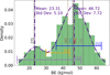 |
Fig. 2 Normalized histogram of sampled NH3 BE (in kJ/mol), fitted with a GMM using scikit-learn algorithm (Pedregosa et al. 2011). Previously reported NH3 BE values onto water ice analogs with diverse simulation methods are given on top. Horizontal intervals report on published BE dispersions, while vertical dashed lines relate to works focusing on single BE values. Methods used in each work are discussed in the text. The BE value on crystalline ice from Ferrero et al. (2020) is also given (plain gray line). Ref: [1] Ferrero et al. (2020); [2] Duflot et al. (2021); [3] Tinacci et al. (2022); [4] UMIST , [5] Wakelam et al. (2017)/KIDA; [6] Das et al. (2018); [7] Penteado et al. (2017); [8] Ferrero et al. (2020) on crystalline ice. |
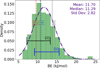 |
Fig. 3 Normalized histogram of sampled BEs (in kJ/mol) for CO, fitted with a single component gaussian profile. Previously reported results of CO BE values onto water ice analogs with diverse simulation methods are given on top. See Fig. 2 for the meaning of horizontal intervals, vertical dashed lines, and the plain gray line. Ref: [1] Ferrero et al. (2020); [2] He et al. (2016) and Penteado et al. (2017); [3] UMIST; [4] Wakelam et al. (2017)/KIDA, [5] Das et al. (2018); [6] Ferrero et al. (2020) on crystalline ice. |
3.2 CO as adsorbate
After geometry optimization and harmonic frequency computation, 19 geometry optimizations of adsorbate/ice systems out of 300 did not converge within the defined cutoffs, and 33 systems exhibited imaginary frequencies, of which 18 configurations showing one to max three imaginary frequencies in the range i3 to i19 cm−1 have been kept. 266 systems have provided valid BE values for the study of CO binding behavior on ASW ices. After reduction for in-site binding configuration redundancy, the final dataset for CO is composed of 228 BE values. The associated normalized distribution is given in Fig. 3, on top of which a Gaussian profile is fitted (mauve). As expected, the mean BE is significantly below the typical values for NH3. This is related to the absence of H-bonding interactions with CO because of its strong internal bonding and the associated electron distribution that prevents it from forming significant H-bonds with water molecules. Previously reported single CO BE values or dispersion are also reported in Fig. 3.
In terms of distributions, results from Ferrero et al. (2020), in which 5 binding sites for CO were sampled, as well as experimental TPD results from He et al. (2016) and Penteado et al. (2017) have been considered. Both of them mostly cover the central part of the distribution reported in this work, but none includes the left and right tails. This is certainly explained by the higher number of sampled binding sites as well as the systematic study of multiple starting adsorbate orientations in the method proposed in the present work. This is supported by the great attention devoted to the converged nature of the inferred distribution, and the associated difficulty to accurately reproduce the slowly converging standard deviation (see Sect. 4).
Regarding previously published single values for CO, the crystalline CO BE from Ferrero et al. (2020) (plain grain line) falls to the mid-high side of our distribution, a trend also emerging from the analysis of the NH3 distribution, as well as from the results in Ferrero et al. (2020). Dashed lines concern single BE values from the UMIST/KIDA databases, as well as from the computational work from Wakelam et al. (2017) and Das et al. (2018), all of them falling within the energy range covered in this work, slightly below the computed global mean and median. As for NH3, this comparison showed that the newly proposed results encompass both the previously reported unique values and distributions, while previously published BE dispersion does not cover on their own the CO BE distribution reported here.
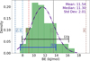 |
Fig. 4 Normalized histogram of sampled BEs (in kJ/mol) for CH4, fitted with a single component Gaussian profile. Previously reported results of CH4 BE values onto water ice analogs are given on top. See Fig. 2 for the meaning of horizontal intervals, vertical dashed lines, and the plain gray line. Ref: [1] Ferrero et al. (2020); [2] Smith et al. (1989), He et al. (2016), and Penteado et al. (2017); [3] UMIST; [4] KIDA, [5] Wakelam et al. (2017); [6] Das et al. (2018); [7] Ferrero et al. (2020) on crystalline ice. |
3.3 CH4 as adsorbate
In the case of CH4, only one starting orientation per cut has been studied. Out of the 100 starting CH4/ice systems, all converged and six of them showed imaginary frequencies, among which four presenting two to a maximum of three imaginary frequencies in the range from i2 to i16 cm−1 have been kept for the statistical analysis. Consequently, 98 CH4 BEs energies have been successfully computed for the sampling of CH4 BE distribution. The normalized BE distribution is shown in Fig. 4. The mean and median are sensibly close to CO-related values. However, the standard deviation is lower, with a reduced upper limit as compared to CO. This is attributed to the apolarity of CH4. Previously reported single CH4 BE values or dispersion are also reported in Fig. 4.
In terms of distributions, the work from Ferrero et al. (2020), in which five binding sites were tested, is still considered, as well as the experimental TPD results by Smith et al. (1989), He et al. (2016) and Penteado et al. (2017). Both are included in the CH4 BE range reported in this work, and the experimental values cover more than 90%. However, one should keep in mind that the BE value inferred from TPD experiments greatly depends on the adopted pre-exponential factor for the inversion method. Concerning single values, the KIDA and UMIST references fall in the low-energy part of the distribution from the present work, while the crystalline BE value of Ferrero et al. (2020) lies in the middle-to-high energy range of our results, as expected. On the other hand, the values of Wakelam et al. (2017) and Das et al. (2018) are outside the range of the newly reported distribution. This is probably explained by the size of the water ice model: a single water molecule in Wakelam et al. (2017) and a cluster made of up to 6 H2O in Das et al. (2018). Such small water systems are not adequately accounting for the converged nature of BEs relative to the size of the ice model, underestimating the ice rigidity, long-range forces and H-bond cooperativity. Together with the convergence analysis presented in Sect. 4, these results are therefore consistent.
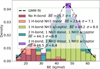 |
Fig. 5 Statistical analysis of subgroup contributions using stacked histograms normalized on the global BE distribution for NH3, each subgroups representing a type of adsorbate-ice H-bond configuration. |

4 Further discussions
4.1 Geometrical and molecular surrounding insights
(a) NH3 binding behavior. The inferred NH3 BE distribution displays a bimodal profile. Actually, NH3 is able of forming H-bonds with water, acting as both a donor and an acceptor. More specifically, NH3 is a strong H-bond acceptor, due to the high electron density in the nitrogen lone pair. However, the NH3 H-bond donation capabilities lead to weaker H-bond due to the relatively low polarity of the N-H bond compared to, for example, the highly polar O−H bond in water. As a comparative reference, BEs on H2O−NH3 dimers at CCSD(T)/aug-cc-pVTZ level amount to 27.0 and 9.5 kJ/mol for NH3 acting as acceptor and donor, respectively, to be compared to 29.7 kJ/mol for H2- H2OH-bonding interaction. With NH3 approaching the surface with different orientations, the binding interactions result in 0 to 3 H-bonds with the underlying water molecules. The case with 4 H-bonds would only be possible if cavity-like binding sites were studied, which is not the case in this paper.
To gain insight into the link between the BE and the number of H-bonds, a statistical analysis of the contributions of subgroups using stacked histograms normalized onto the global NH3 BE distribution has been performed using a custom Python script, as presented in Fig. 5. Each subgroup is distinguished on the basis of the detailed number of H-bonds; that is, the number of H-bonds with NH3 as donor (D) or acceptor (A). The H-bond identification, made from a custom Python script, is based on purely geometrical cutoffs, with a higher limit onto the distance between heteroatoms fixed at 3.2 Å, and a lower limit for the D-H−A angle defined at 140∘. From these results, it appears that the small, left-shifted first peak in the overall distribution is mostly populated by binding configurations implying no H-bond or, at a lower degree, 1 H-bond with NH3 as donor. This is explained by the main implication of nondirectional van der Waals interactions, while the other binding configurations imply hydrogen bonding interactions exhibiting a strong directionality as well as a good cooperative property, typically leading to larger BEs. In fact, the dominant contributions to the major peak of the overall distribution come from binding interactions that display at least one H-bond with NH3 as the acceptor. It is also interesting to note that the contributions from cases presenting H-bonding interactions implying only NH3 as donor are very weak. These results are explained by the afore-discussed NH3 H-bonding donation and receiving capabilities. This is further reflected in the mean distance between heteroatoms, being 2.78 Å ± 0.05 Å for NH3 acting as acceptor, while it amounts to 3.03 Å ± 0.24 Å when it acts as donor.
The results of this clustering analysis partially align with the machine learning (ML) clustering analysis performed in Tinacci et al. (2022), in which the Scikit-learn (Pedregosa et al. 2011) implementation of hierarchical agglomerative clustering was used, with a predefined number of two clusters, using the unreduced BE distribution, the associated electronic BE, the deformation energies, the minimum H-bond distances, and the corresponding angles. This showed that the global distribution can be divided into two sub-distributions with distinct features; weaker adsorption sites are attributed to NH3 acting as H bond donor, while the stronger binding cases to configurations with NH3 as acceptor. The first peak, highlighted through the ML-clustering approach, is, however, less pronounced, and is dominated by configurations presenting NH3 as H-bond donor, while the present analysis rather attributes a clear dominance of configurations without any H-bonding interactions. These deviations in the attribution of the characteristic first peak binding features is arguably rationalized by different geometrical cutoffs used for the H-bond identification, as reflected in the typical Hbond angles for H-bond donation configurations (typically lower than 120∘, with a min N−H distance between 2.5 and 3.5 Å) in results from Tinacci et al. (2022). While hydrogen bonding plays a central role, BE values are likely the result of a intricate interplay of multiple factors, including for instance the local number and proximity of surrounding water molecules, leading to a complex and system-specific energetic behavior.
(b) CO binding behavior. In the case of CO, with the aim of searching for angle-dependent binding behaviors, the orientation of the CO molecule with respect to the reference z-axis has been evaluated by calculating the angle, θ, between the molecular axis (C–O vector) and the z reference unit vector. This angle was obtained using the arc-cosine of the normalized dot product between the C–O bond axis and the z-reference vector, yielding values between 0∘ and 180∘. The resulting angle provides insight into the molecular orientation relative to the surface normal, neglecting the substrate roughness; a value of 0∘ or 180∘ indicates perfect alignment of the CO axis along the z-direction, respectively, with the carbon or oxygen atom pointing toward the substrate. The intermediate case concerns CO axis perpendicular to the z direction and, therefore, mostly parallel to the substrate surface. As for NH3, a supervised clustering approach has been implemented through a dedicated custom Python script, this time discriminating the sub-distributions in terms of θ values. The analysis of subgroup contributions using stacked histograms normalized onto the global CO BE distribution is presented in Fig. 6. From these results, it first appears that very few binding configurations involve very low θ values (0 to 36∘), with the CO axis pointing upward. Furthermore, such CO orientations only cover a narrow low BE range, approximately from 9 to 11 kJ/mol. This suggests that the perpendicular orientation of CO, with the carbon atom facing the surface, results in weaker binding interactions. A slightly higher probability is found for θ to lie in the 36−72∘ range, covering a wider range of BE values. The dominant contributions come from intermediate θ values (72−108∘), although contributions from θ between 108 and 144∘ are also significant. Actually, while this subgroup contribution analysis does not lead to strongly differentiated clustering patterns for the different CO orientations, this highlights the proneness of CO to align with the surface. Beside the adsorbate-to-substrate orientation, multiple other factors are expected modulate the computed BEs via intertwined contributions, likely explaining the large coverage of the total CO BE dispersion for those dominant intermediate θ values. We note also that the highest energy tail of the distribution, from ∼15 kJ/mol, is mostly populated by configurations presenting θ values in the range [108–144∘]. This indicates a slight tendency toward stronger interactions for CO configurations where its axis is inclined, pointing the oxygen atoms toward the surface. This is arguably explained by the electronic density and polarity characteristic of the CO bond, with a small dipole moment and partial charges such as the computed CHELPG charges for the isolated CO molecules are +0.017 and −0.017 for the C and O atoms, respectively. In binding configurations that include θ values in the range [108–144∘], the charges are redistributed with qC ∈ [+0.035, +0.255]; qo ∈ [−0.020, −0.180], with oxygen interacting favorably with partially positive regions (hydrogens, with computed CHELPG charges qH ∈ [+0.200− +0.550]) from the substrate water molecules. Indeed, ASW surfaces exhibit numerous dangling hydrogens. Very high θ values (144−180∘) have a lower occurrence than intermediate cases, only covering BE ranges from the lower two first thirds of the distribution. This suggests that a situation where oxygen is almost totally pointing downward is less favorable, arguably because of the repulsion effect with the oxygen from the surface.
(c) CH4 weak-binding case. Although CH4 exhibits a relatively high isotropic polarizability (2.12 Å3) as compared to NH3(1.72 Å3) and CO(1.75 Å3), the absence of permanent dipole moment and the negligible electronegativity difference between carbon and hydrogen leads to nondirectional dispersiondominated weak interactions with the substrate. This therefore precludes the search of any unambiguous configurational trend that meaningfully correlates with the BEs.
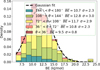 |
Fig. 6 Subgroup contributions of θ value ranges using stacked histograms normalized on the global BE distribution for CO. |

4.2 Analysis of the contributions from ΔZPE
The computation of the ZPE corrections to the BEs is computationally demanding. Nevertheless, this correction contributes non negligibly to the final inferred BEs. In order to find a robust method to avoid these computations, in line with previous works on the BE distribution of interstellar species on amorphous ices, BESCF values are compared to the ZPE-corrected BEs. Fig. 7 provides the corresponding linear correlation for the three adsorbate test cases. The origin has been forced to be equal to 0 to align with previously published results and be able to make rigorous comparisons.
The linear correlation for NH3 is represented by BEZPE−corrected = 0.835 BESCF(R = 0.99). In Germain & Ugliengo (2020), where NH3 BE distribution has been evaluated at full GFN2-xtb level on the same agglomerated cluster of 200 H2O water molecules as in the already largely discussed downstream work by Tinacci et al. (2022), a scaling factor of 0.83 (R = 0.98) is found, which is pretty close to the above results. On the other hand, in the periodic framework followed in Ferrero et al. (2020), this regression has also been studied, but using results for several adsorbates on crystalline ice. This leads to a scaling factor of 0.854. This scaling factor has then been applied to the amorphous systems in order to avoid the related resource-demanding ZPE frequency computations on their larger unit cell, representing the amorphous system.
In the case of CO, the linear correlation between ZPE-corrected BE values and BESCF demonstrates a very appreciable fit, yielding a scaling factor of 0.865 compared to 0.835 for NH3, thus indicating a 3% difference. Regarding finally CH4, the scaling factor is reduced to 0.824 , to be compared to 0.835 and 0.865 for NH3 and CO , respectively.
The three values are of the same order of magnitude over the three adsorbate test cases, and those three adsorbates are sufficiently different to be representative of the various typical physisorption interactions an adsorbate can involve when binded onto such a surface. It is therefore relevant to consider a universal value for the ΔZPE scaling factor, applicable to any adsorbate. This approach will align the method in Ferrero et al. (2020), though directly applied to the computed frequency data for the amorphous ice model, rather than extrapolated from the crystalline phase. In this context, different methods can be arguably adopted. Firstly, the linear fit between ZPE-corrected BEs and the electronic values including the data for all the three tested adsorbates gives a scaling factor of 0.837. This value is not surprisingly closer to the value from NH3 case since it covers a larger range of BEs. Furthermore, in order to give an equal weighting factor for each adsorbate test case, another approach would be to consider the average of the three values specific to each species, leading to a value of 0.841.
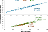 |
Fig. 7 Linear correlation between the electronic BEs and the ZPE corrected values (best fit – dashed line) for NH3 (blue), CO (green) and CH4 (orange) on ASW ice. |
4.3 Convergence analyses
The method built throughout this paper is focused toward the unbiased sampling of statistically converged BE distributions. A rigorous convergence analysis would therefore allow us to objectively comment on the convergence behavior of the datasets. Such an analysis has never been applied in the aforementioned previously published works. In that context, a bootstrapping approach has been applied to assess the convergence of the BE distribution statistics with increasing set sizes of binding configurations. For each of the underlying random samplings of the full set, no repetition was allowed. For each set size, 100 bootstrapping sampling runs were performed.
(a) Sampling of the NH3 mixed gaussian BE profile. Fig. 8 shows the results of such an analysis on NH3 GMM two-component statistics for increasing set sizes, replicating three times the bootstrapping method. The set size was sequentially defined for the three runs by increasing the number of selected adsorbate orientation(s) per cut until all of them are considered. More specifically, for the first run, a single BE value corresponding to a given starting adsorbate-to-substrate orientation was randomly chosen out of the three studied. For the second run, the BE values from two most diverging starting adsorbate-to-substrate orientations (see Sect. 2) were considered, while all the three orientations per cut were included in the last run. At each bootstrapping cycle, for each sampled cut, a binding configuration redundancy analysis was performed when the number of adsorbate orientations considered per cut was greater than or equal to 2.
From the last bootstrapping run including all the three adsorbate orientations per randomly chosen cut, the statistics of both Gaussian components converged, at least within the convergence criteria; that is, with a convergence cutoff tolerance interval of 5% around the mean and standard deviation of the entire distribution. More precisely, convergence is more slowly reached for the low-energy first Gaussian component, intrinsically due to its lower mean and standard deviations, as well as its lower intensity. This is especially true for the standard deviation, with more than 85 cuts required to statistically fall within the defined convergence cutoff. When the number of adsorbate orientations per cut is also considered, increasing the number of starting adsorbate orientations per cut decreases the number of required cuts to reach convergence. Specifically, if only a single orientation per cut is examined, except for the mean for the second and dominant Gaussian component whose convergence is rapid, 100 cuts are insufficient to achieve 5% accuracy around the standard deviation of this main peak. They are also inadequate for reaching similar precision in both the mean and standard deviation of the first component of the GMM fit. By increasing the number of initial orientations per cut to two, convergence is reached for the second dominant peak, yet remains unmet for the low-energy first peak, especially in terms of standard deviation. Robust convergence of the statistics of the first peak, is only achieved by considering three orientations per cut.
(b) CO BE dispersion. The bootstrapping analysis discussed above has been applied to the global mean and standard deviation for sets with increasing set sizes, considering insite binding configuration redundancy reduction. The results are given in Fig. 9. Starting with the rightmost bootstrapping run, including all three geometries per sampled cut, the results indicate converged global statistics, with the mean naturally converging faster than its standard deviation due to the very small magnitude of the latter. To achieve convergence for both within the defined cutoff, a set size of at least 80 cuts is required. However, the convergence criterion for the standard deviation could be slightly relaxed, depending on the desired level of precision. On the other hand, similar to NH3, increasing the number of considered adsorbate orientations per cut leads to faster convergence in terms of cuts, resulting in greater standard deviation stability. Although the convergence (within the defined criterion) of the standard deviation is not reached when only one adsorbate orientation is randomly chosen per cut, it is almost reached after 100 cuts when the two most differing starting adsorbate geometries are considered. However, as was just stated, the very low value of the standard deviation intrinsically results in slower convergence. To optimize the accuracy-computational cost balance based on the convergence of global statistics, studying the two most diverging orientations of CO per cut could consequently be sufficient, once again depending on the level of precision one expects to reach.
(c) CH4 BE dispersion. Results are given in Fig. 10. Despite the lower number of sampled binding configurations due to the single starting orientation of CHr esults 4 , the convergence appears to be well attained under the consideration of at least 85 cuts. The sampling of a larger surface area is thereby not required.
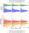 |
Fig. 8 Bootstrapping analysis of GMM two components statistics of NH3 BE distribution, with increasing set size. The set size definition depends on the number of picked adsorbate orientation per cut, increasing from 1 to 3 from the left to the right. The dashed line represents the statistics for the full set of data, while the continuous lines encompass a tolerance interval of 5% around these statistics. |
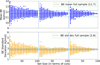 |
Fig. 9 Bootstrapping analysis of mean BE and standard deviation of CO on LDA ice, with increasing set size. The set size definition depends on the number of picked adsorbate orientation per cut, increasing from 1 to 3 from the left to the right. |
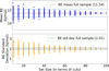 |
Fig. 10 Bootstrapping analysis of mean BE and standard deviation of CH4 on LDA ice, with increasing set size. The set size is defined by the number of picked random hemispherical systems. |
4.4 Astrochemical implications
The three adsorbate test cases were chosen for their distinctive typical interactions with water surfaces, as well as their significance in interstellar ices. In addition to water, CO, NH3 and CH4 are among the main components of such interstellar water-rich ices (Hama & Watanabe 2013; Oberg 2016). Thoroughly studying their BE distribution is, therefore, necessary for an accurate kinetic modeling. In the case of NH3, the double-Gaussian profile is anticipated to have a non-negligible impact on the solid-phase chemistry of cold molecular clouds, where weak binding configurations may enable surface diffusion/desorption, whereas stronger binding cases inhibit it. Actually, as discussed in Sipilä et al. (2019); Tinacci et al. (2022), the gaseous abundance of ammonia in cold prestellar clouds (Crapsi et al. 2007), for instance the L1544 prestellar core, cannot be attributed to the gas-phase chemistry. In fact, NH3 is expected to be completely frozen out in icy matrix in typical prestellar core temperatures; that is, 7 K in the deep interior of L1544 (Crapsi et al. 2007; Keto & Caselli 2010). However, Sipilä et al. (2019) found that a chemical desorption of less than 1% of the NH3 formed on dust grains is sufficient to reproduce the gas-phase abundances measured in L1544. In that context, they explored the possibility that the ammonia BE is lower than the typically considered high value (45.7 kJ/mol), and therefore tested BE values of 24.9 kJ/mol, as suggested in Kamp et al. (2017), and references therein, as well as an ad hoc very low value of 8.3 kJ/mol. The latter led to an overestimation of the ammonia gas phase abundance by orders of magnitude. However, as commented in Tinacci et al. (2022), considering the inferred BE distribution rather than a single BE value may improve the agreement with the observed gas-phase ammonia abundance. Quantitatively, the first peak of the NH3 BE distribution reported in this work, spanning BE range between ∼15 and 30 kJ/mol, covers 16.3% of the total distribution. This suggests a chemical desorption efficiency even lower than the upper limit of 1% proposed in Sipilä et al. (2019). However, as discussed in Sipilä et al. (2019), the gas-phase abundance of NH3 in such a prestellar core may also be arguably explained by the late freezing out of CO molecules in the deep interior of the cloud. This alters the ice composition and arguably decreases the NH3 depletion degree due to weaker binding interactions with the CO-dominated ice. This is still a matter of debate, with the layering of the ice featuring an uppermost CO apolar ice in the late evolution of molecular clouds (Öberg et al. 2011) being contested by the models in Kouchi et al. (2021b,a). If the layering process is effective, we suggest that a mix of both the first BE peak in the NH3 BE distribution on ASW with weak chemical desorption efficiency, coupled with the change of the ice composition at late cloud evolutionary stages, is likely explaining the gasphase abundance of ammonia in a prestellar core such as L1544. Further modeling is needed to verify this suggestion.
5 Conclusions
In this paper, we have presented a revised methodology for the BE distribution inference of interstellar species present in the water-rich amorphous icy mantle in dense clouds and young protostellar cores, using NH3, CO, and CH4 as adsorbate test cases. This methodology relies on the following key points:
The structural reliability of the MD-modeled ASW ice analog, validated through comparisons to previously reported structural data;
The design of the applied ONIOM-2 scheme for the BE computation aiming to be applicable to a wide range of interstellar species. It involves several confirmation steps, with
- (a)
a benchmark on the DFT functional for the description of the model zone. Using CCSD(T) as a reference, B3LYP-D3(BJ)/6-311 +G (d,p) stands out as being the best accuracy-to-computational needs balance;
- (b)
a convergence analysis of the real system size effect on the computed BE values, using GFN2-xtb for the low-level method and a model zone size of 8 Å. This showed that the influence of the real system size depends on the adsorbate as well as the binding site. Over the three adsorbate test cases, a real system size of 16 Å provides the best compromise. This analysis also demonstrated that a real system size that is too low may lead to artifacts in the inferred BE values;
- (c)
an analysis of the GFN2-xtb performances (with respect to a DFT-based treatment) under growing real system sizes, showing that GNF2-xtb is suitable for this study, at least within the chosen real system size of 16 Å;
- (d)
a final retro-verification of the size of the ONIOM layers, confirming the choice of a model zone of 8 Å within a real system of 16 Å.
- (a)
A twofold binding configuration sampling, exploring the diversity in terms of both locally distinct binding sites and the local roughness of the PES. The first source of diversity was sampled through the use of a regularly spaced sampling grid above the surface, defining the position of the adsorbate barycenter. On the other hand, the local roughness of the PES was studied by using multiple starting adsorbate-to-substrate orientations for each binding site. The number of starting orientations was defined by the adsorbate symmetry. This sampling method was designed to ensure the statistical convergence of the inferred BE distributions, as proven through bootstrapping convergence analysis onto the respective mean and standard deviation of the BE distributions.
For some perspective, the method presented in this paper is expected to be applied to other adsorbates relevant to the interstellar medium. The primary focus should be on CO2, H2CO, and CH3OH which are other important constituents of molecular clouds and young protostellar ices (Hama & Watanabe 2013). Furthermore, the impact of the ASW model density on the resulting BE distributions will be the subject of a subsequent paper.
Acknowledgements
We thank the anonymous referee for his/her time, and for his/her fair and positive report. M. Groyne thank the Belgian National Fund For Scientific Research (F.R.S.-FNRS) for the Research Fellow fellowship. These computations were performed on the computers of the “Consortium des Équipements de Calcul Intensif (CÉCI)” (https://www.ceci-hpc.be), including those of the “UNamur Technological Platform of High-Performance Computing (PTCI)” (https://www.ptci.unamur.be) and those of the Tier-1 supercomputer of the Fédération Wallonie-Bruxelles, for which we gratefully acknowledge the financial support from the FRS-FNRS, the Walloon Region, and the University of Namur (Conventions Nos. U.G006.15, U.G018.19, U.G011.22, RW1610468, RW/GEQ2016, RW1117545, and RW2110213).
Appendix A Ice model – Further validation of the structural reliability
A broader comparison has been made to other MD simulations (Michoulier et al. 2018) and experimental results (Narten et al. 1976; Finney et al. 2002; Mariedahl et al. 2018) to address all pairs’ distribution functions. The results are given in Fig. A.1. From a general point of view, the simulated ices of Michoulier et al. (2018) and this work agree very well. Moreover, the modeled data from Michoulier et al. (2018) display the same small qualitative differences discussed above with respect to the experimental curves as our simulations. This match is fairly appreciable despite the different MD simulation protocols, where Michoulier et al. (2018) modeled their ASW ice analogs from conversion of crystalline water ice. This provides a robust warranty to the aforementioned comment on the expected negligible impact of the ice building protocol on the overall structure of the ice model and subsequent inferred BEs.
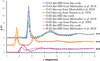 |
Fig. A.1 Intermolecular O–O, O–H and H–H RDFs from this work, Mariedahl et al. (2018) and Michoulier et al. (2018) (with Narten et al. 1976 and Finney et al. 2002 data used in Michoulier et al. 2018). |
We also checked the number of H-bonds per water molecules. This can be studied from (i) the gO−H(r), in combination to its integrated form nO−H(r), or (ii) through analysis of the mean number of H-bonds per water molecule/oxygen atom, as provided by the VMD (alpha 1.9.4 version) visualization and analysis software (Humphrey et al. 1996). nO−H(r) and nO–O(r) display a clear plateau at 3.96–4 in the distance range corresponding respectively to the inter-molecular gO−H(r) and gO−O(r) first peak. This further highlights the almost perfect tetrahedrality of the H-bond network. Concerning the mean number of H-bonds per water molecule, it amounts to 3.97, tending toward the net value of 4 in crystalline water ice.
These results are fully consistent with the discussion in the main text and in line with theoretical considerations. This further validates the suitability of the use of the TIP4P/2005 Force Field in our scheme.
Appendix B Benchmark onto the DFT functional for the model system description – detailed results
Fig. B.1 provides detailed results for the DFT functional benchmark for the model zone description. Results obtained with 6-311+G(d,p) are represented in orange, while blue results stand for QM schemes with the extended correlation-consistent aug-cc-pVTZ as basis set. The first three raws gives results for each adsorbate, while the last raw compares the MARD with respect to CCSD(T) over the three adsorbate test cases. As we can see, the tendencies obtained with 6-311+G(d,p) as basis set are qualitatively retrieved with aug-cc-pVTZ, harboring reduced discrepancies with respect to CCSD(T) values. This is principally due to the magnitude of the BSSE correction onto the reference value, lowered in the case of the aug-cc-pVTZ basis set and its additional diffuse and polarization functions. These diffuse functions are associated with small exponents extending over a much larger spatial domain. Their spatial extension leads to weak overlapping with many other basis functions, introducing very small eigenvalue to the overlap matrix slowing down the SCF convergence. Considering our ultimate goal to extensively sample an amorphous surface, with a relatively large ice substrate (see Sect. 2.2.2), B3LYP-D3(BJ)/6-311+G(d,p) level of theory offers the best compromise for a proper accuracy/computational cost balance for the Model zone treatment. The choice of 6-311+G(d,p) as high-level basis set is further validated in Appendix C.
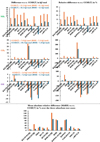 |
Fig. B.1 DFT-functional benchmark on the tetrameric structures; orange and blue series account respectively for results with 6-311+G(d,p) and aug-cc-pVTZ as basis set – left column: difference with respect to CCSD(T) value. CCSD(T) reference BE and BSSE correction values are given explicitly; right column: relative difference with respect to CCSD(T) value in%. Graphs are going by pairs (raw), with the first raw being attributed to NH3, the second to CO and the third to CH4. The last raw gives the MARDs over the three adsorbates. |
Appendix C Stability of the benchmark on the real system size under extended high-level basis set
In order to check the stability of the benchmark results on the real system size under extended high level basis sets, results obtained within an ONIOM(B3LYP-D3(BJ)/6-311+G(d,p):xtb) framework are compared to results obtained with three other basis sets for the model zone description; that is, def2-TZVPP, aug-cc-pVDZ and aug-cc-pVTZ. Results are gathered in Fig. C.1, C.2, C.3 and C.4 respectively for NH3, CO and CH4 on the first binding site, and NH3 on the second binding site.
In the case of NH3, focusing on the middle panel of Fig. C.1, the convergence between BEs and the real system size arises, for each series, from a ΔRLowLevel of 8 Å. In the case of Fig. C.4, every BE series also display consistent convergence trend with respect to the real system size, rather appearing at 10 Å but already appreciable from ΔRLowLevel of 6−8 Å. In terms of ΔBE with respect to the results obtained with a model system treatment at B3LYP-D3(BJ)/aug-cc-pVTZ high level of theory at the largest real system size, these are relatively weak and very stable at system size-BE convergence for the first NH3 binding site, as seen in the bottom panel from Fig. C.1. In the case of the second site, the bottom panel of Fig. C.4 shows that, at ΔRLowLevel in the 6–8 Å range, the ONIOM(B3LYP-D3(BJ)/aug-cc-pVTZ:xtb) result at largest system size is best represented by the ONIOM(B3LYP-D3(BJ)/6-311+G(d,p):xtb). Increasing ΔRLowLevel further, the difference between ONIOM(B3LYP-D3(BJ)/aug-cc-pVTZ:xtb) and ONIOM(B3LYP-D3(BJ)/6311+G(d,p): xtb) increases to ∼5%. These results for the two tested binding sites of NH3 therefore reinforce our choice for the real system size, with ΔRLowLevel equal to 8 Å.
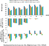 |
Fig. C.1 (top panel) NH3 BEs on a first tested binding site for a growing ΔRLowLevel, going from 3 to 11 Å, for a total radius between 11 and 19 Å. 4 different basis set for the high-level treatment are tested, as given in the legend of the plot, within an ONIOM(B3LYP-D3(BJ)/basis set:xtb) framework; (middle panel) Relative BE difference with respect to BE at ΔRLowLevel equal to 11 Å, each series being treated independently; and (bottom panel) Relative BE discrepancies relative to BE at B3LYP-D3(BJ)/aug-cc-pVTZ high level of theory, with ΔRLowLevel equal to 11 Å. |
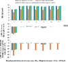 |
Fig. C.2 CO BEs on a first tested binding site for a growing ΔRLowLevel, going from 3 to 11 Å, for a total radius between 11 and 19 Å. Four different basis set for the high-level treatment are tested, as given in the legend of the plot, within an ONIOM(B3LYP-D3(BJ)/basis set:xtb) framework. See legend Fig. C.1 for the description of each panel. |
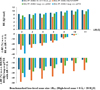 |
Fig. C.3 CH4 BEs on a first tested binding site for a growing ΔRLowLevel, going from 3 to 11 Å, for a total radius between 11 and 19 Å. Four different basis set for the high-level treatment are tested, as given in the legend of the plot, within an ONIOM(B3LYP-D3(BJ)/basis set:xtb) framework. See legend Fig. C.1 for the description of each panel. |
In the case of CO and CH4, the convergence between the real system size and the BE values is also consistent among the different series. In terms of ΔBE relative to model system treatment at B3LYP-D3(BJ)/aug-cc-pVTZ high level of theory at the largest real system size, def2-TZVPP provides results with larger deviations as compared to results with 6-311+G(d,p), aug-cc-pVDZ and aug-cc-pVTZ as high-level basis set. This is likely explained by the absence of diffuse functions in def2-TZVPP, required in the context of the description of the model zone, especially for the weak interaction involved in CO and CH4 binding behaviors. More specifically, at system size-BE convergence, the converged BE value with aug-cc-pVTZ as high-level basis set is best matched by results with 6-311+G(d,p) as high-level basis set, with relative discrepancies lower than 10% for CH4 and 5% for CO.
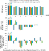 |
Fig. C.4 NH3 BEs on a second tested binding site for a growing ΔRLowLevel, going from 3 to 11 Å, for a total radius between 11 and 19 Å. Four different basis set for the high-level treatment are tested, as given in the legend of the plot, within an ONIOM(B3LYP-D3(BJ)/basis set:xtb) framework. See legend Fig. C.1 for the description of each panel. |
From an overall point of view, one therefore gets consistent conclusions in terms of convergence between the real system size and the inferred BEs for the different high-level ONIOM frameworks over the three adsorbate test cases. At convergence, we observed an overall good match of the results obtained with ONIOM(B3LYP-D3(BJ)/6-311+G(d,p):xtb) and ONIOM(B3LYP-D3(BJ)/aug-cc-pVTZ:xtb), with systematic additional diffuse and polarization functions for the correlation-consistent aug-cc-pVTZ basis set, recognized as particularly relevant in weakly interacting systems. This indicates that 6-311+G(d,p) is suitable to capture the essential electronic structure features relevant to this study and constitutes the final foundation for the applied high level of theory; that is, B3LYP-D3(BJ)/6-111+G(d,p).
Appendix D GFN2-xtb performance for the low-level description – stability of the performance against growing real system size
While the convergence of the BEs against the real system size has been studied, it is nevertheless worth to question the reliability of the used low-level method, namely the semiempirical quantum mechanical GFN2-xtb algorithm from the Grimme group (Bannwarth et al. 2019, 2021), as well as the stability of this reliability itself under growing real system sizes. For that purpose, BEs (corrected for ΔZPE and BSSE) from ONIOM(B3LYP-D3/6-311+G(d,p) : GFN2-xtb) are compared to results from ONIOM(B3LYP-D3/6-311+G(d,p): B3LYP-D3/ growing basis set) for each of the three adsorbate test cases on the firstly studied binding site, with growing hemisphere radius. The tested low-level basis sets correspond to 6-31G, 6-31G(d), 6-31G(d,p), 6−31+G and 6−31+G(d).
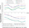 |
Fig. D.1 Top panel – NH3 BE for a growing ΔRLL and various low-levels of theory. The different series hold for a computational scheme following ONIOM(B3LYP-D3/6-311+G(d,p): x), where x , the low-level method, accounts for either for B3LYP-D3/growing basis set (see legend), or GFN2-xtb; Bottom panel – residue graph representing the relative difference between ONIOM(B3LYP-D3/6-311+G(d,p):GFN2-xtb) and ONIOM(B3LYP-D3/6-311+G(d,p): B3LYP-D3/growing basis set). Note that legends only explicit the low-level method of each series, for the sake of clarity. Lines do not represent any interpolated physical trends, they only serve as guides to highlight the trend and facilitate the reader view of the plots. |
In the case of NH3 (Fig. D.1), BE values globally converge in each series from ΔRLL of 8 Å, as does the ONIOM(B3LYP-D3/6-311+G(d,p):GFN2-xtb) series alone. The convergence of the series with a low-level treatment at B3LYP-D3(BJ)/6-31+G and B3LYP-D3(BJ)/6-31+G(d) is less pronounced but still appreciable, with a maximum deviation of 1.5 kJ/mol for values of ΔRLL between 8 and 11 Å. The observed BE oscillations in this ΔRLL range are arguably due to geometrical artifact at the hemisphere boundaries, but no reason has been found to explain the absence of this effect in the other series, or for CO-related series (see Fig. D.2). Concerning the ΔBE between ONIOM(B3LYP-D3/6-311+G(d,p):GFN2-xtb) and ONIOM(B3LYP-D3/6-311+G(d,p):B3LYP-D3/growing basis set), at system-size convergence, the ONIOM(B3LYP-D3/6-311+G(d,p):GFN2-xtb) results best represent the ONIOM(B3LYP-D3/6-311+G(d,p):B3LYP-D3/631G(d)) and ONIOM(B3LYP-D3/6-311+G(d,p):B3LYP-D3/631 G(d,p)) frameworks. Still, the relative differences with B3LYP-D3(BJ)/6-31+G and B3LYP-D3(BJ)/6-31+G(d) remain below 5% at BE-system size convergence. It indicates that xtb is efficient in capturing essential features of low-level processing, at least in this context of NH3 binding dominated by H-bonding interactions.
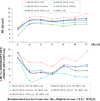 |
Fig. D.2 CO BEs for a growing ΔRLL and various low-levels of theory. See legend of Figure D.1 for further details. |
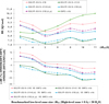 |
Fig. D.3 CH4 BEs for a growing ΔRLL and various low-levels of theory. See legend of Figure D.1 for further details. |
Regarding CO-related series in Fig. D.2, as for ONIOM(B3LYP-D3/6-311+G(d,p):GFN2-xtb), all series quickly converge with the low-level size, at ΔRLL of 4 Å, except for ONIOM(B3LYP-D3/6-311+G(d,p):B3LYP-D3/6-31G). In terms of the relative deviations with regard to a semiempirical xtb low-level treatment, these are globally below 15% at ΔRLL larger than 4 Å, except for ONIOM(B3LYP-D3/6-311+G(d,p):B3LYP-D3/6-31G). This indicates that the cheaper semiempirical GFN2-xtb method is well parameterized to describe such a dipole-dipole binding interaction.
Concerning finally the trends obtained for CH4 (Fig. D.3), xtb performances are weaker, but further validate the choice of a ΔRLL of 8 Å in order to make a good trade-off between the stability of the BE values with respect to the system size, as well as the reliability of the low-level method and its consistency with increasing low-level sizes. More specifically, the convergence of the BE series against growing low-level size appears at a ΔRLL larger than 6 to 8 Å for full ONIOM(DFT:DFT) frameworks, before the previously discussed convergence of the ONIOM(DFT:xtb) results. The trend followed by the latter series actually differs from those with systems treated at the ONIOM(DFT:DFT) level, while relative trends between ONIOM(DFT:DFT) series themselves are globally consistent. ΔBE between ONIOM(DFT:DFT) and ONIOM(DFT:xtb) frameworks increases at convergence of the ONIOM(DFT:DFT) series, from a ΔRLL larger than 6 to 8 Å. This was not observed for the CO and NH3 cases. This arguably points out a cooperative effect from the environment not well reproduced by GFN2-xtb. This can likely be attributed to the very weak interactions involved in the CH4 binding interactions, dominated by dispersion terms. In the case of NH3 and CO , stronger interactions were involved, imposing more constraints on the structure of the system. Their cooperative and extended long-range effects are better captured by the semiempirical xtb method. Quantitatively speaking, the relative differences with respect to a GFN2-xtb low-level treatment, at convergence of the BE series with growing ΔRLL in full DFT ONIOM schemes, amount to maximum ∼20% at ΔRLL of 8 Å, while it increases to ∼30% at worst at larger real system sizes compared to low-level treatment including diffuse functions.
We note also that the reliability of GFN2-xtb has already been widely validated for general purposes, as in the original Bannwarth et al. (2019) paper. In systems similar to our study, it has also been evaluated in Germain & Ugliengo (2020) and Tinacci et al. (2022). Our results are therefore complementary to their analysis, providing additional method-specific insights into the stability of xtb performance against growing ΔRLL.
Appendix E Automated script for an unbiased binding configurations sampling
An automated Python script has been written for the generation of all inputs needed for the unbiased sampling of the binding configurations of the three adsorbate test cases onto the modeled ASW surface, and the monitoring of each computations required to obtain the final BEs (geometry optimizations, frequency computations and BSSE evaluation). More specifically, the water box at the end of the last MD quenching phase is replicated in the x−y plane, taking advantage of the PBC. A grid of 10 by 10 equally spaced hemispheric centers is placed above the surface. The grid spacing is 4 Å, and avoids redundancy between adjacent adsorption sites. This has been validated through RMSD analysis as further discussed later one. These 100 points constitute the central points for the definition of each of the studied hemispheres based on distance discrimination (Rhem = 16 Å), taking advantage of the PBC in the x and y directions. The first starting guess of the adsorbate barycenter is then placed at 2 Åin z from each central point. This allows for the sampling of spatially distinct binding sites, and therefore accounts for the complexity of the surface typology. The adsorbate-to-substrate orientation is then defined for each grid point. The number of starting orientations depends on the adsorbate symmetry; for NH3, 3 starting orientations have been studied, with (i) with the three hydrogens toward the surface, (ii) with the 3 hydrogen flipped in the opposite direction in z , and (iii) with the plane passing by the three hydrogens being perpendicular to the surface. In the case of CO, 3 orientations have also been sampled, with (i) CO axis parallel to the surface, (ii) CO axis parallel to the normal to the surface, with O toward the surface, and (ii) CO axis parallel to the normal to the surface, with C pointing toward the surface. This defines the most representative/differing orientations, and seems to be the best compromise to sample as much as possible the different possible binding configurations while keeping a reasonable number of systems to be optimized and studied. On the other hand, regarding the symmetry of CH4, only one orientation has been studied for this adsorbate. This enables the sampling of the roughness of the local PES within each locally distinct binding site. The z-position of the adsorbate barycenter is then refined such that at least one adsorbate atom is at a distance lower than 3 Å from one water molecule from the substrate. Atoms are finally grouped by ONIOM-2 layers based on distance discrimination, avoiding any cut bonds at the boundaries, and input for geometry optimization at ONIOM(B3LYP-D3/6-311+G(d,p):GNF2-xtb) of theory are written. Tight convergence criteria5 are applied for the model zone, while default SCF parameters6 are used for GFN2-xtb low-level treatment. Each input is saved for each adsorbate, and subsequently submitted. The monitoring of each job is then ensured automatically through crontab scripts aimed at checking the status of each job (in run, finished normally due to reached convergence, or finished before convergence), and re-launch the appropriate computations until optimization, vibrational frequency (for zero-point energy correction) and BSSE correction computations are completed.
Appendix F RMSD analysis of binding configurations (including nearby water molecules)
As discussed in the main text, binding site redundancy reduction was applied before addressing the inferred BE distributions. More specifically, following our BE inference scheme, there are two potential source of redundancy (in terms of BE and RMSD of the surrounding nearest water molecules) in the binding behavior of a given adsorbate,
Redundancy between binding configurations on juxtaposed binding sites/hemispheric cuts. All in all, the inclusion or reduction of this first source of redundancy simply depends on the refinement of the sampling grid. For instance, in the method proposed by Tinacci et al. (2022), reduction was required. In our method, this has been avoided with a proper choice of our grid spacing for the binding site starting position sampling; that is, 4 (Å). We, however, still checked if no redundancy effectively stands out from the RMSD analysis of juxtaposed binding configurations, as justified in the following paragraphs.
Redundancy between binding configuration for different starting orientation of the adsorbate on a given hemispheric cut. This concerns the case of NH3 or CO ; if different starting orientations converge to the same local minimum, this has been reduced to the unique consideration of the distinct binding configuration per site. In the followings, this redundancy reduction is referred to as in-site binding configuration redundancy reduction.
In practice, in-site binding configuration redundancy analyses were performed under the following redundancy cutoffs: two binding configurations were considered to be redundant if ΔBEij < 0.05.<BE>ij kJ/mol7 and RMSD <1 Å, where <BE>ij is the mean BE for i and j orientations.
From these principles, starting from the working hypothesis that the sampled surface (40 × 40(Å)) combined to our grid density for the starting guess of adsorption site are statistically representative of a realistic interstellar cold environment ice, and knowing the total number of adsorption sites for a given typical grain surrounded by an icy mantle, the frequency count of each adsorption site can be directly retrieved.
For each system, the configuration considered for RMSD computation8 the adsorbate plus the x nearest9 water molecules from the adsorbate, x being equal to the mean number of nearby water molecules within an interaction zone defined by a radius of 3.2 Å from each adsorbate atom. Moreover, rotation was allowed in the RMSD minimization procedure. This allows one to have a constant number of coordinates to be compared through RMSD analysis, while avoiding as much as possible geometrical artifacts and properly quantify the surface structural diversity in terms of binding site.
Appendix F.1 NH3-related RMSD analyses
Fig. F.1 presents the full RMSD analysis for NH3 binding configuration sampling, in which each system associated with a valid BE (converged geometry optimization and validation after check of imaginary frequency) is compared to each other valid system. Systems are labeled between 0 and 300, one cut being associated with three successive numbers accounting for its three geometries.
From these results, several statistical tests have been performed. Foremost, Fig. F.2 gives the distributions of RMSD values and ΔBE for comparisons between optimized configurations of different NH3 starting orientations on the same cut. From these plots, it is clear that the different starting orientations have an impact on the final complex geometry. This enforces the requirement of sampling these different orientations within a given cut to enable an extensive sampling of the diversity of binding configuration, including the local roughness of the substrate potential energy landscape. Pairs of geometries with RMSD value below 1 Å and ΔBE are disregarded in the in-site binding configurations redundancy analysis procedure, as discussed in the main text. These cutoffs are justified by the present analysis; indeed, integrating the contributions between 0 and 1 Å and 0 and respectively for the RMSD and ΔBE histograms of Fig. F.2 yields consistent integrated densities, of 0.29% and 0.26%, respectively, supporting the coherence of the adopted thresholds.
 |
Fig. F.1 Full symmetric RMSD matrix results for the NH3 binding behavior study on ASW ice model – comparison only performed between systems leading to accepted BE values. |
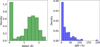 |
Fig. F.2 Histograms of (left) RMSD values, (right) ΔBE (%) for comparison of optimized configurations from the different NH3 starting orientations on the same cut. |
On the other hand, we also studied the RMSD value and corresponding ΔBE for the comparison of juxtaposed cuts, as shown in Fig. F.3. As we can see, the associated values are globally higher than 0.8 Å, and ΔBE (%) do not go below 5% (min. 6.4). Concerning the full distribution of RMSD value including all the computed value except diagonal terms (comparison of systems with themselves, strictly leading to zero RMSD value) is characterized by a mean value of 1.56 ± 0.39 Å. Excluding juxtaposed cuts as well as inter starting geometry intra cut contributions leads to a mean value of 1.56 ± 0.38 Å. These results confirm that the grid spacing has been well chosen and that the first potential source binding site sampling redundancy previously discussed has been effectively avoided.
Appendix F.2 CO-related RMSD analyses
Fig. F.4 presents the full RMSD analysis for the binding configuration sampling of CO.
These same statistical tests as applied to NH3 RMSD matrix have been applied, as shown in Figures F.5 and F.6 for the distributions of RMSD and ΔBE for the comparison respectively between optimized configurations of different CO starting orientations on the same cut, and between juxtaposed cuts.
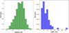 |
Fig. F.3 Histograms of (left) RMSD values, (right) ΔBE (%) for comparisons between optimized configurations of juxtaposed cuts, including all NH3 starting orientations. |
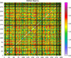 |
Fig. F.4 Full symmetric RMSD matrix results for the CO binding behavior study on ASW ice model – comparison only performed between systems leading to accepted BE values. |
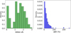 |
Fig. F.5 Histograms of (left) RMSD values, (right) ΔBE for comparisons between optimized configurations of different CO starting orientations on the same cut. |
These two analyses lead to very similar qualitative trends to the case of NH3. Once more, the coherence of the thresholds used for the definition of in-site redundancy is validated results in Fig.F.5, demonstrating the consistency of the integrated densities between 0 and 1 Å and 0 and respectively for the RMSD (0.20%) and ΔBE (0.18%) histograms. Concerning the full RMSD distribution except diagonal terms, one gets a mean value of 1.78 ± 0.50 Å. Excluding juxtaposed cuts as well as inter starting geometry intra cut contributions leads to a mean value of 1.79 ± 0.50 Å. These results therefore also validate that the different starting orientations of the adsorbate onto a same system impact the resulting complex adsorbate-substrate geometry, while our spacing for our sampling grid is adequately chosen to avoid a collapse into the same energy minimum and therefore a redundancy between adjacent binding sites.
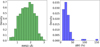 |
Fig. F.6 Histograms of (left) RMSD values, (right) ΔBE for comparisons between optimized configurations of juxtaposed cuts, including all CO starting orientations. |
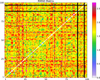 |
Fig. F.7 Full symmetric RMSD matrix results for the CH4 binding behavior study on ASW ice model – comparison only performed between systems leading to accepted BE values. |
Appendix F.3 CH4-related RMSD analyses
Remembering that the CH4 binding behavior has been studied from a single starting geometry per hemisphere due to its symmetry, the RMSD matrix is composed of a 100 × 100 grid, given in Fig. F.7.
The distributions of RMSD and ΔBE for the comparison between juxtaposed cuts is given in Figure F.8. Concerning the full RMSD distribution except diagonal terms, one gets a mean value of 1.79 ± 0.31 Å. Excluding juxtaposed cuts leads to a mean value of 1.78 ± 0.35 Å. As for the two previously discussed adsorbate, juxtaposed cut does not lead to small RMSD associated with negligible ΔBE values, meaning that the initial grid spacing effectively avoids redundancy between juxtaposed binding sites.
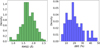 |
Fig. F.8 Histograms of (left) RMSD values, (right) ΔBE for comparisons between optimized configurations of juxtaposed cuts for CH4 as adsorbate. |
References
- Abascal, J. L. F., & Vega, C., 2005, J. Chem. Phys., 123, 234505 [Google Scholar]
- Bannwarth, C., Ehlert, S., & Grimme, S., 2019, J. Chem. Theory Comput., 15, 1652 [Google Scholar]
- Bannwarth, C., Caldeweyher, E., Ehlert, S., et al. 2021, WIRES Comput. Mol. Sci., 11, e1493 [Google Scholar]
- Beaujean, P., Champagne, B., Grimme, S., & de Wergifosse, M., 2021, J. Phys. Chem. Lett., 12, 9684 [Google Scholar]
- Boogert, A. C. A., Gerakines, P. A., & Whittet, D. C., 2015, ARA&A, 53, 541 [NASA ADS] [CrossRef] [Google Scholar]
- Bovolenta, G., Bovino, S., Vöhringer-Martinez, E., et al. 2020, Mol. Astrophys., 21, 11 [Google Scholar]
- Chung, L. W., Sameera, W. M. C., Ramozzi, R., et al. 2015, Chem. Rev., 115, 5678 [Google Scholar]
- Collings, M. P., Anderson, M. A., Chen, R., et al. 2004, MNRAS, 364, 1133 [Google Scholar]
- Crapsi, A., Caselli, P., Walmsley, M., & Tafalla, M., 2007, A&A, 470, 221 [NASA ADS] [CrossRef] [EDP Sciences] [Google Scholar]
- Dapprich, S., Komáromi, I., Bryun, K. S., Morokuma, K., & Frisch, M. J., 1999, J. Mol. Struct. THEOCHEM, 461, 1 [Google Scholar]
- Das, A., Sil, M., Gorai, P., Chakrabarti, S. K., & Loison, J.-C., 2018, ApJS, 237, 13 [NASA ADS] [CrossRef] [Google Scholar]
- Duflot, D., Toubin, C., & Monnerville, M., 2021, Front. Astron. Space Sci., 8, 16 [NASA ADS] [CrossRef] [Google Scholar]
- Dulieu, F., Amiaud, L., Congiu, E., et al. 2010, A&A, 512, 5 [Google Scholar]
- Ferrero, S., Zamirri, L., Ceccarelli, C., et al. 2020, ApJ, 904, 20 [Google Scholar]
- Finney, J. L., Hallbrucker, A., Kohl, I., Soper, A. K., & Bowron, D. T., 2002, Phys. Rev. Lett, 88, 225503 [Google Scholar]
- Frisch, M. J., Trucks, G. W., Schlegel, H. B., et al. 2016, Gaussian 16, Revision C.01 (Wallingford, CT: Gaussian, Inc.) [Google Scholar]
- Fuchs, G. W., Cuppen, H. M., Ioppolo, S., et al. 2009, A&A, 505, 629 [NASA ADS] [CrossRef] [EDP Sciences] [Google Scholar]
- Furuya, K., 2024, ApJ, 974, 115 [NASA ADS] [CrossRef] [Google Scholar]
- Ganeshan, S., Ramírez, R., & Fernández-Serra, M. V., 2013, Phys. Rev. B Condens. Matter, 87, 134207 [Google Scholar]
- Germain, A., & Ugliengo, P., 2020, in ICCSA, eds. O. Gervasi, et al. [Google Scholar]
- Gould, R. J., & Salpeter, E. E., 1963, ApJ, 138, 393 [NASA ADS] [CrossRef] [Google Scholar]
- Grassi, T., Bovino, S., Caselli, P., et al. 2020, A&A, 643, A115 [Google Scholar]
- Grimme, S., Antony, J., Ehrlich, S., & Krieg, H., 2010, J. Chem. Phys., 132, 154104 [Google Scholar]
- Grimme, S., Ehrlich, S., & Goerigk, L., 2011, J. Comput. Chem., 32, 1456 [Google Scholar]
- Hama, T., & Watanabe, N., 2013, Chem. Rev., 113, 8783 [Google Scholar]
- He, J., Acharyya, K., & Vidali, G., 2016, ApJ, 825, 10 [NASA ADS] [CrossRef] [Google Scholar]
- Hollenbach, D., & Salpeter, E. E., 1971, ApJ, 163, 155 [NASA ADS] [CrossRef] [Google Scholar]
- Humphrey, W., Dalke, A., & Schulten, K., 1996, J. Mol. Graph., 14, 33 [Google Scholar]
- Ioppolo, S., van Boheemen, Y., Cuppen, H. M., van Dishoeck, E. F., & Linnartz, H., 2011, MNRAS, 413, 2281 [NASA ADS] [CrossRef] [Google Scholar]
- Kamp, I., Thi, W.-F., Woitke, P., et al. 2017, A&A, 607, 23 [Google Scholar]
- Karadakov, P. B., & Morokuma, K., 2000, Chem. Phys. Lett., 317, 589 [Google Scholar]
- Karssemeijer, L. J., Ioppolo, S., van Hemert, M. C., et al. 2014, ApJ, 781, 16 [Google Scholar]
- Keto, E., & Caselli, P., 2010, MNRAS, 402, 1625 [Google Scholar]
- Kouchi, A., Tsuge, M., Hama, T., et al. 2021a, MNRAS, 505, 1530 [CrossRef] [Google Scholar]
- Kouchi, A., Tsuge, M., Hama, T., et al. 2021b, ApJ, 918, 20 [Google Scholar]
- Kraus, P., Obenchain, D. A., & Frank, I., 2018, J. Phys. Chem. A, 122, 1077 [Google Scholar]
- Lee, C., Yang, W., & Parr, R. G., 1988, Phys. Rev. B Condens. Matter, 37, 785 [Google Scholar]
- Mariedahl, D., Perakis, F., Späh, A., et al. 2018, J. Phys. Chem. B, 122, 7616 [Google Scholar]
- Martinez, L., Andrade, R., Birgin, E. G., & Martínez, J. M., 2009, J. Comput. Chem., 30, 2157 [CrossRef] [Google Scholar]
- McClure, M., Rocha, W. R. M., Pontoppidan, K. M., et al. 2023, Nat. Astron., 7, 431 [NASA ADS] [CrossRef] [Google Scholar]
- Michoulier, G., Noble, J. A., Simon, A., Mascetti, J., & Toubin, C., 2018, PCCP, 20, 8753 [Google Scholar]
- Minissale, M., Loison, J.-C., Baouche, S., et al. 2015, A&A, 577, A2 [NASA ADS] [CrossRef] [EDP Sciences] [Google Scholar]
- Minissale, M., Aikawa, Y., Bergin, E., et al. 2022, ACS Earth Space Chem., 6, 597 [NASA ADS] [CrossRef] [Google Scholar]
- Miyauchi, N., Hidaka, H., Chigai, T., et al. 2008, Chem. Phys. Lett., 456, 27 [CrossRef] [Google Scholar]
- Molpeceres, G., & Kästner, J., 2020, PCCP, 22, 7552 [NASA ADS] [CrossRef] [Google Scholar]
- Molpeceres, G., Rimola, A., Ceccarelli, C., et al. 2018, MNRAS, 482, 5389 [Google Scholar]
- Molpeceres, G., Zaverkin, V., & Kästner, J., 2020, MNRAS, 499, 1373 [Google Scholar]
- Narten, A. H., Venkatesh, C. G., & Rice, S. A., 1976, J. Chem. Phys., 64, 1106 [NASA ADS] [CrossRef] [Google Scholar]
- Noble, J. A., Theule, P., Mispelaer, F., et al. 2012, A&A, 543, A5 [NASA ADS] [CrossRef] [EDP Sciences] [Google Scholar]
- Oba, Y., Watanabe, N., Hama, T., et al. 2012, ApJ, 749, 67 [Google Scholar]
- Oberg, K., 2016, Chem. Rev., 116, 9631 [CrossRef] [Google Scholar]
- Öberg, K. I., Boogert, A. C. A., Pontoppidan, K. M., et al. 2011, ApJ, 740, 109 [Google Scholar]
- Pedregosa, F., Varoquaux, G., Gramfort, A., et al. 2011, JMLR, 12, 2825 [Google Scholar]
- Penteado, E. M., Walsh, C., & Cuppen, H. M., 2017, ApJ, 844, 13 [NASA ADS] [CrossRef] [Google Scholar]
- Phillips, J. C., Hardy, D. J., Maia, J. D. C., et al. 2020, J. Chem. Phys., 153, 044130 [Google Scholar]
- Pirim, C., & Krim, L., 2011, Chem. Phys., 380, 67 [Google Scholar]
- Shimonishi, T., Nakatani, N., Furuya, K., & Hama, T., 2018, ApJ, 855, 11 [NASA ADS] [CrossRef] [Google Scholar]
- Sipilä, O., Caselli, P., Redaelli, E., Juvela, M., & Bizzocchi, L., 2019, MNRAS, 487, 1269 [Google Scholar]
- Smith, R. G., Sellgren, K., & Tokunaga, A. T., 1989, ApJ, 344, 413 [CrossRef] [Google Scholar]
- Song, L., & Kästner, J., 2016, PCCP, 18, 29278 [Google Scholar]
- Song, L., & Kästner, J., 2017, ApJ, 850, 9 [Google Scholar]
- Sure, R., & Grimme, S., 2013, J. Comput. Chem., 34, 1672 [CrossRef] [Google Scholar]
- Svensson, M., Humbel, S., Froese, R. D. J., et al. 1996, J. Phys. Chem., 100, 19357 [Google Scholar]
- Tielens, A. G. G. M., & Hagen, W., 1982, A&A, 114, 245 [Google Scholar]
- Tinacci, L., Germain, A., Pantaleone, S., et al. 2022, ACS Earth Space Chem., 6, 1514 [NASA ADS] [CrossRef] [Google Scholar]
- Vreven, T., Bryun, K. S., Komáromi, I., et al. 2006, J. Chem. Theory Comput., 2, 815 [Google Scholar]
- Wakelam, V., Loison, J.-C., Mereau, R., & Ruaud, M., 2017, Mol. Astrophys., 6, 22 [NASA ADS] [CrossRef] [Google Scholar]
- Watson, W. D., & Salpeter, E. E., 1972, ApJ, 174, 321 [NASA ADS] [CrossRef] [Google Scholar]
The native implementation of B97 functional in Gaussian is defined along with the D2 dispersion from the Grimme’s group.
The optimized configuration is defined by both the final adsorbate-to-substrate orientation and the associated feedback onto the relative orientation of the surrounding water molecules after geometry optimization.
These are defined with the following cutoffs: Maximum force <1.5 × 10⁻⁴ Hartree/bohr, RMS force <1.0 × 10⁻⁴ Hartree/bohr, maximum displacement <6.0 × 10⁻⁴ bohr, and RMS displacement <4.0 × 10⁻⁴ bohr.
10−6 Hartree for the energy and 10−4 e for the wavefunction.
This scaling of the cutoff on the ΔBE with the mean BE of the compared configurations is more consistent than a fixed ΔBE cutoff (e.g. 1 kJ/mol). It actually ensures the same strictness of the criterion whatever the adsorbate and characteristic BEs.
Note that all RMSD analyses presented in this Appendix were performed using the open source RMSD computation project available at https://github.com/charnley/rmsd.
Nearest H2O are defined by ordering the minimum distance between each water molecule and adsorbate atoms. In other words, for each water molecule from the substrate, the distance between each of its constitutive atoms and the atoms from the adsorbate was computed, and the minimum distance was kept for the ordering process of nearby water molecules.
All Tables
DFT functional benchmark results with respect to CCSD(T) over the three adsorbate test cases.
All Figures
|
Fig. 1 Comparison between the structure modeled through MD simulation in this work (continuous line), and the experimental results from Mariedahl et al. (2018) (dashed line), with (a) RDF for the O-O distance and (b) running coordination number for ASW-LDA ices analogs. |
| In the text | |
|
Fig. 2 Normalized histogram of sampled NH3 BE (in kJ/mol), fitted with a GMM using scikit-learn algorithm (Pedregosa et al. 2011). Previously reported NH3 BE values onto water ice analogs with diverse simulation methods are given on top. Horizontal intervals report on published BE dispersions, while vertical dashed lines relate to works focusing on single BE values. Methods used in each work are discussed in the text. The BE value on crystalline ice from Ferrero et al. (2020) is also given (plain gray line). Ref: [1] Ferrero et al. (2020); [2] Duflot et al. (2021); [3] Tinacci et al. (2022); [4] UMIST , [5] Wakelam et al. (2017)/KIDA; [6] Das et al. (2018); [7] Penteado et al. (2017); [8] Ferrero et al. (2020) on crystalline ice. |
| In the text | |
|
Fig. 3 Normalized histogram of sampled BEs (in kJ/mol) for CO, fitted with a single component gaussian profile. Previously reported results of CO BE values onto water ice analogs with diverse simulation methods are given on top. See Fig. 2 for the meaning of horizontal intervals, vertical dashed lines, and the plain gray line. Ref: [1] Ferrero et al. (2020); [2] He et al. (2016) and Penteado et al. (2017); [3] UMIST; [4] Wakelam et al. (2017)/KIDA, [5] Das et al. (2018); [6] Ferrero et al. (2020) on crystalline ice. |
| In the text | |
|
Fig. 4 Normalized histogram of sampled BEs (in kJ/mol) for CH4, fitted with a single component Gaussian profile. Previously reported results of CH4 BE values onto water ice analogs are given on top. See Fig. 2 for the meaning of horizontal intervals, vertical dashed lines, and the plain gray line. Ref: [1] Ferrero et al. (2020); [2] Smith et al. (1989), He et al. (2016), and Penteado et al. (2017); [3] UMIST; [4] KIDA, [5] Wakelam et al. (2017); [6] Das et al. (2018); [7] Ferrero et al. (2020) on crystalline ice. |
| In the text | |
|
Fig. 5 Statistical analysis of subgroup contributions using stacked histograms normalized on the global BE distribution for NH3, each subgroups representing a type of adsorbate-ice H-bond configuration. |
| In the text | |
|
Fig. 6 Subgroup contributions of θ value ranges using stacked histograms normalized on the global BE distribution for CO. |
| In the text | |
|
Fig. 7 Linear correlation between the electronic BEs and the ZPE corrected values (best fit – dashed line) for NH3 (blue), CO (green) and CH4 (orange) on ASW ice. |
| In the text | |
|
Fig. 8 Bootstrapping analysis of GMM two components statistics of NH3 BE distribution, with increasing set size. The set size definition depends on the number of picked adsorbate orientation per cut, increasing from 1 to 3 from the left to the right. The dashed line represents the statistics for the full set of data, while the continuous lines encompass a tolerance interval of 5% around these statistics. |
| In the text | |
|
Fig. 9 Bootstrapping analysis of mean BE and standard deviation of CO on LDA ice, with increasing set size. The set size definition depends on the number of picked adsorbate orientation per cut, increasing from 1 to 3 from the left to the right. |
| In the text | |
|
Fig. 10 Bootstrapping analysis of mean BE and standard deviation of CH4 on LDA ice, with increasing set size. The set size is defined by the number of picked random hemispherical systems. |
| In the text | |
|
Fig. A.1 Intermolecular O–O, O–H and H–H RDFs from this work, Mariedahl et al. (2018) and Michoulier et al. (2018) (with Narten et al. 1976 and Finney et al. 2002 data used in Michoulier et al. 2018). |
| In the text | |
|
Fig. B.1 DFT-functional benchmark on the tetrameric structures; orange and blue series account respectively for results with 6-311+G(d,p) and aug-cc-pVTZ as basis set – left column: difference with respect to CCSD(T) value. CCSD(T) reference BE and BSSE correction values are given explicitly; right column: relative difference with respect to CCSD(T) value in%. Graphs are going by pairs (raw), with the first raw being attributed to NH3, the second to CO and the third to CH4. The last raw gives the MARDs over the three adsorbates. |
| In the text | |
|
Fig. C.1 (top panel) NH3 BEs on a first tested binding site for a growing ΔRLowLevel, going from 3 to 11 Å, for a total radius between 11 and 19 Å. 4 different basis set for the high-level treatment are tested, as given in the legend of the plot, within an ONIOM(B3LYP-D3(BJ)/basis set:xtb) framework; (middle panel) Relative BE difference with respect to BE at ΔRLowLevel equal to 11 Å, each series being treated independently; and (bottom panel) Relative BE discrepancies relative to BE at B3LYP-D3(BJ)/aug-cc-pVTZ high level of theory, with ΔRLowLevel equal to 11 Å. |
| In the text | |
|
Fig. C.2 CO BEs on a first tested binding site for a growing ΔRLowLevel, going from 3 to 11 Å, for a total radius between 11 and 19 Å. Four different basis set for the high-level treatment are tested, as given in the legend of the plot, within an ONIOM(B3LYP-D3(BJ)/basis set:xtb) framework. See legend Fig. C.1 for the description of each panel. |
| In the text | |
|
Fig. C.3 CH4 BEs on a first tested binding site for a growing ΔRLowLevel, going from 3 to 11 Å, for a total radius between 11 and 19 Å. Four different basis set for the high-level treatment are tested, as given in the legend of the plot, within an ONIOM(B3LYP-D3(BJ)/basis set:xtb) framework. See legend Fig. C.1 for the description of each panel. |
| In the text | |
|
Fig. C.4 NH3 BEs on a second tested binding site for a growing ΔRLowLevel, going from 3 to 11 Å, for a total radius between 11 and 19 Å. Four different basis set for the high-level treatment are tested, as given in the legend of the plot, within an ONIOM(B3LYP-D3(BJ)/basis set:xtb) framework. See legend Fig. C.1 for the description of each panel. |
| In the text | |
|
Fig. D.1 Top panel – NH3 BE for a growing ΔRLL and various low-levels of theory. The different series hold for a computational scheme following ONIOM(B3LYP-D3/6-311+G(d,p): x), where x , the low-level method, accounts for either for B3LYP-D3/growing basis set (see legend), or GFN2-xtb; Bottom panel – residue graph representing the relative difference between ONIOM(B3LYP-D3/6-311+G(d,p):GFN2-xtb) and ONIOM(B3LYP-D3/6-311+G(d,p): B3LYP-D3/growing basis set). Note that legends only explicit the low-level method of each series, for the sake of clarity. Lines do not represent any interpolated physical trends, they only serve as guides to highlight the trend and facilitate the reader view of the plots. |
| In the text | |
|
Fig. D.2 CO BEs for a growing ΔRLL and various low-levels of theory. See legend of Figure D.1 for further details. |
| In the text | |
|
Fig. D.3 CH4 BEs for a growing ΔRLL and various low-levels of theory. See legend of Figure D.1 for further details. |
| In the text | |
|
Fig. F.1 Full symmetric RMSD matrix results for the NH3 binding behavior study on ASW ice model – comparison only performed between systems leading to accepted BE values. |
| In the text | |
|
Fig. F.2 Histograms of (left) RMSD values, (right) ΔBE (%) for comparison of optimized configurations from the different NH3 starting orientations on the same cut. |
| In the text | |
|
Fig. F.3 Histograms of (left) RMSD values, (right) ΔBE (%) for comparisons between optimized configurations of juxtaposed cuts, including all NH3 starting orientations. |
| In the text | |
|
Fig. F.4 Full symmetric RMSD matrix results for the CO binding behavior study on ASW ice model – comparison only performed between systems leading to accepted BE values. |
| In the text | |
|
Fig. F.5 Histograms of (left) RMSD values, (right) ΔBE for comparisons between optimized configurations of different CO starting orientations on the same cut. |
| In the text | |
|
Fig. F.6 Histograms of (left) RMSD values, (right) ΔBE for comparisons between optimized configurations of juxtaposed cuts, including all CO starting orientations. |
| In the text | |
|
Fig. F.7 Full symmetric RMSD matrix results for the CH4 binding behavior study on ASW ice model – comparison only performed between systems leading to accepted BE values. |
| In the text | |
|
Fig. F.8 Histograms of (left) RMSD values, (right) ΔBE for comparisons between optimized configurations of juxtaposed cuts for CH4 as adsorbate. |
| In the text | |
Current usage metrics show cumulative count of Article Views (full-text article views including HTML views, PDF and ePub downloads, according to the available data) and Abstracts Views on Vision4Press platform.
Data correspond to usage on the plateform after 2015. The current usage metrics is available 48-96 hours after online publication and is updated daily on week days.
Initial download of the metrics may take a while.