| Issue |
A&A
Volume 696, April 2025
|
|
|---|---|---|
| Article Number | A71 | |
| Number of page(s) | 8 | |
| Section | Interstellar and circumstellar matter | |
| DOI | https://doi.org/10.1051/0004-6361/202451665 | |
| Published online | 04 April 2025 | |
Role of NH3 binding energy in the early evolution of protostellar cores
1
Centre for Astrochemical Studies, Max Planck Institute for Extraterrestrial Physics,
Giessenbachstraße 1,
85748
Garching, Germany
2
Laboratoire d’Instrumentation et de Recherche en Astrophysique, CY Cergy Paris Université, Observatoire de Paris, PSL University, Sorbonne Université, Université Paris Cité, CNRS,
95000
Cergy,
France
★ Corresponding author; shreyaks@mpe.mpg.de
Received:
26
July
2024
Accepted:
17
February
2025
Context. NH3 (ammonia) plays a critical role in the chemistry of star and planet formation, yet uncertainties in its binding energy (BE) values complicate accurate estimates of its abundance. Recent research suggests a multi-binding energy approach, challenging the previous single-value notion.
Aims. In this work, we use different values of NH3 binding energy to examine its effects on the NH3 abundances and the chemistry of Class 0 protostellar cores.
Methods. Using a gas-grain chemical network, we systematically vary the values of NH3 binding energies in a model of a Class 0 protostellar core (using the model of IRAS 16293-2422 as a template) and study the effects of these binding energies on the NH3 abundances.
Results. Simulations indicate that, in our model, the abundance profiles of NH3 are highly sensitive to the binding energy used, particularly in the warmer inner regions of the core. Higher binding energies lead to lower gas-phase NH3 abundances, while lower values of binding energy have the opposite effect. Furthermore, this BE-dependent abundance variation of NH3 significantly affects the formation pathways and abundances of key species such as HNC, HCN, and CN. Our tests also reveal that the size variation of the emitting region due to binding energy becomes discernible only with beam sizes of 10 arcsec or less.
Conclusions. These findings underscore the importance of considering a range of binding energies in astrochemical models and highlight the need for higher resolution observations to better understand the subtleties of molecular cloud chemistry and star formation processes.
Key words: astrochemistry / radiative transfer / stars: protostars / ISM: abundances / ISM: molecules
© The Authors 2025
 Open Access article, published by EDP Sciences, under the terms of the Creative Commons Attribution License (https://creativecommons.org/licenses/by/4.0), which permits unrestricted use, distribution, and reproduction in any medium, provided the original work is properly cited.
This article is published in open access under the Subscribe to Open model.
Open Access funding provided by Max Planck Society.
1 Introduction
Since its detection (Cheung et al. 1968), NH3 has been ubiquitously observed in a variety of environments such as molecular clouds (Irvine et al. 1987), prestellar cores (Crapsi et al. 2007), the galactic centre (Winnewisser et al. 1979), diffuse clouds (Liszt et al. 2006), galaxies (Sandqvist et al. 2017; Gorski et al. 2018), star-forming regions (Fehér et al. 2022), comets (Poch et al. 2020), and planet-forming disks (Salinas et al. 2016). It is one of the six major molecules found in interstellar ices in the solid form (Boogert et al. 2015). It serves as an important tracer in the interiors of dense, starless cores where common tracers such as CO and CS are depleted from the gas phase onto dust grains (Caselli et al. 1999; Tafalla et al. 2002) due to temperatures as low as ~6K (Crapsi et al. 2007; Pagani et al. 2007) and number densities between 104 and 106 cm−3 (Keto & Caselli 2010). Although NH3 is affected by freeze-out (Caselli et al. 2022; Pineda et al. 2022; Lin et al. 2023), NH3 is selectively tracing dense material (Johnstone et al. 2010), as it is not abundant in the molecular cloud surrounding dense cores (unlike CO and CS).
An important parameter that influences the grain surface abundance of NH3 (and other species) is the binding energy. It serves as a measure of the strength of the interaction between the species and an adsorbate or grain surface. Additionally, once the species is adsorbed onto dust grains, the binding energy plays a crucial role in governing both its diffusion across and residence time on the grain surface. These factors, in turn, significantly influence the physical and chemical conditions governing the evolution of star-forming regions. For example, in the vicinity of a low-mass protostar, the binding energy determines the distance from the central protostar at which sublimation fronts emerge due to the desorption of volatile species from ice grain surfaces. Furthermore, the location of these sublimation fronts, also known as “snowlines” in protoplanetary disks, directly shapes the composition of the planets forming within protoplanetary disks. Hence, precise knowledge of the binding energies is critical for an accurate interpretation of observational data and reliable prediction of abundances through simulations.
Earlier studies, such as Hama & Watanabe (2013), Penteado et al. (2017), and Wakelam et al. (2017), provided a singular binding energy value for NH3 on different types of water ice. However, recent research has challenged this notion, suggesting that NH3 exhibits a distribution of binding energies. Experiments conducted by He et al. (2016) reveal a coverage-dependent distribution of binding energies for NH3 at sub-monolayer coverages. Additionally, Kakkenpara Suresh et al. (2024) observe a distribution of binding energies on crystalline ice (3780–4080 K) and compact amorphous solid water ice (3630–5280 K) at monolayer coverages. Theoretical calculations by Ferrero et al. (2020), Tinacci et al. (2022), and Germain et al. (2022) have further reinforce this conclusion, taking into account factors such as the presence of dangling oxygen (dO) and dangling hydrogen bonds, the orientation of the incoming molecule relative to the grain surface, and the structural properties of the grain. The notion of a binding energy distribution is logical given that the structure of ice on dust grains is amorphous, resulting in the formation of diverse and unique adsorption sites. This idea is further substantiated by Bovolenta et al. (2020), who obtain a Gaussianlike distribution of binding energies for hydrogen fluoride on amorphous solid water (ASW).
In their numerical study, Grassi et al. (2020) illustrate that employing a binding energy distribution allows molecules to occupy higher energy binding sites, thereby increasing their residence time on the grain surface. This prolonged residence time enhances their availability to react with other molecules, even at dust temperatures that conventionally exhibit limited or no reactivity. Building upon their findings and our previous work in Kakkenpara Suresh et al. (2024), the present study evaluates the influence of incorporating a range of binding energy values for NH3 in astrochemical models, in particular the impact of binding energy on the abundance distribution of NH3. We also investigate the possible effect that NH3 abundance variations may have on the distributions of other molecules chemically linked to NH3. Through a series of simulations, we have confirmed that the measured binding energies do not significantly influence the chemistry in prestellar cores. Hence, in the present work, we focus our attention on protostellar cores. We focus on the very early stages of the evolution of a protostellar core, and use a model of the well-studied class 0 protostellar core, IRAS 16293-2422, as a template for our simulations.
This work is organised in the following way. In Section 2, we outline the physical and chemical model of the protostellar core used. Section 3 presents our results, and Section 4 delves into the implications of these findings along with potential avenues for future research. A concise summary of our work is provided in Section 5.
2 Model
2.1 Physical model
The core is characterized using the model by Crimier et al. (2010) (Fig. 1), where the radial density profile follows as n(H2) ∝ r−1.8 within 6900 AU from the centre, and n(H2) is the H2 number density. In the study by Crimier et al. (2010), the density and dust temperature for the protostellar source IRAS 16293-2422 are derived from single-dish and interferometric continuum data spanning from millimeter to mid-infrared wavelengths. The study identifies a warm, inner component, modelled as a single source, despite interferometric observations revealing IRAS 16293-2422 to be a multi-source system (Maureira et al. 2020). In the present work, we treat the object as a single source, consistent with the single-dish data, as our objective is to use the Crimier et al. (2010) model as a representative template for a protostellar core rather than to replicate the specific observations of IRAS 16293-2422. The source exhibits a pronounced temperature and density gradient. In this model, the temperature of the gas rises significantly towards the interior due to both gas compression during collapse and radiation emitted by the protostar. We assume that the dust temperature and the gas kinetic temperature are equivalent. The analytical approach involved dividing the core into concentric shells, and the final results are combined radially. A two-phase (gas + ice) chemical model with a dust grain radius = 0.1 μm is employed, where the entire ice layer covering the grain is available for desorption.
The abundance profiles are obtained in two steps. First, the initial conditions corresponding to the parent cloud are obtained by running a single-point simulation with Tdust = Tgas = 10 K, n(H2) = 104 cm−3, grain radius = 0.1 μm, cosmicray ionisation rate, ζ = 1.3×10⁻¹⁷ s−1, and visual extinction AV = 10 mag. Adsorption and desorption, including mechanisms such as photodesorption, thermal and chemical desorption, and cosmic ray-induced desorption, are considered in the model. Reactive desorption is treated following Garrod et al. (2007), assuming a typical efficiency of 1% regardless of the desorbing species. Mechanisms such as the Eley-Rideal mechanism and non-diffusive chemistry are not included in the present model. The rates of photoprocesses are calculated as a function of AV, following the parameterisation provided on the KInetic Database for Astrochemistry (KIDA)1 webpage. These rates are calculated based on the expression for the ‘standard’ interstellar radiation field (ISRF) from Draine (1978), as specified on the KIDA webpage. The simulation is allowed to proceed until a time, t1 = 106 years, consistent with the previous work of Brünken et al. (2014) and Harju et al. (2017) on the source. At this stage, the abundances of all the species are extracted. These are then used as the initial abundances to trace the evolution of the protostellar core.
The grain radius and the cosmic-ray ionisation rate, ζ, are not changed in this step; however, the visual extinction AV ranges from 2000 mag in the inner regions to 10 mag at the core edge. Finally, the abundances are extracted after an evolutionary time of t2 = 104 years. Numerical studies (Boss & Yorke 1995; Hincelin et al. 2016; Navarro-Almaida et al. 2024) suggest that this time corresponds to the formation of the First Larson Core (or the First Hydrostatic Core). Our choice of t2 ensures that the simulation captures an early evolutionary stage before the development of substructures, such as disks, which are expected to form within the inner regions on timescales of 104–105 years (Gerin et al. 2015). Since the present static physical model does not account for such substructures, selecting an early time allows sufficient time for chemical evolution while providing an estimate of the initial chemical conditions of the forming small-scale structures.
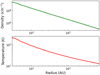 |
Fig. 1 Top: The H2 number density and bottom: the temperature distribution assumed to model IRAS 16293-2422. |
Initial chemical abundances with respect to total H nuclei, nH.
2.2 Chemical model
The chemical evolution of the core is monitored by the gas-grain chemical code, pyRate, discussed in Sipilä (2012); Sipilä et al. (2010). The model is pseudo-time dependent, that is, we track the chemical evolution assuming a static core. pyRate employs the rate equation method for computing the molecular abundances. The gas-phase network is constructed based on the kida.uva.2014 network (Wakelam et al. 2015), with modifications to incorporate deuterated species and spin state chemistry (Sipilä et al. 2015a,b). Here, we employed a large chemical network that contains a combined total of over 75 000 reactions in the gas phase and on grain surfaces, with which we simulated the chemistry of NH3 and its deuterated forms. In addition, the KIDA network is also used to study the effect of proton transfer reactions on the abundances of NH3 (Section 4.2).
Initially, the species are assumed to be atomic, except for H2 and HD, and the initial ortho/para H2 ratio is set to 10−3, consistent with a spin temperature, Tspin ~ 20 K (Brünken et al. 2014; Crabtree et al. 2011). Choosing this specific value for the ratio of ortho/para H2 corresponds to the assumption that the spin-state ratio has had the time to undergo thermalisation prior to the formation of the core. The initial abundances of the species are provided in Table 1. The binding energies for NH3 on water ice surfaces are sourced from Kakkenpara Suresh et al. (2024). Binding energies of various other species on water ice are obtained from Garrod & Herbst (2006) and Sipilä (2012). Although the model tracks the ortho and para forms of NH3 separately, the simulated abundances presented here represent their combined total.
3 Results
3.1 Abundance profiles
Motivated by the experimental results of Kakkenpara Suresh et al. (2024), we investigated how variations in NH3 binding energy impact the chemical composition of a protostellar core. For this purpose, we conducted a series of simulations where we systematically varied only the binding energy of NH3 in each model and traced the resulting chemical evolution with time within the core.
Figure 2 presents the abundances of NH3 in the gas-phase and on grain surfaces with respect to the radial distance from the centre to the outer edges of the core. The gas-phase abundance of NH3 decreases moving radially inwards toward the centre of the core, before increasing rapidly by several orders of magnitude. The abundance profile shows clear differentiation based on the value of binding energy employed. The region of high NH3 gas-phase abundance appears closer to the centre, with the radius of the desorption zone varying between 150 and 300 AU with increasing binding energy value used. Investigation of the reaction rates at this time step revealed that the primary contributor influencing NH3 gas-phase abundances is thermal desorption from dust grains. As the binding energy increases, NH3 remains on the grains until a higher temperature is reached, at which point it acquires sufficient thermal energy for desorption. Varying the binding energy does not create or destroy ammonia; rather, it only shifts the effective temperature at which ammonia is thermally desorbed. The final amount of ammonia corresponds to the total abundance of thermally desorbed ammonia ice.
Notable related effects are seen in species such as HNC, CN, and HCN (Fig. 3). We find that their abundance profiles vary within the same spatial zone where NH3 abundances vary. The effects are directly tied via chemical reactions to the variations in the NH3 abundances. This effect is further discussed in Section 4.1. Furthermore, we analysed the relative abundances of key volatile compounds found in ices, namely NH3, CO, CO2, CH4, and CH3OH, with respect to H2O. We compared our predictions with the reported values in Boogert et al. (2015), but direct comparisons are challenging due to differences in the sources and uncertainties related to the parameters employed for calculating ice abundances in the cited study. Further details of these comparisons are available in Appendix A.
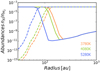 |
Fig. 2 Radial abundances of NH3 in gas phase (solid lines) and on grain surfaces (dashed lines) at 104 years. The binding energies of NH3 used in each model (colours) are displayed in the lower right corner. |
3.2 Column density maps of P-NH3
To assess the potential observational impact of the NH3 abundance variations, we simulated NH3 column density maps individually for each BE value. Here, we considered p-NH3 only so that we can compare the column density maps against the simulated emission of the (1,1) transition of this molecule (see Sect. 3.3). To generate the column density maps, we employed the radial abundances of p-NH3 obtained in the previous section as input, which are then interpolated to create a two-dimensional map of the cloud core. The abundances are convolved to a beam size of 2″ for the object situated at 120 pc to simulate interferometric observations (the distance to IRAS 16293-2422, although this can be applied to other similar sources by simply changing the distance value). The radial distribution of column density, denoted as N, is calculated using the formula:

Here, Σ represents the summation across i elements of the core model, p is the path length through an element i in cm, Xi is the abundance of the species (here, p-NH3) in i with respect to H2, and n(H2) is the volume density of i in mol cm−3. Figure 4 shows the 2D maps of column densities of p-NH3 within a 300 AU radius where the binding energy-dependent variations are apparent. The radius of the desorption zone decreases as the binding energy increases. The column density, as displayed in Fig. 4, traces the part of the distribution that could only be observed with specific NH3 lines, for example, the (1,1) inversion line. The column density maps also indicate the extent of desorbed NH3 that will be available in the gas phase.
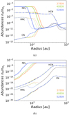 |
Fig. 3 Variation in the (a) gas-phase and (b) grain abundances of NH3, HNC, HCN and CN with binding energy. The colour scheme for the lines follows the same as in Fig. 2. |
3.3 Radiative transfer studies of the NH3 (1,1) transition
One-dimensional radiative transfer (RT) modelling of the 23 GHz (1,1) rotational-inversion transition of p-NH3 is carried out to verify the observability of the binding energy-dependent variation in the radius of the desorption zone. The non-local thermal equilibrium (LTE) radiative transfer code LOC (Juvela 2020) is used, which traces a predetermined set of rays through the model volume. The first step in this analysis is to simulate the cloud that contains the protostellar core and its envelope. Given that our template source is a Class 0 object that is embedded in a larger-scale cloud, for the purposes of the RT simulations, we have added an envelope outside the core. The methodology employed to determine NH3 abundances within the envelope closely follows the two-step approach outlined for the core in Section 2.1. First, we obtained the abundances corresponding to the parent cloud by running a single-point simulation for t1 = 106 years under the same conditions as the parent cloud, similar to that described in Section 2.1. After extracting the NH3 abundances at this stage, we ran a second single-point simulation, for t2 = 104 years, this time using the specific physical conditions for the envelope. These conditions include an envelope thickness set to 0.1 pc (5 × 1017 cm) assuming a visual extinction, AV = 5 mag, n(H2) = 104 m−3 and T = 10 K. The modelling is done taking into consideration the 18 hyperfine components of p-NH3. The velocity resolution is set to ~0.835 km/s such that it is high enough to distinguish the hyperfine components. The spectra are obtained for 1000 lines of sight across the radius of the whole object. Each spectrum is then convolved to a synthesized beam of 2″. The intensity of the transition from these spectra is integrated and interpolated to create a two-dimensional intensity map (Fig. 5), assuming spherical symmetry. The velocity field is computed based on a free-fall velocity profile, assuming a 2 M⊙ source at the centre, as detailed in Crimier et al. (2010) and Giers et al. (2023).
The collisional and radiative rate coefficients for the p-NH3 line simulations are taken from the LAMDA database (Schöier et al. 2005). The provided coefficients (collisional data from Danby et al. 1988) do not resolve the hyperfine structure, and hence we assumed that the coefficients for the individual hyperfine components were distributed according to LTE. To investigate the potential effect of hyperfine-resolved collisional rate coefficients on our results, we ran another series of line simulations adopting instead the set of collisional rate coefficients presented recently by Loreau et al. (2023). The hyperfine-resolved radiative transition frequencies and Einstein A coefficients were derived from data in the CDMS (Endres et al. 2016). These two approaches led only to small differences in simulated lines, and in what follows we present the results of simulations carried out using the data originating in LAMDA.
In each model, we observe that the peak intensity is centrally concentrated and declines going outwards. The location and size of this zone are in good agreement with the simulations of the column densities (Fig. 4), despite optical thickness effects that are missed by calculating the column density directly from the simulated abundances. Predominantly, the intensity originates from the inner zone due to elevated NH3 gas-phase abundance, as indicated by the abundance profiles (Fig. 2). Moreover, the size of the emitting region diminishes with higher binding energy, attributed to a reduction in gas-phase NH3 concentrations associated with increasing binding energy. Similar results are obtained for radiative transfer models using the (2,2) and (3,3) lines.
Convolutions of the spectra for the (1,1) transition at larger beam sizes are also conducted to evaluate the observability of this variation in the size of the emitting region. However, these effects become discernible only with beam sizes of 10 arcsec or smaller. This highlights the need for higher-resolution observations to detect such subtleties in the star-formation process. When convolved with a 6 arcsec beam, similar to the observations by Mundy et al. (1990), we obtain brightness temperatures lower than but within a factor of two compared to their reported value of 16.5 K for the NH3 (1,1) emission towards the brightest regions of their source – IRAS 16293-2422. They report NH3 emissions arising from a ring-like region of 3000–4000 AU with a resolution of 6 arcsec (960 AU). In contrast, the BE-related effects in the model used in the present work originate from a region smaller than 300 AU, indicating that higher resolution observations will be necessary to draw important conclusions regarding effects due to NH3 binding energy towards this source. Additionally, we ran radiative transfer models assuming higher velocity resolution (0.15 km/s) for the lines based on observations by Crapsi et al. (2007) using the Very Large Array (VLA), and found no difference in our results. Using the higher resolution requires more computational time, but does not impact the results, so we decided to retain the lower velocity resolution for our models.
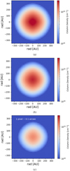 |
Fig. 4 Column density map of p-NH3 without the envelope (see text) for binding energy (a) 3870 K (b) 4080 K and (c) 5280 K. The angular size simulated by each pixel for each map is given in the top left corner of Fig. 4c. |
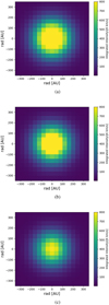 |
Fig. 5 Integrated intensity map of p-NH3 (1,1) in the core for binding energy (a) 3870 K (b) 4080 K and (c) 5280 K with envelope. |
4 Discussion
4.1 Influence of NH3 binding energy on abundance profiles of chemically related species
Interestingly, notable effects are observed on other species, and their abundance profiles within the same zone where NH3 abundances vary. A few examples are demonstrated in Fig. 3. The abundance profiles of these species vary depending on the chosen binding energy of NH3. To understand this, let us consider the example of HNC (Fig. 6). In the inner regions of the model with binding energy = 3780K, HNC is efficiently produced through the reaction between HCNH+ and NH3, yielding HCN and HNC. HCNH+ originates from HCN through the interaction with  and can revert to HCN via reactions between HCNH+ and H2CO (and HCNH+ + NH3). Hence, the connection between HCN and HNC follows the sequence HCN → HCNH+ → HNC, where the first step involves
  , and the second step involves NH3.
In contrast, in the model with binding energy = 5280 K, the gas phase abundance of NH3 is low, which effectively closes off the HCNH+ + NH3 route. HNC is being created instead via H-abstraction from H2CN (dashed arrow in Fig. 6), but at approximately ~10% of the rate of the NH3 route of the previous model; HNC formation is severely inhibited by the lack of available NH3. This can be seen in Fig. 3, where the shape of the HNC abundance profile follows that of NH3. Simultaneously, the rate of the reaction HCNH+ + H2CO → HCN + H2COH+ increases (as the HCNH+ destruction channel with NH3 is absent).
Studies by Jin et al. (2015) and Hacar et al. (2020) show that the HCN/HNC ratio, an important chemical thermometer, is sensitive to gas kinetic temperature, with HNC converting to HCN at higher temperatures – a trend also observed in our work. Therefore, it is plausible that variations in ammonia abundance, related to binding energy differences, influence the HCN/HNC ratio. This hypothesis warrants further investigation, which we plan to address in a future work. While HNC serves as an example of species influenced by variations in NH3 abundance due to changing binding energies, a detailed analysis of each species is necessary to determine the specific causes of these abundance differences, as they may not always result from direct reactions with NH3. Nevertheless, our findings underscore the importance of exploring the role of NH3 binding energy in determining the abundances of various species within protostellar cores.
4.2 Effect of proton transfer reactions on NH3 abundances
Taquet et al. (2016) demonstrate that methanol abundances are significantly enhanced through proton transfer reactions involving NH3, as compared to simulations lacking NH3. Subsequently, we introduced the following reaction
 (1)
(1)
which contributes to the synthesis of dimethyl ether or methyl formate. We then ran a new chemical simulation with this reaction included, wherein only NH3 binding energies were varied, to investigate potential effects on methanol abundances. For this test, we used the KIDA network (Wakelam et al. 2015) in place of our full deuterium and spin-state containing networks, for two main reasons: 1) to check if our overall conclusions on the binding energy-dependent NH3 desorption region remain unaffected regardless of the chemical network used (i.e. that the presence of deuterium and spin states does not affect the conclusions to a significant degree); and 2) to search for potential effects on some complex organic molecules (COMs) that are not included in our fiducial chemical network (for example, CH3OCH3, CH3CH2OH, etc). The grain-surface network used in this test is the same as our fiducial one, but with deuterium and spin states removed.
In the investigation of Taquet et al. (2016), protonation by NH3 extends the lifetime of methanol from 104 years to 105 years. In our study, methanol remains for up to 106 years even without their reaction integrated into the KIDA network. Upon inclusion of their reaction, our simulations validate their results, showing an increase in methanol abundances of up to two orders of magnitude for a specific binding energy value. However, we stress that this enhancement became noticeable only beyond 106 years. Analysis of abundances for different binding energy values at a specific time step reveals marginal variations in methanol abundances, even at 106 years, where the most substantial difference emerges between simulations with and without the proton-transfer reaction. The discrepancy in the evolutionary time in our model versus that of Taquet et al. (2016), regarding when the effect on CH3OH becomes apparent, is very likely due to different simulation parameters. We have not attempted to duplicate their results. Nevertheless, the comparison indicates that proton-transfer reactions can be very important and should be explored in more detail in later simulations.
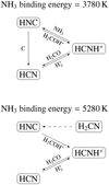 |
Fig. 6 Main formation and destruction pathways of HNC as predicted by the chemical model for the two extreme binding energy (BE) values. In the lower figure (BE = 5280 K), the dashed arrow represents an alternative pathway for the formation of HNC through H-abstraction from H2CN. This pathway becomes prominent when the gas-phase abundance of NH3 is low, thereby inhibiting the formation via the reaction between NH3 and HCNH+. |
5 Conclusions
NH3 is an important molecule, widely observed in various astronomical sources and on dust grain surfaces. However, uncertainties pertaining to its binding energy values prevent an accurate determination of its abundance and its role in the chemistry of star and planet formation. The binding energy is a key parameter determining the abundance and chemistry of a species in the ISM. Recent studies challenge previous notions of a unique binding energy value for NH3, proposing instead a multi-binding energy approach.
Drawing on previously established experimental work by Kakkenpara Suresh et al. (2024), we incorporated multiple NH3 binding energy values, derived from these studies, into gas-grain chemical simulations to examine their impact on NH3 abundance within a protostellar core. We conducted multiple simulations, systematically varying only the NH3 binding energy to discern its influence on the abundance profiles of NH3 and other species. Our findings reveal a distinct dependence of NH3 abundance profiles on the binding energy employed, particularly in the inner warm regions of the model. This variability extends its influence on other key species, including HCN, HNC, and CN, where the NH3 abundance dictates the preferred pathway for their formation. On the contrary, in proton transfer reactions involving NH3 , expected to enhance methanol formation, the abundance variation of NH3 due to binding energy does not appear to be a significant contributing factor.
Simulation of column density maps for p-NH3 reveals that the size of the desorption region diminishes as the binding energy increases. These findings align with radiative transfer studies on the (1,1) inversion line of NH3, where we added an envelope to our physical model to examine absorption and emission effects. In these studies, we observe that the peak intensity is centrally concentrated and decreases outward. Additionally, the intensity diminishes with higher binding energy, due to a reduction in gas-phase NH3. Our results highlight the importance of considering diverse binding energies in astrochemical models, providing a refined understanding of molecular cloud chemistry, and star formation processes.
For future work, it is crucial to refine our understanding by further exploring the impact of varied binding energies on complex organic molecules (COMs) within astrochemical models. Additionally, investigations into the spatial distribution and temporal evolution of species influenced by multi-binding energy approaches would contribute valuable insights. The present results apply at very early times in the core evolution, when the substructure is still absent, and, hence, probe the very early stages of forming protostellar systems. While the present work primarily focuses on the impact of different binding energies on the chemistry of protostellar cores, it is essential to refine their physical models by incorporating more accurate representations of the observed substructures within these sources. Such improvements are crucial for achieving a more precise and detailed understanding of the underlying phenomena in these sources.
Acknowledgements
The authors acknowledge the financial support of the Max Planck Society, CY Initiative of Excellence (grant “Investissements d’Avenir” ANR-16-IDEX-0008), the Programme National “Physique et Chimie du Milieu Interstellaire” (PCMI) of CNRS/INSU with INC/INP co-funded by CEA and CNES, a funding programme of the Region Ile de France.
Appendix A Relative Ice Abundances of Key Volatiles
In our model, low ice abundances in the central regions of the source, attributed to the high temperatures (approximately 200K), render these ice abundance values less meaningful. As a result, in Fig. A.1, we present simulated abundance ratios beyond 2000 AU only, where ice abundances are higher due to temperatures dropping to around 10–20 K. Our findings for CO and CH3OH align well with the range observed in low-mass young stellar objects (LYSOs) as described in Boogert et al. (2015). Although our estimates for CH4 abundances are slightly elevated, they remain reasonably close to the values reported in the Boogert et al. (2015). In our model, CO2 exhibits levels lower by two orders of magnitude, while NH3 is overestimated by a factor of three. These discrepancies may stem from a variety of factors, such as the elemental abundances used in our model, the impact of background emissions on the observed line intensities, or missing grain-surface chemistry (in the case of CO2). A comprehensive discussion of the cause of these variations exceeds the scope of our current study and is therefore omitted.
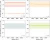 |
Fig. A.1 Relative ice abundances of key volatiles with respect to water ice. The solid lines represent values obtained in this work and the shaded zones of the same colour represent the range of observed values reported in Boogert et al. (2015) |
References
- Boogert, A. A., Gerakines, P. A., & Whittet, D. C. 2015, Annu. Rev. Astron. Astrophys., 53, 541 [CrossRef] [Google Scholar]
- Boss, A. P., & Yorke, H. W. 1995, ApJ, 439, L55 [NASA ADS] [CrossRef] [Google Scholar]
- Bovolenta, G., Bovino, S., Vöhringer-Martinez, E., et al. 2020, Mol. Astrophys., 21, 100095 [NASA ADS] [CrossRef] [Google Scholar]
- Brünken, S., Sipilä, O., Chambers, E. T., et al. 2014, Nature, 516, 219 [Google Scholar]
- Caselli, P., Walmsley, C., Tafalla, M., Dore, L., & Myers, P. 1999, ApJ, 523, L165 [NASA ADS] [CrossRef] [Google Scholar]
- Caselli, P., Pineda, J. E., Sipilä, O., et al. 2022, ApJ, 929, 13 [NASA ADS] [CrossRef] [Google Scholar]
- Cheung, A. C., Rank, D. M., Townes, C. H., Thornton, D. D., & Welch, W. J. 1968, Phys. Rev. Lett., 21, 1701 [NASA ADS] [CrossRef] [Google Scholar]
- Crabtree, K. N., Indriolo, N., Kreckel, H., Tom, B. A., & McCall, B. J. 2011, ApJ, 729, 15 [NASA ADS] [CrossRef] [Google Scholar]
- Crapsi, A., Caselli, P., Walmsley, M. C., & Tafalla, M. 2007, A&A, 470, 221 [NASA ADS] [CrossRef] [EDP Sciences] [Google Scholar]
- Crimier, N., Ceccarelli, C., Maret, S., et al. 2010, A&A, 519, A65 [NASA ADS] [CrossRef] [EDP Sciences] [Google Scholar]
- Danby, G., Flower, D. R., Valiron, P., Schilke, P., & Walmsley, C. M. 1988, MNRAS, 235, 229 [NASA ADS] [CrossRef] [Google Scholar]
- Draine, B. T. 1978, ApJS, 36, 595 [Google Scholar]
- Endres, C. P., Schlemmer, S., Schilke, P., Stutzki, J., & Müller, H. S. P. 2016, J. Mol. Spectrosc., 327, 95 [NASA ADS] [CrossRef] [Google Scholar]
- Fehér, O., Tóth, L. V., Kraus, A., et al. 2022, ApJS, 258, 17 [CrossRef] [Google Scholar]
- Ferrero, S., Zamirri, L., Ceccarelli, C., et al. 2020, ApJ, 904, 11 [NASA ADS] [CrossRef] [Google Scholar]
- Garrod, R., & Herbst, E. 2006, A&A, 457, 927 [NASA ADS] [CrossRef] [EDP Sciences] [Google Scholar]
- Garrod, R., Wakelam, V., & Herbst, E. 2007, A&A, 467, 1103 [NASA ADS] [CrossRef] [EDP Sciences] [Google Scholar]
- Gerin, M., Pety, J., Fuente, A., et al. 2015, A&A, 577, L2 [NASA ADS] [CrossRef] [EDP Sciences] [Google Scholar]
- Germain, A., Tinacci, L., Pantaleone, S., Ceccarelli, C., & Ugliengo, P. 2022, ACS Earth Space Chem, 6 [Google Scholar]
- Giers, K., Spezzano, S., Caselli, P., et al. 2023, A&A, 676, A78 [NASA ADS] [CrossRef] [EDP Sciences] [Google Scholar]
- Gorski, M., Ott, J., Rand, R., et al. 2018, ApJ, 856, 134 [NASA ADS] [CrossRef] [Google Scholar]
- Grassi, T., Bovino, S., Caselli, P., et al. 2020, A&A, 643, A155 [EDP Sciences] [Google Scholar]
- Hacar, A., Bosman, A., & Van Dishoeck, E. 2020, A&A, 635, A4 [NASA ADS] [CrossRef] [EDP Sciences] [Google Scholar]
- Hama, T., & Watanabe, N. 2013, Chem. Rev., 113, 8783 [Google Scholar]
- Harju, J., Sipilä, O., Brünken, S., et al. 2017, ApJ, 840, 63 [NASA ADS] [CrossRef] [Google Scholar]
- He, J., Acharyya, K., & Vidali, G. 2016, ApJ, 825, 89 [Google Scholar]
- Hincelin, U., Commerçon, B., Wakelam, V., et al. 2016, ApJ, 822, 12 [NASA ADS] [CrossRef] [Google Scholar]
- Irvine, W., Goldsmith, P., Hjalmarson, Å., Hollenbach, D., & Thronson, H. 1987, Interstellar processes (Dordrecht: Reidel) 561 [Google Scholar]
- Jin, M., Lee, J.-E., & Kim, K.-T. 2015, ApJS, 219, 2 [Google Scholar]
- Johnstone, D., Rosolowsky, E., Tafalla, M., & Kirk, H. 2010, ApJ, 711, 655 [NASA ADS] [CrossRef] [Google Scholar]
- Juvela, M. 2020, A&A, 644, A151 [NASA ADS] [CrossRef] [EDP Sciences] [Google Scholar]
- Kakkenpara Suresh, S., Dulieu, F., Vitorino, J., & Caselli, P. 2024, A&A, 682, A163 [NASA ADS] [CrossRef] [EDP Sciences] [Google Scholar]
- Keto, E., & Caselli, P. 2010, MNRAS, 402, 1625 [Google Scholar]
- Lin, Y., Spezzano, S., Pineda, J., et al. 2023, A&A, 680, A43 [NASA ADS] [CrossRef] [EDP Sciences] [Google Scholar]
- Liszt, H., Lucas, R., & Pety, J. 2006, A&A, 448, 253 [CrossRef] [EDP Sciences] [Google Scholar]
- Loreau, J., Faure, A., Lique, F., Demes, S., & Dagdigian, P. J. 2023, MNRAS, 526, 3213 [Google Scholar]
- Maureira, M. J., Pineda, J. E., Segura-Cox, D. M., et al. 2020, ApJ, 897, 59 [NASA ADS] [CrossRef] [Google Scholar]
- Mundy, L. G., Wootten, H., & Wilking, B. A. 1990, ApJ, 352, 159 [NASA ADS] [Google Scholar]
- Navarro-Almaida, D., Lebreuilly, U., Hennebelle, P., et al. 2024, A&A, 685, A112 [NASA ADS] [CrossRef] [EDP Sciences] [Google Scholar]
- Pagani, L., Bacmann, A., Cabrit, S., & Vastel, C. 2007, A&A, 467, 179 [NASA ADS] [CrossRef] [EDP Sciences] [Google Scholar]
- Penteado, E., Walsh, C., & Cuppen, H. 2017, ApJ, 844, 71 [NASA ADS] [CrossRef] [Google Scholar]
- Pineda, J. E., Harju, J., Caselli, P., et al. 2022, AJ, 163, 294 [NASA ADS] [CrossRef] [Google Scholar]
- Poch, O., Istiqomah, I., Quirico, E., et al. 2020, Science, 367, eaaw7462 [Google Scholar]
- Salinas, V. N., Hogerheijde, M. R., Bergin, E. A., et al. 2016, A&A, 591, A122 [NASA ADS] [CrossRef] [EDP Sciences] [Google Scholar]
- Sandqvist, A., Hjalmarson, Å., Frisk, U., et al. 2017, A&A, 599, A135 [NASA ADS] [CrossRef] [EDP Sciences] [Google Scholar]
- Schöier, F. L., van der Tak, F. F. S., van Dishoeck, E. F., & Black, J. H. 2005, A&A, 432, 369 [Google Scholar]
- Sipilä, O. 2012, A&A, 543, A38 [NASA ADS] [CrossRef] [EDP Sciences] [Google Scholar]
- Sipilä, O., Hugo, E., Harju, J., et al. 2010, A&A, 509, A98 [Google Scholar]
- Sipilä, O., Caselli, P., & Harju, J. 2015a, A&A, 578, A55 [Google Scholar]
- Sipilä, O., Harju, J., Caselli, P., & Schlemmer, S. 2015b, A&A, 581, A122 [NASA ADS] [CrossRef] [EDP Sciences] [Google Scholar]
- Tafalla, M., Myers, P., Caselli, P., Walmsley, C., & Comito, C. 2002, ApJ, 569, 815 [CrossRef] [Google Scholar]
- Taquet, V., Wirström, E. S., & Charnley, S. B. 2016, ApJ, 821, 46 [Google Scholar]
- Tinacci, L., Germain, A., Pantaleone, S., et al. 2022, ACS Earth Space Chem., 6, 1514 [NASA ADS] [CrossRef] [Google Scholar]
- Wakelam, V., Loison, J.-C., Herbst, E., et al. 2015, ApJS, 217, 20 [Google Scholar]
- Wakelam, V., Loison, J.-C., Mereau, R., & Ruaud, M. 2017, Mol. Astrophys., 6, 22 [NASA ADS] [CrossRef] [Google Scholar]
- Winnewisser, G., Churchwell, E., & Walmsley, C. 1979, A&A, 72, 215 [NASA ADS] [Google Scholar]
All Tables
All Figures
|
Fig. 1 Top: The H2 number density and bottom: the temperature distribution assumed to model IRAS 16293-2422. |
| In the text | |
|
Fig. 2 Radial abundances of NH3 in gas phase (solid lines) and on grain surfaces (dashed lines) at 104 years. The binding energies of NH3 used in each model (colours) are displayed in the lower right corner. |
| In the text | |
|
Fig. 3 Variation in the (a) gas-phase and (b) grain abundances of NH3, HNC, HCN and CN with binding energy. The colour scheme for the lines follows the same as in Fig. 2. |
| In the text | |
|
Fig. 4 Column density map of p-NH3 without the envelope (see text) for binding energy (a) 3870 K (b) 4080 K and (c) 5280 K. The angular size simulated by each pixel for each map is given in the top left corner of Fig. 4c. |
| In the text | |
|
Fig. 5 Integrated intensity map of p-NH3 (1,1) in the core for binding energy (a) 3870 K (b) 4080 K and (c) 5280 K with envelope. |
| In the text | |
|
Fig. 6 Main formation and destruction pathways of HNC as predicted by the chemical model for the two extreme binding energy (BE) values. In the lower figure (BE = 5280 K), the dashed arrow represents an alternative pathway for the formation of HNC through H-abstraction from H2CN. This pathway becomes prominent when the gas-phase abundance of NH3 is low, thereby inhibiting the formation via the reaction between NH3 and HCNH+. |
| In the text | |
|
Fig. A.1 Relative ice abundances of key volatiles with respect to water ice. The solid lines represent values obtained in this work and the shaded zones of the same colour represent the range of observed values reported in Boogert et al. (2015) |
| In the text | |
Current usage metrics show cumulative count of Article Views (full-text article views including HTML views, PDF and ePub downloads, according to the available data) and Abstracts Views on Vision4Press platform.
Data correspond to usage on the plateform after 2015. The current usage metrics is available 48-96 hours after online publication and is updated daily on week days.
Initial download of the metrics may take a while.