| Issue |
A&A
Volume 690, October 2024
|
|
|---|---|---|
| Article Number | A252 | |
| Number of page(s) | 11 | |
| Section | Interstellar and circumstellar matter | |
| DOI | https://doi.org/10.1051/0004-6361/202451642 | |
| Published online | 11 October 2024 | |
Assessing realistic binding energies of some essential interstellar radicals with amorphous solid water
A fully quantum chemical approach
1
Univ. Grenoble Alpes, CNRS, IPAG,
38000
Grenoble,
France
2
Univ Rennes, CNRS, IPR (Institut de Physique de Rennes) – UMR 6251,
35000
Rennes,
France
3
Department of Chemical Sciences, Indian Institute of Science Education and Research Kolkata,
Mohanpur
741246,
West Bengal,
India
4
Rosseland Centre for Solar Physics, University of Oslo,
PO Box 1029
Blindern,
0315
Oslo,
Norway
5
Institute of Theoretical Astrophysics, University of Oslo,
PO Box 1029
Blindern,
0315
Oslo,
Norway
6
Institute of Astronomy Space and Earth Sciences,
P 177, CIT Road, Scheme 7m,
Kolkata
700054,
West Bengal,
India
7
Department of Chemistry, Graduate School of Science and Engineering, Tokyo Metropolitan University,
1-1 Minami-Osawa, Hachioji,
Tokyo
192-0397,
Japan
8
Institute of Science and Technology, Niigata University,
Ikarashi-nihoncho 8050, Nishi-ku,
Niigata
950-2181,
Japan
9
National Astronomical Observatory of Japan,
Osawa 2-21-1, Mitaka,
Tokyo
181-8588,
Japan
10
Department of Astronomy, Graduate School of Science, University of Tokyo,
Tokyo
113-0033,
Japan
11
Universidad Autónoma de Chile, Facultad de Ingeniería, Núcleo de Astroquímica & Astrofísica,
Av. Pedro de Valdivia 425,
Providencia,
Santiago,
Chile
12
Max-Planck-Institute for extraterrestrial Physics,
PO Box 1312
85741
Garching,
Germany
★ Corresponding author; This email address is being protected from spambots. You need JavaScript enabled to view it.
; This email address is being protected from spambots. You need JavaScript enabled to view it.
; This email address is being protected from spambots. You need JavaScript enabled to view it.
Received:
24
July
2024
Accepted:
25
August
2024
Abstract
In the absence of laboratory data, state-of-the-art quantum chemical approaches can provide estimates of the binding energy (BE) of interstellar species with grains. Without BE values, contemporary astrochemical models are compelled to utilize wild guesses, often delivering misleading information. Here, we employed a fully quantum chemical approach to estimate the BE of seven diatomic radicals – CH, NH, OH, SH, CN, NS, and NO – that play a crucial role in shaping the interstellar chemical composition, using a suitable amorphous solid water model as a substrate since water is the principal constituent of interstellar ice in dense and shielded regions. While the BEs are compatible with physisorption, the binding of CH in some sites shows chemisorption, in which a chemical bond to an oxygen atom of a water molecule is formed. While no structural change has been observed for the CN radical, it is believed that the formation of a hemibonded system between the outer layer of the water cluster and the radical is the reason for the unusually large BE in one of the binding sites considered in our study. A significantly lower BE for NO, consistent with recent calculations, is obtained, which helps explain the recently observed HONO/NH2OH and HONO/HNO ratios in the low-mass hot corino IRAS 16293–2422 B with chemical models.
Key words: astrochemistry / molecular processes / ISM: abundances / evolution / ISM: molecules
© The Authors 2024
 Open Access article, published by EDP Sciences, under the terms of the Creative Commons Attribution License (https://creativecommons.org/licenses/by/4.0), which permits unrestricted use, distribution, and reproduction in any medium, provided the original work is properly cited.
This article is published in open access under the Subscribe to Open model. This email address is being protected from spambots. You need JavaScript enabled to view it. to support open access publication.
1 Introduction
Currently, more than 300 molecules have been detected in the interstellar medium or circumstellar shells1 (McGuire 2022). Interstellar grains act as catalysts in shaping the chemical composition of interstellar clouds (Hasegawa et al. 1992; Das et al. 2008, 2010, 2016, 2019, 2021; Das & Chakrabarti 2011; Srivastav et al. 2022; Sil et al. 2018, 2021; Ghosh et al. 2022; Mondal et al. 2021). H2O is the most dominant ice component in dense and cold regions of interstellar clouds (Gibb et al. 2004; Boogert et al. 2015). It can account for 60–70% of the ice along most lines of sight (Whittet 2003). In dense and shielded regions, multiple layers of ice would form either via the direct adsorption of gas-phase species or via chemical processing on the grain surface. The proper structure of interstellar ice remains unclear, although it is generally agreed that it is amorphous upon formation (Hama & Watanabe 2013).
Estimating the binding energies (BEs) of interstellar species is essential for interpreting observations and reconstructing our astrochemical history. Several recent studies attempted to provide theoretical BEs of interstellar species. Sil et al. (2017) calculated the BE of H and H2 (the most abundant species) on different types of grain surfaces and found that the BE of H2 is always higher than that of H; Wakelam et al. (2017, see their Table 2) reported the BEs of 79 interstellar species, including radicals, using a single H2O molecule (monomer) as an approximate amorphous solid water (ASW) ice surface based on quantum chemical calculations. They compared the calculated BEs with experimental values for some molecules. They conclude that the calculated values of the physisorbed BE considering a single H2O molecule as substrate are proportional to the experimental values. Das et al. (2018) attempted to improve on this using different sizes of H2O clusters containing up to six H2O molecules to calculate the BEs of 100 species, including radicals of astrochemical interest, and noted that with increasing cluster size, the calculated BE values start to converge toward the experimentally obtained values. Shimonishi et al. (2018) introduced molecular dynamic (MD) simulations to describe the ASW cluster of 20 H2O molecules and their interactions with atomic C, N, and O using quantum chemistry. Ferrero et al. (2020) employed density functional theory (DFT) using B3LYP-D3(BJ) (for closed-shell molecules) and M06-2X (for radical species) functionals and the Ahlrichs’ triple-zeta quality VTZ basis set, supplemented with a double set of polarization functions (A-VTZ*), to calculate the BEs of 17 molecules and 4 radicals (consisting of up to 8 binding sites each), taking both crystalline and amorphous periodic ice models (consisting of 60 H2O) into consideration. They find good agreement with the previously mentioned studies. In a similar vein, Perrero et al. (2022) and Martínez-Bachs et al. (2024) investigated the BEs of various S- and N-bearing molecules and radicals adsorbed on similar water ice models using similar DFT and higher-level composite methodological approaches. Tinacci et al. (2022) developed a computational framework to simulate the formation of interstellar ice mantles through H2O accretion. They used the ONIOM (Our own N-layered Integrated molecular Orbital and molecular Mechanics) approach to compute the BE distribution of NH3 for an ASW ice model composed of 200 H2O molecules. Their results highlight the complexity of adsorption sites and the potential for multiple BE regimes. In a later study, Tinacci et al. (2023) calculated the distribution of the H2O BE on the same ASW grain model and integrated it into a protoplanetary disk model. They assessed its effect on the position of the water snow line and estimated the water content of potential planetesimals at different distances from the disk center. Bariosco et al. (2024) expanded on this by investigating the distribution of the H2S BE on the same ASW ice surfaces, emphasizing the importance of considering a multitude of binding sites. Duflot et al. (2021) applied the ONIOM high-quantum-mechanic (QM) part and a low-QM part hybrid method to calculate the BEs for a series of atoms, small molecules, and radicals on both crystalline and amorphous ice represented by a cluster of about 150 H2O molecules obtained via classical MD and electronic structure methods. Sameera et al. (2021) used the ONIOM QM/MM (MM denotes molecular mechanics) method to calculate the BE for ten binding sites of the CH3O radical on both crystalline and amorphous ice clusters containing 162 H2O molecules (49 in the QM and 113 in the MM region). Enrique-Romero et al. (2022) computed the BEs of radicals using DFT calculations on two ice water cluster models made of 33 and 18 H2O molecules. Bovolenta et al. (2022) computed 21 BE distributions of interstellar molecules and radicals on an amorphized set of 15–18 water clusters of 22 molecules each, for a total of 225–250 unique binding sites. Piacentino & Öberg (2022) published the BEs of ten P-bearing species on 1–3 H2O molecule clusters using DFT (M06-2X/aug-cc-pVDZ level of theory). Hendrix et al. (2023) reported computational searches for optimal structures, benchmark binding, and condensation energies for sets ofneutral, radical, cationic, and anionic molecules of astrochemical relevance with clusters of N = 1–4 H2O molecules. They demonstrated excellent agreement (with discrepancies of less than ~200 K) between the DFT (ωB97X-V/def2-svpd and ωB97X-V/def2-qzvppd levels of theory) and coupled-cluster (CCSD(T)/aug-cc-pVTZ level of theory) BEs, which validates the DFT protocols. This could make the DFT the primary method for studying larger clusters.
The aforementioned studies predominately focused on the closed-shell species, where all the electrons are paired. In contrast, open-shell species (such as radicals) pose technical challenges due to convergence issues in self-consistent field (SCF) procedures. The energy surface of radicals is more complex, with multiple local minima, making it harder to find the global minimum; additionally, the unpaired electrons result in a high electron correlation effect, requiring a more sophisticated treatment. Experimentally determining the desorption data of unstable radicals is more challenging due to difficulties in their preparation and deposition, and their tendency to react before desorbing. The chemical energy released upon a reaction can also trigger a desorption event (Minissale et al. 2022). Therefore, focusing on stable species is more common due to the difficulties in handling molecular radicals experimentally.
The present work provides the BEs on various amorphous water ices for some open-shell neutral radicals that can be directly implemented into astrochemical models. In the past, there was a prevailing belief that radicals only diffused at relatively high temperatures (>30 K; Garrod et al. 2008; Das et al. 2015). However, contemporary research suggests that complex organic molecules can be generated through non-diffusive chemistry (Shingledecker et al. 2019; Jin & Garrod 2020; Ioppolo et al. 2021). Since water is the major constituent of a grain mantle in molecular clouds (Keane et al. 2001; Das et al. 2010, 2016; Das & Chakrabarti 2011), we performed BE computations of the radicals CH, NH, OH, SH, CN, NS, and NO, using nine different ASW clusters constructed with 20 H2O molecules ([H2O]20). We also made a detailed comparison of the calculated BEs and previously available experimental or theoretically obtained BE values.
This paper is organized as follows. We discuss computational details and methodology in Sect. 2. In Sect. 3 results are reported and discussed in detail. Astrophysical implications are described in Sect. 4, and we conclude in Sect. 5.
2 Computational details and methodology
The BE is usually seen as a local property arising from the electronic interaction between the substrate (grain surface or adsorbent) and the species deposited on it (adsorbate). For a bounded adsorbate, the BE is a positive quantity. It is defined as the difference in electronic optimized energy between the separated radical (Erad) plus the substrate (Esub) and the adsorbed radical on the substrate (Ecomplex):
 (1)
(1)
For our BE investigation, we considered nine different structures of [H2O]20 ASW clusters (see Table A.1, available on Zenodo) as the adsorbents. Each ASW ice model was created by cutting out a block from a large unit cell of crystalline ice. They were heated to 300 K using MD annealing calculations based on classical force fields. To prevent water molecules from escaping the cluster, 20 water molecules were selected using the TIP3P model, and droplet simulations were run with a spherical restriction of 20 Å. Following 100 ps simulations at 300 K, the nine distinct structures were rapidly cooled to a low temperature of 10 K (Shimonishi et al. 2018). These ASW structures are a good compromise between accuracy and computational time and/or cost for several radicals. Also, ice in astrophysical environments, such as icy satellites, comets, planetary rings, and interstellar grains, is mainly amorphous, and the main component of the ice mantle is H2O (Boogert et al. 2015). Moreover, some recent studies (Germain et al. 2022; Tinacci et al. 2022) suggest that a large number of H2O molecules in the ASW cluster (at least a few hundred) could mimic the interstellar ice mantle. However, these types of ASW are too large to handle the complete quantum chemical treatment (geometric optimization and harmonic frequency evaluation). For a large number of binding sites, the [H2O]20 cluster would be a reasonable choice for studying the BE. The smaller size of ASW clusters results in the formation of “under-coordinated” water molecules at their surface, making them more likely to have adsorbates and higher BE values. The larger ASW clusters, on the contrary, tend to have the maximum number of internal H bonds. This gives them a more spherical shape, and thus they have fewer available strong adsorption sites for the adsorbates (Martínez-Bachs et al. 2024) due to a reduction in edges and/or cavities in the model.
All the quantum chemical calculations were performed using the Gaussian 09 and Gaussian 16 suite of programs (Frisch et al. 2009, 2013, 2016, 2019). The nine different structures of [H2O]20 clusters we examined were fully optimized based on DFT calculations using the ωB97X-D functional approach (Chai & Head-Gordon 2008), in which the van der Waals interaction (dispersion correction) is empirically incorporated. The choice of ωB97X-D was motivated by its demonstrated accuracy in describing systems with unpaired electrons, such as radicals. The range-separated hybrid nature of this functional enables a balanced treatment of both electrostatic and dispersion interactions, which are crucial for accurately modeling radical-water complexes. While benchmarking against higher levels of theory is beyond the scope of this work, it is important and we intend to do so in future studies. A valence triple-ζ plus polarization and diffuse functions, namely the 6-311+G(d,p) basis set, was adopted for the geometry optimization and the BE evaluation. We verified that a fully optimized electronic ground-state structure (i.e., the local minimum) is a stationary point (with a nonnegative frequency) via harmonic vibrational frequency analysis. All the BEs were evaluated with the harmonic vibrational zero-point energy corrections to study the molecular vibration at low temperatures. Unless otherwise stated, all the BEs discussed in this work are the zero-point-energy-corrected BEs. We corrected for the basis set superposition error (BSSE) using the counterpoise correction (CPC) method (Boys & Bernardi 1970) to get an idea of the BSSE dependence of the system (see Sect. 3.2).
We used [H2O]20 clusters to simulate the interstellar ASW surface and investigate the influence of H-bond cooperativity on radical BEs as well as the effect of the BE on binding site variation (Bovolenta et al. 2020, 2022; Ferrero et al. 2020; Duflot et al. 2021). The accessible radical binding sites were chosen based on the available dangling-H (d-H) positions on ASW [H2O]20 cluster surfaces. The BE is controlled by electrostatic attractions, orbital interactions, and Pauli repulsion. As a result, each radical species can have a range of possible BEs (Minissale et al. 2022). As per the information provided in Table A.1 (available on Zenodo), a total of 75 d-H sites are available; these sites are distributed among ASW [H2O]20 clusters 1 to 9 and have 7, 7, 9, 10, 8, 9, 8, 9, and 8 d-H sites, respectively. Using a weak H-like bond, geometry optimizations of the complex structures were performed after manually connecting the radical with the d-H. During this weak bond connection, we always took the largest differences in electronegativity values (see Table 1) between two binding elements of the atom in the radical and d-H atom in the [H2O]20 cluster. The electronegativity of each atom contributes to the formation of molecular dipoles, which can be strategically utilized to construct the initial adsorption geometries manually. By following the principle of electrostatic complementarity, we always connected the d-H atom of the [H2O]20 cluster with the atom in the radical that has the higher electronegativity. This approach leverages the natural tendency of atoms with higher electronegativity to attract electrons or electron density toward themselves, resulting in stronger dipole interactions and more stable adsorption configurations. The electronic ground-state spin multiplicity of each of the seven radicals was checked and is noted in Table 2. All the considered radicals are doublets (with one unpaired electron) except NH, which is in the triplet state (with two unpaired electrons of the same spin). The coordinates of all the representative structures are publicly available in a GitHub repository2.
It is to be noted that the optimized energy and the calculated BEs obtained from the Gaussian program are not always accurate, due to stationary point convergence in frequency domain calculations. This is because the root mean square (RMS) and the maximum force are calculated analytically in the SCF and frequency domain. However, SCF numerically solves the maximum and RMS displacement; on the contrary, the post-SCF (frequency) solves both of them analytically. Hence, some deviation of ±1 K can be observed. Due to time constraints and high computational costs, the values were taken even when only the maximum and RMS forces were converged in the frequency domain, and the frequencies are all positive.
Pauling electronegativity values for the elements.
3 Computational results and discussion
3.1 Binding energy
First, we calculated the optimization energy of nine ASW [H2O]20 clusters (presented in Table A.1, available on Zenodo), along with their optimized structures. The ASW(1) cluster is, on average, ~2958 K more stable than the other eight ASW clusters. We then calculated the BE of the OH radical at the 75 d-H binding sites of nine ASW clusters. All the calculated (+) BSSE BE values are plotted in Fig. 1 and tabulated in Table A.2 (available on Zenodo). Instead of taking the average BE over all 75 binding sites, we considered the average over the highest d-H binding sites in each cluster. This averaging would be more appropriate for estimating the BE at a low temperature (interstellar condition). We obtain average BE values of 4287 and 4741 K for the OH radical with and without considering BSSE corrections, respectively. The locations of the BEs depend on the binding sites and are broadly distributed (see Table A.2, available on Zenodo). To verify the distribution of the BSSE-corrected BE values over the highest d-H binding sites in each cluster, we organized them in a distribution plot with a bin width of 500 K (see Fig. 2). The distribution is well reproduced by an overlay of the Gaussian probability distribution function:
 (2)
(2)
where µ is the mean and σ is the standard deviation. The fitted parameters for the BE value distribution are the mean (µ) ≈ 4287 K and standard deviation (σ) ≈ 566 K. This implies that the Boltzmann distribution (uniform distribution to the highest BE site at 0 K) holds for each local region, which is further supported by the fitting using the Boltzmann model equation (see Fig. A.1, available on Zenodo). On the contrary, the BE distribution considering all 75 sites (BSSE-corrected and uncorrected) does not mimic a Boltzmann distribution (non-Gaussian type), as depicted in Fig. A.2 (available on Zenodo).
To minimize the computational burden, we performed the calculation of the BE for the remaining six radicals (i.e., CH, NH, SH, CN, NS, and NO) by considering only the ASW(1) [H2O]20 cluster. This particular ASW cluster is the most stable (lowest energy) of the nine ASW [H2O]20 clusters (see Table A.1, available on Zenodo). Then, we selected the highest physisorbed BE values among the seven binding sites available in ASW(1) (see Table A.3, available on Zenodo). It is interesting to note that all the radicals except NO (i.e., CH, NH, OH, SH, CN, and NS) give the highest BEs (considering both physisorption and chemisorption) with the fifth d-H position of the ASW(1) cluster. Since we only considered the ASW(1) cluster to estimate the BE of five of these six radicals (excluding OH), we wanted to examine the effect on the average BE when considering all nine ASW clusters. For OH, we have both the average BE of the nine ASW clusters and the maximum BE from the ASW(1) cluster. We calculate a ratio of 1.177, which indicates a ≈15% deviation; we got this from the OH radical calculation, by dividing the BSSE-corrected average BE (4287 K) by the highest BSSE-corrected BE (3643 K) of the ASW(1) cluster (see Table A.2, available on Zenodo). Consequently, we applied this scaling factor to the other six radicals to determine the effect on the average BE over all nine ASW clusters, as we only estimated the BEs for these species using the ASW(1) cluster. As mentioned earlier, the standard deviation (≈566 K) for OH was calculated using the Gaussian distribution over the nine highest BEs obtained for the nine ASW clusters, and thus 566 K can be treated as an error bar for the BE of OH. To get an idea of this error bar for the other six radicals, a standard deviation (≈786 K) for OH was calculated by taking the seven binding sites of the ASW(1) cluster. Finally, a scaling factor of 0.721 was obtained by taking their ratio. For the other six radicals, we obtained the standard deviation like we did for OH radical, using the seven binding sites of the ASW(1) cluster and then multiplying them by the scaling factor of 0.721 to get an estimate of the standard deviation for the nine ASW clusters (see Fig. A.5, available on Zenodo). It should be noted that this calculation does not take the significantly higher BE values for CH and CN into account, as they are considered special cases. The final BSSE-corrected scaled BE values, along with the error bars, are noted in the last column of Table 2.
BE calculations for radicals and their comparison.
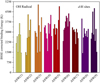 |
Fig. 1 BSSE-corrected BE values of all 75 d-H positions for the nine different ASW [H2O]20 clusters. The corresponding values are presented in Table A.2 (available on Zenodo). |
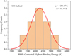 |
Fig. 2 Gaussian distribution for the highest BE values of the OH radicals over the highest d-H binding sites for the nine ASW [H2O]20 clusters. |
BSSE-corrected (+) and uncorrected (−) BEs for different radicals for the ASW(1) [H2O]20 cluster.
3.2 BSSE correction
The BSSE is intuitively a highly plausible concept. The BSSE correction using the CPC method accounts for the superposition error caused by the sloppy treatment of the basis set for each monomer of a big cluster, as the intermolecular distance varies. Even if this inconsistency could be eradicated entirely, errors related to the incompleteness of the basis set, known as the basis set completeness error (BSCE), would remain. Hypothetically, the BSSE and the BSCE would be zero in the complete basis set limit. The BSSE and BSCE often have opposite signs (Dunning 2000). For small and medium basis sets around the van der Waals minimum, the (negative) BSCE cancels (part of) the (positive) BSSE (Sheng et al. 2011). Ignoring one basis set fault while accounting for the other can produce imbalanced results. According to Sheng et al. (2011), diffuse basis functions can help reduce the BSSE. However, they also pointed out that diffuse basis functions can reduce the BSCE. Therefore, the partial cancelation of these errors still applies, and the extensive use of diffuse basis functions does not lead to a different conclusion. Jensen (2024) recently pointed out that the most significant source of error for smaller basis sets is the BSCE. Furthermore, he noted that these errors are dominant in dispersion-type interactions and that including CPC can, in such cases, lead to a deterioration of the results.
The recent studies by Perrero et al. (2022), Bovolenta et al. (2022), and Tinacci et al. (2023) suggest that BE values can be erroneous for bigger systems without BSSE correction. Considering these contradictory statements, and to reduce the computational cost and make the calculations possible, we used only one small basis set, 6-311+G(d,p), and thus cannot extrapolate toward the complete basis set limit. Hence, we relied on an estimate to determine the influence of the BSSE on the highest physisorption BEs of the radicals.
In Table 3 we compare the BE results obtained by carrying out BSSE correction using the CPC method and the BSSE-uncorrected BE for the d-H binding sites with the highest BE found for all seven radicals with the ASW(1) cluster. It is to be noted that for the CH radical, the highest BEs are due to the chemisorption process (see Table A.3, available on Zenodo). Chemisorption refers to the formation of a chemical bond between two atoms of the radical and water cluster. The structural geometries (see Fig. A.3, available on Zenodo) suggest that for the CH radical, the cluster geometries get broken, and consequently, CH2OH and CHOH+H formation happens at sites 5 and 7 of the ASW(1) cluster, respectively. This is similar to the case found for C and CH in Wakelam et al. (2017), Shimonishi et al. (2018), and Molpeceres et al. (2021). We considered the highest BE value among only the physisorbed energy values for the sake of calculation consistency. The result is less evident for the CN radical (an exceptionally large BSSE-corrected BE of 6317 K at site 5 in the ASW(1) cluster) as no structural change can be seen. It is thought that CN forms a nonclassical 2c-3e bond (a hemibond) between the unpaired electron on the CN carbon atom and the lone pair of electrons of the oxygen atom of the water surface instead of forming H bonds with the surface (Rimola et al. 2018; Martínez-Bachs et al. 2024) and is most probably the reason for the significantly large BE value. For the case of CN, we considered 1086 K as the highest BSSE-corrected BE value for consistency. To better understand the dependence of the BSSE on the BE, the BSSE-corrected and uncorrected BEs are plotted side by side in Fig. 3 and compared with the ratio by which the BSSE-corrected BEs are lower than the uncorrected one for all seven radicals. From Table 3, we see that the average ratio is ≈ 1.179, considering the d-H binding sites with the highest BE found for all seven radicals with the ASW(1) cluster. A quantitative study on the BSSE dependence of the OH radical taking all the binding sites in the ASW(1) cluster into consideration was also performed (see Table A.4, available on Zenodo). The BSSE-corrected and uncorrected values and the uncorrected-to-corrected ratio are plotted in Fig. A.4 (available on Zenodo). The average uncorrected-to-corrected ratio for OH is ≈ 1.119. The BE values with BSSE adjustments are consistently lower than those without BSSE corrections for all cases. Unless otherwise stated, all BEs discussed hereafter are BSSE-corrected BEs.
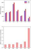 |
Fig. 3 Bar plots for BSSE-corrected (+) and uncorrected (−) highest BE values (upper panel) and the ratio between the uncorrected and corrected BE values (lower panel) for seven radicals. |
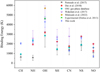 |
Fig. 4 Comparison of the BEs computed in the present work (blue stars) and those based on the available literature and frequently used databases noted in Table 2. The solid lines go from the minimum to the maximum BE values for each species. Only the OH radical has reported experimental data (green circle). The dashed gray vertical lines guide the eye to identify the corresponding species. |
3.3 Comparison of the BEs with previous studies
The experimental investigation of radical binding properties is complex since, during the heating ramp of conventional temperature programmed desorption, the radical has an enormous chance to diffuse and react, making the experimental evaluation of the desorption parameters almost impossible. The obtained BE values depend strongly on the chemical composition and morphology of the substrate, as well as the monolayer or multilayer regime used in the experiment (He et al. 2016). To the best of our knowledge, no experimental studies have provided the BEs of the radicals considered in this study, except for a handful of experimental determinations for the BE of OH on amorphous silicate surfaces. Therefore, we do not have many constraints to benchmark our computed values. Moreover, comparing the theoretical BEs with experimentally determined ones is not straightforward. We must, therefore, rely on existing theoretical reference values. In Table 2 we compare our calculated BE with other available experimental, computational, and public database values. To better visualize the comparison, we plot all the tabulated data on a common diagram in Fig. 4. To use a coherent set of homogeneous data for comparison, we chose the BE values recommended by (Das et al. 2018, except for CH) and Penteado et al. (2017) and used the KInetic Database for Astro-chemistry (KIDA) for many of the radicals. Penteado et al. (2017) present a list of the recommended BEs, which includes data from previous studies and an uncertainty range for each value. The uncertainty assigned is set to half the BE for species with less than 1000 K (CH and NH) and 500 K for all other cases (SH, CN, NS, and NO). For all the radicals considered here except OH, the provided average BEs are based on the work of Hasegawa & Herbst (1993) and Aikawa et al. (1996).
OH: the binding properties of the OH radical are difficult to study experimentally due to its tendency to diffuse and react, leading to the formation of ASW on the bare surface during conventional temperature programmed desorption heating ramps. Only a couple of existing experimental studies have reported the BE for hydroxyl radical on bare amorphous silicates: 4600 K (Dulieu et al. 2013) and 1656-4760 K (He & Vidali 2014). Penteado et al. (2017) later recommended BE = 3210 ± 1550 K, based on the distribution determined by He & Vidali (2014), taking the average with uncertainty to cover this range. However, as far as we know, no experimental study considering ASW surfaces has been published to date. Several other existing reference values are available for OH. The Ohio State University (OSU) gas-phase database gives 2850 K, assuming half the value of H2O (Garrod & Herbst 2006). A systematic empirical approach by Wakelam et al. (2017) provided 4600 ± 1380 K using the [H2O]1 ASW model. Das et al. (2018), using quantum calculations and the [H2O]4 ASW model, find 3183 K. Ferrero et al. (2020) determined the range 1816-6230 K using the amorphous 2D slab ice model, generated from the [H2O]20 structures from Shimonishi et al. (2018). There are some estimated average values ranging between 4300 K (considering both crystalline and ASW substrates; Miyazaki et al. 2020) and 4990 K (between 2321 and 7770 K on top of a crystalline water ice; Sameera et al. 2017). Duflot et al. (2021) find an average best estimate of 5199 ± 1938 K between minimum 2936 K and maximum 8924 K for the amorphous ice model. Enrique-Romero et al. (2022) calculated 2911 and 5376 K for the [H2O]18 and [H2O]33 ASW ice models. Finally, after examining the available studies, Minissale et al. (2022) recommended a value of 5698 K. Very recently, Hendrix et al. (2023) computed the BEs of OH to the H2O monomer, dimer, trimer, and tetramer as 1922, 3900, 4252, and 3674 K, respectively, using the CCSD(T)/aug-cc-pVTZ level of theory and 1907, 3905, 4433, and 3840 K, respectively, using the DFT-ωB97X-V/def2-qzvppd level of theory. They noticed that the H-bond distances between the O atom of OH and the H atom of H2O shorten notably when an H2O molecule is added to the cluster. As shown in Fig. 4, our calculated average BE of 4287 ± 566 K is well within the range of existing experimental, theoretical, and recommended values, and is close to the central value.
CH: as per our knowledge, no computational or experimental BE value exists for the methylidyne (also called carbyne) radical to date. Wakelam et al. (2017) attempted to consider CH in their work but noticed the formation of strong (partly) covalent bonding with a single H2O molecule. However, they did not provide any chemisorption value. We calculated its BE considering seven d-H sites of the ASW(1) [H2O]20 cluster (see Table A.3, available on Zenodo). We notice that two d-H sites favor chemisorption (see Fig. A.3, available on Zenodo), whereas the other five sites favor physisorption. The C–H chemical bond lengths of 1.372 and 1.513 Å (which are longer than the typical covalent bond length of 1.08 Å) are formed at these two chemisorption binding sites. A recent study by Nguyen & Peeters (2021) on the reaction rate of CH with H2O vapor suggests that in the reaction pathway, the first step is the barrierless association leading to a pre-reactive complex, which has a BE of 8.93 kcal mol−1 (~4494 K). This pre-reactive complex (HCδ+−δ−OH2) is formed via a polar interaction between a lone pair orbital of the O atom and an empty p-orbital of the C atom. Subsequently, the pre-reactive complex can isomerize to CH2OH if CH is inserted into an O–H bond of H2O. A similar chemisorp-tion behavior of a C atom with H2O was recognized by previous studies (Wakelam et al. 2017; Shimonishi et al. 2018; Molpeceres et al. 2021). The large dipole moment (1.46 D; Phelps & Dalby 1966) could be the reason for the strong long-range interaction, which would mean it is reactive to neutral H2O molecules. As seen from Table 2 and Fig. 4, our proposed average BE of 2044 ± 94 K is higher than the estimated range of 590 ± 295 K (based on educated guesses) provided in Penteado et al. (2017), as well as the 925 K provided by the OSU gas-phase database. To clarify, our average BE was calculated without taking the chemisorbed BE values into account (see Table A.3, available on Zenodo).
NH: we report an average BE for imidogen, or nitrene, of 2234 ± 178 K, which is in good agreement with the OSU database value of 2378 K and within the range 2600 ± 780 K proposed by Wakelam et al. (2017). Our calculated value is well above the recommended value of 542 ± 270 K (Penteado et al. 2017) and higher than the value of 1947 K computed by Das et al. (2018). Martínez-Bachs et al. (2020) report BEs of 4222 K for a crystalline water-ice surface. Our value agrees well with the best-estimated average value of 2437 ± 1126 K for the amorphous ice model (Duflot et al. 2021). Enrique-Romero et al. (2022) recently calculated the BEs of NH as 1560 and 3909 K on the [H2O]18 and [H2O]33 ASW ice models, respectively, considering a single binding site; this is a simplistic assumption given that different surface binding sites are available and, accordingly, a distribution of BEs exists. Enrique-Romero et al. (2022) also noted (from the private communication with B. Martinez-Bachs) the BE range 1320-5410 K for ASW ice surfaces, centered at around 2410 K. However, the very recent calculations by Martínez-Bachs et al. (2024) show a range of BEs for the ASW model, varying from a minimum of 1167 K to a maximum of 4692 K, with an average of 2464 K, which is also in close agreement with our value.
SH/HS: we report the average BE for mercapto, or the sul-fanyl radical, as 2482 ± 314 K, which is within the range 2600 ± 780 K proposed by Wakelam et al. (2017). However, the other values – 1450 K (OSU database), 1350 ± 500 K (Penteado et al. 2017), 2221 K (Das et al. 2018), and 2195 ± 931 K (Perrero et al. 2022) – are somewhat lower than our computed average value.
CN: our computed average BE value for the cyano radical (1278 ± 41 K) is consistent with the existing values of 1600 K (OSU database), 1355 ± 500 K (Penteado et al. 2017), and 1736 K (Das et al. 2018), but not with the larger value of 2800 ± 840 K proposed by Wakelam et al. (2017). However, an exceptionally high BE of 6317 K is found for site 5 in the ASW(1) [H2O]20 cluster. This value was not included in the average calculation. This high BE value coincides with the range of BEs proposed by Martínez-Bachs et al. (2024): 2605 K to 7792 K, with an average of 4856 K. The hemibond nature is most probably the reason for this inconsistency.
NS: unlike the case of the CH radical, our calculated average BE for the nitrogen monosulfide radical, 2619 ± 198 K, is higher than the available estimated range of 1800 ± 500 K (Penteado et al. 2017), as well as the 1900 K provided by the OSU gas-phase database. The value of 2774 K calculated by Das et al. (2018) is somewhat close to our calculated average value. Perrero et al. (2022) calculated an average BE of 2026 K, a minimum of 1234 K, and a maximum of 2955 K for an amorphous ice model.
NO: our computed average BE value of 704 ± 94 K for the nitric oxide radical is well within the range 1085 ± 500 K proposed by Penteado et al. (2017) as well as the range calculated by Das et al. (2018) for a different ASW ice model (568–1988 K).
The KIDA database suggests a higher value of 1600 ± 480 K as proposed by Wakelam et al. (2017). Very recently, Hendrix et al. (2023) computed the BEs of the NO to H2O monomer, dimer, trimer, and tetramer as 367, 1147, 438, and 1354 K, respectively, using the CCSD(T)/aug-cc-pVTZ level of theory and 252, 1022, 649, and 1087 K using the DFT-ωB97X-V/def2-qzvppd level of theory. Similar to NH, the results of Martínez-Bachs et al. (2024) give an energy range of 291-965 K, with an average of 712 K, which strongly agrees with our results. The low BE of NO on the surface is primarily governed by dispersive interactions. This is due to the almost negligible dipole moment of NO, which limits the contribution of electrostatic interactions to the overall binding.
It is important to note that the small fluctuations observed in the calculated BEs compared to literature values can be attributed to several factors, including the specific computational method employed, the adopted ice model, and the particular binding sites investigated in this study. Open-shell species pose significant computational challenges due to multi-reference characteristics and the need to account for static and dynamic correlation effects. Accurately capturing the true energy of these species requires a sensitive and careful approach, often involving multi-reference wave function theories (e.g., the coupled cluster method) and perturbation methods (e.g., the Møller-Plesset method). Although these techniques can provide highly accurate results, they come with a substantial computational cost. The combination of the ωB97X-D functional and the 6-311+G(d,p) basis set offers a practical balance between accuracy and efficiency. The ωB97X-D functional is crucial for handling the complex electronic structures inherent to radicals and is a versatile tool for studying a wide range of systems. The 6-311+G(d,p) basis set, with its valence triple-ζ quality and added polarization functions, further enhances the accuracy by providing a flexible and detailed description of electron density, especially where electron distribution is uneven due to unpaired electrons. This combination is not necessarily the best or most accurate option available. Still, it is a well-considered choice that delivers a high degree of accuracy while keeping computational costs relatively low. Furthermore, we believe that our methodology, with careful structural optimization and analysis, is robust enough to be applied to other radical species and, more generally, to species with challenging electronic structures.
4 Astrophysical implications
It is crucial to comprehend the impact of the newly computed BEs on interstellar ice chemistry, as some of them differ from the values used in the past few decades. We outline the implications of these computed values below.
4.1 Chemisorption
Some of our binding sites exhibit chemisorption for CH (a chemical bond is formed with one oxygen atom of a water molecule of the cluster). Figure A.3 (available on Zenodo) depicts the formation of CH2OH and CHOH2 by chemisorption. There is a possibility that the chemisorbed CH2OH could produce CH3OH via the Eley-Rideal mechanism by capturing an H atom from the gas phase. Alternatively, a chemisorbed H atom could react with CH2OH to form methanol. Recent experiments by Grieco et al. (2024) suggest the formation of H2O at a high temperature (approximately 85 K) by chemisorbed H and O. Additionally, Grieco et al. (2023) reported the formation of H2 up to a temperature as high as 250 K, suggesting the feasibility of hydrogenation reactions at higher temperatures than previously thought. Contrary to previous understandings of methanol formation through the surface hydrogenation of CO, Molpeceres et al. (2021) and Tsuge et al. (2023) suggest that before CO freeze-out, atomic carbon deposited on ASW could form H2CO. Tsuge et al. (2023) pointed out that at temperatures below 20 K, some of the accreted carbon atoms are quickly converted to formaldehyde. The remaining physisorbed atoms are partially changed to chemisorbed and hydrogenated to CH4. Physisorbed carbon atoms can diffuse at temperatures between 20 and 30 K, promoting insertion reactions with other carbon atoms or species. Future observations with the James Webb Space Telescope (JWST) could provide additional details about the significance of chemisorption in forming complex organic molecules in the ice phase.
4.2 Implication of the computed BEs for the astrochemical model
Recently, using Atacama Large Millimeter/submillimeter Array (ALMA) observations, Coutens et al. (2019) detected multiple transitions of HONO in the low-mass protostellar system IRAS 16293–2422. This system consists of three protostars, two located toward source A and one toward source B (Maureira et al. 2020). The identification by Coutens et al. (2019) specifically focuses on the protostar associated with source B. They also attempted to explain the abundances of HONO-related species and their ratios using a chemical model. However, they were unable to account for all the observed features. In their study, Coutens et al. (2019) estimated abundance ratios of HONO/NH2OH and HONO/HNO to be greater than or equal to 2.3 and 3, respectively. Using their chemical model, they successfully explain the abundance of HONO, N2O, and NO2. However, their model resulted in an overproduction of NH2OH and HNO, leading to lower HONO/NH2OH (1.7 × 10⁻³) and HONO/HNO (0.01) ratios compared to the observed values. Our study suggests a weak binding of NO with the water substrate. It would be interesting to see how the estimated BEs would affect the modeled abundances of these species.
We utilized the Rokko code Furuya et al. (2015, 2017) for our chemical modeling, which encompasses three phases: gas, icy grain surface, and homogeneous bulk ice mantle. Our active ice layers were limited to the top four monolayers. All layers, including the active ice layers, were considered part of the bulk ice mantle. The gas- and ice-phase networks are based on the work of Garrod (2013). The active layers undergo photodissoci-ation and the photo-desorption of species. A constant reactive desorption of all the species by a factor of 0.01 is assumed, resulting in a single product. MD studies have determined that approximately 10% of the formation energy is retained after the formation of H2S from HS+H (Bariosco et al. 2024, and references therein). However, based on experimentally determined reaction desorption probabilities for H2S, HDS, and D2S (Oba et al. 2019; Furuya et al. 2022), we used a reactive desorption factor of 0.03. We also used a standard cosmic-ray ionization rate of 1.3 × 10⁻¹⁷ s−1.
4.2.1 Dark cloud
For the dark cloud model, we started with a hydrogen number density, nH= 2 × 104 cm−3, a visual extinction (AV) of 10 mag, and a gas and ice temperature of 10 K. The initial elemental abundances of species were taken from Garrod et al. (2017). The upper panel of Fig. 5 shows the time evolution of the radicals. Here, “G” indicates that all the BE sets are from Garrod (2013); “G+S” indicates that the BEs for the radicals are taken from this work and the other BEs from Garrod (2013). In this work we used a default diffusion-to-BE ratio of 0.4. Since no estimated BEs were available for HONO, H2NO2, and H3NO2, we used our estimated values of 2918, 4205, and 3044 K, respectively, in both “G” and “G+S”. Changes in the BE would have a minor effect on the gas-phase abundances of these radicals. However, they would have a major effect on the ice-phase abundances of these radicals, especially for the ice-phase NO and CH. The NO ice abundance is reduced by a factor of almost 105 at 106 years. Meanwhile, the ice-phase abundance of CH increases by a factor of 100. The reduction in the abundance of NO is due to the weak binding of NO obtained in this work (~704 K) compared to the earlier estimate (1600 K; Wakelam et al. 2017). The increase in the surface abundance of CH radicals is due to the higher estimated BE (~2044 K) compared to previous work (Garrod 2013, 925 K). The shaded lines on the graph indicate the uncertainty of our BE values from Table 2. Since NO has a very weak binding with the water substrate, its low uncertainty (about 94 K) in the BE estimation could cause a significant change in its ice-phase abundance (see the black shaded area in the top right panel of Fig. 5).
The lower panel of Fig. 5 presents the time evolution of the NO-related species. It clearly shows that with the present BE estimation of NO, we can expect a favorable formation of gas-phase HONO in a dark cloud. On the contrary, the formation of gas-phase NH2OH is heavily affected, which could be useful in explaining the observed HONO/NH2OH ratio in star-forming regions (Coutens et al. 2019) discussed in Sect. 4.2.2. The shaded regions are the results when the uncertainty in the BE calculations is taken into consideration. The obtained abundances and abundance ratio with HONO are noted in Table 4. Due to the weak binding of NO obtained in this study, we find a higher abundance of the ice-phase NO2 through the reaction NO − gr + O − gr → NO2 − gr, which results in a favorable formation of HONO−gr by H − gr + NO2 − gr → HONO − gr. The formation of NH2OH-gr occurs through successive hydrogenation reactions:  . When our BE value of NO is used, due to the high abundance of atomic oxygen on the grain compared to the atomic hydrogen, NO-gr is mainly channelized to form NO2 − gr, resulting in a decrease in the formation of NH2OH − gr. On the contrary, it facilitates the HONO-gr formation. The lower panel of Fig. 5 presents the observed significant uncertainties in the ice−phase abundances of HNO and NH2OH due to the uncertainty surrounding the BE of NO (~94 K).
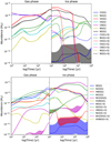 |
Fig. 5 Changes in the abundances of gas- and ice-phase radicals over time in a dark cloud. The solid lines represent the results obtained using the BE values from Garrod (2013, “G”), while the dashed curves represent the results obtained using our calculated BE values (“G+S”). The filled curve around the calculated BE curves shows the abundances when the errors on the calculated BEs are taken into account, as presented in Table 2. |
Peak abundances and abundance ratios for NO-related species obtained from our model and a comparison of peak abundance ratios with the available observation.
4.2.2 Hot corino
We further examined a low-mass star-forming region to assess the impact of our proposed BEs on abundance estimations. We considered three stages: the isothermal collapsing stage, the warm−up stage, and the post-warm-up stage. During the isothermal collapsing stage, the cloud was allowed to collapse from a minimum density of nmin = 3 × 103 cm−3 to a maximum density of nmax = 107 cm−3 in 1 million years, with a constant gas temperature of 10 K and an ice temperature of 10 K. The initial abundance for this model was taken from the final abundance of the dark cloud model discussed in Sect. 4.2.1. The visual extinction in the first stage was allowed to vary with the density following the relation provided by Garrod & Pauly (2011), resulting in a variation of AV = 2−446. In the warm-up stage, the density and visual extinction parameters were consistently set to their maximum values for an additional 1 million years, and the temperature gradually rose to a peak of ~200 K. During the post-warm-up stage, the parameters listed above remained at their maximum values for an additional 105 years.
The upper panel of Fig. 6 shows the time evolution of the abundances of gas-phase radicals. With the new BE value, the gas-phase abundance of NO (dashed black curve) decreases significantly during the warm-up stage. In the lower panel of Fig. 6, we show the abundances of NO and its related species separately. The uncertainties in the BE calculations are also considered here as discussed in the context of Fig. 5. In Table 4, we compare the peak abundances (peak value is taken beyond the isothermal stage) and the peak abundance ratio of some NO−related species obtained from our simulations with that observed by Coutens et al. (2019). With the new BEs (represented by the dashed curves), we observe a significant reduction in the abundances of NO, N2O, HNO, and NH2OH. Conversely, there is a surge in the abundance of HONO.
NH2OH is primarily produced in the cold ice phase through the successive sequential hydrogenation of NO-gr, as discussed in Sect. 4.2.1, and it can sublimate to the gas phase after around 1.7 × 10⁶ years, depending on the BE (6806 K; Garrod 2013). Due to the weak binding of NO, its abundance in the ice phase decreases as it forms NO2, leading to a decrease in NH2OH. We estimate a BE of 2918 K for HONO, so it is expected to be released earlier than NH2OH in the gas phase. However, an additional radical-radical pathway (OH − gr + NO − gr → HONO − gr) is responsible for ice− phase HONO production in warmer regions. The low BE of NO obtained here further facilitates this radical-radical ice-phase reaction.
In our study, with our estimated BE for NO, we obtain a lower abundance of NH2OH and HNO (see Fig. 6 and Table 4). We obtain peak abundance ratios of HONO/NH2OH and HONO/HNO of 143 and 3781, respectively, consistent with the observation. Table 4 shows that the other ratios from the observations seem to be between that found using the previous model (Coutens et al. 2019) and this model. This may indicate that the diffusion activation energy of NO was overestimated in the previous one and underestimated in the present.
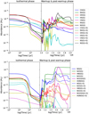 |
Fig. 6 Time evolution of the abundances of gas-phase NO-related species in the hot core. Solid lines represent the BE used from Garrod (2013, “G”), and dashed curves when our calculated BEs are used (“G+S”). |
5 Conclusions
This study aimed to calculate the BE of certain interstellar radicals on cluster surfaces of ASW. We employed a fully quantum chemical approach to examine a large number of binding sites for all the considered radicals using a suitable ASW cluster model. The significant findings of our work are as follows:
We estimated the BEs of seven diatomic radicals using a pure quantum chemical approach with high-level water clusters and methods, and we discuss the implications of the computed BEs for astrochemical models.
We carefully and extensively employed the BSSE correction using the CPC method. This correction is crucial, especially with small and medium-sized basis sets, for obtaining accurate and reliable estimates of the BEs between radical species and the ASW cluster.
Our results suggest that, most of the time, we have physisorption, indicating weak bonding between radicals and the water molecule. However, in addition to physisorption, we find chemisorption of CH with the [H2O]20 cluster in two cases. In these cases, a chemical bond is formed between CH and an oxygen atom of a water molecule. Figure A. 3 (available on Zenodo) illustrates the production of CH2OH through the chemisorption of CH on a water substrate. This warrants the potential formation of methanol through hydrogenation in warmer regions. Future observations with the JWST could address this issue. Moreover, our estimated value of the BE (physisorption) of CH is 2–3 times higher than the available estimate. Hence, we suggest using these values for astrochemical models.
We obtain a significantly lower BE value of NO (704 K), which is in excellent agreement with a very recent study (average value of 712 K with the ASW model; Martínez-Bachs et al. 2024) compared to that used earlier (1600 K). Our obtained BEs of NO can help explain the observed HONO/NH2OH and HONO/HNO ratio obtained in the B component of the low-mass protostellar binary IRAS 16293–2422.
Data availability
The data underlying this article (in the appendix) are made available under a Creative Commons Attribution license on Zenodo: doi:10.5281/zenodo.13388691.
Acknowledgements
The authors thank the anonymous referee for the valuable insights and constructive comments that significantly improved the manuscript. M.S. acknowledges financial support through the European Research Council (consolidated grant COLLEXISM, grant agreement ID: 811363). N.I. acknowledges the support of FONDECYT Regular Grant 1241193 and Vicerectoría de Investigación y Postgrado (VRIP). A.D. acknowledges the support of MPE for sponsoring a scientific visit to MPE.
References
- Aikawa, Y., Miyama, S. M., Nakano, T., & Umebayashi, T. 1996, ApJ, 467, 684 [NASA ADS] [CrossRef] [Google Scholar]
- Bariosco, V., Pantaleone, S., Ceccarelli, C., et al. 2024, MNRAS, 531, 1371 [NASA ADS] [CrossRef] [Google Scholar]
- Boogert, A. C. A., Gerakines, P. A., & Whittet, D. C. B. 2015, ARA&A, 53, 541 [Google Scholar]
- Bovolenta, G., Bovino, S., Vöhringer-Martinez, E., et al. 2020, Mol. Astrophys., 21, 100095 [NASA ADS] [CrossRef] [Google Scholar]
- Bovolenta, G. M., Vogt-Geisse, S., Bovino, S., & Grassi, T. 2022, ApJS, 262, 17 [NASA ADS] [CrossRef] [Google Scholar]
- Boys, S., & Bernardi, F. 1970, Mol. Phys., 19, 553 [NASA ADS] [CrossRef] [Google Scholar]
- Chai, J.-D., & Head-Gordon, M. 2008, Phys. Chem. Chem. Phys., 10, 6615 [NASA ADS] [CrossRef] [Google Scholar]
- Coutens, A., Ligterink, N. F. W., Loison, J.-C., et al. 2019, A&A, 623, L13 [NASA ADS] [CrossRef] [EDP Sciences] [Google Scholar]
- Das, A., & Chakrabarti, S. K. 2011, MNRAS, 418, 545 [CrossRef] [Google Scholar]
- Das, A., Acharyya, K., Chakrabarti, S., & Chakrabarti, S. K. 2008, A&A, 486, 209 [NASA ADS] [CrossRef] [EDP Sciences] [Google Scholar]
- Das, A., Acharyya, K., & Chakrabarti, S. K. 2010, MNRAS, 409, 789 [NASA ADS] [CrossRef] [Google Scholar]
- Das, A., Majumdar, L., Sahu, D., et al. 2015, ApJ, 808, 21 [NASA ADS] [CrossRef] [Google Scholar]
- Das, A., Sahu, D., Majumdar, L., & Chakrabarti, S. K. 2016, MNRAS, 455, 540 [NASA ADS] [CrossRef] [Google Scholar]
- Das, A., Sil, M., Gorai, P., Chakrabarti, S. K., & Loison, J. C. 2018, ApJS, 237, 9 [NASA ADS] [CrossRef] [Google Scholar]
- Das, A., Gorai, P., & Chakrabarti, S. K. 2019, A&A, 628, A73 [NASA ADS] [CrossRef] [EDP Sciences] [Google Scholar]
- Das, A., Sil, M., Ghosh, R., et al. 2021, Front. Astron. Space Sci., 8, 78 [NASA ADS] [CrossRef] [Google Scholar]
- Duflot, D., Toubin, C., & Monnerville, M. 2021, Front. Astron. Space Sci., 8, 24 [NASA ADS] [CrossRef] [Google Scholar]
- Dulieu, F., Congiu, E., Noble, J., et al. 2013, Sci. Rep., 3, 1338 [Google Scholar]
- Dunning, T. H. 2000, J. Phys. Chem. A, 104, 9062 [CrossRef] [Google Scholar]
- Enrique-Romero, J., Rimola, A., Ceccarelli, C., et al. 2022, ApJS, 259, 39 [NASA ADS] [CrossRef] [Google Scholar]
- Ferrero, S., Zamirri, L., Ceccarelli, C., et al. 2020, ApJ, 904, 11 [NASA ADS] [CrossRef] [Google Scholar]
- Frisch, M. J., Trucks, G. W., Schlegel, H. B., et al. 2009, Gaussian 09 Revision A.01 (Wallingford CT: Gaussian Inc.) [Google Scholar]
- Frisch, M. J., Trucks, G. W., Schlegel, H. B., et al. 2013, Gaussian 09 Revision D.01 (Wallingford CT: Gaussian Inc.) [Google Scholar]
- Frisch, M. J., Trucks, G. W., Schlegel, H. B., et al. 2016, Gaussian 16 Revision B.01 (Wallingford CT: Gaussian Inc.) [Google Scholar]
- Frisch, M. J., Trucks, G. W., Schlegel, H. B., et al. 2019, Gaussian 16 Revision C.01 (Wallingford CT: Gaussian Inc.) [Google Scholar]
- Furuya, K., Aikawa, Y., Hincelin, U., et al. 2015, A&A, 584, A124 [NASA ADS] [CrossRef] [EDP Sciences] [Google Scholar]
- Furuya, K., Drozdovskaya, M. N., Visser, R., et al. 2017, A&A, 599, A40 [NASA ADS] [CrossRef] [EDP Sciences] [Google Scholar]
- Furuya, K., Oba, Y., & Shimonishi, T. 2022, ApJ, 926, 171 [NASA ADS] [CrossRef] [Google Scholar]
- Garrod, R. T. 2013, ApJ, 765, 60 [Google Scholar]
- Garrod, R. T., & Herbst, E. 2006, A&A, 457, 927 [NASA ADS] [CrossRef] [EDP Sciences] [Google Scholar]
- Garrod, R. T., & Pauly, T. 2011, ApJ, 735, 15 [Google Scholar]
- Garrod, R. T., Widicus Weaver, S. L., & Herbst, E. 2008, ApJ, 682, 283 [Google Scholar]
- Garrod, R. T., Belloche, A., Müller, H. S. P., & Menten, K. M. 2017, A&A, 601, A48 [NASA ADS] [CrossRef] [EDP Sciences] [Google Scholar]
- Germain, A., Tinacci, L., Pantaleone, S., Ceccarelli, C., & Ugliengo, P. 2022, ACS Earth Space Chem., 6, 1286 [Google Scholar]
- Ghosh, R., Sil, M., Kumar Mondal, S., et al. 2022, Res. Astron. Astrophys., 22, 065021 [CrossRef] [Google Scholar]
- Gibb, E. L., Whittet, D. C. B., Boogert, A. C. A., & Tielens, A. G. G. M. 2004, ApJS, 151, 35 [NASA ADS] [CrossRef] [Google Scholar]
- Grieco, F., Theulé, P., De Looze, I., & Dulieu, F. 2023, Nat. Astron., 7, 541 [NASA ADS] [CrossRef] [Google Scholar]
- Grieco, F., Dulieu, F., De Looze, I., & Baouche, S. 2024, MNRAS, 527, 10604 [Google Scholar]
- Hama, T., & Watanabe, N. 2013, Chem. Rev., 113, 8783 [Google Scholar]
- Hasegawa, T. I., & Herbst, E. 1993, MNRAS, 261, 83 [NASA ADS] [CrossRef] [Google Scholar]
- Hasegawa, T. I., Herbst, E., & Leung, C. M. 1992, ApJS, 82, 167 [Google Scholar]
- He, J., & Vidali, G. 2014, ApJ, 788, 50 [Google Scholar]
- He, J., Acharyya, K., & Vidali, G. 2016, ApJ, 825, 89 [Google Scholar]
- Hendrix, J., Bera, P. P., Lee, T. J., & Head-Gordon, M. 2023, Mol. Phys., 0, e2252100 [Google Scholar]
- Ioppolo, S., Fedoseev, G., Chuang, K. J., et al. 2021, Nat. Astron., 5, 197 [NASA ADS] [CrossRef] [Google Scholar]
- Jensen, F. 2024, J. Chem. Theor. Comput., 20, 767 [CrossRef] [Google Scholar]
- Jin, M., & Garrod, R. T. 2020, ApJS, 249, 26 [Google Scholar]
- Keane, J. V., Tielens, A. G. G. M., Boogert, A. C. A., Schutte, W. A., & Whittet, D. C. B. 2001, A&A, 376, 254 [NASA ADS] [CrossRef] [EDP Sciences] [Google Scholar]
- Martínez-Bachs, B., Ferrero, S., & Rimola, A. 2020, in Computational Science and Its Applications – ICCSA 2020, eds. O. Gervasi, B. Murgante, S. Misra, et al. (Cham: Springer International Publishing), 683 [CrossRef] [Google Scholar]
- Martínez-Bachs, B., Ferrero, S., Ceccarelli, C., Ugliengo, P., & Rimola, A. 2024, ApJ, 969, 63 [CrossRef] [Google Scholar]
- Maureira, M. J., Pineda, J. E., Segura-Cox, D. M., et al. 2020, ApJ, 897, 59 [NASA ADS] [CrossRef] [Google Scholar]
- McGuire, B. A. 2022, ApJS, 259, 30 [NASA ADS] [CrossRef] [Google Scholar]
- Minissale, M., Aikawa, Y., Bergin, E., et al. 2022, ACS Earth Space Chem., 6, 597 [NASA ADS] [CrossRef] [Google Scholar]
- Miyazaki, A., Watanabe, N., Sameera, W. M. C., et al. 2020, Phys. Rev. A, 102, 052822 [NASA ADS] [CrossRef] [Google Scholar]
- Molpeceres, G., Kästner, J., Fedoseev, G., et al. 2021, J. Phys. Chem. Lett., 12, 10854 [CrossRef] [Google Scholar]
- Mondal, S. K., Gorai, P., Sil, M., et al. 2021, ApJ, 922, 194 [NASA ADS] [CrossRef] [Google Scholar]
- Nguyen, T. L., & Peeters, J. 2021, Phys. Chem. Chem. Phys., 23, 16142 [NASA ADS] [CrossRef] [Google Scholar]
- Oba, Y., Tomaru, T., Kouchi, A., & Watanabe, N. 2019, ApJ, 874, 124 [NASA ADS] [CrossRef] [Google Scholar]
- Penteado, E. M., Walsh, C., & Cuppen, H. M. 2017, ApJ, 844, 71 [Google Scholar]
- Perrero, J., Enrique-Romero, J., Ferrero, S., et al. 2022, ApJ, 938, 158 [NASA ADS] [CrossRef] [Google Scholar]
- Phelps, D. H., & Dalby, F. W. 1966, Phys. Rev. Lett., 16, 3 [Google Scholar]
- Piacentino, E. L., & Öberg, K. I. 2022, ApJ, 939, 93 [NASA ADS] [CrossRef] [Google Scholar]
- Rimola, A., Skouteris, D., Balucani, N., et al. 2018, ACS Earth Space Chem., 2, 720 [Google Scholar]
- Sameera, W. M. C., Senevirathne, B., Andersson, S., Maseras, F., & Nyman, G. 2017, J. Phys. Chem. C, 121, 15223 [CrossRef] [Google Scholar]
- Sameera, W. M. C., Senevirathne, B., Andersson, S., et al. 2021, J. Phys. Chem. A, 125, 387 [NASA ADS] [CrossRef] [Google Scholar]
- Sheng, X. W., Mentel, L., Gritsenko, O. V., & Baerends, E. J. 2011, J. Comput. Chem., 32, 2896 [CrossRef] [Google Scholar]
- Shimonishi, T., Nakatani, N., Furuya, K., & Hama, T. 2018, ApJ, 855, 27 [Google Scholar]
- Shingledecker, C. N., Vasyunin, A., Herbst, E., & Caselli, P. 2019, ApJ, 876, 140 [Google Scholar]
- Sil, M., Gorai, P., Das, A., Sahu, D., & Chakrabarti, S. K. 2017, Euro. Phys. J. D, 71, 45 [NASA ADS] [CrossRef] [Google Scholar]
- Sil, M., Gorai, P., Das, A., et al. 2018, ApJ, 853, 139 [NASA ADS] [CrossRef] [Google Scholar]
- Sil, M., Srivastav, S., Bhat, B., et al. 2021, AJ, 162, 119 [NASA ADS] [CrossRef] [Google Scholar]
- Srivastav, S., Sil, M., Gorai, P., et al. 2022, MNRAS, 515, 3524 [NASA ADS] [CrossRef] [Google Scholar]
- Tinacci, L., Germain, A., Pantaleone, S., et al. 2022, ACS Earth Space Chem., 6, 1514 [NASA ADS] [CrossRef] [Google Scholar]
- Tinacci, L., Germain, A., Pantaleone, S., et al. 2023, ApJ, 951, 32 [CrossRef] [Google Scholar]
- Tsuge, M., Molpeceres, G., Aikawa, Y., & Watanabe, N. 2023, Nat. Astron., 7, 1351 [NASA ADS] [CrossRef] [Google Scholar]
- Wakelam, V., Loison, J. C., Mereau, R., & Ruaud, M. 2017, Mol. Astrophys., 6, 22 [NASA ADS] [CrossRef] [Google Scholar]
- Whittet, D. 2003, Dust in the Galactic Environment (Bristol: IOP Publishing) [Google Scholar]
All Tables
BSSE-corrected (+) and uncorrected (−) BEs for different radicals for the ASW(1) [H2O]20 cluster.
Peak abundances and abundance ratios for NO-related species obtained from our model and a comparison of peak abundance ratios with the available observation.
All Figures
|
Fig. 1 BSSE-corrected BE values of all 75 d-H positions for the nine different ASW [H2O]20 clusters. The corresponding values are presented in Table A.2 (available on Zenodo). |
| In the text | |
|
Fig. 2 Gaussian distribution for the highest BE values of the OH radicals over the highest d-H binding sites for the nine ASW [H2O]20 clusters. |
| In the text | |
|
Fig. 3 Bar plots for BSSE-corrected (+) and uncorrected (−) highest BE values (upper panel) and the ratio between the uncorrected and corrected BE values (lower panel) for seven radicals. |
| In the text | |
|
Fig. 4 Comparison of the BEs computed in the present work (blue stars) and those based on the available literature and frequently used databases noted in Table 2. The solid lines go from the minimum to the maximum BE values for each species. Only the OH radical has reported experimental data (green circle). The dashed gray vertical lines guide the eye to identify the corresponding species. |
| In the text | |
|
Fig. 5 Changes in the abundances of gas- and ice-phase radicals over time in a dark cloud. The solid lines represent the results obtained using the BE values from Garrod (2013, “G”), while the dashed curves represent the results obtained using our calculated BE values (“G+S”). The filled curve around the calculated BE curves shows the abundances when the errors on the calculated BEs are taken into account, as presented in Table 2. |
| In the text | |
|
Fig. 6 Time evolution of the abundances of gas-phase NO-related species in the hot core. Solid lines represent the BE used from Garrod (2013, “G”), and dashed curves when our calculated BEs are used (“G+S”). |
| In the text | |
Current usage metrics show cumulative count of Article Views (full-text article views including HTML views, PDF and ePub downloads, according to the available data) and Abstracts Views on Vision4Press platform.
Data correspond to usage on the plateform after 2015. The current usage metrics is available 48-96 hours after online publication and is updated daily on week days.
Initial download of the metrics may take a while.