© The Authors 2025

1 Introduction

Collisionless stellar systems are commonly thought to reach equilibrium distributions via the process of violent relaxation (VR; Lynden-Bell 1967), associated with strong variations in the collective potential, happening for example during gravitational collapse or merger events (see Binney & Tremaine 2008). In practice, strong variations in the self-consistent gravitational potential Φ happening on a timescale of the order of a few crossing times $t_{\text{c}}\approx {(G\tilde{\rho })}^{-1/2}$ efficiently induce a redistribution of particles’ energies (Kandrup 1998a) that bring the system towards a nearly invariant equilibrium distribution, often dubbed quasi-stationary state (QSS; see e.g. Campa et al. 2014) in the context of long-range interactions.

Since its original inception, VR has been widely studied via a statistical mechanics approach (see e.g. Severne & Luwel 1980; Tremaine et al. 1986; Madsen 1987; Kandrup 1987; Padmanabhan 1990; Soker 1996; Nakamura 2000; Arad & Lynden-Bell 2005; Kang & He 2011; He 2013, and references therein). In particular, in the continuum idealized limit, the approach towards the QSS of the phase-space distribution function f as governed by the collisionless Boltzmann equation (CBE) is interpreted adopting different choices of coarse-graining in phase-space (see Kandrup 1998b; Dehnen 2005; Levin et al. 2014; Banik et al. 2022; Barbieri et al. 2022; Worrakitpoonpon 2024, see also Beraldo e Silva et al. 2024 and references therein for a complete discussion) to construct an effective dissipative process over a conservative dynamics. This stems from the fact that in the CBE-governed dynamics, the phase-space distribution f evolves as an incompressible fluid. Each continuum function 𝒢( f ) integrated over the accessible phase-space (usually dubbed Casimir invariant) is therefore conserved and thus any entropy in the form S = ∫ f ln f drdv does not evolve. This prevents the use of entropy maximization arguments to describe the evolution towards the microcanonical equilibrium. Recently, Beraldo e Silva et al. (2017, 2019a,b) conjectured that the continuum limit approach based on the CBE breaks down during processes of VR, and stated that the fast evolution towards meta-equilibria is also driven by what is known as chaotic instabilities. Such instabilities were conjectured to significantly depend on the number of degrees of freedom N (i.e. the number of particles in the system), even for astrophysically significant sizes of N ≈ 10¹¹, for which the use of continuum arguments is typically accepted.

The roles of discreteness effects and N-body chaos in driving the evolution of collisionless gravitating systems have been acknowledged since at least the work of Miller (1964, 1971) on the irreversibility of the N-body dynamics in small N systems. Moreover, several authors (Gurzadian & Savvidy 1986; Vesperini 1992; Goodman et al. 1993; Cerruti-Sola & Pettini 1995; Casetti et al. 2000; Hemsendorf & Merritt 2002; El-Zant 2002; Gurzadyan & Kocharyan 2009; El-Zant et al. 2019) inves-tigated the dependence of chaoticity in gravitational N-body systems as a function of the number of particles N in terms of the largest Lyapunov exponent (i.e. the rate of exponential divergence of initially nearby trajectories, Lichtenberg & Lieberman 2013). In particular, Kandrup and collaborators (Kandrup 1996; Kandrup & Sideris 2001; Sideris & Kandrup 2002; Vass et al. 2003; Kandrup & Sideris 2003; Kandrup et al. 2003; Sideris & Kandrup 2004; Kandrup & Novotny 2004) studied how the collective properties of ensembles of trajectories relate to their average maximal Lyapunov exponents when propagated in both static non-integrable or periodically pulsated galactic potentials, as well as frozen N-body models (i.e. systems composed of N fixed particles sampling a given continuum density ρ(r) and exerting a Newtonian potential, possibly softened). The main results of these studies (see e.g. Merritt 2005 for an almost complete review) can be summarized as follows:

1. The timescale of the perturbation growth of individual stellar orbits decreases as N⁻¹, as opposed to the N^1/3 scaling proposed by Gurzadian & Savvidy (1986).

2. For sufficiently large values of N, the r.m.s. of the spatial position of initially localized orbit ensembles evolves as $$\langle r\rangle \propto C(N)\exp (t/t_{\text{c}}),$$(1) where the factor C is a decreasing function of the number of degrees of freedom (i.e. the number of particles).

3. Point 2 essentially implies that orbits in N-body systems approach their counterparts in smooth potentials as N increases. This established that it is not necessarily true that the maximal Lyapunov exponent of an orbit ensemble decreases with increasing N.

More recently, the direct N-body integrations of stable and unstable self-consistent models by Di Cintio & Casetti (2019); Di Cintio & Casetti (2020a) evidenced that the largest Lyapunov exponent of the N-body Hamiltonian indeed scales as N^−α with 1/3 < α < 1/2, compatible with the Gurzadian & Savvidy (1986) prediction convoluted with a N^1/2 shot noise related to the sampling of particles from a given model density profile. Despite this, the largest Lyapunov exponents of individual orbits appear to have little to no dependence on N (at least in the explored range 10³ ≤ N ≤ 1.5 × 10⁵), while at fixed N a strong dependence on both the specific orbital energy and angular momentum is evident, in good agreement with what other authors conjectured using tracer particles in external potentials.

In the context of VR, it remains to be determined the importance of the role of discreteness effects associated with local chaotic dynamics (often dubbed micro-chaos) with respect to the complex dynamics arising from the rapidly changing bulk potential (i.e. macro-chaos). In this preliminary work we explore this matter, building on an idea sketched in Merritt (2005), namely propagating a large number of tracer particles in a time-dependent potential reflecting that of a numerical simulation of cold collapse, using the numerical code introduced in Pasquato & Di Cintio (2020) (see also Di Cintio et al. 2020) that allows one to treat the discreteness effects by means of a friction and diffusion process. In practice, the dynamics of the tracer particles is formulated in terms of Langevin-like equation s of the form $$\stackrel{\mathrm{..}}{r}=-\nabla \Phi (r,t)-\eta v+\delta f(r);v=\stackrel{.}{r},$$(2) where Φ is the (possibly time-dependent) potential of the model, η is a dynamical friction coefficient (Chandrasekhar 1943), and δf a fluctuating stochastic force (per unit mass), whose distribution and typical intensity depend on the specific model at hand. The dependence on the number of particles of the underlying N-body model is therefore parametrized (see below) inside η and δ f . By doing so, one can probe the behaviour of tracer orbits in systems with arbitrary large values of N.

The rest of the paper is structured as follows. In Sect. 2 we discuss in detail the models and their time-dependent properties and introduce the numerical scheme used to integrate Eq. (2). In Sect. 3, we present and discuss the different experiments of violent relaxing systems and explore the interplay between micro and macro chaos. Finally, in Sect. 4 we summarize, and present the astrophysical implications.

2 Methods and numerical experiments

We study the dynamics dictated by Eq. (2) in three types of time-dependent potentials. These are as follows:

1. The whole parent density profile contracts and expands self-similarly with the damped oscillations of its scale radius r_c.

2. The inner density slope below a control radius smoothly converges to its final radius.

3. Both the scale radius and density slope are varied with the latter protocols.

2.1 Models

In all cases the density profile of the models is chosen from the family called the γ-models (Dehnen 1993; Tremaine et al. 1994) $$\rho (r)=\frac{3-\gamma }{4\pi }\frac{M{r}_c}{r^{\gamma }{(r+r_c)}^{4-\gamma }},$$(3) with total mass M, scale, and logarithmic density slope γ. The gravitational associated potential reads $$\begin{array}{l}\Phi (r)=-\frac{GM}{(2-\gamma )r_c}\left[1-{\left(\frac{r}{r+r_c}\right)}^{2-\gamma }\right]\text{for}\gamma \ne 2;\\ \Phi (r)=\frac{GM}{r_c}\ln \frac{r}{r+r_c}\text{for}\gamma =2.\end{array}$$(4)

In the numerical experiments mimicking a self-similar dissipationless gravitational collapse, the density profile (and hence the corresponding potential) evolve self-similarly as the scale radius r_c(t) undergoes damped oscillations with frequency ω around its (final) asymptotic value r_c,a in the form given by $$r_c(t)=2r_{c,a}\exp (-t^2/{\tau }_d^2)B_0(\omega t)+r_{c,a},$$(5) where τ_d is the damping time and B₀(x) is the Bessel function of the first kind of order 0. With such a choice, the time-dependent scale radius r_c(t) evolves with damped oscillations in a fashion similar to what happens during the virialization process to the gravitational radius $$R_G(t)=-\frac{3}{5}\frac{G{M}^2}{U(t)},$$(6) often used a a diagnostic quantity in N-body simulations of gravitational collapse (see e.g. Sylos Labini 2012 and references therein).

When modelling a collapse affecting only the inner part of the system (e.g. below r_c) we allow the central logarithmic slope γ to smoothly vary from an initial value γ₀ to its asymptotic value γ_a for fixed of damped r_c as $$\gamma (t)=({\gamma }_a-{\gamma }_0)\mathrm{Erf}(t/{\tau }_d)+{\gamma }_0,$$(7) where Erf(x) is the standard error function. In Fig. 1 we show the time dependence of r_c and γ for the choice of simulation parameters discussed in the following, namely τ_d = 14, ω = 0.85, γ₀ = 0, γ_a = 1, and r_c,a = 1.

Each tracer particle m_t moving in Φ(r, t) is also subjected to friction, and noise parametrized by the drag coefficient η and the force fluctuation distribution ℱ . We implement the position and velocity dependent dynamical friction as $$\eta (r,v)=16{\pi }^2{G}^2\rho (r)(m+m_t)\ln \Lambda \frac{\Psi (v)}{v^3},$$(8) where ln Λ is the Coulomb logarithm, v = ||v||, and $$\Psi (v)={\displaystyle {\int }_0^{v}f}(v^{\prime })v^{\prime 2}\hspace{0.17em}\text{d}{v}^{\prime }$$(9) is the fractional velocity volume function. In principle, the (possibly time-dependent) velocity distribution f(v) is unknown; we adopt the usual local Maxwell-Boltzmann approximation, so that Ψ then reads (see Ciotti 2010) as $$\Psi (v)={(4\pi )}^{-1}\left[\mathrm{Erf}\left(\frac{v}{\sqrt{2}\sigma }\right)-\sqrt{\frac{2}{\pi }}\frac{v}{\sigma }\exp (-\frac{v^2}{2{\sigma }^2})\right],$$(10) where σ is the local velocity dispersion. For the case of the γ-models with density given in Eq. (3) it reads $${\sigma }^2(r)=GM{r}^{\gamma }{\left(r+r_c\right)}^{4-\gamma }{\displaystyle {\int }_r^{\infty }\frac{r^{\prime 1-2\gamma }\hspace{0.17em}\text{d}{r}^{\prime }}{{\left(r^{\prime }+r_c\right)}^{7-2\gamma }}}.$$(11)

The definition of the Coulomb logarithm of the maximum to minimum impact parameter appearing in Eq. (8) is somewhat arbitrary. Throughout this work we adopt the time-dependent analogue of the widely used (see e.g. Binney & Tremaine 2008) $$\log \Lambda =\log \left[1+{\left(\frac{r_c{v}^2}{G{m}_t}\right)}^2\right].$$(12)

It is known that the magnitude of the stochastic force (per unit mass) δ f in an infinite system of particles interacting via 1/r pair potential with homogeneous number density distribution with Poissonian fluctuations is described (see Chandrasekhar & von Neumann 1943) by the Holtsmark (1919) distribution. The latter is known in integral form as $$\mathcal{F}(\delta f)=\frac{2}{\pi \delta f}{\displaystyle {\int }_0^{\infty }\exp }\left[-\alpha {(s/\delta f)}^{3/2}\right]s\sin (s)\text{d}s,$$(13) where s is a dimensionless auxiliary variable and the density dependent normalization factor α is $$\alpha =\frac{4}{15}{(2\pi G)}^{3/2}{m}^{1/2}\rho .$$(14)

However, The models considered in the present work, in principle, extended to infinity, have spherically symmetric density profiles with radially (and temporal) dependent density. We therefore accommodate the definition (13) using the local values of ρ.

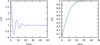Fig. 1 Evolution of the scale radius rc (left panel) and the logarithmic density slope (right panel).

2.2 Orbits integration

Equation (2) is integrated for each tracer particle using the quasi-symplectic method, introduced in Mannella (2004). For reasons of simplicity, but without loss of generality, we write it for the one-dimensional case as $$\begin{array}{cc}\hfill x^{\prime }=& x(t+\Delta t/2)=x(t)+\frac{\Delta t}{2}v(t)\hfill \\ \hfill v(t+\Delta t)=& c_2\left[c_{1}v(t)+\Delta t\nabla \Phi (x^{\prime })+d_1\widetilde{\delta f}(x^{\prime })\right]\hfill \\ \hfill x(t+\Delta t)=& x^{\prime }+\frac{\Delta t}{2}v(t+\Delta t)\hfill \end{array}$$(15)

In the expressions above Δt is the fixed time step (as a rule, here we adopt Δt = 10^{− 3} t_dyn , with $t_{\text{dyn}}\equiv \sqrt{r_c^3/GM}$ the crossing time of the asymptotic system, i.e. corresponding to the density profile at $t\to \infty$); $$\widetilde{\delta f}$$ is the normalized stochastic force (i.e. a dimen-sionless random variable sampled from the adimensionalized Eq. (13)); and $$c_1=1-\frac{\eta \Delta t}{2};c_2=\frac{1}{1+\eta \Delta t/2};d_1=\sqrt{2\zeta \eta \Delta t},$$(16) where the effective energy ζ, in the case of a delta correlated noise, is fixed by the standard deviation of ℱ as $$\langle \delta f(x,t)\delta f(x,t^{\prime })\rangle =2\eta \zeta \delta (t-t^{\prime }).$$(17)

Since for the Holtsmark distribution (13) the standard deviation, as well as all the other higher moments, are singular, our numerical scheme uses instead $f_{\text{HM}}/\sqrt{8\log 2}$, where f_HM is the full width at half maximum of the truncated distribution. We note that, for vanishing η and ζ, Eqs. (15) yield back the standard second-order and symplectic Leapfrog method.

2.3 Lyapunov exponents

The largest Lyapunov exponent Λ_max is estimated in numerical simulations (see e.g. Benettin et al. 1976; Kantz & Schreiber 2004; Skokos 2009) propagating up to a large time t = LΔt as $${\Lambda }_{\max }(t)=\frac{1}{L\Delta t}{\displaystyle \sum _{k=1}^L\ln }\frac{\Vert W(k\Delta t)\Vert }{\Vert W_0\Vert },$$(18) where W is the tangent-space vector, which for a 3D N-body system is the 6N-dimensional vector $$W=(w_i,{\stackrel{.}{w}}_i,\dots ,w_N,{\stackrel{.}{w}}_N).$$(19)

In the definitions above, $(w_i,{\stackrel{.}{w}}_i)$ are the tangent sub-space coordinates of the i-th degree of freedom (particle), and ||…|| is the standard Euclidean norm, here applied in ℝ^6N to the normalized w_is and ${\stackrel{.}{w}}_i\hspace{0.17em}\text{s}$. The vector W in initialized to W₀ at time t = 0. Technically speaking, the Lyapunov exponents are rigorously defined only in the infinite-time limit. In practical numerical simulations, we evaluate their approximate discrete definition (Eq. (18)) through sufficiently long integrations until convergence is numerically established. In the numerical experiments discussed hereafter we fixed a tolerance of the 0.001% on the fluctuations of the time series.

In systems where the tangent dynamics is not known or computationally unpractical (see e.g. Di Cintio & Trani 2025 and the discussion therein) one typically substitutes for W the distance between the reference orbit and that starting from a slightly perturbed initial condition, given by $$\tilde{W}=(r_i-r_i^{\prime },{\stackrel{.}{r}}_i-{\stackrel{.}{r}}_i^{\prime },\dots ,r_N-r_N^{\prime },{\stackrel{.}{r}}_N-{\stackrel{.}{r}}_N^{\prime }),$$(20) where the primed quantities refer to the perturbed phase-space trajectory. Defining a numerical Lyapunov exponent for a N = 1 dynamics governed by Eq. (2) is problematic for two reasons (see Arnold et al. 1986; Laffargue et al. 2016; Breden et al. 2024). On the one hand, this is due to the absence of a well-defined tangent dynamics for the stochastic term; on the other hand, it is due to the dependence of a given trajectory on the specific choice of random variables in implementing the noise protocol.

Here, we propose a simple empirical scheme¹ to estimate a proxy of the Lyapunov exponent of a particle orbit in a potential subjected to noise and friction, using multiple realizations of the perturbed trajectories appearing in the definition (20). For each tracer particle’s initial condition X_i we propagated N_e trajectories using different chains of pseudo-random numbers to sample the stochastic term, and another N_e trajectories starting from slightly perturbed initial condition X_i + ||ϵ|| with fixed ϵ and independent chains of pseudo-random numbers, as sketched in the left panel of Fig. 2. By doing so, we could therefore evaluate a set of N_e putative values of the largest Lyapunov exponent λ_* whose root mean square defines the value of the largest Lyapunov exponent of the wanted orbit defined by Eq. (2) as $${\lambda }_M^2=\frac{1}{N_e}{\displaystyle \sum _{i=1}^{N_e}{({\lambda }_{*,i}-{\overline{\lambda }}_{*})}^2},$$(21) where ${\overline{\lambda }}_{*}$ is the mean value of λ_*,i. In this work, as a rule, we used N_e = 20 and ϵ = 10⁻⁶.

Our model considers effectively a dissipationless scenario, with semi-analytical noise-friction processes introduced to mimic discreteness effects inherent in N-body systems. Hence, our total sum of Lyapunov exponents indeed remains close to zero by construction. A slight physical or numerical dissipation, would theoretically make this sum negative, and would thus influence longer-run dynamics. This is only evident in prohibitively long numerical integrations, often exceeding the timescale of the physical process of interest.

In order to verify that in the absence of noise the procedure introduced above gives an acceptable estimate of the largest Lyapunov exponent, we applied it to a simple chaotic model for which the variational equations necessary to integrate the tangent dynamics are simple and the largest Lyapunov exponent Λ_max was accurately estimated (Wolf et al. 1985). We considered the paradigmatic Lorenz (1963) system, defined by the set of three first-order ODEs $$\begin{array}{l}\dot{x}=\varsigma (y-x),\\ \dot{y}=x(\varrho -z)-y,\\ \dot{z}=xy-\beta z.\end{array}$$(22)

For the specific choice of model parameters ς = 10, ϱ = 28, and β = 8/3, it is known that Λ_max ≈ 0.906. In the right panel of Fig. 2, as an example, we show the convergence of the numerical estimation of the largest Lyapunov using an integration of the variational (tangent) dynamics, a single perturbed trajectory, and an ensemble average over ten nearby initial conditions. Remarkably, the value of Λ_max, marked in the figure by the horizontal dashed line is rather well approached in all cases.

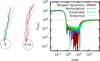Fig. 2 Left: sketch of the trajectory ensembles for the computation of the mean maximal Lyapunov exponent. Right: convergence of the maximal Lyapunov exponent Λmax for the Lorenz system.

2.4 Emittance and dynamical entropy

Defining a dynamical entropy for a system of independent particles with dynamics governed by Eq. (2) is rather subtle, due to the fact that for the particular case study of the present work the disorder and relaxation are induced by an external potential and stochastic process mimicking a real collective N-dynamics. Here, following Di Cintio & Casetti (2020b) (see also Kandrup et al. 2005 and references therein), we have evaluated the temporal evolution of the emittance, a quantity introduced in the context of charged particles beams (see e.g. Reiser 1991) and defined by $$\epsilon ={({\epsilon }_x{\epsilon }_y{\epsilon }_z)}^{1/3},{\epsilon }_i=\sqrt{\langle r_i^2\rangle \langle v_i^2\rangle -{\langle r_i{v}_i\rangle }^2},$$(23)

Where ⟨·⟩ denotes the ensemble averages. In the dynamics of a charged particle beam in an accelerator, the emittance quantifies the degree to which the individual particles depart from an idealized beam without space-charge effect, which means that a small emittance implies that particles are tightly packed in phasespace. Conversely, increasingly larger values of ε indicate that particles are more spread out over the accessible phase-space.

We recall that the definition (23) may be also thought of as the determinant of the variance-covariance matrix of the beam’s phase-space coordinates as $$\epsilon =\sqrt{\left|\begin{array}{cc}\langle x\cdot x\rangle & \langle x\cdot x^{\prime }\rangle \\ \langle x\cdot x^{\prime }\rangle & \langle x^{\prime }\cdot x^{\prime }\rangle \end{array}\right|},$$(24) from which it becomes evident that ε quantifies an effective (hyper-)surface enclosing the effective phase-space (hyper-) volume occupied by the system, in terms of its second-order statistics.

We note that Beraldo e Silva et al. (2019a,b) investigated the role of discreteness effects in effective N-body models using the discrete formulation of the Henon, Lynden-Bell & Tremaine entropy (hereafter HLBT; see Tremaine et al. 1986) defined for a particle-based model as $$\widehat{S}=\frac{1}{N}{\displaystyle \sum _{i=1}^N\ln }{D}_i^6+\ln \left[\frac{{\pi }^3}{6}(N-1)\right]+{\gamma }_{\text{EM}},$$(25) where $$D_i=\sqrt{{(r_i-r_{n,i})}^2+{(v_i-v_{n,i})}^2}$$(26) and γ_EM ≈ 0.57722 is the Euler-Mascheroni constant. In the definition above, r_n,i and v_n,i are the instantaneous position and velocity of the nearest phase-space neighbour of particle i (Leonenko et al. 2008). In a self-consistent N-body simulation of a VR process, Ŝ is expected to evolve towards a nearly invariant value. However, the same is also true for N independent particles starting from particular initial conditions and evolved in either regular or chaotic, static potentials, as shown in Beraldo e Silva et al. (2019b). The same is also true for the claimed N^1/6 scaling of the relaxation timescale associated with the growth of Ŝ for increasingly larger ensembles of tracer trajectories integrated in the same fixed external potential. This stems from the definition of D_i in Eq. (26) entering Eq. (25), that manifestly yields an average interparticle distance in ℝ⁶. The expression for the average interparticle distance for an ensemble of N particles in a volume V ∈ ℝ⁶ reads as $${\langle d\rangle }_{{ℝ}^6}=\frac{\Gamma (\frac{1}{6})}{6^{5/6}\sqrt{\pi }}\sqrt[6]{\frac{V}{N-1}},$$(27) from which the timescale dependence ∝N^−1/6 found in Beraldo e Silva et al. (2019b) naturally arises. We note that our method potentially bears some limitations as it is based on the propagation of tracer particles. However, in our case, the dynamics of these tracers become implicitly correlated by the local discreteness effects parametrized by η and δf.

It is well known that the emittance as defined in Eq. (23) can also be thought of as an entropy indicator (see e.g. Kim & Littlejohn 1995; Struckmeier 1996). In particular, Di Cintio & Casetti (2020b) showed that ε is constant for self-consistent equilibrium N-body models, provided that N is sufficiently large, while it increases exponentially for initially localized ensembles of particles in both frozen and active N-body gravitational models. A similar exponential emittance growth has also been reported by Kandrup et al. (2005) for the simulations of relaxing charged particle beams where the time evolution of ε is rather well fit by $$\epsilon (t)=C\sqrt{\frac{t}{N}}\exp (t\langle \lambda \rangle ),$$(28) where C is a dimensional constant and ⟨λ⟩ is the ensemble averaged largest Lyapunov exponent. We note that another important definition of dynamical entropy associated with the (spectrum of) trajectories of the Lyapunov exponents is the Kolmogorov-Sinai (KS, Kolmogorov 1958, 1959; Sinai 1959) entropy 𝒮_KS (see also Lichtenberg & Lieberman 2013). Given a discretization of time and phase-space, S _KS quantifies the probability that a trajectory occupies a cell j at a time t_n+1, conditioned on its history up to t_n. Pesin (1977) proved that the KS entropy of an orbit is always upper bounded by the sum of its positive Lyapunov exponents $${\mathcal{S}}_{\text{KS}}^{+}={\displaystyle \sum _{{\lambda }_i>0}{\lambda }_i}.$$(29)

Di Cintio & Trani (2025) used ${\mathcal{S}}_{\text{KS}}^{+}$ in addition to the largest Lyapunov exponent as an indicator of chaos to investigate the effect of increasing relativistic perturbations in some configurations of the gravitational three-body problem, finding that $S_{\text{KS}}^{+}$ shows a different trend with the strength of such perturbations than does Λ_max. In this work, however, a clear definition of the Lyapunov spectrum is not available because we are dealing with particle dynamics with stochastic terms, so we therefore resort to the numerical evaluation of dynamical entropies not involving the other λs.

3 Numerical experiments and results

3.1 Structural properties of the cold collapse

We integrated a wide set of orbits in time-dependent potentials with N-dependent noise and friction coefficients, simulating spherical dissipationless collapses.

In the simulations discussed here, we restrict ourselves to the cases where the initial conditions of N_t = 10⁴ tracer particles are characterized by zero velocity, and sample uniformly the density profile² corresponding to the embedding potential at t = 0. By doing so, we are considering a purely cold gravitational collapse (i.e. total initial kinetic energy K₀ = 0), which is the typical set up for N-body simulations to undergo a VR process (van Albada 1982; Londrillo et al. 1991; Trenti et al. 2005). As a rule, all simulations are extended up to 300t_dyn, so that the fluctuations of the numerically evaluated Lyapunov indicators fall within the requested tolerance window. In Fig. 3, we show the radial phasespace sections of N_t = 10⁴ tracer particles (i.e. radial coordinate r against radial velocity V_r) at times 0, 3, 10, 30, 100, and 300 in units of t_dyn in a self-similar collapse of a γ = 1 model without noise and friction (i.e. continuum limit). In this specific case the virial oscillation frequency is ω = 0.85, the damping time is τ_d = 13t_dyn, and the initial and final scale radii is r_c = 3 and 1, respectively. Remarkably, the distribution of points appears to be strikingly similar to that observed in self-consistent collapse simulations (see analogous plots in Londrillo et al. 1991; Nipoti et al. 2007; Di Cintio et al. 2013). The point colour-coding marks the radial³ positions at t = 0 revealing that, even in the absence of discreteness effects, a rapidly varying potential is enough to induce mixing and hence energy relaxation. In Fig. 4 we show the same distribution of phase-space coordinates for the case where the parent potential is perturbed by discreteness effects via friction and noise, corresponding to a N = 10⁴ N-body system. In this case, already at t = 10, we detect a more efficient mixing, represented by a stronger dispersion of points of the same colour, due to the action of the effective granularity. This is particularly evident in the final state at t = 300, which appears structurally similar to its parent continuum limit shown in Fig. 3, but with individual tracer particle phase-space positions almost entirely decorrelated from their state at t = 0.

In Fig. 5, we show as a function of N (represented by the increasingly lighter shades of blue) the final radial density distribution at t = 300 of the N_t tracers for the case of a γ = 1 self-similar collapse with r_c starting from 3 (magenta dashed line) and relaxing to 1 (black dashed line) with damped oscillations. With the notable exception of the discreteness effects-dominated N = 10⁴ case (corresponding to the dark blue line bearing an evident core-halo structure), all density profiles approach that of the asymptotic relaxed system, with some discrepancies related to the fixed number of tracer particles that, as a rule, we fixed to 10⁴. When the evolution of the external potential is characterized by values of ω⁻¹ and τ_c much larger than a typical crossing time (i.e. the evolution is adiabatic), the final density profile of the tracer distribution is expected to match to a higher degree that of the supporting external potential, as happens in the adiabatic squeezing techniques used to generate approximate equilibrium triaxial models starting from spherical N-body realizations with ergodic distribution functions (see Holley-Bockelmann et al. 2001).

Another quantity used to probe the mixing properties of phase-space is the differential energy distribution n(E) defined from the phase-space distribution function f (see e.g. Binney & Tremaine 2008; Baes & Dejonghe 2021) as $$n(E)={\displaystyle {\iint }_{\Pi }f}(r,v)\delta \left[E+v^2/2-\Phi (r)\right]\text{d}rdv,$$(30) where δ is the usual Dirac delta and Π is the phase-space volume occupied by the system. Figure 6 shows the evolution of n(E) in the self-similar collapse for the N = 10⁴, 10⁹, 10¹², and the continuum limit. Consistently with the density profile ρ, tracer particles in models with larger values of N do evolve towards nearly indistinguishable energy distributions, dictated by the VR. The lowest N = 10⁴ case, where the discreteness effects parametrized by η and ℱ are the largest, stands out for showing a markedly bimodal n(E). Interestingly, a similar form of the differential energy distribution has also been reported for N-body experiments of dissipationless collapses (see e.g. Di Cintio et al. 2013) for the cases with larger initial virial ratios (typically around 0.4–0.5), generally associated with a core-halo relaxed density distribution ρ. Remarkably, even though the simulations performed in this work were initialized with zero initial temperature, the larger the discreteness effects, the closer the dynamics of tracer particles to those of a system collapsing with a higher initial virial ratio. Moreover, this is also coherent with what was found for N-body simulations as a function of their particle resolution at a fixed type of initial condition (see e.g. Di Cintio 2024).

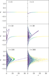Fig. 3 Radial phase-space section for an ensemble of tracers in a time-dependent potential simulation the self-similar collapse of a γ = 1 model in the continuum limit. The colour-coding indicates the initial radial position of each particle.

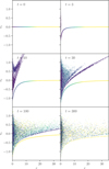Fig. 4 Same as in Fig. 3, but for a run including discreteness effects corresponding to a N = 104 system. Again, the colour-coding indicates the initial radial position of each particle.

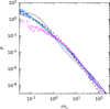Fig. 5 Density profile at t = 300 for the Nt = 104 tracers in models with effective N increasing from 104 to 1013, corresponding to increasingly lighter tones of blue (solid lines). Initial and final density profiles of the background model (purple and black dashed lines, respectively), and initial density profile of the tracers (points).

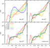Fig. 6 Evolution of the number energy distribution n(E) for N = 104, 109, 1012 and the continuum limit of a self-similar collapse.

3.2 Lyapunov exponents

It is well known that even in low dimensional models and for simple non-integrable potentials, the estimated values of the Lyapunov exponents might depend strongly on the orbital energy and even be different for initial conditions starting on the same energy surface but different phase-space coordinates. This is evident in Fig. 7 where we show for the same models of Fig. 6 the tracer particle largest Lyapunov exponent λ_M as a function of its orbital asymptotic energy E and (compare the colour-coding) its initial energy E₀. In general and consistently with the direct N-body calculations of Di Cintio & Casetti (2019) (see Fig. 10 therein), orbits that are localized in central regions and are therefore associated with lower energies show larger values of λ_M (i.e. are more chaotic) than those of weakly bound particles (i.e. E ≈ 0⁻). larger discreteness effects (i.e. lower N) induce a broader spread of λ_M at fixed final E, while also, as expected, triggering a more efficient energy mixing, possibly even after the VR phase than models governed by collective (external) potentials.

Individual values of the Lyapunov exponents are typically lower at given E for increasing values of N; however, moving in the direction of the continuum limit, those associated with weakly bound orbits have a stronger dependence with N, while between N = 10⁴ and 10⁹, where discreteness effects are still present but not dominant, the larger values of λ_M associated with orbits with E ≈ − 1 are substantially unchanged. This is also evident from the cumulative distribution C(λ_M) (i.e. ordered plot) over the whole ensemble of test particle orbits shown in Fig. 8 for system sizes N = 10⁴ (purple), 10⁹ (green), 10¹² (teal), and the continuum limit (orange) and, from left to right, a self-similar collapse of a γ = 1 model, a central cusp growth, and a collapse with steepening of the central cusp from γ₀ = 0 to γ_a = 1. In all cases we find that for N ≳ 10⁸ the normalized cumulative distribution of Lyapunov exponents converges to that of the continuum limit model below a critical value λ_M above which the distributions differ significantly as they have different slopes. Curiously, for intermediate and large N, C(λ_M) has several gaps that narrow in the continuum limit. We verified that this peculiar feature is not an artefact of the specific choice of initial conditions. The presence of these gaps, implies that the associated differential distribution of n(λ_M) has a gapped and multi-modal structure, as evidenced in Fig. 9 for the case of a self-similar collapse.

Following Di Cintio & Casetti (2019) in their analysis of equilibrium models, we computed λ_M for reference orbits starting from the same initial conditions at fixed initial energy E₀, evolving in models with different values of N. Figure 10 shows λ_M as a function of N for E₀ = −0.35 (diamonds), −0.1 (pentagons), −0.05 (triangles), and −0.01 (squares) in self-similar collapses with γ = 1 (left), cusp steepening (middle), and collapse with cusp steepening (right). Consistently with what is observed in Fig. 7, at fixed N larger (negative) initial energies reflect in more chaotic orbits, while particles initially less bound are typically associated with smaller values of their largest Lyapunov exponent. The latter scales with N for the considered values of E₀ with markedly different trends, though all are monotonically decreasing. Orbits starting with energies E₀ → 0⁻ yield (for large N values of finite time) Lyapunov exponents that are closer to their counterparts for the continuum model, where only the time-dependent collective potential mixes particle energies. The values of λ_M for this limit are indicated in figure by the horizontal dashed lines. We note that the Lyapunov indicators associated with particle energies of strongly bound orbits are far from their converged values in the continuum limit even for large and astrophysically relevant system sizes, which implies that orbits in the central regions of giant galaxies with N ≈ 10¹² ÷ 10¹³ stars might as well be wildly chaotic, even in the absence of significant deviations from spherical symmetry.

In order to quantify the dependence of the chaos indicator on the strength of the discreteness effects we have evaluated as a function of N the relevant moments of the distribution of largest Lyapunov exponents of the tracer orbits, namely the maximum λ_max, the median λ_50%, the mean λ_max, and the root mean square ⟨λ²⟩ ^1/2. In Fig. 11 these quantities are reported for the self-similar collapse (triangles), cusp steepening (circles), and collapse with cusp steepening (squares). In all cases the moments of n(λ_M) have broken power-law trends with N, nicely fit (compare the dashed lines in figure) by $$\lambda (N)=c\frac{\sqrt{N_{*}}}{N^{\alpha }{(N+N_{*})}^{\beta }},$$(31) where N_* is a scale system size and c a dimensional quantity ranging from 0.5 to ∼ 190. We observe that the trends of maximum λ_max and the root mean square ⟨λ²⟩ ^1/2 bear no significant difference along the three classes of numerical experiments, and the distribution of values at fixed N_* has little to no scattering. In the other two cases, the median and the mean, the trend for the collapses with cusp steepening is systematically intermediate between that for the self-similar collapse and the central cusp steepening. The values of α, β, and N_* are summarized in Table 1 below.

The scale size lies in the range 1.2 × 10⁷ ≲ N_* ≲ 8 × 10¹⁰, that implies for all the indicators the transition between a rather flat slope for low N and a N^1/6÷1/3 trend takes place at around N ≈ 10⁹. This could be interpreted as a predominance of microchaos below N_* , while at N > N_* the chaoticity of particle orbits is essentially due to the collective potential oscillations (coherent or incoherent) or possibly to the non-integrability of this potential itself for the case of static models (e.g. a triaxial system, not explored here).

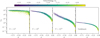Fig. 7 Largest Lyapunov exponent λM as a function of the final orbital energy for 104 particles propagating in effective self-similar collapsing γ = 1 system with N = 104, 107, 1012, and infinity. The colour-coding marks the initial value of particles specific energies E0.

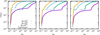Fig. 8 Cumulative distribution of the tracer orbits larger Lyapunov exponents for (from left to right) a self-similar collapse, a steepening of the inner density profile, and a collapse with strengthening of the central density cusp. The different sets of points mark the N = 104 (purple), N = 109 (green), N = 1012 (teal), and the continuum limit (orange).

3.3 Dynamical entropy

As we are dealing with a fixed number of tracer particles N_t < N, we modified the definition of the HLBT entropy Ŝ given in Eq. (25) by limiting the sum to N_t and substituting for (r_i − r_n,i)² and (v_i − v_n,i)² in D_i the quantities ${\overline{d}}_i^2$ and ${\sigma }_i^2$, respectively, defined as the square of the average interparticle distance and velocity dispersion of the underlying model at the position of the i-th tracer particle. The dynamical entropy S ^* adapted in this way (minus its initial value $S_0^{*}$) is plotted as a function of time in Fig. 12 for the systems discussed above (top panels) along with the corresponding tracer emittance (bottom panels).

In all cases, the modified HLBT entropy rapidly grows on a scale of about four time units, reaching a local maximum that is systematically larger for smaller N in the cases of collapsing models, and vice versa, that is smaller for the cusp steepening experiment. We observe that, for low N systems (indicated by darker shades of blue, green, and red), S ^* continues to grow even at later times after a damped oscillatory phase, with a multi power-law behaviour. By contrast, for increasingly larger values of N, the curve relaxes towards a nearly invariant value that is of the same order across all types of numerical experiments. This is consistent with the picture that in models with larger discreteness effects, particles initially lying on the same energy surface can explore a wider volume in phase-space, as the collective potential evolves towards a quasi-stationary state.

The emittance ε has a qualitatively similar trend to that of S ^*; however, the initial violent phases (e.g. below t ≈ 4) are indistinguishable for different values of N. We fitted the curve (see the black dashed lines in the figure Fig. 12) in this range with the generalization of Eq. (28) $$\epsilon (t)=C{(\frac{t}{N_{\text{t}}})}^a\exp (t\tilde{\lambda }).$$(32)

The fit parameters are summarized in Table 2. Curiously, in the collapse simulations the exponent a of the power-law envelope is close to 1/2, as one would expect from Eq. (28) recovered for example by Kandrup et al. (2004) for tracer particles propagating in frozen N-body potentials, while in the cusp growth case, the associated trend is almost linear (a ≈ 1.01). We find that the best-fit values of the inverse timescale λ are of the same order of magnitude of the average Lyapunov exponent evaluated for the continuum model (i.e. without noise and friction) over the time window where the first peak of ε happens. We performed additional runs with analogous initial conditions and different values of the tracer number N_t spanning from 3 × 10² to 2 × 10⁶, finding that both a and $\tilde{\lambda }$ are almost insensible to the number of tracers, provided that the latter is larger than ≈ 3 × 10³, while the final value attained by the emittance has systematically slightly lower values of N_t ≲ 3 × 10³ when N ≲ 10⁸ and it is almost independent of N_t for larger sizes, as shown in the lower panel of Fig. 13 for a collapse with cusp growth with N = 10¹¹. The HLBT entropy S ^* at fixed N (and in the continuum limit) is even less sensible to N_t, as shown in the top panel of Fig. 13, at variance with what is observed by Beraldo e Silva et al. (2019a,b) for ensembles of tracers propagated in static integrable or non-integrable potentials.

Comparing the evolution of S ^* and ε reveals that even though they both qualitatively behave as entropies (i.e. both are increasing functions of time), this seems to imply an almost negligible role of the discreteness effects during the initial VR phase, while S ^* has systematically a markedly N-dependent character for the whole simulation time span. This stems from the fact that the emittance is essentially a hypersurface enclosing the available phase-space volume, while the HLBT entropy S ^* is a local quantity, by construction dependent on the particle density and velocity distributions, thus intrinsically more sensible to N_t scaling and discreteness effects.

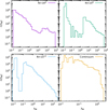Fig. 9 Distribution of maximal Lyapunov exponents for the tracer orbits in a self-similar collapse model, corresponding to the cumulative distribution of the left panel in Fig. 8.

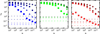Fig. 10 N-scaling of the mean maximal Lyapunov exponent for ensembles of tracers starting with different initial velocities, for the same experiments as in Fig. 11. The horizontal dashed lines mark the values attained for the continuum model without force fluctuations and friction.

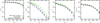Fig. 11 From left to right: an ensemble of tracers covering the whole accessible phase-space, N-scaling of the largest Lyapunov exponent λmax, median Lyapunov exponent λ50%, and mean value $\overline{\lambda }$, and root mean square of the distribution ⟨λ2⟩ 1/2. The blue triangles, green circles, and red square correspond to numerical experiments simulating a self-similar collapse, a steepening of the central density cusp (γ from 0 to 1), and a collapse with cusp steepening, respectively.

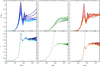Fig. 12 Modified HLBT entropy S * (top) and emittance ε growth (bottom) for (from left to right) self-similar collapse, cusp growth, and collapse with cusp growth. Increasingly lighter shades of blue, green, and red mark increasingly larger values of N. The dashed lines mark the best-fit growth trend of the exponential phase.

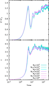Fig. 13 Modified HLBT entropy S * (top) and emittance ε growth (bottom) for a collapse with cusp growth with N = 1011 and different numbers of tracer particles in the range 103 ≤ Nt ≤ 106.

4 Outlook and discussion

We investigated the phase-space properties of orbit ensembles in time-dependent potentials simulating a process of VR including the N-dependent discreteness effects accounting for the granularity of gravitational systems. Using the stochastic integrator for independent trajectories developed by Pasquato & Di Cintio (2020) and Di Cintio et al. (2020) we investigated a self-similar collapse of a cuspy system, a cusp growth infall, and a collapse with cusp growth. Because our aim was to study the influence of micro-chaos induced by the finite-N nature in the case of large-N models, we analysed the energy-dependent phase-space spreading, the associated energy spectra, the distribution of the orbits’ largest Lyapunov exponents, and their mean values as a function of the system size N. In addition, we also studied the time evolution of two formulations of the dynamical entropy, as defined by Tremaine et al. (1986) and Reiser (1991).

We find that, for sufficiently accurate samplings of the initial phase-space, the distribution of tracers moving under the effect of a time-dependent relaxing potential and discreteness effects, here parametrized by friction and noise coefficients in the context of a Langevin stochastic model, asymptotically reproduce the energy and density distribution of the associated nearly invariant equilibrium state. The phase-space sections have a remarkably good agreement with those of full N-body simulations of dissipationless collapses with analogous initial conditions (see Fig. 3). We speculate that, by tuning the strength of the friction coefficient η and the fluctuation distribution ℱ in Eq. (2), one might improve the adiabatic squeezing scheme of Holley-Bockelmann et al. (2001) to produce flattened and triaxial models starting from a spherical seed system with ergodic distribution, as in the presence of discreteness effects the phase-space transport would be more efficient.

As expected, the values of the Lyapunov exponents for fixed initial orbital energy E₀ are systematically lower for increasing N at fixed simulation set-up, in agreement with the results by Di Cintio & Casetti (2019); Di Cintio et al. (2020) for direct N-body integrations of equilibrium models. As our method allows, at least in a statistical sense, large values of N to be probed in the astrophysically relevant range, we observed that there is a system size N_* ≈ 10⁹ for which the trends with N of some specific moments of the largest Lyapunov exponent distributions have a significant change of slope, seemingly independent of the number of tracer orbits N_t and the specific type of numerical experiment. We interpret this fact as the existence of a regime of system sizes below which the chaos induced by discreteness effects dominates the one associated with collective oscillations during the phase-mixing process after the initial phase of the collapse, and possibly at the origin of what is commonly referred to as ‘incomplete violent relaxation’ in numerical experiments (see Trenti & Bertin 2004, 2005; Trenti et al. 2005). This is also in agreement with the evolution of the dynamical entropies (see Fig. 12). In particular, the tracer ensemble emittance ε has the same behaviour during the first violent phase, for all N and for all N_t at fixed N, while it shows a rather clear N-dependence during the virial oscillation phases at later times with a distinct drift for the lower N cases. This is in apparent contradiction with the argument of Beraldo e Silva et al. (2017) that a description in terms of the CBE of the VR is erroneous as it would imply a constant dynamical entropy even during violent relaxation. We conjecture that the timescale of VR in some cases might be shorter than the smallest Lyapunov timescale (i.e. the largest Lyapunov exponent) of the full N-body problem, but at the same time longer than the Lyapunov timescales of individual particle orbits. This implies that a given model could be relatively insensible to the discreteness effects during the fast VR phase, even though the distribution of orbits of the Lyapunov exponents has a larger variance and mean for decreasing N (see Figs. 11 and 12). The origin of this and other discrepancies are essentially to be attributed to the different indicators employed to measure chaos and relaxation. Local indicators (i.e. individual orbit Lyapunov exponents and their distributions) do keep track of micro-chaos, while integrated quantities such as the HLBT entropy are more sensitive to collective processes.

More broadly, this point likely connects to the argument by Arad & Lynden-Bell (2005) that violent relaxation is largely insensitive to the fine-grained evolution of f in phase space, even within the collisionless CBE picture. As a result, any instance of violent relaxation is inherently incomplete. The subsequent, more gradual fluctuations that steer the system towards a quasi-equilibrium state must therefore be understood only in a coarse-grained sense, involving a discretized phase-space density $\overline{f}$, as in Chavanis (1998) and Barbieri et al. (2022).

Acknowledgements

We thank the anonymous referee for insightful suggestions that improved the manuscript. P.F.D.C. wishes to acknowledge funding by “Fondazione Cassa di Risparmio di Firenze” under the project HIPERCRHEL for the use of high performance computing resources at the University of Firenze. A.A.T. acknowledges support from the Horizon Europe research and innovation programs under the Marie Skłodowska-Curie grant agreement no. 101103134.

References

All Tables

All Figures

	Fig. 1 Evolution of the scale radius rc (left panel) and the logarithmic density slope (right panel).
In the text

	Fig. 2 Left: sketch of the trajectory ensembles for the computation of the mean maximal Lyapunov exponent. Right: convergence of the maximal Lyapunov exponent Λmax for the Lorenz system.
In the text

	Fig. 3 Radial phase-space section for an ensemble of tracers in a time-dependent potential simulation the self-similar collapse of a γ = 1 model in the continuum limit. The colour-coding indicates the initial radial position of each particle.
In the text

	Fig. 4 Same as in Fig. 3, but for a run including discreteness effects corresponding to a N = 104 system. Again, the colour-coding indicates the initial radial position of each particle.
In the text

	Fig. 5 Density profile at t = 300 for the Nt = 104 tracers in models with effective N increasing from 104 to 1013, corresponding to increasingly lighter tones of blue (solid lines). Initial and final density profiles of the background model (purple and black dashed lines, respectively), and initial density profile of the tracers (points).
In the text

	Fig. 6 Evolution of the number energy distribution n(E) for N = 104, 109, 1012 and the continuum limit of a self-similar collapse.
In the text

	Fig. 7 Largest Lyapunov exponent λM as a function of the final orbital energy for 104 particles propagating in effective self-similar collapsing γ = 1 system with N = 104, 107, 1012, and infinity. The colour-coding marks the initial value of particles specific energies E0.
In the text

	Fig. 8 Cumulative distribution of the tracer orbits larger Lyapunov exponents for (from left to right) a self-similar collapse, a steepening of the inner density profile, and a collapse with strengthening of the central density cusp. The different sets of points mark the N = 104 (purple), N = 109 (green), N = 1012 (teal), and the continuum limit (orange).
In the text

	Fig. 9 Distribution of maximal Lyapunov exponents for the tracer orbits in a self-similar collapse model, corresponding to the cumulative distribution of the left panel in Fig. 8.
In the text

	Fig. 10 N-scaling of the mean maximal Lyapunov exponent for ensembles of tracers starting with different initial velocities, for the same experiments as in Fig. 11. The horizontal dashed lines mark the values attained for the continuum model without force fluctuations and friction.
In the text

Fig. 11 From left to right: an ensemble of tracers covering the whole accessible phase-space, N-scaling of the largest Lyapunov exponent λmax, median Lyapunov exponent λ50%, and mean value $\overline{\lambda }$, and root mean square of the distribution ⟨λ2⟩ 1/2. The blue triangles, green circles, and red square correspond to numerical experiments simulating a self-similar collapse, a steepening of the central density cusp (γ from 0 to 1), and a collapse with cusp steepening, respectively.

In the text

	Fig. 12 Modified HLBT entropy S * (top) and emittance ε growth (bottom) for (from left to right) self-similar collapse, cusp growth, and collapse with cusp growth. Increasingly lighter shades of blue, green, and red mark increasingly larger values of N. The dashed lines mark the best-fit growth trend of the exponential phase.
In the text

	Fig. 13 Modified HLBT entropy S * (top) and emittance ε growth (bottom) for a collapse with cusp growth with N = 1011 and different numbers of tracer particles in the range 103 ≤ Nt ≤ 106.
In the text

References

- Arad, I., & Lynden-Bell, D. 2005, MNRAS, 361, 385 [Google Scholar]
- Arnold, L., Kliemann, W., & Oeljeklaus, E. 1986, in Lyapunov Exponents, eds. L. Arnold, & V. Wihstutz (Berlin, Heidelberg: Springer Berlin Heidelberg), 85 [Google Scholar]
- Baes, M., & Dejonghe, H. 2021, A&A, 653, A140 [NASA ADS] [CrossRef] [EDP Sciences] [Google Scholar]
- Banik, U., Weinberg, M. D., & van den Bosch, F. C. 2022, ApJ, 935, 135 [NASA ADS] [CrossRef] [Google Scholar]
- Barbieri, L., Di Cintio, P., Giachetti, G., Simon-Petit, A., & Casetti, L. 2022, MNRAS, 512, 3015 [Google Scholar]
- Benettin, G., Galgani, L., & Strelcyn, J.-M. 1976, Phys. Rev. A, 14, 2338 [Google Scholar]
- Beraldo e Silva, L., de Siqueira Pedra, W., Sodré, L., Perico, E. L. D., & Lima, M. 2017, ApJ, 846, 125 [Google Scholar]
- Beraldo e Silva, L., de Siqueira Pedra, W., & Valluri, M. 2019a, ApJ, 872, 20 [Google Scholar]
- Beraldo e Silva, L., de Siqueira Pedra, W., Valluri, M., Sodré, L., & Bru, J.-B. 2019b, ApJ, 870, 128 [Google Scholar]
- Beraldo e Silva, L., Valluri, M., Vasiliev, E., et al. 2024, arXiv e-prints [arXiv:2407.07947] [Google Scholar]
- Binney, J., & Tremaine, S. 2008, Galactic Dynamics 2nd edn. (Princeton, NJ, USA: Princeton University Press) [Google Scholar]
- Breden, M., Chu, H., Lamb, J. S. W., & Rasmussen, M. 2024, arXiv e-prints [arXiv:2411.07064] [Google Scholar]
- Campa, A., Dauxois, T., Fanelli, D., & Ruffo, S. 2014, Physics of long-range interacting systems (Oxford: Oxford University Press) [Google Scholar]
- Casetti, L., Pettini, M., & Cohen, E. G. D. 2000, Phys. Rep., 337, 237 [Google Scholar]
- Cerruti-Sola, M., & Pettini, M. 1995, Phys. Rev. E, 51, 53 [Google Scholar]
- Chandrasekhar, S. 1943, ApJ, 97, 255 [Google Scholar]
- Chandrasekhar, S., & von Neumann, J. 1943, ApJ, 97, 1 [NASA ADS] [CrossRef] [Google Scholar]
- Chavanis, P.-H. 1998, MNRAS, 300, 981 [Google Scholar]
- Ciotti, L. 2010, in American Institute of Physics Conference Series, 1242, Plasmas in the Laboratory and the Universe: Interactions, Patterns, and Turbulence, eds. G. Bertin, F. de Luca, G. Lodato, R. Pozzoli, & M. Romé (AIP), 117 [Google Scholar]
- Dehnen, W. 1993, MNRAS, 265, 250 [NASA ADS] [CrossRef] [Google Scholar]
- Dehnen, W. 2005, MNRAS, 360, 892 [Google Scholar]
- Di Cintio, P. 2024, A&A, 683, A254 [NASA ADS] [CrossRef] [EDP Sciences] [Google Scholar]
- Di Cintio, P., & Casetti, L. 2019, MNRAS, 489, 5876 [NASA ADS] [CrossRef] [Google Scholar]
- Di Cintio, P., & Casetti, L. 2020a, MNRAS, 494, 1027 [NASA ADS] [CrossRef] [Google Scholar]
- Di Cintio, P., & Casetti, L. 2020b, Proc. Int. Astron. Union, 14, 426 [Google Scholar]
- Di Cintio, P., & Trani, A. A. 2025, A&A, 693, A53 [NASA ADS] [CrossRef] [EDP Sciences] [Google Scholar]
- Di Cintio, P., Ciotti, L., & Nipoti, C. 2013, MNRAS, 431, 3177 [NASA ADS] [CrossRef] [Google Scholar]
- Di Cintio, P., Ciotti, L., & Nipoti, C. 2020, Proc. Int. Astron. Union, 14, 93 [Google Scholar]
- El-Zant, A. A. 2002, MNRAS, 331, 23 [CrossRef] [Google Scholar]
- El-Zant, A. A., Everitt, M. J., & Kassem, S. M. 2019, MNRAS, 484, 1456 [NASA ADS] [CrossRef] [Google Scholar]
- Goodman, J., Heggie, D. C., & Hut, P. 1993, ApJ, 415, 715 [Google Scholar]
- Gurzadian, V. G., & Savvidy, G. K. 1986, A&A, 160, 203 [NASA ADS] [Google Scholar]
- Gurzadyan, V. G., & Kocharyan, A. A. 2009, A&A, 505, 625 [NASA ADS] [CrossRef] [EDP Sciences] [Google Scholar]
- He, P. 2013, Int. J. Mod. Phys. B, 27, 1361011 [Google Scholar]
- Hemsendorf, M., & Merritt, D. 2002, ApJ, 580, 606 [NASA ADS] [CrossRef] [Google Scholar]
- Holley-Bockelmann, K., Mihos, J. C., Sigurdsson, S., & Hernquist, L. 2001, ApJ, 549, 862 [Google Scholar]
- Holtsmark, J. 1919, Ann. Phys., 363, 577 [Google Scholar]
- Kandrup, H. E. 1987, MNRAS, 225, 995 [Google Scholar]
- Kandrup, H. E. 1996, in Proceedings of the Seventh Marcel Grossman Meeting on Recent Developments in Theoretical and Experimental General Relativity, Gravitation, and Relativistic Field Theories, 7, eds. R. T. Jantzen, G. Mac Keiser, & R. Ruffini, 167 [Google Scholar]
- Kandrup, H. E. 1998a, Ann. N. Y. Acad. Sci., 848, 28 [Google Scholar]
- Kandrup, H. E. 1998b, ApJ, 500, 120 [Google Scholar]
- Kandrup, H. E., & Novotny, S. J. 2004, Celest. Mech. Dyn. Astron., 88, 1 [Google Scholar]
- Kandrup, H. E., & Sideris, I. V. 2001, Phys. Rev. E, 64, 056209 [NASA ADS] [CrossRef] [Google Scholar]
- Kandrup, H. E., & Sideris, I. V. 2003, ApJ, 585, 244 [Google Scholar]
- Kandrup, H. E., Vass, I. M., & Sideris, I. V. 2003, MNRAS, 341, 927 [Google Scholar]
- Kandrup, H. E., Sideris, I. V., & Bohn, C. L. 2004, Phys. Rev. Acceler. Beams, 7, 014202 [Google Scholar]
- Kandrup, H. E., Bohn, C. L., Kishek, R. A., et al. 2005, Ann. N. Y. Acad. Sci., 1045, 12 [Google Scholar]
- Kang, D. B., & He, P. 2011, A&A, 526, A147 [NASA ADS] [CrossRef] [EDP Sciences] [Google Scholar]
- Kantz, H., & Schreiber, T. 2004, Nonlinear Time Series Analysis, Cambridge Nonlinear Science Series (Cambridge University Press) [Google Scholar]
- Kim, K.-J., & Littlejohn, R. 1995, in Proceedings Particle Accelerator Conference, 5, 3358 [Google Scholar]
- Kolmogorov, A. 1958, Dokl. Akad. Nauk SSSR, 119, 861 [Google Scholar]
- Kolmogorov, A. 1959, Dokl. Akad. Nauk SSSR, 124, 754 [Google Scholar]
- Laffargue, T., Tailleur, J., & van Wijland, F. 2016, J. Statist. Mech.: Theory Exp., 2016, 034001 [Google Scholar]
- Leonenko, N., Pronzato, L., & Savani, V. 2008, Ann. Statist., 36, 2153 [Google Scholar]
- Levin, Y., Pakter, R., Rizzato, F. B., Teles, T. N., & Benetti, F. P. C. 2014, Phys. Rep., 535, 1 [Google Scholar]
- Lichtenberg, A., & Lieberman, M. 2013, Regular and Chaotic Dynamics, Applied Mathematical Sciences (Springer New York) [Google Scholar]
- Londrillo, P., Messina, A., & Stiavelli, M. 1991, MNRAS, 250, 54 [NASA ADS] [Google Scholar]
- Lorenz, E. N. 1963, J. Atmos. Sci., 20, 130 [Google Scholar]
- Lynden-Bell, D. 1967, Mon. Not. Roy. Astron. Soc., 136, 101 [Google Scholar]
- Madsen, J. 1987, ApJ, 316, 497 [Google Scholar]
- Mannella, R. 2004, Phys. Rev. E, 69 [Google Scholar]
- Merritt, D. 2005, Ann. N. Y. Acad. Sci., 1045, 3 [Google Scholar]
- Miller, R. H. 1964, ApJ, 140, 250 [NASA ADS] [CrossRef] [Google Scholar]
- Miller, R. H. 1971, J. Computat. Phys., 8, 449 [Google Scholar]
- Nakamura, T. K. 2000, ApJ, 531, 739 [Google Scholar]
- Nipoti, C., Londrillo, P., & Ciotti, L. 2007, ApJ, 660, 256 [NASA ADS] [CrossRef] [Google Scholar]
- Padmanabhan, T. 1990, Phys. Rep., 188, 285 [Google Scholar]
- Pasquato, M., & Di Cintio, P. 2020, A&A, 640, A79 [NASA ADS] [CrossRef] [EDP Sciences] [Google Scholar]
- Pesin, Y. B. 1977, Russ. Math. Surv., 32, 55 [Google Scholar]
- Reiser, M. 1991, J. Appl. Phys., 70, 1919 [Google Scholar]
- Severne, G., & Luwel, M. 1980, Ap&SS, 72, 293 [Google Scholar]
- Sideris, I. V., & Kandrup, H. E. 2002, Phys. Rev. E, 65 [Google Scholar]
- Sideris, I. V., & Kandrup, H. E. 2004, ApJ, 602, 678 [Google Scholar]
- Sinai, Y. 1959, Dokl. Akad. Nauk SSSR, 124, 768 [Google Scholar]
- Skokos, C. 2009, The Lyapunov Characteristic Exponents and Their Computation (Springer Berlin Heidelberg), 63 [Google Scholar]
- Soker, N. 1996, ApJ, 457, 287 [Google Scholar]
- Struckmeier, J. 1996, Phys. Rev. E, 54, 830 [Google Scholar]
- Sylos Labini, F. 2012, MNRAS, 423, 1610 [Google Scholar]
- Tremaine, S., Henon, M., & Lynden-Bell, D. 1986, MNRAS, 219, 285 [NASA ADS] [CrossRef] [Google Scholar]
- Tremaine, S., Richstone, D. O., Byun, Y.-I., et al. 1994, AJ, 107, 634 [CrossRef] [Google Scholar]
- Trenti, M., & Bertin, G. 2004, arXiv e-prints [arXiv:astro-ph/0406236] [Google Scholar]
- Trenti, M., & Bertin, G. 2005, A&A, 429, 161 [NASA ADS] [CrossRef] [EDP Sciences] [Google Scholar]
- Trenti, M., Bertin, G., & van Albada, T. S. 2005, A&A, 433, 57 [NASA ADS] [CrossRef] [EDP Sciences] [Google Scholar]
- van Albada, T. S. 1982, MNRAS, 201, 939 [NASA ADS] [CrossRef] [Google Scholar]
- Vass, I. M., Kandrup, H. E., & Terzić, B. 2003, in American Astronomical Society Meeting Abstracts, 203, 91.11 [Google Scholar]
- Vesperini, E. 1992, A&A, 266, 215 [Google Scholar]
- Wolf, A., Swift, J. B., Swinney, H. L., & Vastano, J. A. 1985, Physica D Nonlinear Phenomena, 16, 285 [NASA ADS] [CrossRef] [Google Scholar]
- Worrakitpoonpon, T. 2024, Phys. Rev. E, 109, 054118 [Google Scholar]
We recall that Kandrup & Sideris (2003) also presented a scheme to evaluate λM for models with a stochastic component, based on averages over orbit segments.
The density of tracer particles divided by the effective ρ of the background system is constant over all radii.
Since in this particular numerical experiment the initial kinetic energies were set to 0, the total particle initial energy (i.e. potential only) is directly proportional to the initial radial position.