| Issue |
A&A
Volume 693, January 2025
|
|
|---|---|---|
| Article Number | A53 | |
| Number of page(s) | 9 | |
| Section | Celestial mechanics and astrometry | |
| DOI | https://doi.org/10.1051/0004-6361/202452678 | |
| Published online | 03 January 2025 | |
Partial suppression of chaos in relativistic three-body problems
1
National Council of Research – Institute of Complex Systems,
Via Madonna del piano 10,
50019
Sesto Fiorentino,
Italy
2
National Institute of Nuclear Physics (INFN) – Florence unit,
via G. Sansone 1,
50019
Sesto Fiorentino,
Italy
3
National Institute of Astrophysics – Arcetri Astrophysical Observatory (INAF-OAA),
Piazzale E. Fermi 5,
50125
Firenze,
Italy
4
Niels Bohr International Academy, Niels Bohr Institute,
Blegdamsvej 17,
2100
Copenhagen,
Denmark
★ Corresponding authors; This email address is being protected from spambots. You need JavaScript enabled to view it.
, This email address is being protected from spambots. You need JavaScript enabled to view it.
Received:
20
October
2024
Accepted:
27
November
2024
Abstract
Context. Recent numerical results seem to suggest that, in certain regimes of typical particle velocities, when the post-Newtonian (PN) force terms are included, the gravitational N-body problem (for 3 ≤ N ≲ 103) is intrinsically less chaotic than its classical counterpart, which exhibits a slightly larger maximal Lyapunov exponent Λmax.
Aims. In this work, we explore the dynamics of wildly chaotic, regular and nearly regular configurations of the three-body problem with and without the PN corrective terms, with the aim being to shed light on the behaviour of the Lyapunov spectra under the effect of the PN corrections.
Methods. Because the interaction of the tangent-space dynamics in gravitating systems – which is needed to evaluate the Lyapunov exponents – becomes rapidly computationally heavy due to the complexity of the higher-order force derivatives involving multiple powers of v/c, we introduce a technique to compute a proxy of the Lyapunov spectrum based on the time-dependent diagonalization of the inertia tensor of a cluster of trajectories in phase-space. In addition, we also compare the dynamical entropy of the classical and relativistic cases.
Results. We find that, for a broad range of orbital configurations, the relativistic three-body problem has a smaller Λmax than its classical counterpart starting with the exact same initial conditions. However, the other (positive) Lyapunov exponents can be either lower or larger than the corresponding classical ones, thus suggesting that the relativistic precession effectively reduces chaos only along one (or a few) directions in phase-space. As a general trend, the dynamical entropy of the relativistic simulations as a function of the rescaled speed of light falls below the classical value over a broad range of values.
Conclusions. We observe that analyses based solely on Λmax could lead to misleading conclusions regarding the chaoticity of systems with small (and possibly large) N.
Key words: chaos / relativistic processes / methods: numerical / celestial mechanics
© The Authors 2025
 Open Access article, published by EDP Sciences, under the terms of the Creative Commons Attribution License (https://creativecommons.org/licenses/by/4.0), which permits unrestricted use, distribution, and reproduction in any medium, provided the original work is properly cited.
This article is published in open access under the Subscribe to Open model. This email address is being protected from spambots. You need JavaScript enabled to view it. to support open access publication.
1 Introduction
The gravitational N-body problem (for N ≥ 3) is intrinsically chaotic due to the large number of degrees of freedom with respect to its conserved quantities (Contopoulos 2002). Since the seminal work of Miller (1964, 1971), much attention has been paid to the scaling of the degree of this chaoticity, which is quantified in terms of the maximal Lyapunov exponent Λmax (e.g. see Lichtenberg & Lieberman 1992) for a total number of particles N. In numerical simulations, Λmax is usually estimated using the standard Benettin et al. (1976) method, as
 (1)
(1)
for a (large) time t = LΔt, where W is the 6N-dimensional tangent-space vector,
 (2)
(2)
which is initialised to W0 at time t = 0, and ||…|| is the standard Euclidean norm, here applied in ℝ6N to adimensionalized wis and Wis. For classical gravitational N-body dynamics of particles of equal mass m,
 (3)
(3)
the variational equations in tangent space needed to evaluate W6N are (see also Rein & Tamayo 2016)
![Mathematical equation: ${\mathop {\bf{w}}\limits^{..} _i} = - Gm\sum\limits_{i \ne j = 1}^N {\left[ {{{{{\bf{w}}_i} - {{\bf{w}}_j}} \over {r_{ij}^3}} - 3\left( {{{\bf{r}}_i} - {{\bf{r}}_j}} \right){{\left\langle {\left( {{{\bf{w}}_i} - {{\bf{w}}_j}} \right)\left( {{{\bf{r}}_i} - {{\bf{r}}_j}} \right)} \right\rangle } \over {r_{ij}^5}}} \right]} ,$](/articles/aa/full_html/2025/01/aa52678-24/aa52678-24-eq4.png) (4)
(4)
where G is the usual gravitational constant, rij = ||ri −rj|| , and ⟨xy⟩ indicates the scalar product.
In the continuum limit (N → ∞) assumption, which is formulated in terms of one-particle phase-space distribution functions f by the collisionless Boltzmann equation (e.g. see Binney & Tremaine 2008), no chaos should be present in the sense of asymptotically diverging initially nearby trajectories (Kandrup & Smith 1991). For this reason, for a given form of the initial density and velocity profiles, Λmax − evaluated in simulations via Eq. (1) – is expected to decrease for increasing N at fixed total mass M = mN.
Using semi-analytical arguments, Gurzadyan & Savvidy (1986); Gurzadyan & Kocharyan (2009); Ovod & Ossipkov (2013) estimated that
 (5)
(5)
Since then, several numerical studies (Goodman et al. 1993; Habib et al. 1997; Kandrup & Sideris 2001; Sideris & Kandrup 2002; Hemsendorf & Merritt 2002; Cipriani & Pettini 2003; El-Zant 2002; Kandrup & Siopis 2003; El-Zant et al. 2019, and references therein) based on both single-particle integration in fixed N-body potentials and the full solution of the N -body problem seem to indicate that individual orbits become more regular (i.e. approach their counterparts propagated in the smooth mean field gravitational potential) as N increases. On the other hand, their largest Lyapunov exponents remain somewhat independent of N, while the full N-particle dynamics become less chaotic as N increases with a N−1/2 trend, which is at odds with the Gurzadyan & Savvidy (1986) N−1/3 estimate1.
In a series of papers, Di Cintio & Casetti (2019, 2020a,b) performed extensive direct numerical integrations with 102 ≤ N ≤ 105 for a wide range of density profiles and velocity distribution. These authors found that Λmax(N) exhibits a strong dependence on the specific choice of the initial conditions, while being always bounded between the N−1/2 and N−1/3 trends. The N-scaling of the Lyapunov exponents of individual particle trajectories for a given model is strongly dependent on the initial energy and angular momentum of the particles, and the somewhat flat behaviour observed in previous studies was merely an effect of the low number of particles employed.
More recently, Portegies Zwart et al. (2022) repeated the numerical experiments of Di Cintio & Casetti (2019) for 3 ≤ N ≤ 105 using the arbitrary precision integrator BRUTUS (see Portegies Zwart & Boekholt 2014), and also including the relativistic correction to the interparticle forces at 1 /c2 order using the Einstein-Infeld-Hoffmann Lagrangian (EIH, Einstein et al. 1938) equations as well as the first post-Newtonian-order perturbative term (1PN, Blanchet 2024). One of the main results of the analysis presented by Portegies Zwart et al. (2022) is that, surprisingly, at typical velocities vtyp of approximately 2 × 10⁻³ or higher – in units of the speed of light c −, the 1PN relativistic N -body systems are less chaotic than their classical counterparts, exhibiting a smaller maximum Lyapunov exponent Λmax . Remarkably, Boekholt et al. (2021) found a similar trend in the context of the relativistic Pythagorean three-body problem (i.e. the three bodies of masses m1 = 3, m2 = 4, and m3 = 5 start at rest at the vertexes of a right-angled triangle to engage in complex dynamics involving multiple encounters before expelling the lightest body m1 ; see Burrau 1913) with PN corrections of up to the order 2.5. It is worth mentioning that similar studies, though not concentrating on Lyapunov exponents, have also been carried out by Valtonen et al. (1995) and Chitan et al. (2022), with the authors concluding that increasing the mass of the components favours the merger rather than the escape of m1 .
Kovács et al. (2011) investigated the Sitnikov (1960) three- body problem (i.e. the third body of mass m3 ≈ 0 moves along a straight line orthogonal to the plane of the main binary and crosses its centre of mass), and found that the inclusion of the 1PN term systematically reduces the central regular phasespace region for increasing values of the parameter α = G(m1 + m2)/ac2, where a is the semi-major axis of the binary of m1 and m2. Moreover, Dubeibe et al. (2017a,b) analysed the Poincaré sections2 and the Lyapunov spectra of the relativistic circular restricted three-body problem (see Maindl & Dvorak 1994). Their findings suggest that the so-called pseudo-Newtonian approximation with the Fodor-Hoenselaers-Perjés potentials (see Fodor et al. 1989, see also Steklain & Letelier 2006 and references therein) enhances chaoticity in classically regular orbits, while significantly reducing chaos in some irregular orbits for specific ranges of energy and Jacobi constant.
A clear interpretation of this intriguing finding (i.e. perturbing a chaotic system may either reduce or enhance its degree of chaos) is still missing. Of course, one might argue that, even if the initial conditions of the numerical experiments are the same, the classical and relativistic N -body problems are described by two different Hamiltonians, ℌclass and ℌrel , with potentially differently structured energy surfaces. A fair comparison of their maximal Lyapunov exponents is thus most an likely ill-posed problem, except in regimes of reasonably low values of vtyp/c such that one can assume, perturbatively, that ℌreļ = ℌcass + єH, where the small (i.e. є << 1) perturbation term єH contains the PN corrections.
Aiming to shed some light on the unclear behaviour described above, in this work we explore this matter further by estimating the positive part of the Lyapunov spectrum as well as the dynamical entropy of four representative, relativistic three-body problems and their parent classical systems.
The rest of the paper is structured as follows: In Sect. 2 we introduce the governing equations, discuss the numerical integration, and describe the procedure to evaluate the Lyapunov exponents. In Sect. 3 we present our numerical simulations and discuss the results. Finally, in Sect. 4 we draw our conclusions and interpret our findings within the context provided by previous work.
2 Methods
2.1 Numerical integration
At variance with Boekholt et al. (2021), we consider the relativistic corrections up to the 2PN order (i.e. we neglect the dissipative 2.5PN terms associated with the gravitational wave emission, Blanchet 1996 and higher corrections), where the Equations of motion in Eq.(3) are augmented by the extra terms P1 and P2 given (e.g. see Damour & Deruelle 1985; Soffel 1989; Spurzem et al. 2008) by
![Mathematical equation: $\eqalign{ & {{\bf{P}}_{1i}} = {G \over {{c^2}}}\sum\limits_{i \ne j = 1}^N {{{{m_j}} \over {r_{ij}^2}}} \left[ {\left( { - v_i^2 - 2v_j^2 + 4\left\langle {{{\bf{v}}_i}{{\bf{v}}_j}} \right\rangle + {3 \over 2}\left\langle {{{\bf{n}}_{ij}}{{\bf{v}}_j}} \right\rangle } \right.} \right. \cr & & \left. {\left. { + {{5G{m_i} + 4G{m_j}} \over {{r_{ij}}}}} \right){{\bf{n}}_{ij}} + \left( {{{\bf{v}}_i} - {{\bf{v}}_j}} \right)\left( {4\left\langle {{{\bf{n}}_{ij}}{{\bf{v}}_i}} \right\rangle - 3\left\langle {{{\bf{n}}_{ij}}{{\bf{v}}_j}} \right\rangle } \right)} \right] \cr} $](/articles/aa/full_html/2025/01/aa52678-24/aa52678-24-eq6.png) (6)
(6)
and
![Mathematical equation: $\eqalign{ & {{\bf{P}}_{2i}} = {G \over {{c^4}}}\sum\limits_{i \ne j = 1}^N {{{{m_j}} \over {r_{ij}^2}}} \left\{ {\left[ { - 2v_j^4 + 4v_j^2\left\langle {{{\bf{v}}_i}{{\bf{v}}_j}} \right\rangle - 2{{\left\langle {{{\bf{v}}_i}{{\bf{v}}_j}} \right\rangle }^2}} \right.} \right. \cr & & + {3 \over 2}v_i^2{\left\langle {{{\bf{n}}_{ij}}{{\bf{v}}_j}} \right\rangle ^2} + {9 \over 2}v_j^2{\left\langle {{{\bf{n}}_{ij}}{{\bf{v}}_j}} \right\rangle ^2} - 6\left\langle {{{\bf{v}}_i}{{\bf{v}}_j}} \right\rangle {\left\langle {{{\bf{n}}_{ij}}{{\bf{v}}_j}} \right\rangle ^2} - {{15} \over 8}{\left\langle {{{\bf{n}}_{ij}}{{\bf{v}}_j}} \right\rangle ^4} \cr & & + {{G{m_j}} \over {{r_{ij}}}}\left( {4v_j^2 - 8\left\langle {{{\bf{v}}_i}{{\bf{v}}_j}} \right\rangle + 2{{\left\langle {{{\bf{n}}_{ij}}{{\bf{v}}_i}} \right\rangle }^2} - 4\left\langle {{{\bf{n}}_{ij}}{{\bf{v}}_i}} \right\rangle \left\langle {{{\bf{n}}_{ij}}{{\bf{v}}_j}} \right\rangle - 6{{\left\langle {{{\bf{n}}_{ij}}{{\bf{v}}_j}} \right\rangle }^2}} \right) \cr & & \quad + {{G{m_i}} \over {{r_{ij}}}}\left( { - {{15} \over 4}v_i^2 + {5 \over 4}v_j^2 - {5 \over 2}\left\langle {{{\bf{v}}_i}{{\bf{v}}_j}} \right\rangle + {{39} \over 2}{{\left\langle {{{\bf{n}}_{ij}}{{\bf{v}}_i}} \right\rangle }^2}} \right. \cr & & \left. {\left. {\quad - 39\left\langle {{{\bf{n}}_{ij}}{{\bf{v}}_i}} \right\rangle \left\langle {{{\bf{n}}_{ij}}{{\bf{v}}_j}} \right\rangle + {{17} \over 2}{{\left\langle {{{\bf{n}}_{ij}}{{\bf{v}}_j}} \right\rangle }^2}} \right)} \right]{{\bf{n}}_{ij}} \cr & & + \left( {{{\bf{v}}_i} - {{\bf{v}}_j}} \right)\left[ {v_i^2\left\langle {{{\bf{n}}_{ij}}{{\bf{v}}_j}} \right\rangle + 4v_j^2\left\langle {{{\bf{n}}_{ij}}{{\bf{v}}_i}} \right\rangle - 5v_j^2\left\langle {{{\bf{n}}_{ij}}{{\bf{v}}_j}} \right\rangle - 4\left\langle {{{\bf{v}}_i}{{\bf{v}}_j}} \right\rangle \left\langle {{{\bf{n}}_{ij}}{{\bf{v}}_i}} \right\rangle } \right. \cr & & + 4\left\langle {{{\bf{v}}_i}{{\bf{v}}_j}} \right\rangle \left\langle {{{\bf{n}}_{ij}}{{\bf{v}}_j}} \right\rangle - 6\left\langle {{{\bf{n}}_{ij}}{{\bf{v}}_i}} \right\rangle {\left\langle {{{\bf{n}}_{ij}}{{\bf{v}}_j}} \right\rangle ^2} + {9 \over 2}{\left\langle {{{\bf{n}}_{ij}}{{\bf{v}}_j}} \right\rangle ^3} \cr & & \left. {\left. { - {{G{m_i}} \over {{r_{ij}}}}\left( {{{63} \over 4}\left\langle {{{\bf{n}}_{ij}}{{\bf{v}}_i}} \right\rangle + {{55} \over 4}\left\langle {{{\bf{n}}_{ij}}{{\bf{v}}_j}} \right\rangle } \right) - 2{{G{m_j}} \over {{r_{ij}}}}\langle \left\langle {{{\bf{n}}_{ij}}{{\bf{v}}_i}} \right\rangle + \left\langle {{{\bf{n}}_{ij}}{{\bf{v}}_j}} \right\rangle )} \right]} \right\} \cr & & - {{{G^3}{m_j}} \over {r_{ij}^4}}\left[ {{{57} \over 4}m_i^2 + 9m_j^2 + {{69} \over 2}{m_i}{m_j}} \right]{{\bf{n}}_{ij}}, \cr} $](/articles/aa/full_html/2025/01/aa52678-24/aa52678-24-eq7.png) (7)
(7)
where nij = (ri − rj)/||ri − rj|| is short-hand notation for the direction of rij, vi = ri are particle velocities, and we assume the general case where the particle masses mi could be different.
Following Boekholt & Portegies Zwart (2023), we adopt the usual N-body units (Heggie & Mathieu 1986), setting Σi mi = M = 1 = G and the total (Newtonian) energy Etot = −1/4. By doing so, the spatial, velocity, and timescales become  ; and
; and  , respectively. With such a choice of units, in the simulations we then have only one free parameter, namely the speed of light in units of v* . It must be pointed out that, in principle, in natural units the appropriated PN order n is dictated (see Blanchet 2024) by the relation
![Mathematical equation: ${\left[ {GM/\left( {{c^2}{r_*}} \right)} \right]^n} = {\left( {{v_*}/c} \right)^{2n}}.$](/articles/aa/full_html/2025/01/aa52678-24/aa52678-24-eq10.png) (8)
(8)
In this work, our choice of normalisation essentially parametrises the extent to which the specific configuration of the three-body problem departs from scale invariance via the v*/c parameter. We stress the fact that, a different choice of dimensionless quantities does not alter its meaning. For example, assuming G = M = r* = 1 (where r* is now a typical radius) and defining the timescale  fixes the velocity and specific energy scales v* = r* /t* and
  , still leaving the normalised speed of light as a control parameter. Classical and relativistic simulations are performed with the same normalisation, as we are implicitly assuming that the PN terms behave as a small perturbation of the Newtonian problem (cf. Sect. 1).
We propagate the equations of motion for the N = 3 gravitationally interacting particles using the fourth-order implementation of the multi-order symplectic scheme (see e.g. Yoshida 1990, 1993; Kinoshita et al. 1991 and reference therein) with a fixed time step δt. When incorporating the 1 and 2PN corrections, where the interparticle forces depend explicitly on the relative velocities vi − vi , each velocity update step is further divided in two sub-steps where the auxiliary velocity at half step is recomputed using the acceleration at the previous step (see e.g. Mikkola & Merritt 2006; Di Cintio et al. 2018b; Trani et al. 2024), which is basically equivalent to the Hut et al. 1995 semi- implicit leapfrog with adaptive δt. In the simulations discussed in this work, according to the specific configuration of the three- body problem, we employed 2 × 10⁻⁷ ≤ δt ≤ 10−5 in N-body units. For each classical computation, we verified empirically that the total energy is preserved up one part in 10-8 in double precision.
2.2 Evaluation of the Lyapunov exponents
For non-relativistic dynamics, the numerical maximal Lyapunov exponent is easily obtained following Benettin et al. (1976) by time-dependently computing the sum in Eq. (1), with the additional precaution of periodically re-normalising W (typically every ten iterations) to its initial magnitude (see e.g. Skokos 2010 and references therein).
The variational Equations (4) become increasingly more complicated when including the corrective PN terms (6) and (7) due to the higher-order derivatives of the  factors as well as those of the velocity dependence. This implies a heavier computational cost even for N as small as 3. Typically, this is overcome by substituting W in the definition (1) with
 (9)
(9)
where, at each time time step, ( ) are the phase space coordinates of trajectory whose initial condition was obtained by slightly perturbing that of the reference system with coordinates (
 ). The value of the numerical Λmax is strongly sensitive to the magnitude of the initial perturbation δ, which is at variance with what is obtained by integrating the tangent dynamics wi, as shown by Mei & Huang (2018). In particular, the reliability of the Lyapunov exponents evaluated this way is also affected by the order of the integration scheme and the machine precision. Di Cintio & Casetti (2019) found empirically that in order to obtain good agreement between the values of Λmax computed using w and
  should be of the order of one part in 10−13 when using a fourth-order scheme in double precision (cf. their Fig. 1). We note that, in principle, several equivalent ways to implement the perturbation do exist. For example, Portegies Zwart et al. (2022) shift the spatial coordinates of a single particle in the perturbed realisation (see also Boekholt et al. 2023). In this work, except where specifically stated, we apply the perturbation to each of the system’s particles.
Evaluating the full Lyapunov spectrum for the three-body problem (i.e. 2N = 18 exponents) in the standard way (e.g. see Quarles et al. 2011, see also Benettin et al. 1980; Wolf et al. 1985) involves computing the tangent dynamics up to a time τn, when w becomes parallel to the Hamiltonian flow, and then orthonormalising the tangent space, for example with the usual Gram-Schmidt scheme (Wiesel 1993; Christiansen & Rugh 1997). At this point, the values of λi(τn) are obtained recursively from the orthonormalised  as
as
 (10)
(10)
where we assume that the initial normalisation is 1 for all wi and impose λ0 = w0 = 0. This protocol is repeated until a given convergence criterion is met, which is typically when the fluctuations of the considered λi are smaller than a fixed percentage of its median value for the whole length of a given time window.
In the relativistic numerical simulations presented in this work, where the perturbed trajectory scheme is used in lieu of the tangent dynamics, the Lyapunov spectra are estimated in an alternative way. For a given 18-dimensional initial state vector s0 = (r01,r02,r03, v01, v02, v03), we initialise Npert perturbed initial conditions  distributed homogeneously within a hypersphere S18 of radius δ in ℝ18. Assuming that the time evolution of these Npert independent trajectories s(τ) deforms S18 into a hyper-ellipsoid (at least after a critical timescale τn; see the sketch in Fig. 1), its semi-axes ai can be used to compute a proxy for the Lyapunov exponents associated with the evolution of s0 . To do so, we construct the 18 × 18 tensor,
 (11)
(11)
and extract its eigenvalues ei. As usual,  , and so the putative Lyapunov exponents (indicated hereafter with a tilde to distinguish them from the proper ones defined in Eq. (10)) read
 (12)
(12)
Again, as in the case above, the procedure is reiterated until the desired convergence and the resulting final λs are sorted into decreasing order such that  . We note that Kandrup et al. (2001) and Terzić & Kandrup (2003) also used a statistical argument to estimate the Lyapunov exponents in lower-dimensional systems based on multiple realisations of the wanted orbit.
Another important quantity linked to the chaoticity of trajectories is the so-called Kolmogorov-Sinai (KS, Kolmogorov 1958, 1959; Sinai 1959) entropy 𝒮KS (see Lichtenberg & Lieberman 1992), which for a given coarse graining of time and phase-space is linked to the probability that a given trajectory lies at time tn+1 in the cell j given its history up to tn. Pesin (1977) found that the upper bound of the KS entropy is always equal to the sum of the positive Lyapunov exponents,
 (13)
(13)
In our case of interest, the three-body problem, 10 out of 18 λis vanish as they are associated with the conserved quantities of the system3 (see Boccaletti & Pucacco 1999), namely the total energy E, the three components of the angular momentum J, and the motion of the centre of mass, i.e. three coordinates X, Y, and Z and three velocity components  (Roy 2005, see also Kol 2023 for an alternative formulation). The remaining 8 λi are made up of four equal-magnitude and opposite-sign pairs (corresponding to contracting and expanding directions in phasespace), which means that, in our analysis, we need to compute only three additional λ other than Λmax .
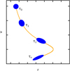 |
Fig. 1 Schematic evolution in phase-space of the distribution of perturbed realisations (purple ellipses) of the dynamics starting from the initial state s0 (yellow curve). |
3 Simulations and results
3.1 Lyapunov spectrum
We integrated a wide range of initial conditions spanning four configurations of the three-body problem. In this work, we present classical and relativistic integrations for a Pythagorean (hereafter pytha), a figure-eight choreography (hereafter fig8) (Moore 1993; Chenciner & Montgomery 2000), and two hierarchical triples, where the outer orbit is either markedly elliptical or quasi-circular with e ≈ 10−4, (hereafter hie1 and hie2, respectively). In Fig. 2, the three particle trajectories are shown with different colours in the classical case.
For all runs, we first evaluated the largest Lyapunov exponent Λmax using its discrete time definition (1). In the classical cases, Λmax was evaluated using both the tangent dynamics given in Eq. (2) and the commonly adopted perturbed trajectory subtraction. We find that, using double precision and a second-order integration scheme, the values of the largest Lyapunov exponent obtained with the two choices are in good agreement when the size of the perturbation in the second method is ≈5 × 10⁻⁶ and the perturbed orbit is re-normalised every 10Δt according to the Benettin et al. (1976) algorithm.
In Figure 3, we show the time series of Λmax(t) for the classical (black lines) and relativistic (purple lines) calculations for the four configurations introduced above. Each value of Λmax (t) is the median value of ten realisations. For all systems, c/v* ≈ 102, while the integration has been stopped when the instantaneous value of Λmax is smaller than 0.5% of its median for at least 5t*. In all test cases shown herein, the 2PN relativistic computation yields a maximal Lyapunov exponent that is smaller than its classical counterpart (i.e. in the limit of c/v* → ∞), corresponding to a longer Lyapunov time, which appears to confirm what was observed by Portegies Zwart et al. (2022) for 1PN perturbations; for example, see their Figures (9) and (10) for the low N cases. A similar picture (not shown here) is also obtained when perturbing the phase-space coordinates of only one of the three initial particles.
However, other choices of c/v* in the relativistic simulations at fixed system orbital parameters yield values of Λmax that may or may not be smaller than what is computed for the classical case. In order to obtain a clearer view of the trends of the Lyapunov exponents with the scaled speed of light, we calculated the first four approximated Lyapunov indicators  (corresponding to the only positive exponents λ1,2,3,4 for the classical three-body problem) using the expression given by Eq. (12) in the range 10 < c/v* < 106. The tensor Ii,j is evaluated in all cases using 103 independent perturbed trajectories iterated for up to 15 units of normalised time, which is much less than the roughly 150t* needed, on average, to converge the series used to evaluate Λmax. Propagating up to larger times would typically hinder the procedure as the instantaneous distribution of orbits in phase-space would most likely no longer be enclosed in a hyperellipsoid, in particular in the markedly chaotic systems. In Fig. 4, we show
  for (from left to right) the pytha, fig8, hie1, and hie2 sets of numerical simulations with 10 < c/v* < 106. For comparison, the horizontal dashed lines mark the value obtained for the purely classical model. As a general trend, all orbital types yield values of
  both larger and smaller than its classical value, with a somewhat common tendency to have larger
  for c/v* → 10 and smaller values for c/v*→ 106. The fig8 and hie1 cases (second and third panel) have values of
  that are systematically lower (except for a few outliers) than for the classical limit, which is indicated by the horizontal dashed line, while for the pytha and hie2 cases, the relativistic
  fall below the classical limit in recognisable intervals of c/v* at around 102 and 103.
Interestingly, a non-monotonic trend of Λmax with the strength of a perturbing term in an N -particle Hamiltonian has also been observed by Di Cintio et al. (2018a, 2019); Dhar et al. (2019) for one-dimensional non-linear lattices. In such cases, the largest Lyapunov exponent plotted as a function of єH for different Ns or specific energy Etot/N presented a well-defined local minimum at a specific value of the perturbation strength. The latter was parametrised there by the exponent α of a power-law extra coupling between lattice nodes (e.g. see Fig. 2 in Di Cintio et al. 2018a or Fig. 8 in Di Cintio et al. 2019). We note that, a different normalisation of the equations of motion would simply shift the position of the relative minima of λ1 , as equal values of c/v* and  would correspond to different total energies in natural units.
The other  are shown in Figure 5 (filled symbols) as functions of the rescaled c against the values obtained in the classical case, which are again marked by the horizontal dashed lines. We observe that, for large values of c/v* (i.e. vanishing PN corrections), all Lyapunov exponents converge to the values obtained in the simulations where the PN terms were switched off. On the other hand, in the limit of small c/v* (corresponding to strong relativistic corrections), the values attained by
  are typically larger than or comparable to their estimated classical values. In the intermediate regime, one or more exponents can be considerably smaller than their counterparts for the parent classical system. Remarkably, the pytha and hie2 sets of simulations (top left and bottom right panels in Fig. 5) yield a distribution of
  showing a strongly non-monotonic trend with c/v*, in particular for
  . In practice, for a given orbital configuration, accounting for the first two PN corrections does not necessarily imply an increase in chaoticity – as one would expect – associated to shorter exponentiation times of the distance of initially nearby trajectories; or at least not in every phase-space direction. When the relativistic corrections are in the regime corresponding to the scaled speed of light, 20 ≲ c/v* ≲ 2 × 10³, the value of the first Lyapunov exponent might be smaller than the classical one, while the second, third, and fourth could instead be slightly larger. Remarkably, the second exponent
  for the Pythagorean problem shows a sharp drop at around c/v* ≈ 103 followed by an increase at c/v* ≈ 300. Therefore, in some cases (cf. again the hie2 runs in Fig. 5 for c/v* ≈ 200), surprisingly, while
  is larger in the PN simulations,
  might be considerably smaller. This diversity in behaviour is summarised in Figure 6, where we show the ratio of the relativistic to classical positive Lyapunov spectra (top panel) as well as the individual values of
  (bottom panel) for the same systems as in Fig. 5 and choices of c/v* indicated by the colour map ranging from light green (corresponding to c/v* ≈ 3.5) to dark blue (corresponding to c/v* ≈ 3 × 10⁶). Again, it appears clear how, for many values of c/v*, even the smaller exponents
  might lower when the PN terms are activated. This implies that there exist systems where chaoticity can indeed be mitigated along multiple phase-space directions other than that associated with Λmax , as reported by Portegies Zwart et al. (2022) for the 1PN corrections.
From the point of view of the orbital structure in configuration space, this can be interpreted as either a stabilising or a destabilising effect induced by the precession caused by the non- dissipative relativistic terms4. As an example, in Fig. 7, for the purely classical and 2PN Pythagorean problem with c/v* ≈ 950, we show the evolution of the distance from the centre of mass of the three particles m1, m2, and m3. In this case (cf. left panel in Fig. 2), the PN terms alter the outcome of the strong encounter happening at t ≈ 58, and so the triplet remains bound for at least another 60 time units. In general, chaos in low-N gravitational systems is ascribed to the superposition of resonances (Mardling 2008, see also Chirikov 1979). For example, hierarchical triplets undergoing the von Zeipel-Lidov-Kozai (ZLK) mechanism (von Zeipel 1910; Lidov 1962; Kozai 1962) are ‘stabilised’ (i.e. the ZLK mechanism is suppressed) by the inclusion of PN terms, because apsidal precession averages the torques on the inner binary to zero (Naoz et al. 2013).
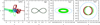 |
Fig. 2 X − Y projections of the classical test orbits in the centre of mass frame for (from left to right) a Pythagorean, a figure-eight, and two hierarchical configurations of the three-body problem. |
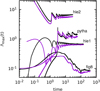 |
Fig. 3 Evolution of the numerical finite maximum Lyapunov exponent over time for four orbits of the classical (black lines) and relativistic 2PN (purple lines) three-body problem with c/v* ≈ 102 . |
 |
Fig. 4 Maximal Lyapunov exponents λ1 as function of the c/v* ratio for (from left to right) a wildly chaotic Pythagorean, a figure-eight, and two hierarchical triplets (symbols). The horizontal dashed lines mark the values for the parent classical systems. |
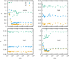 |
Fig. 5 Numerical Lyapunov exponents λ2, λ3, and λ4 as functions of the c/v* ratio for (clockwise top left) a wildly chaotic Pythagorean, a figureeight, and two hierarchical triplets (symbols). The horizontal dashed lines mark the values for the parent classical systems. |
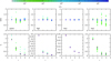 |
Fig. 6 Ratio |

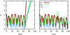 |
Fig. 7 Time-dependent distance R from the centre of mass of the systems for the three masses in a Pythagorean problem without (left panel) and with (right panel) 2PN corrections for c/v* ≈ 950. |
3.2 Dynamical entropy
It appears clear that one cannot rely solely on the first (i.e. maximal) Lyapunov exponent to characterise the ‘amount of chaos’ of a given model under the type of perturbations explored here. In order to refine our quantification of chaos, we evaluated the upper boundary of the KS dynamical entropy as the sum of the  according to Eq. (13). In Figure 8,
  is shown as a function of c/v* for the systems presented in Figs. 4 and 5 and is compared with its classical value, indicated in each of the four panels by a horizontal dashed line. The behaviour of the estimated dynamical entropy confirms that the examined three-body problems exhibit a partial suppression of their chaoticity when the 2PN corrections are turned on, that is, for several values of the normalised c when the latter is between 10 and 3 × 10²; this is particularly evident for the Pythagorean problem (top left panel), where in two definite intervals of c/v*,
  is of a factor of ≈1.2 smaller in the relativistic simulations. The hie2 case also shows a significant drop in
  for c/v* between 10 and 103. For c/v* → 1 (not shown in the plot), we observe a systematic increase in
  that is associated with augmented chaoticity. However, we stress that in the c/v* ≈ 1 limit, the perturbative approach, which is valid for the integration scheme employed here, is no longer consistent. Consequently, the PN terms cannot be considered as ϵH-type perturbations and even the PN expansion itself fails to be a valid approximation of general relativity. Moreover, whether or not other definitions of dynamical entropy – not necessarily associated with the Lyapunov exponents (Kandrup & Mahon 1994) – could yield similar results when applied to PN dynamics remains to be determined.
4 Discussion and conclusions
Prompted by the numerical work of Portegies Zwart et al. (2022) on the relativistic N -problem, we explored the behaviour of the positive part of the Lyapunov spectrum of some configurations of the gravitational three-body problem under the effect of the first and second post-Newtonian (PN) perturbative terms. Our analysis employed three different metrics of chaos, namely the maximal Lyapunov exponent (Figures 3 and 4), the Lyapunov spectra (Figure 5), and the Kolmogorov-Sinai entropy (Figure 8). We applied these chaos indicators to four different configurations of the three-body problem: the Pythagorean configuration (Burkert et al. 2012), the figure-eight Chenciner & Montgomery (2000), and two different configurations of hierarchical triple systems.
The main results of this paper can be summarised as follows:
- 1
Including up to second-order PN terms lowers the largest Lyapunov exponent Λmax in a broad range of values of the parameter c/v* at fixed orbit configuration.
- 2
The values of the other three classical non-negative Lyapunov exponents can be either lower or higher in the relativistic case, regardless of whether Λmax is smaller or larger than its classical counterpart.
- 3
For a given orbital configuration, the dynamical KS entropy exhibits a markedly non-monotonic trend with c/v*, in particular between 10 and ≈103.
These results confirm and strengthen the findings of Portegies Zwart et al. (2022) and Boekholt et al. (2021), as it appears that, not only might the terms proportional to 1/c2 mitigate chaos, but also this intriguing behaviour survives, at least when the second-order 1/c4 PN corrections are turned on. We conjecture that this apparent mitigation of chaos might be ascribed to the relativistic precession that, under certain conditions, softens the otherwise hard particle encounters. As a consequence, N -body models where the PN corrections become important might have a longer (or shorter) chaotic instability timescale associated with the inverse of the largest Lyapunov exponent (Gurzadyan & Savvidy 1986) if the latter are accounted for in the numerical calculations. In particular, in systems dominated by a large central mass, such as the nuclear star clusters (Seth et al. 2008; Antonini 2013; Graham 2016), and where three-body encounters are likely to shape the dynamical evolution, a correct determination of the relativistic chaos suppression or enhancement is therefore needed (Dall’Amico et al. 2024). Moreover, we expect similar implications in the stellar dynamics around binary supermassive black holes, where the diffusion of orbits – studied for example in Kandrup et al. (2003) – should in principle be affected by the PN corrections.
Nevertheless, it remains to be determined whether the behaviour of the three-(and possibly N)body problem with relativistic extra terms could be interpreted in the same way as the models reported by Di Cintio et al. (2018a, 2019), where the transport properties are both quantitatively and qualitatively changed by the specific strength and form of the perturbation (see also Iubini et al. 2018). In particular, the cases corresponding to relative minima of Λmax present energy diffusion patterns akin to those of integrable or nearly integrable systems (cf. Fig. 1 in Di Cintio et al. 2018a). In this regard, it is worth noting that the concept of ‘stabilising perturbations’ was already introduced in the context of the so-called Hamiltonian control by Ciraolo et al. (2004a,b, 2005); Vittot et al. (2005) building on an earlier hypothesis put forward by Gallavotti (1982). As proposed by this latter author, additional perturbative terms are added to a chaotic Hamiltonian in a way that some chaotic orbits are turned into regular or nearly regular orbits, while preserving the large scale structure of phase-space. Interestingly, the requirements of the Hamiltonian control theory are compatible with our picture of the gravitational three-body problem subjected to small relativistic corrections, in the sense that a non-integrable Hamiltonian exhibits a more regular behaviour (i.e. less chaotic) once perturbed with an extra ϵH term. Finally, it would be worth investigating how including higher-order PN terms affects the energy dependence of chaotic three-body encounters within dense stellar systems featuring a central cusp. Specifically, we aim to explore how enhanced or reduced relativistic chaos influences resonant relaxation (Rauch & Tremaine 1996; Sridhar & Touma 2016; Bar-Or & Fouvry 2018; Máthé et al. 2023). A numerical study addressing this question is currently underway. In such endeavours, it is essential to normalise the system such that the proper c/v∗ is derived from individual orbital energies rather than being treated as a free parameter, as done in this work.
 |
Fig. 8 Dynamical entropy |

Acknowledgements
We thank Stefano Ruffo, Simon Portegies-Zwart and Antonio Politi for the stimulating discussion at the initial stage of this project and the anonymous Referee for his/her comments that helped improving the presentation of our results. We acknowledge funding by the “Fondazione Cassa di Risparmio di Firenze” under the project HIPERCRHEL for the use of high performance computing resources at the University of Firenze. AAT acknowledges support from the Horizon Europe research and innovation programs under the Marie Skłodowska-Curie grant agreement no. 101103134. PFDC wishes to thank the hospitality of the Kavli Institute of Theoretical Physics at the University of Santa Barbara where part of the present work was completed.
References
- Ali, Y., & Roychowdhury, S. 2024, arXiv e-prints [arXiv:2408.09011] [Google Scholar]
- Antonini, F. 2013, ApJ, 763, 62 [Google Scholar]
- Bar-Or, B., & Fouvry, J.-B. 2018, ApJ, 860, L23 [NASA ADS] [CrossRef] [Google Scholar]
- Benettin, G., Galgani, L., & Strelcyn, J.-M. 1976, Phys. Rev. A, 14, 2338 [Google Scholar]
- Benettin, G., Galgani, L., Giorgilli, A., & Strelcyn, J. M. 1980, Meccanica, 15, 9 [NASA ADS] [CrossRef] [Google Scholar]
- Binney, J., & Tremaine, S. 2008, Galactic Dynamics, 2nd edn [Google Scholar]
- Blanchet, L. 1996, Phys. Rev. D, 54, 1417 [NASA ADS] [CrossRef] [Google Scholar]
- Blanchet, L. 2024, Liv. Rev. Relativ., 27, 4 [NASA ADS] [CrossRef] [Google Scholar]
- Boccaletti, D., & Pucacco, G. 1999, Theory of Orbits [CrossRef] [Google Scholar]
- Boekholt, T. C. N., Moerman, A., & Portegies Zwart, S. F. 2021, Phys. Rev. D, 104, 083020 [CrossRef] [Google Scholar]
- Boekholt, T. C. N., & Portegies Zwart, S. F. 2023, arXiv e-prints [arXiv:2311.07651] [Google Scholar]
- Boekholt, T. C. N., Portegies Zwart, S. F., & Heggie, D. C. 2023, Int. J. Mod. Phys. D, 32, 2342003 [NASA ADS] [CrossRef] [Google Scholar]
- Burkert, A., Schartmann, M., Alig, C., et al. 2012, ApJ, 750, 58 [CrossRef] [Google Scholar]
- Burrau, C. 1913, Astron. Nachr., 195, 113 [NASA ADS] [CrossRef] [Google Scholar]
- Chenciner, A., & Montgomery, R. 2000, Ann. of Math., 3, 881 [CrossRef] [Google Scholar]
- Chirikov, B. V. 1979, Phys. Rep., 52, 263 [NASA ADS] [CrossRef] [Google Scholar]
- Chitan, A. S., Mylläri, A., & Haque, S. 2022, MNRAS, 509, 1919 [Google Scholar]
- Christiansen, F., & Rugh, H. H. 1997, Nonlinearity, 10, 1063 [NASA ADS] [CrossRef] [Google Scholar]
- Cipriani, P., & Pettini, M. 2003, Ap&SS, 283, 347 [NASA ADS] [CrossRef] [Google Scholar]
- Ciraolo, G., Briolle, F., Chandre, C., et al. 2004a, Phys. Rev. E, 69, 056213 [NASA ADS] [CrossRef] [Google Scholar]
- Ciraolo, G., Chandre, C., Lima, R., Vittot, M., & Pettini, M. 2004b, Celest. Mech. Dyn. Astron., 90, 3 [NASA ADS] [CrossRef] [Google Scholar]
- Ciraolo, G., Chandre, C., Lima, R., et al. 2005, Europhys. Lett., 69, 879 [NASA ADS] [CrossRef] [Google Scholar]
- Contopoulos, G. 2002, Order and chaos in dynamical astronomy [CrossRef] [Google Scholar]
- Dall’Amico, M., Mapelli, M., Torniamenti, S., & Arca Sedda, M. 2024, A&A, 683, A186 [NASA ADS] [CrossRef] [EDP Sciences] [Google Scholar]
- Damour, T., & Deruelle, N. 1985, Ann. Inst. Henri Poincare Sect. A Phys. Theor., 43, 107 [NASA ADS] [Google Scholar]
- Dhar, A., Kundu, A., Lebowitz, J. L., & Scaramazza, J. A. 2019, J. Statist. Phys., 175, 1298 [NASA ADS] [CrossRef] [Google Scholar]
- Di Cintio, P., & Casetti, L. 2019, MNRAS, 489, 5876 [NASA ADS] [CrossRef] [Google Scholar]
- Di Cintio, P., & Casetti, L. 2020a, MNRAS, 494, 1027 [NASA ADS] [CrossRef] [Google Scholar]
- Di Cintio, P., & Casetti, L. 2020b, in Star Clusters: From the Milky Way to the Early Universe, 351, eds. A. Bragaglia, M. Davies, A. Sills, & E. Vesperini, 426 [NASA ADS] [Google Scholar]
- Di Cintio, P., Iubini, S., Lepri, S., & Livi, R. 2018a, Chaos Solitons Fractals, 117, 249 [NASA ADS] [CrossRef] [Google Scholar]
- Di Cintio, P., Rossi, A., & Valsecchi, G. B. 2018b, in International Astronauti- cal Federation (IAF), 19, Proceedings of the 68th International Astronautical Congress (IAC 2017). 25–29 September 2017, Adelaide, Australia Curran Associates Inc., 267 [Google Scholar]
- Di Cintio, P., Iubini, S., Lepri, S., & Livi, R. 2019, J. Phys. A Math. Gen., 52, 274001 [NASA ADS] [CrossRef] [Google Scholar]
- Dubeibe, F. L., Lora-Clavijo, F. D., & González, G. A. 2017a, Ap&SS, 362, 97 [NASA ADS] [CrossRef] [Google Scholar]
- Dubeibe, F. L., Lora-Clavijo, F. D., & González, G. A. 2017b, Phys. Lett. A, 381, 563 [NASA ADS] [CrossRef] [Google Scholar]
- Einstein, A., Infeld, L., & Hoffmann, B. 1938, Ann. Math., 39, 65 [NASA ADS] [CrossRef] [Google Scholar]
- El-Zant, A. A. 2002, MNRAS, 331, 23 [CrossRef] [Google Scholar]
- El-Zant, A. A., Everitt, M. J., & Kassem, S. M. 2019, MNRAS, 484, 1456 [NASA ADS] [CrossRef] [Google Scholar]
- Fodor, G., Hoenselaers, C., & Perjés, Z. 1989, J. Math. Phys., 30, 2252 [CrossRef] [Google Scholar]
- Gallavotti, G. 1982, Commun. Math. Phys., 87, 365 [NASA ADS] [CrossRef] [Google Scholar]
- Goodman, J., Heggie, D. C., & Hut, P. 1993, ApJ, 415, 715 [Google Scholar]
- Graham, A. W. 2016, in Galactic Bulges, part of the book series Astrophysics and space science library (Berlin: Springer Nature), 312, 269 [Google Scholar]
- Gurzadyan, V. G., & Savvidy, G. K. 1986, A&A, 160, 203 [NASA ADS] [Google Scholar]
- Gurzadyan, V. G., & Kocharyan, A. A. 2009, A&A, 505, 625 [NASA ADS] [CrossRef] [EDP Sciences] [Google Scholar]
- Habib, S., Kandrup, H. E., & Elaine Mahon, M. 1997, ApJ, 480, 155 [NASA ADS] [CrossRef] [Google Scholar]
- Heggie, D. C., & Mathieu, R. D. 1986, in The Use of Supercomputers in Stellar Dynamics, 267, eds. P. Hut, & S. L. W. McMillan, 233 [NASA ADS] [CrossRef] [Google Scholar]
- Hemsendorf, M., & Merritt, D. 2002, ApJ, 580, 606 [NASA ADS] [CrossRef] [Google Scholar]
- Hut, P., Makino, J., & McMillan, S. 1995, ApJ, 443, L93 [NASA ADS] [CrossRef] [Google Scholar]
- Iubini, S., Di Cintio, P., Lepri, S., Livi, R., & Casetti, L. 2018, Phys. Rev. E, 97, 032102 [NASA ADS] [CrossRef] [Google Scholar]
- Kandrup, H. E., & Mahon, M. E. 1994, A&A, 290, 762 [NASA ADS] [Google Scholar]
- Kandrup, H. E., & Sideris, I. V. 2001, Phys. Rev. E, 64, 056209 [NASA ADS] [CrossRef] [Google Scholar]
- Kandrup, H. E., & Siopis, C. 2003, MNRAS, 345, 727 [Google Scholar]
- Kandrup, H. E., & Smith, Haywood, J. 1991, ApJ, 374, 255 [NASA ADS] [CrossRef] [Google Scholar]
- Kandrup, H. E., Sideris, I. V., & Bohn, C. L. 2001, Phys. Rev. E, 65, 016214 [NASA ADS] [CrossRef] [Google Scholar]
- Kandrup, H. E., Sideris, I. V., Terzic, B., & Bohn, C. L. 2003, ApJ, 597, 111 [NASA ADS] [CrossRef] [Google Scholar]
- Kinoshita, H., Yoshida, H., & Nakai, H. 1991, Celest. Mech. Dyn. Astron., 50, 59 [NASA ADS] [CrossRef] [Google Scholar]
- Kol, B. 2023, Celest. Mech. Dyn. Astron., 135, 29 [NASA ADS] [CrossRef] [Google Scholar]
- Kolmogorov, A. 1958, Dokl. Akad. Nauk SSSR, 119, 861 [Google Scholar]
- Kolmogorov, A. 1959, Dokl. Akad. Nauk SSSR, 124, 754 [Google Scholar]
- Komatsu, N., Kiwata, T., & Kimura, S. 2009, Physica A Statist. Mech. Appl., 388, 639 [CrossRef] [Google Scholar]
- Kovács, T., Bene, G., & Tél, T. 2011, MNRAS, 414, 2275 [CrossRef] [Google Scholar]
- Kozai, Y. 1962, AJ, 67, 591 [Google Scholar]
- Lichtenberg, A., & Lieberman, M. 1992, Regular and Chaotic Dynamics [CrossRef] [Google Scholar]
- Lidov, M. L. 1962, Planet. Space Sci., 9, 719 [Google Scholar]
- Maindl, T. I., & Dvorak, R. 1994, A&A, 290, 335 [NASA ADS] [Google Scholar]
- Mardling, R. A. 2008, in IAU Symposium, 246, Dynamical Evolution of Dense Stellar Systems, eds. E. Vesperini, M. Giersz, & A. Sills, 199 [NASA ADS] [Google Scholar]
- Máthé, G., Szölgyén, Á., & Kocsis, B. 2023, MNRAS, 520, 2204 [CrossRef] [Google Scholar]
- Mei, L., & Huang, L. 2018, Comput. Phys. Commun., 224, 108 [NASA ADS] [CrossRef] [Google Scholar]
- Mikkola, S., & Merritt, D. 2006, MNRAS, 372, 219 [NASA ADS] [CrossRef] [Google Scholar]
- Miller, R. H. 1964, ApJ, 140, 250 [NASA ADS] [CrossRef] [Google Scholar]
- Miller, R. H. 1971, J. Computat. Phys., 8, 449 [NASA ADS] [CrossRef] [Google Scholar]
- Moore, C. 1993, Phys. Rev. Lett., 70, 3675 [NASA ADS] [CrossRef] [Google Scholar]
- Mora, T., & Will, C. M. 2004, Phys. Rev. D, 69, 104021 [CrossRef] [Google Scholar]
- Naoz, S., Kocsis, B., Loeb, A., & Yunes, N. 2013, ApJ, 773, 187 [NASA ADS] [CrossRef] [Google Scholar]
- Ovod, D. V., & Ossipkov, L. P. 2013, Astron. Nachr., 334, 800 [NASA ADS] [CrossRef] [Google Scholar]
- Pesin, Y. B. 1977, Russ. Math. Surveys, 32, 55 [NASA ADS] [CrossRef] [Google Scholar]
- Portegies Zwart, S., & Boekholt, T. 2014, ApJ, 785, L3 [NASA ADS] [CrossRef] [Google Scholar]
- Portegies Zwart, S. F., Boekholt, T. C. N., Por, E. H., Hamers, A. S., & McMillan, S. L. W. 2022, A&A, 659, A86 [NASA ADS] [CrossRef] [EDP Sciences] [Google Scholar]
- Quarles, B., Eberle, J., Musielak, Z. E., & Cuntz, M. 2011, A&A, 533, A2 [NASA ADS] [CrossRef] [EDP Sciences] [Google Scholar]
- Rauch, K. P., & Tremaine, S. 1996, New A, 1, 149 [NASA ADS] [CrossRef] [Google Scholar]
- Rein, H., & Tamayo, D. 2016, MNRAS, 459, 2275 [Google Scholar]
- Roy, A. E. 2005, Orbital motion [Google Scholar]
- Seth, A., Agüeros, M., Lee, D., & Basu-Zych, A. 2008, ApJ, 678, 116 [NASA ADS] [CrossRef] [Google Scholar]
- Sideris, I. V., & Kandrup, H. E. 2002, Phys. Rev. E, 65, 066203 [NASA ADS] [CrossRef] [Google Scholar]
- Sinai, Y. 1959, Dokl. Akad. Nauk SSSR, 124, 768 [Google Scholar]
- Sitnikov, K. 1960, Dokl. Akad. Nauk SSSR, 133, 303 [Google Scholar]
- Skokos, C. 2001, J. Phys. A Math. Gen., 34, 10029 [Google Scholar]
- Skokos, C. 2010, in Lecture Notes in Physics, Berlin Springer Verlag, 790, eds. J. Souchay, & R. Dvorak, 63 [NASA ADS] [CrossRef] [Google Scholar]
- Soffel, M. H. 1989, Relativity in Astrometry, Celestial Mechanics and Geodesy [Google Scholar]
- Spurzem, R., Berentzen, I., Berczik, P., et al. 2008, Parallelization, Special Hardware and Post-Newtonian Dynamics in Direct N-Body Simulations, eds. S. J. Aarseth, C. A. Tout, & R. A. Mardling (Dordrecht: Springer Netherlands), 377 [Google Scholar]
- Sridhar, S., & Touma, J. R. 2016, MNRAS, 458, 4143 [CrossRef] [Google Scholar]
- Steklain, A. F., & Letelier, P. S. 2006, Phys. Lett. A, 352, 398 [NASA ADS] [CrossRef] [Google Scholar]
- Terzić, B., & Kandrup, H. E. 2003, Phys. Lett. A, 311, 165 [CrossRef] [Google Scholar]
- Trani, A. A., Leigh, N. W. C., Boekholt, T. C. N., & Portegies Zwart, S. 2024, A&A, 689, A24 [NASA ADS] [CrossRef] [EDP Sciences] [Google Scholar]
- Valtonen, M. J., Mikkola, S., & Pietila, H. 1995, MNRAS, 273, 751 [NASA ADS] [CrossRef] [Google Scholar]
- Vittot, M., Chandre, C., Ciraolo, G., & Lima, R. 2005, Nonlinearity, 18, 423 [NASA ADS] [CrossRef] [Google Scholar]
- von Zeipel, H. 1910, Astron. Nachr., 183, 345 [Google Scholar]
- Wiesel, W. E. 1993, Phys. Rev. E, 47, 3686 [Google Scholar]
- Wolf, A., Swift, J. B., Swinney, H. L., & Vastano, J. A. 1985, Physica D Nonlinear Phenomena, 16, 285 [NASA ADS] [CrossRef] [Google Scholar]
- Yoshida, H. 1990, Phys. Lett. A, 150, 262 [NASA ADS] [CrossRef] [Google Scholar]
- Yoshida, H. 1993, Celest. Mech. Dyn. Astron., 56, 27 [NASA ADS] [CrossRef] [Google Scholar]
We note that the softening of the gravitational forces at vanishing interparticle distance might affect the dependence of the Lyapunov exponents on the model’s resolution, as shown by Komatsu et al. (2009).
Remarkably, Ali & Roychowdhury (2024) recently observed that the Poincaré sections of stellar orbits in the relative potential of rotating galactic supermassive black holes have a smaller chaotic region than the parent classical setup when the relativistic terms are accounted for. Vice versa, the Smaller Alignment Index (SALI, Skokos 2001, a quantity related to the Lyapunov exponents) is systematically larger for the relativistic cases.
We note that, in the relativistic case, the conserved quantities have a different form (Mora & Will 2004).
The 1 and 2PN terms affect the precession frequency in a binary interaction, while the following 2.5PN term associated with the gravitational wave emission induces the decay of the semi-major axis (Mora & Will 2004).
All Figures
|
Fig. 1 Schematic evolution in phase-space of the distribution of perturbed realisations (purple ellipses) of the dynamics starting from the initial state s0 (yellow curve). |
| In the text | |
|
Fig. 2 X − Y projections of the classical test orbits in the centre of mass frame for (from left to right) a Pythagorean, a figure-eight, and two hierarchical configurations of the three-body problem. |
| In the text | |
|
Fig. 3 Evolution of the numerical finite maximum Lyapunov exponent over time for four orbits of the classical (black lines) and relativistic 2PN (purple lines) three-body problem with c/v* ≈ 102 . |
| In the text | |
|
Fig. 4 Maximal Lyapunov exponents λ1 as function of the c/v* ratio for (from left to right) a wildly chaotic Pythagorean, a figure-eight, and two hierarchical triplets (symbols). The horizontal dashed lines mark the values for the parent classical systems. |
| In the text | |
|
Fig. 5 Numerical Lyapunov exponents λ2, λ3, and λ4 as functions of the c/v* ratio for (clockwise top left) a wildly chaotic Pythagorean, a figureeight, and two hierarchical triplets (symbols). The horizontal dashed lines mark the values for the parent classical systems. |
| In the text | |
|
Fig. 6 Ratio |
| In the text | |
|
Fig. 7 Time-dependent distance R from the centre of mass of the systems for the three masses in a Pythagorean problem without (left panel) and with (right panel) 2PN corrections for c/v* ≈ 950. |
| In the text | |
|
Fig. 8 Dynamical entropy |
| In the text | |
Current usage metrics show cumulative count of Article Views (full-text article views including HTML views, PDF and ePub downloads, according to the available data) and Abstracts Views on Vision4Press platform.
Data correspond to usage on the plateform after 2015. The current usage metrics is available 48-96 hours after online publication and is updated daily on week days.
Initial download of the metrics may take a while.