| Issue |
A&A
Volume 698, June 2025
|
|
|---|---|---|
| Article Number | A258 | |
| Number of page(s) | 11 | |
| Section | Stellar structure and evolution | |
| DOI | https://doi.org/10.1051/0004-6361/202554183 | |
| Published online | 17 June 2025 | |
Discerning internal conditions of pulsating hot subdwarf B-type stars
Modeling multiple trapped modes in KIC 10001893
1
Independent Scholar, 9000 Ghent, Belgium
2
Institute of Astronomy, KU Leuven, Celestijnenlaan 200D, 3001 Leuven, Belgium
3
Astrophysics group, Department of Physics, University of Surrey, Guildford GU2 7XH, United Kingdom
4
Max-Planck-Institut für Astrophysik, Karl-Schwarzschild-Straße 1, 85741 Garching bei München, Germany
5
Radboud University Nijmegen, Department of Astrophysics, IMAPP, P.O. Box 9010 6500 GL Nijmegen, The Netherlands
6
Max Planck Institute for Astronomy, Koenigstuhl 17, 69117 Heidelberg, Germany
⋆ Corresponding author: This email address is being protected from spambots. You need JavaScript enabled to view it.
Received:
19
February
2025
Accepted:
13
May
2025
Abstract
Context. The frequencies of gravity-mode oscillations are determined by the chemical, thermal, and structural properties of stellar interiors, which facilitates the study of internal mixing mechanisms in stars. We investigated the impact of discontinuities in the chemical composition induced by the formation of an adiabatic semi-convection region during the core helium (He)-burning phase of evolution of hot subdwarf B-type (sdB) stars.
Aims. This study delves into the progression of convective core evolution, using a numerical approach to model the emergence of a semi-convection zone. We scrutinize the asteroseismic attributes of the evolutionary stages and assess the core He-burning phase by evaluating the parameter linked to the average interval between the deep trapped modes in both sdB evolutionary models and the observations of KIC 10001893.
Methods. We performed evolutionary and asteroseismic analyses of sdB stars using MESA and GYRE to examine the properties of the semi-convection region. Additionally, we computed parameters related to gravity-mode period spacings and the interval between deep trapped modes to characterize the core He-burning phase at different stages of sdB evolution.
Results. Using a numerical scheme in MESA to model the development of the semi-convection zone, we illustrate the evolution of the convective core in sdB stars. Our study addresses the challenges of relying solely on the average interval between oscillation mode periods with consecutive radial orders to identify the core He-burning stage. To improve identification, we propose a new parameter that represents the average interval between deep trapped modes during some of the stages of sdB evolutionary models. Additionally, we find that integrating convective penetration with convective premixing improves our models and yields comparable outcomes without the need for additional model parameters.
Conclusions. Our results can advance the development of detailed evolutionary models for sdB stars by refining internal mixing schemes, increasing the accuracy of pulsation predictions, and improving alignment with observational data.
Key words: asteroseismology / stars: evolution / stars: horizontal-branch / stars: interiors / stars: oscillations / subdwarfs
© The Authors 2025
 Open Access article, published by EDP Sciences, under the terms of the Creative Commons Attribution License (https://creativecommons.org/licenses/by/4.0), which permits unrestricted use, distribution, and reproduction in any medium, provided the original work is properly cited.
This article is published in open access under the Subscribe to Open model. This email address is being protected from spambots. You need JavaScript enabled to view it. to support open access publication.
1. Introduction
Hot subdwarf B-type (sdB) stars are believed to be core helium (He)-burning stars and are characterized by an exceedingly thin hydrogen (H) envelope, with an envelope mass less than 0.02 times the mass of the Sun. Their average mass aligns closely with the mass threshold at which the core-He flash occurs, approximately 0.47 times the mass of the Sun (Fontaine et al. 2012). These sdB stars represent evolved, compact entities with surface gravities (log g) ranging from 5.2 to 6.2 dex, effective temperatures (Teff) from 20 000 to 40 000 K, and radii from 0.10 R⊙ to 0.30 R⊙ (Heber 2016). They occupy the intermediate phase between the main sequence and the cooling stage of white dwarfs, known as the extreme horizontal branch (EHB; see Heber 2016 for a detailed review).
The evolutionary trajectory of sdB stars requires substantial mass loss, primarily driven by binary interactions during the late stages of the red giant phase (Paczynski 1976; Han et al. 2002, 2003; Pelisoli et al. 2021). This phase leads to the removal of nearly all of the H-rich envelope, resulting in a core that burns He but possesses an envelope too thin to sustain H-shell burning. Over a period of roughly 108 years, sdB stars continue to burn He in their cores. Upon the exhaustion of the He in their core, they progress into a phase during which He is burned in a shell surrounding a core composed of carbon and oxygen (C/O), evolving into subdwarf O-type (sdO) stars. Ultimately, these stars end their life cycle as white dwarfs (Dorman et al. 1993). This exotic evolutionary pathway affords us the opportunity to directly observe and scrutinize the properties of the mixed He-C/O cores of low- and intermediate-mass stars, which are otherwise obscured by a thick hydrogen envelope.
Kilkenny et al. (1997) were the first to discover rapid pulsations in a subgroup of hot sdB stars, now termed V361 Hya stars but commonly known as short-period sdB variable (sdBV) stars. These stars exhibit multiple pulsation periods ranging from 60 s to 800 s, which correspond to low-degree (ℓ ≲ 3), low-order (0 ≤ n ≲ 20) pressure modes (p modes) within this frequency range. The excitation of these modes is attributed to a classical κ-mechanism, primarily driven by the accumulation of iron group elements, particularly iron itself, in a region known as the Z bump. This mechanism was proposed by Charpinet et al. (1996, 1997), who showed that radiative levitation enhances the concentrations of iron group elements, a prerequisite for activating the pulsational modes. The p-mode sdB pulsators typically populate a temperature range of 28 000 K to 35 000 K, with surface gravities between log g of 5 and 6 dex. Following this discovery, another class of sdB pulsators displaying long-period pulsations, termed V1093 Her stars, was identified by Green et al. (2003). These stars exhibit brightness variations with periods extending to a few hours. The oscillation frequencies observed in these pulsators are associated with low-degree (ℓ < 3) and medium- to high-order (10 < n < 60) gravity modes (g modes) and are driven by the same κ-mechanism due to the accumulation of iron group elements, as outlined by Fontaine et al. (2003), Jeffery & Saio (2006a,b, 2007), and Charpinet et al. (2011). In contrast to p-mode sdB pulsators, g-mode sdB pulsators exhibit somewhat cooler temperatures, ranging from 22 000 K to 30 000 K, with surface gravities (log g) typically falling within 5.0 dex to 5.5 dex. Within the group of pulsating sdB stars, there is a subset known as “hybrid” sdB pulsators that exhibit both g and p modes concurrently (e.g., Schuh et al. 2006). These hybrid sdB pulsators have Teff of 28 000 K to 32 000 K. These objects are particularly significant as they offer a unique opportunity for asteroseismic investigations, enabling the study of both the core structure and the outer layers of sdBV stars.
The advancements in high-precision and high-duty-cycle photometric monitoring from space missions such as the Kepler mission (Borucki et al. 2010) and the TESS (Transiting Exoplanet Survey Satellite) mission (Ricker et al. 2014) have led to the identification of new candidates of pulsating sdB stars. As a result, over 300 pulsating sdB stars have been found and documented thus far (Uzundag et al. 2024). These missions have not only been effective in identifying new candidates of pulsating sdB stars but have also enabled unprecedented asteroseismic measurements. For instance, seismic tools such as rotational multiplets and asymptotic period spacings can now be used (see Reed et al. 2018 and Lynas-Gray 2021 for a review).
Throughout the horizontal branch (HB) phase, the interaction between layers rich in C/O and those rich in He causes a change in the chemical composition at the core boundary. In models, the size of the core during the HB phase can either increase or remain unchanged depending on how the transport or mixing of chemical species near the convective core is modeled i.e., in 1D or multidimensional approaches, which have been debated at length in the literature (Salaris & Cassisi 2017; Paxton et al. 2019; Herwig et al. 2023; Blouin et al. 2024). Various mixing mechanisms have been proposed, such as semi-convection, convective penetration, and convective overshooting (Castellani et al. 1985; Mowlavi & Forestini 1994; Bossini et al. 2015; Schindler et al. 2015; Constantino et al. 2015; Schindler et al. 2017; Xiong et al. 2017; Li et al. 2018; Guo 2018; Johnston et al. 2024). In addition to the chemical mixing outside of the core, the method for determining the location of the convective boundary introduces uncertainty into evolutionary calculations. Some numerical approaches to modeling mixing processes in stellar evolution attempt to represent the emergence of adiabatic semi-convection regions that extend beyond traditional convection (Paxton et al. 2019; Castellani et al. 1985; Mowlavi & Forestini 1994). Semi-convection persists during the He-burning phase, with the semi-convective region achieving convective neutrality throughout the core, including at its edge. Maintaining the balance of He, C, and O within this semi-convective zone is crucial as it regulates the necessary adjustment in the radiative gradient of this region. The development of adiabatic semi-convection beyond the convective core presents a promising alternative to overshooting approaches. This method effectively circumvents issues such as convective shell formation. The precise effects of various mixing scenarios and their corresponding numerical methods remain a topic of debate. However, current research is revealing promising new approaches, two of which involve modeling the R2 ratio, which compares the number of stars observed during the early asymptotic giant branch phase to those in the HB phase (Constantino et al. 2016, 2017; Ghasemi et al. 2017) and asteroseismology.
The non-radial oscillations observed in pulsating sdB stars offer a unique way to probe their internal properties if their pulsation geometry can be determined (Aerts et al. 2010). Space observations have facilitated the identification of oscillation modes via pattern recognition, a capability that has not been widely achievable with ground-based data. This development has had a profound impact on theoretical models, particularly in areas where the physics related to chemical mixing (especially diffusion, overshooting, and semi-convection) is poorly constrained. Exploring pulsating compact stars, particularly sdB stars, offers a unique approach to understanding mixing mechanisms in the vicinity of their core and envelope through asteroseismology (Charpinet et al. 2002a,b, 2011; Van Grootel et al. 2008, 2010a,b; Hu et al. 2007, 2008, 2009, 2010, 2011; Bloemen et al. 2014). In particular, the power of modeling pulsations has already been shown to enable the characterization of the chemical profile and mixing mechanisms in sdB stars (Constantino et al. 2015; Ghasemi et al. 2017; Charpinet et al. 2019; Ostrowski et al. 2021). Asymptotic period sequences, particularly for dipole (ℓ = 1) and quadrupole (ℓ = 2) modes of consecutive radial order, have proven effective for analyzing the g-mode pulsations in observed sdBV stars; over 60% of the periodicities have been attributed to these modes (e.g., Reed et al. 2011; Uzundag et al. 2021). However, the sdB stars are characterized by layers of varying composition, some of which result from mixing mechanisms near their cores. This complexity complicates the straightforward application of the asymptotic approximations typically used for homogeneous stars. These compositional discontinuities cause deviations from sequences expected for homogeneous stars. Such disruptions have been observed in several pulsating sdB stars. Furthermore, as these compositional discontinuities intensify in the transition zones within the stars due to the mixing process, certain modes can become deeply trapped near the convective core (Constantino et al. 2015; Ghasemi et al. 2017; Ostrowski et al. 2021; Guyot et al. 2025). This phenomenon has also been identified in a few pulsating sdB stars observed by Kepler (Østensen et al. 2014; Uzundag et al. 2017).
Throughout the nominal Kepler mission, a total of 18 pulsating sdB stars were observed in short-cadence mode. The majority (16) exhibit long-period g-mode pulsations, with only two showing short-period p-mode pulsations. Furthermore, three previously identified sdB stars within the open cluster NGC 6791 were discovered to pulsate (Reed et al. 2018). In this study, we focused on modeling a pulsating sdB star, namely KIC 10001893, one of the field sdB stars that underwent extensive monitoring by the Kepler spacecraft. The spectroscopic atmospheric parameters of KIC 10001893, as provided by Østensen et al. (2011), including Teff = 26 700 ± 300 K, log g = 5.30 ± 0.04, and log(NHe/NH) = − 2.09 ± 0.1, are strongly indicative of alignment with the g-mode instability strip (Silvotti et al. 2014). Frequency analysis of KIC 10001893 unveiled 110 oscillation peaks. A comprehensive seismic analysis of KIC 10001893 was conducted by Uzundag et al. (2017), revealing 32 ℓ = 1 and 18 ℓ = 2 modes. The authors also discovered the presence of nearly complete sequences of consecutive radial orders for both ℓ = 1 and ℓ = 2 modes, which included three deep trapped modes. These trapped modes were clearly visible in the reduced-period diagram, which displayed an almost perfect alignment of the two sequences. The locations of these deep trapped modes, along with the spacing between them, provide invaluable information for examining the stellar interior and evaluating various mixing models in the vicinity of the core boundary.
This paper is organized as follows. Section 2 presents the three models for convective core evolution in sdB stars. The first, the sign-change algorithm, utilizes overshooting and detects convective boundaries using either the Schwarzschild criterion or the Ledoux criterion. The predictive mixing (PM) numerical model extends convective regions until the boundaries meet convectivity conditions on the convective side of the core within a single time step. The convective premixing (CPM) scheme employs a numerical approach to model the emergence of the adiabatic semi-convection zone during the core He-burning phase. Section 2 also describes the evolution and formation of sdB stars, as well as the evolution of the convective core incorporating the CPM scheme. Section 3 describes the asteroseismic properties of sdB models that employ the CPM scheme. In Sect. 4 we investigate the asteroseismic properties of sdB models with time-dependent convective penetration in conjunction with the CPM scheme. Finally, in Sect. 5 we discuss our findings and potential future directions. The CPM scheme and the convective penetration implementation in MESA models for sdB stars are publicly available on GitHub1.
2. Models of convective cores in evolutionary models of sdB stars
We calculated stellar structure and evolution models using the 1D Modules for Experiments in Stellar Astrophysics (MESA) code (Paxton et al. 2011, 2013, 2015, 2018, 2019; Jermyn et al. 2023). Determining the location of convective boundaries during both the core H- and He-burning phases is a complex subject. Paxton et al. (2019) discusses three numerical methods available in MESA: the sign-change algorithm and the PM and CPM schemes (see Fig. 1). The details of our computational models of sdB stars using MESA are discussed in Appendix A. The simple sign-change method for determining convective boundaries involves detecting sign changes in the variable y using either the Schwarzschild criterion (y = ∇rad − ∇ad) or the Ledoux criterion (y = ∇rad − ∇L). Here, ∇rad, ∇ad, and ∇L represent the radiative, adiabatic, and Ledoux temperature gradients, respectively. However, this approach may fail in circumstances with composition discontinuities, particularly when the radiative gradient ∇rad exceeds the adiabatic gradient ∇ad on the convective side of the core (Gabriel et al. 2014). In the outer region of the convective core, overshooting leads to increased transfer of C and O into the radiative part, consequently increasing opacities. Additionally, following Kramer’s law, temperature decreases toward the outer part of the convective core, further increasing opacity and ∇rad in these outer regions. In the subsequent evolutionary stages, convective regions located below the outer convective layers exhibit lower ∇rad, transitioning to a radiative state, while convective shells form simultaneously in the outer regions (see Fig. 1a). In the top panel of Fig. 2, the green plot illustrates the convective shell where ∇rad is greater than ∇ad.
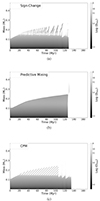 |
Fig. 1. Schematic representation of the interior structures of an sdB star, displaying the logarithm of the diffusion coefficient for mixing during the core He-burning stage. Different levels of mixing are indicated by the grayscale bar on the right-hand y-axis. The panels show the results of the sign-change numerical method (a), the PM scheme (b), and the CPM scheme (c). Gray denotes convective core regions, with the hatched area in panel (c) indicating semi-convection in the transitional zone between convective and radiative regions. |
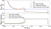 |
Fig. 2. Top panel: Adiabatic gradient (blue) and radiative gradients for three distinct sdB models – sign-change (green), PM (red), and CPM (black) – plotted as a function of the mass coordinate at 80 Myr. Bottom panel: He mass fraction corresponding to the temperature gradients of each of the three models. |
Another numerical approach, the PM scheme, improves the sign-change algorithm by extending convective regions until the boundaries satisfy ∇rad = ∇ad on the convective side within a single time step (see Fig. 1b). This numerical method is modified to prevent the initial splitting of a convection region. During the PM iterations, if at any point within the convective region ∇rad = ∇ad, the code restricts further growth of that convection region. The PM has demonstrated its effectiveness in achieving the desired objective of preventing the formation of convective shells above the convective core. Nevertheless, as illustrated in the top panel of Fig. 2 (red), in this numerical method, the persistence of ∇rad > ∇ad on the convective side of the convective boundary highlights the necessity for further exploration of mixing models (Gabriel et al. 2014).
As illustrated in Fig. 1c, the CPM scheme provides an alternative numerical technique for modeling mixing beyond convection in stellar evolution, avoiding issues found in previously discussed numerical methods (Paxton et al. 2019). It is performed at the beginning of each time step before any structural or chemical modifications occur. The CPM extends convective boundaries until the radiative gradient equals the adiabatic gradient on the convective side of the boundary. This stage is often accompanied by the initial appearance of convective shells, which in the CPM scheme gradually merge into the semi-convective zone. The convective shells with shorter mixing timescales approach convective neutrality first. This process continues until all convective shells reach neutrality, causing the breakdown of earlier convective layers and the expansion of the semi-convective zone. A mesh cell above the convective boundary may become convective, while a cell within the convective zone may revert to a radiative state. This process repeats until the outer boundary cells of the convective zone stabilize in radiative states after mixing. Mixing within the mesh cells assumes constant pressure and temperature in each cell, requiring updates to abundances, densities, opacities, and temperature gradients (including radiative, adiabatic, and Ledoux gradients) within the affected cells. Overall, this numerical scheme creates classical semi-convection regions, where the abundance gradient is adjusted to maintain convective neutrality (∇rad = ∇ad) located above the convective core, as depicted in the upper panel of Fig. 2. The balance of He, C, and O in the semi-convective area is critical, as it dictates the necessary decrease in the radiative gradient within the region. The CPM scheme appears to be a promising substitute for the offered two numerical methods, which suffer from problems such as the appearance of the convective shell and having ∇rad > ∇ad on the convective side of the convective core boundary (see the black line in the upper panel of Fig. 2). As a result, we decided to apply the CPM scheme in all models used in our research.
A thorough understanding of the precursor phases leading to the evolution and formation of sdB stars is essential for studying these stellar objects. This study employs the MESA algorithm to model the evolution of single stars, as shown in Fig. 1 of Ghasemi et al. (2017). The star evolves from the pre-main-sequence phase to the tip of the red giant branch. The core of the star contracts during the red giant branch evolutionary process, which reduces the mean separation between the constituent particles. Subsequently, as the core contracts and releases gravitational energy, an electron-degenerate He core is formed.
To replicate the effects of binary interaction and envelope mass stripping that lead to the formation of an sdB star, the relax_mass option in MESA is utilized. This approach involves the incorporation of a high mass-loss rate starting at the tip of the red giant branch. After the process of envelope mass stripping, the resulting model resembles an sdB star, typically with a mass of around 0.47 M⊙ and a very low envelope mass, such as 0.002 M⊙. In the subsequent phase, the onset of successive core He flashes occurs. The weak interaction of neutrinos with matter facilitates the effective cooling of the central regions within the degenerate He core. As the He flashes occur, nearly 5 percent of the He fuses into C and O. The energy liberated by these nuclear processes elevates the core temperature, consequently augmenting the de Broglie wavelength of the electrons. This action removes the electron degeneracy from the He core. The inward progression of the He flashes continues over approximately 2 million years (Bildsten et al. 2012; Ghasemi et al. 2017). Ultimately the core contracts, stable He-burning through the triple-alpha reaction yields C during the EHB phase.
During the EHB phase, the convective core progresses in distinct stages, each with its own unique characteristics, instead of progressing uniformly. Overall, we can identify three distinct stages in its evolution. Calculations performed using another code, STELUM, also reveal nearly the same three main stages during the He-burning phase (Giammichele et al. 2022). The initial stage spans from the zero-age EHB to the point where nearly 30% of the core He is consumed. During this phase, the convective core expands consistently (that can be seen in stellar ages from 0 to roughly 20 million years in Fig. 1c), and there is no requirement for a semi-convective region. The neutrality condition (∇rad = ∇ad) persists on the convective side of the core boundary, as depicted in the top panel of Fig. 3.
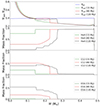 |
Fig. 3. Top panel: Adiabatic gradient (blue) and radiative gradients for three distinct sdB models depicted in Fig. 1c, all plotted as mass coordinates. These models are differentiated by their respective ages: 15 million years (My) shown in green, 75 My in red, and 120 My in black. Bottom panels, from top to bottom: He, C, and O mass fractions corresponding to each of the sdB models in the top panel. |
The second stage lasts until approximately 10% of the He remains in the core (as seen in stellar ages from nearly 20 to roughly 110 million years in the bottom panel of Fig. 1). To meet the neutrality condition (∇rad = ∇ad), the quantities of He, C, and O must be adjusted appropriately at each point within the semi-convection region. This involves adjusting the chemical composition to maintain a temperature gradient that closely matches the adiabatic gradient, as illustrated in red in the top panels of Fig. 3. This numerical approach succeeds in the primary phase of central He-burning when the amount of O produced is not yet substantial.
The third stage is known as breathing pulses. These pulses arise from the efficient nuclear transformation of C into O. Since O has a higher opacity than C, this transformation leads to an increase in opacity, which in turn creates a higher radiative gradient, depicted in black in the top panel of Fig. 3. As a result, the convective core expands largely, enabling the mixing of large quantities of He into the burning zone. After this expansion, the core contracts over a short evolutionary timescale, leading to several evolutionary phases marked by smaller, growing convective cores that resemble the initial stage, free from the semi-convective region, as shown in Fig. 1c at the end of core He-burning phase. The breathing pulses are recurring events significantly influenced by mixing processes near the convective core and by the numerical methods used to apply these processes at the convective boundary. If the boundary of the convective core reaches the outer layers of He at sufficiently low temperatures, pulses can occur before the nuclear fuel in the core is depleted. Otherwise, the He-burning phase ends.
3. Deciphering the asteroseismic properties of sdB models
According to asymptotic analysis, high-order g modes should have periods that are equally spaced in chemically homogeneous nonrotating nonmagnetic stars (Tassoul 1980). However, the measured period spacings of g modes are known to be nonuniform. These deviations can be employed to more thoroughly understand the properties of the stellar interior, particularly the interior chemical mixing characteristics (Miglio et al. 2008).
In order to comprehend the structure of compact evolved stars, the period spacing between p and g modes has been studied. The asymptotic theory analysis of white dwarfs with an outer convection zone and a discontinuity in their chemical composition was developed by Brassard et al. (1992a,b). The asymptotic theory for the case of sdB stars with a convective core and a radiative envelope was introduced by Charpinet et al. (2000, 2002a,b).
In Fig. 4a, the Kiel diagram displays the relationship between stellar gravities (log g) and effective temperatures (Teff) for the CPM scheme. The spectroscopic properties of KIC 10001893 are depicted in green, accompanied by error bars. Eight models labeled A to H with varying ages (10, 27, 41, 62, 78, 97, 125, and 134 million years) represent all three evolutionary stages discussed earlier. Model A represents the initial uniform growing convective core phase, while models B to F mark the second evolutionary phase with a semi-convection region. Model G corresponds to the breathing pulses phase, and point H denotes the end of the He-burning phase. These models are also featured in Fig. 4b, which illustrates the schematic representation of sdB star interior structures during the He-burning stage using the CPM scheme.
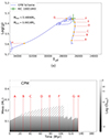 |
Fig. 4. Panel (a): Kiel diagram of stellar gravity (log g) against effective temperature (Teff) for the CPM scheme. The position of KIC 10001893 is illustrated in green with error bars. Eight models with different ages (A = 10 My, B = 27, C = 41, D = 62, E = 78, F = 97, G = 125, and H = 134 million years) are indicated. Panel (b): Same as Fig. 1c, hatched areas indicate semi-convection in the transitional zone between the convective (gray) and radiative (white) regions. All eight models from the top panel are also shown in this panel. |
Different mixing methods yield unique configurations of the chemical gradient around the convective core, impacting the period spacing pattern. Therefore, the observed period spacing patterns provide the potential to improve our understanding of the mixing dynamics near the convective core and the effectiveness of the mixing mechanisms.
The boundary layer between the C/O core and the He shell has a significant impact on the period spacing patterns. Moreover, the semi-convection zone depicted in light gray in Fig. 4b can generate deep mode trapping patterns. A sharp composition gradient marks the boundary between the semi-convection zone and the outer radiative layer. The semi-convection region occupies the space between this boundary and the lower boundary of the convective core.
Figure 5 illustrates the period spacing of KIC 10001893 in blue, contrasted with the red period spacings of the eight models featured in Fig. 4. The semi-convection generates intricate deep-mode trapping patterns. As the evolutionary path progresses, the distance between the sharp composition gradients in the outer semi-convection area and the lower convective core increases, leading to an increase in the number of trapped modes. Consequently, at model A, where the semi-convection area is absent, deep trapped modes do not exist, and the period spacing solely relies on the He/H transition layer and the sharp composition gradient at the top of the convective core boundary. As the size of the semi-convection region increases from models B through F, the number of deeply trapped modes also rises. Furthermore, the spacing between these trapped modes remains relatively constant over this range. However, this pattern changes at models G and H, where the distances between the deeply trapped modes are no longer uniform.
The top of Fig. 6a illustrates the periodic spacing pattern of g modes with a degree of ℓ = 1 and consecutive radial order n for a stellar model employing the CPM scheme, corresponding to the model F in Figs. 4 and 5. The radial orders of six modes are denoted by black-filled arrows. Changes in the chemical gradients alter the density profile and, consequently, the Brunt-Väisälä frequency. Within the sdB models, transitions from H to He in the outer envelope and from He to C/O near the convective boundary create distinct features in the Brunt–Väisälä frequency, as indicated by the blue solid line in Fig. 6b. The analysis reveals that the horizontal component of the eigen-displacements, ξh, depicted by the red line in Fig. 6b for modes with radial orders n = 15, 29, 37, are confined in the vicinity of the Brunt–Väisälä frequency peak near the core. Certain displacement eigenfunctions, with nodes situated very close to the semi-convective zones, exhibit significant amplitudes inside the semi-convection regions, shown by the red solid line in Fig. 6b for modes with radial orders n = 19, 25, 32.
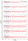 |
Fig. 5. Measured period spacing of KIC 10001893 (blue) and the period spacings of the eight models depicted in Fig. 4 (red). The order of the panels corresponds to the model ages, with the youngest at the top and the oldest at the bottom. |
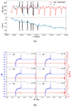 |
Fig. 6. Top of panel (a): Period spacing pattern of g modes with degree ℓ = 1 and consecutive radial order n for a stellar model employing the CPM scheme, corresponding to point F in Fig. 4. Radial orders for six modes are indicated by black arrows. Bottom of panel (a): Normalized mode inertia plotted against the periods of the dipole (ℓ = 1) g modes. Panel (b): Horizontal displacement eigenfunctions (ξh) of the dipole g modes plotted as a function of the mass coordinate for various radial orders, as referenced in the top panels. Red lines represent the eigenfunctions, and blue lines the Brunt-Väisälä frequency within the stellar interior. |
The normalized inertia of these modes represents the average kinetic energy associated with displacement eigenfunctions across time. The bottom of Fig. 6a shows the normalized mode inertia plotted against the period of the dipole (ℓ = 1) g modes. In the CPM scheme, a few modes with large amplitudes become trapped within the semi-convective area. Consequently, these deep trapped modes display significant mode inertias, as indicated by the filled black arrows in Fig. 6a (bottom), for modes with radial orders n = 19, 25, 32.
One of the lower panels in Fig. 5 illustrates the period spacing of model G, which is associated with the breathing pulses. Seismic measurements of the central oxygen abundance in white dwarfs point to the occurrence of breathing pulses in the cores of their progenitors during the He-burning phase (Giammichele et al. 2022). This highlights the importance of breathing pulses in stellar models. In this phase, as C undergoes efficient conversion into O within the core, the opacity increases, leading to a rise in the radiative gradient. This, in turn, triggers a sudden expansion of the convective core, followed by the emergence of a Brunt–Väisälä frequency peak in the outer radiative region. Subsequently, there is a contraction, resulting in the appearance of Brunt–Väisälä frequency peaks in the inner radiative region, eventually leading to the formation of a small growing convective core. The presence of multiple Brunt–Väisälä frequency peaks above the expanding convective core can give rise to irregular patterns in trapped modes, where modes with nodes close to these peaks become trapped. Due to the varied distances between these peaks, the average interval between the trapped modes and the trapping depth of these modes can differ, causing irregularities in the pattern of trapped modes. At model H in Fig. 5, which corresponds to the end of He-burning, the period spacing decreases as the convective core size shrinks.
The red dots in the top panel of Fig. 7 illustrate a new parameter that signifies the average interval between deep trapped modes during the second stage of the sdB evolution, as elaborated in Sect. 2. The observed mean distances between three deep trapped modes of KIC 10001893 are denoted by a blue line. Moving to the middle panel of Fig. 7, the red dots display the mean period spacings excluding deep trapped modes in both the first and second evolutionary stages of the sdB evolution, as elaborated in Sect. 2. Meanwhile, the observed mean period spacing of KIC 10001893, excluding three deep trapped modes and three semi-trapped modes, is represented by a blue line. Lastly, the bottom panel of Fig. 7 showcases the mean period spacing throughout all evolutionary stages of He-burning of the sdB, as illustrated by red dots. The observed mean period spacing of KIC 10001893 is displayed by a blue line.
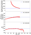 |
Fig. 7. Top panel: Average interval between the deep trapped modes during the second stage of evolving the sdB models for the CPM scheme, as shown in Fig. 4b by red dots, and the observed mean distances between three deep trapped modes of KIC 10001893, depicted with a blue line. Middle panel: Mean period spacing without considering the deep trapped modes in the first and second evolutionary stages of the sdB models, illustrated by red dots. The blue line represents the observed mean period spacing, excluding three deep trapped modes and three semi-trapped modes of KIC 10001893. Bottom panel: Mean period spacing of all modes in all the evolutionary stages of He-burning of the sdB models, as depicted by red dots. The blue line displays the observed mean period spacing of all modes of KIC 10001893. |
As shown in the lower panel of Fig. 7, it becomes apparent that using the mean period spacing of all modes as a parameter to define the core He-burning phase during the second stage of sdB evolution is impractical. Throughout the majority of this phase, the mean period spacing of all modes remains relatively constant. Even when considering the mean period spacing for modes not trapped in the semi-convection region, without accounting for the deep trapped modes and semi-trapped modes in this region, discerning a clear pattern for the last part of the second stage of He-burning becomes challenging. This is primarily due to the inconsistency in the stability of the convective core boundary, resulting in fluctuations in the mean period spacing, as depicted in the middle panel of Fig. 7. Furthermore, as shown in the lower panel of Fig. 7, it is clear that using the mean period spacing during the first stage of sdB evolution remains reliable.
In our sdB models, we identify deep trapped modes within the semi-convective region by their horizontal displacement, which are required to exceed 0.5R* within that region. As shown in Fig. 6b, the modes with radial orders 19, 25, and 32 all have horizontal displacements above this threshold within the semi-convective zones. As depicted in the top panel of Fig. 7, utilizing the average interval parameter between deep trapped modes proves to be an effective means of distinguishing the core He-burning phase. Throughout the second stage of He-burning, the average interval parameter exhibits a consistent decrease as the age increases, displaying a steady decline without fluctuations. Consequently, the average interval parameter emerges as a reliable metric for characterizing the He-burning phase within our sdB evolutionary models. Notably, we refrain from specifying the average interval parameter for the third evolutionary stage, the breathing pulses, due to the almost negligible presence of the semi-convection region and the irregular pattern of the trapped modes during this phase.
4. Time-dependent convective penetration
Johnston et al. (2024) described how the dissipation-balanced convective penetration procedure, initially developed in 3D numerical simulations by Anders et al. (2022), was implemented into the MESA 1D stellar evolution model. Jermyn et al. (2022) employed a similar approach to estimate the penetration zone (PZ) in the post-processing step while ignoring the effects of the PZ on the evolution of stars.
Multidimensional hydrodynamic simulations consistently reveal the emergence of a convective PZ, where the temperature gradient shifts smoothly from ∇rad to ∇ad. In this section we utilize this methodology alongside the CPM scheme to demonstrate evolutionary and asteroseismic outcomes when incorporating mixing beyond the convective core without introducing additional free parameters to our models. This algorithm is founded on the concept that convective parcels extend beyond boundaries due to velocity and inertia, leading to convective penetration. The algorithm calculates the extent of this PZ above the convective boundary by balancing buoyant work against dissipative forces, assuming full mixing with an adiabatic temperature gradient. This time-dependent convective penetration algorithm calculates the extent of the PZ at each time step of the evolution using the properties of the star, unlike previous methods, which remove free parameters and determine the PZ according to the properties of the model as a post-processing step (Jermyn et al. 2022).
The insights from 3D hydro simulations are derived, as described by Anders et al. (2022), to characterize the dissipation profile within the PZ and the dissipation-to-buoyant work ratio in the convective zone. These findings are then included in the 1D MESA code. Furthermore, the temperature gradient within the convective zone and PZ is adjusted to replicate the adiabatic gradient and smoothly transition to the radiative gradient via the Péclet number (Michielsen et al. 2021). The Péclet number is a dimensionless measure that compares the thermal diffusion timescale to the convective turnover time to describe the relative importance of convective and radiative heat transport (Jermyn et al. 2022).
Figure 8a provides a schematic representation of the internal structures of the sdB star during the He-burning phase, highlighting the phenomenon of convective penetration.
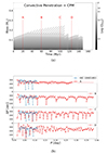 |
Fig. 8. Panel (a): Schematic representation of the sdB star’s interior structures for the logarithm of the diffusion coefficient of mixing during the core He-burning stage, using convective penetration combined with the CPM scheme. Different levels of mixing are indicated by the grayscale bar on the right-hand y-axis. The hatched area represents semi-convection in the transitional zone between the convective (gray) and radiative (white) regions. The figure shows four points with varied ages (A = 20, B = 60, C = 100, and D = 127 million years). Panel (b): Period spacing of KIC 10001893 (blue) and the period spacings of the four models depicted in panel (a) (red). The order of the panels corresponds to their ages, with the youngest at the top and the oldest at the bottom. |
Figure 8a illustrates the convective penetration situated between the convective core and the radiative and semi-convective regions. Alternatively, the convective penetration can be substituted with overshooting, or the overshooting can be introduced above the convective penetration (see Michielsen et al. 2021), yielding similar outcomes. In Fig. 8b the period spacings of the models exhibit a consistent pattern reminiscent of those observed in the CPM scheme, albeit without the presence of convective penetration as shown in Figs. 4 and 5. Most modes, except for the deep trapped ones, reflect off the outer boundary of the semi-convective region. Only the deep trapped modes penetrate this region; therefore, the mean period spacing for non-trapped modes depends on the size of this boundary, which is the same for both model C in Fig. 8a and model F in Fig. 4b. On the other hand, the size of the semi-convective region reflects the depth of the deep trapped modes. As our models age, the semi-convective region grows. Since the depth of the deep trapped modes is nearly identical in the two models, model C in Fig. 8a, which has a larger convective core due to its convective penetration region, occurs later, around 100 million years, compared to model F in Fig. 4b, which occurs at approximately 97 million years.
At the end of the He-burning phase, due to the different number and sizes of breathing pulses, the fully enriched C/O core and the abundance gradient region below the fully He-rich layers differ in size and compositional structure between the models in Fig. 4b and those in Fig. 8a.
5. Discussion and conclusion
Our research focused on the evolution of the convective core in sdB stars, revealing a nonuniform progression marked by three distinct stages in the CPM scheme (Paxton et al. 2019; Ostrowski et al. 2021). The CPM scheme uses a numerical approach to model the formation of the adiabatic semi-convection zone during the core He-burning phase (Castellani et al. 1985; Mowlavi & Forestini 1994). Static asteroseismic models predict convective core masses significantly higher than those suggested by the CPM scheme (Van Grootel et al. 2010b,a; Charpinet et al. 2011, 2019). In these models, the He–H transition layer and the deep core boundary layers play a key role in mode trapping, as discussed extensively by Guyot et al. (2025), to which we refer for details. In the models examined in this study, variations in chemical composition caused by the CPM scheme within the transition zones near the cores of sdB stars lead to certain modes becoming strongly trapped and displaying similar depths and intervals. This phenomenon is supported by Kepler space-telescope observations of particular sdB stars (Østensen et al. 2014; Uzundag et al. 2021).
Gabriel et al. (2014) suggested that in the context of the sign-change numerical approach, the persistent dominance of ∇rad > ∇ad on the convective side of the core boundary underscores the need for additional mixing mechanisms to be considered, such as adiabatic semi-convection. The sign-change can anticipate the emergence of multiple peaks in the Brunt–Väisälä frequency above the expanding convective core during specific phases of the second evolutionary stage. Such occurrences could lead to irregularities in the intervals and depths of the deep trapped modes (Ghasemi et al. 2017). In the second evolutionary stage, the premixing technique predicts a single Brunt–Väisälä peak at the outer boundary of the semi-convection region, which traps modes. Consequently, the CPM scheme yields nearly identical estimates for the average interval between deep trapped modes and the depth of all these modes. According to Uzundag et al. (2017), observations support the presence of three deep trapped modes, as confirmed by the mode period spacing with ℓ = 1; two of these deep trapped modes were re-confirmed with ℓ = 2 and exhibit identical depths, which is consistent with the CPM scheme predictions.
Blouin et al. (2024) conducted a 3D simulation study of the He-burning phase in a 3 M⊙ red clump star, exploring CPM and PM numerical approaches at the convective core boundary. However, they find that the semi-convection region between the convective core and the radiative envelope exhibits insufficient mixing due to internal gravity waves, contrary to the claim by Herwig et al. (2023). Nonetheless, their simulation suggests that convective intrusion and overshooting could potentially eliminate this region within just 10–50 convective turnover timescales. Extrapolating entrainment over evolutionary timescales might further erase this semi-convection region. In scenarios involving the PZ and the application of the CPM, employing higher mesh densities can introduce fluctuations during the second stage of He-burning, a phase during which our study anticipates smooth growth in semi-convective regions. After these fluctuations, the semi-convective region re-forms, suggesting that the simulation in Blouin et al. (2024) might be based on one of these minor variations. Additionally, according to Blouin et al. (2024), an incomplete representation could lead to an overestimation of the rate at which semi-convection is eroded. Most importantly, according to this study, the PM numerical approach results are not consistent with the g-mode asteroseismology of sdB stars and cannot explain the regions that cause deep trapped g modes. Multidimensional hydrodynamics simulations consistently indicate the formation of a convective PZ, where the temperature gradient smoothly transitions from ∇rad to ∇ad. This behavior aligns with the modeling we outline in Sect. 4.
Variations in the initial masses of sdB stars during their main sequence and red giant phases, combined with mass loss due to binary system interactions, can result in a wide range of total and envelope masses (Hu et al. 2007, 2008). This, in turn, influences the structure of the transition layer between He and H near the envelope, leading to variations in the Brunt-Väisälä peak. As the initial mass escalates from 1 M⊙ to 2.5 M⊙, the transition layer between He and H becomes smoother and broader, resulting in a lower and broader peak in the Brunt-Väisälä frequency. Consequently, there are fewer and less noticeable ordinary trapped modes in the period spacing pattern. However, the pattern of deep trapped modes remains the same.
Our future research will focus on constructing comprehensive grids of evolutionary models for sdB stars, which is crucial for determining the parameters of observed pulsating sdB stars. By testing various envelope masses and structures of the He-H transition layer, and assuming the CPM scheme is at play above the convective core, we can improve the accuracy of pulsation predictions. The growing number of observed pulsating sdB stars, particularly with continuous high-precision space photometry, holds promise for identifying an increased proportion of sdB stars exhibiting trapped modes. This advancement can empower us to harness the pulsations of sdB stars, refining the determination of parameters for observed pulsating sdB stars, particularly when encountering trapped mode patterns. In addition, observing more sdB stars in clusters can increase our accuracy when determining their parameters using the CPM scheme. Since pulsating sdB stars within a single cluster all have the same distance and composition, they offer additional constraints for parameter determination through asteroseismic grid modeling. The ages inferred from the zero-age main sequence are approximately the same for all sdB stars within a cluster. However, it is important to note that the ages differ when determined from the onset of core He-burning as the stars within a cluster do not evolve into sdB stars at one particular time. Rather, this onset is determined by the birth mass of the star. Moreover, the ratio of sdB stars to sdO stars in clusters aids in estimating the lifetime of sdB stars during the core He-burning phase relative to the lifetime of sdO stars in the shell He-burning phase. This estimation heavily relies on the overall duration of the breathing pulses and the accuracy of the CPM scheme.
Acknowledgments
M. U. gratefully acknowledges funding from the Research Foundation Flanders (FWO) by means of a junior postdoctoral fellowship (grant agreement No. 1247624N). C.J. acknowledges funding from the Royal Society through the Newton International Fellowship funding scheme (project No.NIF∖R1∖242552). CA received funding from the European Research Council (ERC) under the Horizon Europe programme (Synergy Grant agreement N°101071505: 4D-STAR). While partially funded by the European Union, views and opinions expressed are however those of the author(s) only and do not necessarily reflect those of the European Union or the European Research Council. Neither the European Union nor the granting authority can be held responsible for them.
References
- Aerts, C., Christensen-Dalsgaard, J., & Kurtz, D. W. 2010, Asteroseismology (Springer) [Google Scholar]
- Anders, E. H., Jermyn, A. S., Lecoanet, D., & Brown, B. P. 2022, ApJ, 926, 169 [NASA ADS] [CrossRef] [Google Scholar]
- Angulo, C., Arnould, M., Rayet, M., et al. 1999, Nucl. Phys. A, 656, 3 [Google Scholar]
- Asplund, M., Grevesse, N., Sauval, A. J., & Scott, P. 2009, ARA&A, 47, 481 [NASA ADS] [CrossRef] [Google Scholar]
- Bildsten, L., Paxton, B., Moore, K., & Macias, P. J. 2012, ApJ, 744, L6 [NASA ADS] [CrossRef] [Google Scholar]
- Bloemen, S., Hu, H., Aerts, C., et al. 2014, A&A, 569, A123 [NASA ADS] [CrossRef] [EDP Sciences] [Google Scholar]
- Blouin, S., Shaffer, N. R., Saumon, D., & Starrett, C. E. 2020, ApJ, 899, 46 [NASA ADS] [CrossRef] [Google Scholar]
- Blouin, S., Herwig, F., Mao, H., Denissenkov, P., & Woodward, P. R. 2024, MNRAS, 527, 4847 [Google Scholar]
- Borucki, W. J., Koch, D., Basri, G., et al. 2010, Science, 327, 977 [Google Scholar]
- Bossini, D., Miglio, A., Salaris, M., et al. 2015, MNRAS, 453, 2290 [Google Scholar]
- Brassard, P., Fontaine, G., Wesemael, F., & Hansen, C. J. 1992a, ApJS, 80, 369 [NASA ADS] [CrossRef] [Google Scholar]
- Brassard, P., Fontaine, G., Wesemael, F., & Tassoul, M. 1992b, ApJS, 81, 747 [NASA ADS] [CrossRef] [Google Scholar]
- Burgers, J. M. 1969, Flow Equations for Composite Gases (New York: Academic Press) [Google Scholar]
- Cassisi, S., Potekhin, A. Y., Pietrinferni, A., Catelan, M., & Salaris, M. 2007, ApJ, 661, 1094 [NASA ADS] [CrossRef] [Google Scholar]
- Castellani, V., Chieffi, A., Tornambe, A., & Pulone, L. 1985, ApJ, 296, 204 [Google Scholar]
- Charpinet, S., Fontaine, G., Brassard, P., & Dorman, B. 1996, ApJ, 471, L103 [Google Scholar]
- Charpinet, S., Fontaine, G., Brassard, P., et al. 1997, ApJ, 483, L123 [Google Scholar]
- Charpinet, S., Fontaine, G., Brassard, P., & Dorman, B. 2000, ApJS, 131, 223 [Google Scholar]
- Charpinet, S., Fontaine, G., Brassard, P., & Dorman, B. 2002a, ApJS, 139, 487 [Google Scholar]
- Charpinet, S., Fontaine, G., Brassard, P., & Dorman, B. 2002b, ApJS, 140, 469 [CrossRef] [Google Scholar]
- Charpinet, S., Van Grootel, V., Fontaine, G., et al. 2011, A&A, 530, A3 [NASA ADS] [CrossRef] [EDP Sciences] [Google Scholar]
- Charpinet, S., Brassard, P., Fontaine, G., et al. 2019, A&A, 632, A90 [NASA ADS] [CrossRef] [EDP Sciences] [Google Scholar]
- Chugunov, A. I., Dewitt, H. E., & Yakovlev, D. G. 2007, Phys. Rev. D, 76, 025028 [NASA ADS] [CrossRef] [Google Scholar]
- Constantino, T., Campbell, S. W., Christensen-Dalsgaard, J., Lattanzio, J. C., & Stello, D. 2015, MNRAS, 452, 123 [Google Scholar]
- Constantino, T., Campbell, S. W., Lattanzio, J. C., & van Duijneveldt, A. 2016, MNRAS, 456, 3866 [Google Scholar]
- Constantino, T., Campbell, S. W., & Lattanzio, J. C. 2017, MNRAS, 472, 4900 [NASA ADS] [CrossRef] [Google Scholar]
- Cyburt, R. H., Amthor, A. M., Ferguson, R., et al. 2010, ApJS, 189, 240 [NASA ADS] [CrossRef] [Google Scholar]
- Dorman, B., Rood, R. T., & O’Connell, R. W. 1993, ApJ, 419, 596 [NASA ADS] [CrossRef] [Google Scholar]
- Ferguson, J. W., Alexander, D. R., Allard, F., et al. 2005, ApJ, 623, 585 [Google Scholar]
- Fontaine, G., Brassard, P., Charpinet, S., et al. 2003, ApJ, 597, 518 [Google Scholar]
- Fontaine, G., Brassard, P., Charpinet, S., et al. 2012, A&A, 539, A12 [NASA ADS] [CrossRef] [EDP Sciences] [Google Scholar]
- Freytag, B., Ludwig, H. G., & Steffen, M. 1996, A&A, 313, 497 [NASA ADS] [Google Scholar]
- Fuller, G. M., Fowler, W. A., & Newman, M. J. 1985, ApJ, 293, 1 [NASA ADS] [CrossRef] [Google Scholar]
- Gabriel, M., Noels, A., Montalbán, J., & Miglio, A. 2014, A&A, 569, A63 [NASA ADS] [CrossRef] [EDP Sciences] [Google Scholar]
- Ghasemi, H., Moravveji, E., Aerts, C., Safari, H., & Vučković, M. 2017, MNRAS, 465, 1518 [Google Scholar]
- Giammichele, N., Charpinet, S., & Brassard, P. 2022, Front. Astron. Space Sci., 9, 879045 [NASA ADS] [CrossRef] [Google Scholar]
- Green, E. M., Fontaine, G., Reed, M. D., et al. 2003, ApJ, 583, L31 [Google Scholar]
- Guo, J.-J. 2018, ApJ, 866, 58 [NASA ADS] [CrossRef] [Google Scholar]
- Guyot, N., Van Grootel, V., Charpinet, S., et al. 2025, A&A, 696, A13 [NASA ADS] [CrossRef] [EDP Sciences] [Google Scholar]
- Han, Z., Podsiadlowski, P., Maxted, P. F. L., Marsh, T. R., & Ivanova, N. 2002, MNRAS, 336, 449 [Google Scholar]
- Han, Z., Podsiadlowski, P., Maxted, P. F. L., & Marsh, T. R. 2003, MNRAS, 341, 669 [NASA ADS] [CrossRef] [Google Scholar]
- Heber, U. 2016, PASP, 128, 082001 [Google Scholar]
- Herwig, F. 2000, A&A, 360, 952 [NASA ADS] [Google Scholar]
- Herwig, F., Woodward, P. R., Mao, H., et al. 2023, MNRAS, 525, 1601 [NASA ADS] [CrossRef] [Google Scholar]
- Hu, H., Nelemans, G., Østensen, R., et al. 2007, A&A, 473, 569 [NASA ADS] [CrossRef] [EDP Sciences] [Google Scholar]
- Hu, H., Dupret, M. A., Aerts, C., et al. 2008, A&A, 490, 243 [NASA ADS] [CrossRef] [EDP Sciences] [Google Scholar]
- Hu, H., Nelemans, G., Aerts, C., & Dupret, M. A. 2009, A&A, 508, 869 [NASA ADS] [CrossRef] [EDP Sciences] [Google Scholar]
- Hu, H., Glebbeek, E., Thoul, A. A., et al. 2010, A&A, 511, A87 [NASA ADS] [CrossRef] [EDP Sciences] [Google Scholar]
- Hu, H., Tout, C. A., Glebbeek, E., & Dupret, M. A. 2011, MNRAS, 418, 195 [NASA ADS] [CrossRef] [Google Scholar]
- Iglesias, C. A., & Rogers, F. J. 1993, ApJ, 412, 752 [Google Scholar]
- Iglesias, C. A., & Rogers, F. J. 1996, ApJ, 464, 943 [NASA ADS] [CrossRef] [Google Scholar]
- Irwin, A. W. 2004, The FreeEOS Code for Calculating the Equation of State for Stellar Interiors [Google Scholar]
- Itoh, N., Hayashi, H., Nishikawa, A., & Kohyama, Y. 1996, ApJS, 102, 411 [NASA ADS] [CrossRef] [Google Scholar]
- Jeffery, C. S., & Saio, H. 2006a, MNRAS, 371, 659 [NASA ADS] [CrossRef] [Google Scholar]
- Jeffery, C. S., & Saio, H. 2006b, MNRAS, 372, L48 [NASA ADS] [CrossRef] [Google Scholar]
- Jeffery, C. S., & Saio, H. 2007, MNRAS, 378, 379 [NASA ADS] [CrossRef] [Google Scholar]
- Jermyn, A. S., Schwab, J., Bauer, E., Timmes, F. X., & Potekhin, A. Y. 2021, ApJ, 913, 72 [NASA ADS] [CrossRef] [Google Scholar]
- Jermyn, A. S., Anders, E. H., Lecoanet, D., & Cantiello, M. 2022, ApJ, 929, 182 [NASA ADS] [CrossRef] [Google Scholar]
- Jermyn, A. S., Bauer, E. B., Schwab, J., et al. 2023, ApJS, 265, 15 [NASA ADS] [CrossRef] [Google Scholar]
- Johnston, C., Michielsen, M., Anders, E. H., et al. 2024, ApJ, 964, 170 [NASA ADS] [Google Scholar]
- Kilkenny, D., Koen, C., O’Donoghue, D., & Stobie, R. S. 1997, MNRAS, 285, 640 [Google Scholar]
- Langanke, K., & Martínez-Pinedo, G. 2000, Nucl. Phys. A, 673, 481 [NASA ADS] [CrossRef] [Google Scholar]
- Li, Y., Chen, X.-H., Xiong, H.-R., et al. 2018, ApJ, 863, 12 [NASA ADS] [CrossRef] [Google Scholar]
- Lynas-Gray, A. E. 2021, Front. Astron. Space Sci., 8, 19 [NASA ADS] [Google Scholar]
- Michielsen, M., Aerts, C., & Bowman, D. M. 2021, A&A, 650, A175 [NASA ADS] [CrossRef] [EDP Sciences] [Google Scholar]
- Miglio, A., Montalbán, J., Noels, A., & Eggenberger, P. 2008, MNRAS, 386, 1487 [Google Scholar]
- Mowlavi, N., & Forestini, M. 1994, A&A, 282, 843 [NASA ADS] [Google Scholar]
- Oda, T., Hino, M., Muto, K., Takahara, M., & Sato, K. 1994, At. Data Nucl. Data Tables, 56, 231 [NASA ADS] [CrossRef] [Google Scholar]
- Østensen, R. H., Silvotti, R., Charpinet, S., et al. 2011, MNRAS, 414, 2860 [CrossRef] [Google Scholar]
- Østensen, R. H., Telting, J. H., Reed, M. D., et al. 2014, A&A, 569, A15 [NASA ADS] [CrossRef] [EDP Sciences] [Google Scholar]
- Ostrowski, J., Baran, A. S., Sanjayan, S., & Sahoo, S. K. 2021, MNRAS, 503, 4646 [Google Scholar]
- Paczynski, B. 1976, in Structure and Evolution of Close Binary Systems, eds. P. Eggleton, S. Mitton, & J. Whelan, IAU Symp., 73, 75 [NASA ADS] [CrossRef] [Google Scholar]
- Paxton, B., Bildsten, L., Dotter, A., et al. 2011, ApJS, 192, 3 [Google Scholar]
- Paxton, B., Cantiello, M., Arras, P., et al. 2013, ApJS, 208, 4 [Google Scholar]
- Paxton, B., Marchant, P., Schwab, J., et al. 2015, ApJS, 220, 15 [Google Scholar]
- Paxton, B., Schwab, J., Bauer, E. B., et al. 2018, ApJS, 234, 34 [NASA ADS] [CrossRef] [Google Scholar]
- Paxton, B., Smolec, R., Schwab, J., et al. 2019, ApJS, 243, 10 [Google Scholar]
- Pelisoli, I., Neunteufel, P., Geier, S., et al. 2021, Nat. Astron., 5, 1052 [NASA ADS] [CrossRef] [Google Scholar]
- Potekhin, A. Y., & Chabrier, G. 2010, Contrib. Plasma Phys., 50, 82 [NASA ADS] [CrossRef] [Google Scholar]
- Poutanen, J. 2017, ApJ, 835, 119 [NASA ADS] [CrossRef] [Google Scholar]
- Reed, M. D., Baran, A., Quint, A. C., et al. 2011, MNRAS, 414, 2885 [Google Scholar]
- Reed, M. D., Baran, A. S., Telting, J. H., et al. 2018, Open Astron., 27, 157 [Google Scholar]
- Reimers, D. 1975, Memoires of the Societe Royale des Sciences de Liege, 8, 369 [Google Scholar]
- Ricker, G. R., Winn, J. N., Vanderspek, R., et al. 2014, in Space Telescopes and Instrumentation 2014: Optical, Infrared, and Millimeter Wave, eds. J. M. Oschmann, Jr., M. Clampin, G. G. Fazio, & H. A. MacEwen, Int. Soc. Opt. Photon. (SPIE), 9143, 914320 [NASA ADS] [CrossRef] [Google Scholar]
- Rogers, F. J., & Nayfonov, A. 2002, ApJ, 576, 1064 [Google Scholar]
- Salaris, M., & Cassisi, S. 2017, Royal Soc. Open Sci., 4, 170192 [Google Scholar]
- Saumon, D., Chabrier, G., & van Horn, H. M. 1995, ApJS, 99, 713 [NASA ADS] [CrossRef] [Google Scholar]
- Schindler, J.-T., Green, E. M., & Arnett, W. D. 2015, ApJ, 806, 178 [Google Scholar]
- Schindler, J.-T., Green, E. M., & Arnett, W. D. 2017, Eur. Phys. J. Web Conf., 160, 04001 [Google Scholar]
- Schuh, S., Huber, J., Dreizler, S., et al. 2006, A&A, 445, L31 [NASA ADS] [CrossRef] [EDP Sciences] [Google Scholar]
- Silvotti, R., Charpinet, S., Green, E., et al. 2014, A&A, 570, A130 [NASA ADS] [CrossRef] [EDP Sciences] [Google Scholar]
- Tassoul, M. 1980, ApJS, 43, 469 [Google Scholar]
- Thoul, A. A., Bahcall, J. N., & Loeb, A. 1994, ApJ, 421, 828 [Google Scholar]
- Timmes, F. X., & Swesty, F. D. 2000, ApJS, 126, 501 [NASA ADS] [CrossRef] [Google Scholar]
- Townsend, R. H. D., & Teitler, S. A. 2013, MNRAS, 435, 3406 [Google Scholar]
- Townsend, R. H. D., Goldstein, J., & Zweibel, E. G. 2018, MNRAS, 475, 879 [Google Scholar]
- Uzundag, M., Baran, A. S., Østensen, R. H., et al. 2017, MNRAS, 472, 700 [CrossRef] [Google Scholar]
- Uzundag, M., Vučković, M., Németh, P., et al. 2021, A&A, 651, A121 [NASA ADS] [CrossRef] [EDP Sciences] [Google Scholar]
- Uzundag, M., Krzesinski, J., Pelisoli, I., et al. 2024, A&A, 684, A118 [NASA ADS] [CrossRef] [EDP Sciences] [Google Scholar]
- Van Grootel, V., Charpinet, S., Fontaine, G., et al. 2008, A&A, 488, 685 [NASA ADS] [CrossRef] [EDP Sciences] [Google Scholar]
- Van Grootel, V., Charpinet, S., Fontaine, G., et al. 2010a, ApJ, 718, L97 [NASA ADS] [CrossRef] [Google Scholar]
- Van Grootel, V., Charpinet, S., Fontaine, G., Green, E. M., & Brassard, P. 2010b, A&A, 524, A63 [NASA ADS] [CrossRef] [EDP Sciences] [Google Scholar]
- Xiong, H., Chen, X., Podsiadlowski, P., Li, Y., & Han, Z. 2017, A&A, 599, A54 [NASA ADS] [CrossRef] [EDP Sciences] [Google Scholar]
Appendix A: Computational models of sdB stars
We employed version r23.05.1 of the MESA code (Paxton et al. 2011, 2013, 2015, 2018, 2019; Jermyn et al. 2023) to compute the evolutionary models of sdB stars. We used GYRE version 7.2.1 to calculate the adiabatic eigenfrequencies and eigenfunctions for the normal oscillation modes of the MESA models (Townsend & Teitler 2013; Townsend et al. 2018). The following input physics were used to evolve an sdB model from the pre-main-sequence phase to the end of core He-burning in the EHB phase. The initial stellar mass used in our modeling of sdB stars, during the pre-main-sequence and main-sequence phases, is 1.5 M⊙.
The MESA equation of state (EOS) incorporates a combination of the OPAL (Rogers & Nayfonov 2002), SCVH (Saumon et al. 1995), FreeEOS (Irwin 2004), HELM (Timmes & Swesty 2000), PC (Potekhin & Chabrier 2010), and Skye (Jermyn et al. 2021) EOSs. Radiative opacities are primarily derived from OPAL (Iglesias & Rogers 1993, 1996), supplemented by low-temperature data from Ferguson et al. (2005) and data for the high-temperature, Compton-scattering dominated regime from Poutanen (2017). Electron conduction opacities are provided by Cassisi et al. (2007) and Blouin et al. (2020). The OPAL Type II opacity tables, which consider varying C and O abundances, are utilized in our modeling of the He-burning phase. Nuclear reaction rates are sourced from JINA REACLIB (Cyburt et al. 2010), NACRE (Angulo et al. 1999), and additional tabulated weak reaction rates (Fuller et al. 1985; Oda et al. 1994; Langanke & Martínez-Pinedo 2000). Utilizing these tables, nuclear-burning networks that include the hot CNO cycles, the triple-alpha process, and C/O fusion, along with subsequent alpha captures and weak nuclear reactions, are employed in our modeling. Screening effects are included using the prescription by Chugunov et al. (2007). Thermal neutrino loss rates are taken from Itoh et al. (1996). The rates of energy loss from nuclear neutrinos, resulting from weak interactions and thermal neutrinos, are calculated by MESA.
The chemical composition utilized in this study is based on the Asplund et al. (2009) solar mixture (A09). The initial mass fractions are assigned as follows: Xini = 0.738 for H, Yini = 0.248 for He, and Zini = 0.014 for heavy elements. We adopted the Cox MLT (Mixing Length Theory) description and set the mixing length parameter to a fixed value of αMLT = 1.8. These elements play a critical role in the core boundary evolution during He-burning. During the red giant branch phase, a Reimers’ wind with η = 0.1 is applied (Reimers 1975), whereas mass loss is neglected during the core hydrogen and core He-burning phases. When the input physics is taken into account appropriately, MESA is capable of accurately modeling off-center He flashes in the electron-degenerate cores of low-mass stars (Paxton et al. 2011; Bildsten et al. 2012). At all stages of the evolution, rotation is ignored in the models. Our evolutionary models include atomic diffusion, governed by temperature, chemical gradients, and gravitational settling. However, when applying the PM numerical model, atomic diffusion at our temporal resolution results in convective core splitting during He-burning. As a result, we disable atomic diffusion in the PM case. Using a method given by Thoul et al. (1994) and modified by Hu et al. (2011) for non-Coulomb interactions, MESA solves the Burgers flow equations (Burgers 1969).
MESA offers a time-step selection method considering changes in physical properties throughout the evolution of a star, whether absolute or relative. In this study, all evolutionary models for the He-burning phase utilize varcontrol_target=10−6 to manage relative differences in the internal structure between consecutive stellar models. The upper limit for the time steps is set to max_years_for_timestep = 25000 yr. The Schwarzschild criterion for convective instability is applied during the evolutionary stages. The exponential diffusive overshoot description, based on Freytag et al. (1996) and Herwig (2000), facilitated mixing at all convective boundaries for all evolutionary stages except during He-burning. We increased the mesh density near the core boundary and around the Brunt-Väisälä maximum by using the parameter mesh_delta_coeff_factor=0.05. This ensures comprehensive coverage of the entire convective core, the semi-convective region, and the radiative zone above. During the He-burning phase, the size of the convective core can fluctuate significantly, either increasing or decreasing. To accurately capture these changing convective boundaries, our models need to have a sufficient number of mesh points around them. In the scenarios involving the PZ and the application of the CPM, we opt for a less dense mesh by setting mesh_delta_coeff_factor to 0.09. This choice is based on findings that higher mesh densities can introduce fluctuations during the second stage of He-burning, a phase where our study anticipates smooth growth in semi-convective regions. This problem is likely related to the splitting, merging, and re-meshing of cells inside and beyond the convective PZ.
All Figures
|
Fig. 1. Schematic representation of the interior structures of an sdB star, displaying the logarithm of the diffusion coefficient for mixing during the core He-burning stage. Different levels of mixing are indicated by the grayscale bar on the right-hand y-axis. The panels show the results of the sign-change numerical method (a), the PM scheme (b), and the CPM scheme (c). Gray denotes convective core regions, with the hatched area in panel (c) indicating semi-convection in the transitional zone between convective and radiative regions. |
| In the text | |
|
Fig. 2. Top panel: Adiabatic gradient (blue) and radiative gradients for three distinct sdB models – sign-change (green), PM (red), and CPM (black) – plotted as a function of the mass coordinate at 80 Myr. Bottom panel: He mass fraction corresponding to the temperature gradients of each of the three models. |
| In the text | |
|
Fig. 3. Top panel: Adiabatic gradient (blue) and radiative gradients for three distinct sdB models depicted in Fig. 1c, all plotted as mass coordinates. These models are differentiated by their respective ages: 15 million years (My) shown in green, 75 My in red, and 120 My in black. Bottom panels, from top to bottom: He, C, and O mass fractions corresponding to each of the sdB models in the top panel. |
| In the text | |
|
Fig. 4. Panel (a): Kiel diagram of stellar gravity (log g) against effective temperature (Teff) for the CPM scheme. The position of KIC 10001893 is illustrated in green with error bars. Eight models with different ages (A = 10 My, B = 27, C = 41, D = 62, E = 78, F = 97, G = 125, and H = 134 million years) are indicated. Panel (b): Same as Fig. 1c, hatched areas indicate semi-convection in the transitional zone between the convective (gray) and radiative (white) regions. All eight models from the top panel are also shown in this panel. |
| In the text | |
|
Fig. 5. Measured period spacing of KIC 10001893 (blue) and the period spacings of the eight models depicted in Fig. 4 (red). The order of the panels corresponds to the model ages, with the youngest at the top and the oldest at the bottom. |
| In the text | |
|
Fig. 6. Top of panel (a): Period spacing pattern of g modes with degree ℓ = 1 and consecutive radial order n for a stellar model employing the CPM scheme, corresponding to point F in Fig. 4. Radial orders for six modes are indicated by black arrows. Bottom of panel (a): Normalized mode inertia plotted against the periods of the dipole (ℓ = 1) g modes. Panel (b): Horizontal displacement eigenfunctions (ξh) of the dipole g modes plotted as a function of the mass coordinate for various radial orders, as referenced in the top panels. Red lines represent the eigenfunctions, and blue lines the Brunt-Väisälä frequency within the stellar interior. |
| In the text | |
|
Fig. 7. Top panel: Average interval between the deep trapped modes during the second stage of evolving the sdB models for the CPM scheme, as shown in Fig. 4b by red dots, and the observed mean distances between three deep trapped modes of KIC 10001893, depicted with a blue line. Middle panel: Mean period spacing without considering the deep trapped modes in the first and second evolutionary stages of the sdB models, illustrated by red dots. The blue line represents the observed mean period spacing, excluding three deep trapped modes and three semi-trapped modes of KIC 10001893. Bottom panel: Mean period spacing of all modes in all the evolutionary stages of He-burning of the sdB models, as depicted by red dots. The blue line displays the observed mean period spacing of all modes of KIC 10001893. |
| In the text | |
|
Fig. 8. Panel (a): Schematic representation of the sdB star’s interior structures for the logarithm of the diffusion coefficient of mixing during the core He-burning stage, using convective penetration combined with the CPM scheme. Different levels of mixing are indicated by the grayscale bar on the right-hand y-axis. The hatched area represents semi-convection in the transitional zone between the convective (gray) and radiative (white) regions. The figure shows four points with varied ages (A = 20, B = 60, C = 100, and D = 127 million years). Panel (b): Period spacing of KIC 10001893 (blue) and the period spacings of the four models depicted in panel (a) (red). The order of the panels corresponds to their ages, with the youngest at the top and the oldest at the bottom. |
| In the text | |
Current usage metrics show cumulative count of Article Views (full-text article views including HTML views, PDF and ePub downloads, according to the available data) and Abstracts Views on Vision4Press platform.
Data correspond to usage on the plateform after 2015. The current usage metrics is available 48-96 hours after online publication and is updated daily on week days.
Initial download of the metrics may take a while.