| Issue |
A&A
Volume 698, June 2025
|
|
|---|---|---|
| Article Number | A282 | |
| Number of page(s) | 11 | |
| Section | Catalogs and data | |
| DOI | https://doi.org/10.1051/0004-6361/202553900 | |
| Published online | 24 June 2025 | |
Candidate red supergiants from Gaia DR3 BPRP spectra: From the Perseus to the Scutum-Crux spiral arms
1
Dipartimento di Fisica e Astronomia “Augusto Righi”, Alma Mater Studiorum, Università di Bologna,
Via Gobetti 93/2,
40129
Bologna,
Italy
2
INAF – Osservatorio di Astrofisica e Scienza dello Spazio di Bologna,
Via Gobetti 93/3,
40129
Bologna,
Italy
★ Corresponding author: This email address is being protected from spambots. You need JavaScript enabled to view it.
Received:
25
January
2025
Accepted:
23
April
2025
Abstract
Context. Our position within the Galactic plane and the dust obscuration make it challenging to retrieve a true picture of the Milky Way’s morphology. While the Milky Way has been recognized as a barred spiral galaxy since the 1960s, there is still uncertainty about the exact number of spiral arms it contains. Currently, our understanding of the Galaxy is evolving thanks to the unprecedented detail provided by Gaia’s parallactic distances.
Aims. To shed light on the spatial distribution of red supergiants (RSGs) on the Disk and their uniformity of parameters across it, a census of Galactic RSGs detected by Gaia is needed.
Methods. Candidate RSGs were extracted from the combined Gaia DR3 and 2MASS catalogs using color criteria and parallactic distances. The sample includes 335 stars that were not included in catalogs of previously known RSGs detected by Gaia DR3. Interstellar and circumstellar extinction values were estimated from the infrared bands. Spectral types were collected from Simbad or VIZIER databases and, for 135 candidates, were inferred from the Gaia DR3 BPRP spectra. Stellar luminosities were inferred using photometric measurements and the Gaia DR3 distances.
Results. The analysis yielded a genuine sample of O-rich late-type stars, and the calculated luminosities confirm that the sample is mostly made of stars brighter than Mbol = −5 mag. This new sample represents a 40% increase in the number of highly probable RSGs compared to previous studies. When looking at the X and Y distribution on the Galactic plane, beside the populous Perseus associations of RSGs and the Sagittarius group of RSGs, a novel population of highly probable RSGs populating the more distant Scutum-Centaurus arm appears.
Key words: catalogs / stars: late-type / stars: massive / supergiants / dust, extinction / Galaxy: disk
© The Authors 2025
 Open Access article, published by EDP Sciences, under the terms of the Creative Commons Attribution License (https://creativecommons.org/licenses/by/4.0), which permits unrestricted use, distribution, and reproduction in any medium, provided the original work is properly cited.
This article is published in open access under the Subscribe to Open model. This email address is being protected from spambots. You need JavaScript enabled to view it. to support open access publication.
1 Introduction
Stars more massive than ≈8 M⊙ and below ≈40 M⊙ go through the red-supergiant (RSG) phase; this ranges from 8 to 25 M⊙ when rotation is included in the models (e.g., Limongi 2017; Meynet & Maeder 2000). RSGs are cool stars with effective temperatures (Teff) below 4500 K and low gravity (log(g) < 0.7 cm s−2), and they are metal-rich (−0.5 < [Fe/H] < 0.5 dex) and luminous  . Their young ages, from 4.5 to 30 Myr , ensure that they are part of the young disk of spiral galaxies, as recently observed in M31 and M32 (Massey et al. 2021a). A census of RSGs is fundamental for testing models of stellar evolution and core collapses. RSGs are He-burning stars whose fate is governed by mass-loss and rotation. They are usually found in large molecular complexes, which populate the spiral arms of the Milky Way; only a small fraction of them (about 10%) are associated with stellar clusters (e.g., Messineo et al. 2017; Messineo & Brown 2019; Smith & Tombleson 2015). However, a search for individually selected RSGs is more complex than in stellar clusters, because of dust obscuration and little knowledge of distances, and RSGs are often mistaken for asymptotic giant branch stars (AGBs) because they have similar colors and magnitudes. AGBs have different internal structures and nuclear reactions, as they have a degenerate core of CO and burning fuel in two concentric shells (H in the external shell and He in the inner shell). AGBs with masses below 8 M⊙ trace star formation that occurred from ≈40 Myr to 13 Gyr ago, and they have a much larger metallicity range. In the last decade, significant progress has been made in distinguishing the populations of RSGs and AGBs; this is thanks to Gaia data, which provide the parallactic distances and optical stellar energy distribution (SED) of millions of stars, and the availability of photometric time series. In the coming years, spectroscopic data at a resolution higher than 10000 will become available from the GALAH, Gaia DR4 RVS, and 4MOST surveys, providing metallicity for millions of stars (e.g., Introduction of Messineo et al. 2021).
The catalog of Messineo & Brown (2019)1 collected and analyzed stars previously reported in the literature as stars of K-M type and class I. Unfortunately, a significant portion of the gathered late-type stars turned out to be faint giants, and the parallactic distances revealed that most of the classes collected from past literature are not reliable. There should be many thousands of RSGs in the Milky Way’s grand spiral. There are 6400 RSGs in the spiral galaxies M31 and 2850 in M33 (Massey et al. 2021b, and references therein). We are still unable to count and differentiate between the population of bright RSGs and the millions of fainter giants, making the census of obscured Galactic RSGs still unfeasible. According to Gehrz (1989) estimates, the Milky Way should have at least 5200 RSGs.
In order to prepare for the upcoming spectroscopic era, lists of bona fide late-type stars with high luminosities are required. Following the division of the theoretical diagram of luminosity values versus temperatures in areas, Messineo & Brown (Gaia DR2 2019) and Messineo (2023, Gaia DR3) kept those ≈4002 out of 1725 stars analyzed, located in areas A and B3, as highly probable RSGs. Messineo (2023) remarked that before relying on the temperatures listed in the Gaia database for these brilliant cool stars, one should wait for the Gaia RVS spectra release. Healy et al. (2024) report 638 candidate RSGs (cRSGs) in the Gaia DR3 catalog, exceeding the number of bona fide stars of Messineo & Brown (2019). Indeed, by design, the catalog of Messineo et al. did not consider new photometric cRSGs from Gaia. This number is still too low to account for the Galactic population.
Two main issues in the luminosity calculation exist. Since mass loss has a significant impact on the brightest and coolest stars, the first problem is the precise computation of extinction at the bright end side. Second, because 8–9 M⊙ stars might be in both evolutionary phases, there is a natural confusion at the faint side between RSGs and super-AGBs. A novel technique for estimating interstellar extinction for luminous late M-type stars is described by Messineo (2024). Interestingly, the technique uses near- and mid-infrared colors to predict interstellar extinction without taking into account the stellar environment.
Here, we examine the determination of the extinction and luminosity of about 300 additional cRSGs (Sect. 2). The envelope optical depth is empirically calibrated, and its effect on the bolometric corrections is measured. In Sect. 3, the XY distribution of the new sample is shown to share the same features as the bona fide RSGs from Messineo & Brown (2019). A summary of the main findings is given in Sect. 4.
2 New cRSGs from Gaia-DR3 and 2MASS catalogs
We preselected 2 167 423 data points with the extinction-free magnitude Ks−1.311 × (H−KS−0.2) < 8 mag from the 2MASS catalog (470 992 970 entries) (Messineo 2024). Indeed, this range of extinction-free Ks magnitudes encloses all RSGs in areas A&B by Messineo & Brown (2019).
By using their 2MASS IDs we retrieved 1 941 750 Gaia DR3 matches (Gaia Collaboration 2023, of which 1 880 040 were assigned distances in the catalog by Bailer-Jones et al. (2021). However, only 851 612 of those have  larger than 4 , where ϖ is the parallax and σϖ(est) is the external parallactic error (Maíz Apellániz et al. 2021). 850 926 data points have 2MASS J, H, and Ks data (all three bands).
Following the diagnostics described in Messineo (2023), the diagram of the absolute Ks values, MK, versus the extinction-free color WRP, BP−RP−WKS, J−KS, calculated as in Abia et al. (2022), was analyzed. RSGs appear to be preferentially located in a narrow range of colors between 0 and 1 mag, while the O rich AGB stars are bluer than that, and C-rich stars are redder than that. In this diagram, two curves are drawn to roughly indicate two separation lines between C-rich and RSGs, and between O-rich and RSGs. 730 cRSGs with MK < −8.5 mag are located in the cone enclosed by these two curves, as illustrated in Fig. 1. As 315 cRSGs are already included in the list of Messineo & Brown (2019), 415 stars remain. We searched for available spectral types of the 415 cRSGs in the catalog by Skiff (2014) and in SIMBAD and retrieved it for 279 stars – 185 stars are M-type stars, 22 K-type stars, 20 C-rich stars, 32 S-type stars, 14 F-G-types, and seven early-type stars. The B-A-F-G type, C-rich, and S-type stars were dropped from the sample, which remains composed of 342 O-rich stars, of which 207 with known KM spectral types and 135 previously unclassified. As shown in the following sections, additional spectral types were estimated with Gaia BPRP spectra bringing the number of available spectral types to 335 , and 282 those in areas A and B.
Recently, Healy et al. (2024) published a catalog of chosen RSGs from the Gaia DR3 database, which comprised 638 entries. We count 788 stars when we concatenate the stars from areas A and B of Messineo & Brown (2019), Messineo (2023), and from the current work. The Messineo’s and Healy et al.’s compilations share 490 entries. Only 12 cRSGs from the selection presented in this work are included in Healy’s catalog. This motivated us to publish this additional list of cRSGs which may be useful to plan forthcoming and ongoing spectroscopic surveys (e.g., GALAH, 4MOST; Sharma et al. 2022; de Jong et al. 2012).
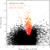 |
Fig. 1 MK versus WRP, BP−RP−WKS−KS < 4 colors of 2 MASS stars brighter than Ks − 1.311 × (H−Ks−02) < 8 mag and with good Gaia parallax. Selected cRSGs (in red and orange) lie in the cone enclosed by the two curves. The dotted cyan curve indicates a rough separation between O-rich AGB stars and C-rich AGB stars (to the right). The long-dashed red curve separates RSGs from O-rich AGBs and S-type stars. Stars included in the catalog of Messineo & Brown (2019) are colored in orange. |
2.1 Available photometry
The stars were selected from Gaia and 2MASS catalogs. The Two Micron All Sky Survey (2MASS) survey is described in Skrutskie et al. (2006), and in Cutri et al. (2003), and in the online manual4. The stars are extremely bright at infrared wavelength, and all measurements come from the 2MASS short-exposure frames (51 ms). The J-band measurements range from 1.89 to 8.68 mag, with a peak around 5 mag, while the H-band magnitudes range from 0.96 to 14.77 mag and peak at 3.5 mag, and the Ks magnitudes range from 0.66 to 7.70 mag with a peak at 3.0 mag. Stars that were saturated in the short integration frames had their profile reconstructed using the unsaturated pixels. While magnitudes of unsaturated point sources (fl_red=1) have a typical uncertainty of 0.01−0.02 mag, magnitudes of saturated sources (fl_red=3) are accurate within 0.2 mag. For 5% of the stars measurements from the Catalog of Infrared Observations (CIO) 5th edition by Gezari et al. (1996) are available; K measurements are available for all stars in the subsample: H mag for 44% and J mag for 22%. The average difference between the CIO and 2MASS J magnitudes brighter than 4 are +0.15 with a standard deviation σ=0.12 mag. Between the CIO and 2MASS H magnitudes brighter than 4, it is +0.24, with a standard deviation σ=0.44 mag; the average difference between the CIO and the 2MASS Ks magnitudes brighter than 4 is +0.00 mag, with a standard deviation of σ=0.62 mag; however, after excluding J03232718+6545417 and J08104310–1519469, the average difference becomes 0.07 mag with a σ of 0.17 mag.
Positional matches (within 5′′) in the Midcourse Space Experiment catalog (MSX, Egan et al. 2003) were found for 89% of the newly selected stars; 94% were found in the Wide-field Infrared Survey Explorer (WISE) survey (Wright et al. 2010), 25% were found in the Galactic Legacy Infrared Midplane Survey Extraordinaire (GLIMPSE) survey (Churchwell et al. 2009), and 26% were found in the MIPSGAL 24 μm survey (Gutermuth & Heyer 2015) using a search radius of 4′′.
JHKs measurements were all retained including 2MASS upper limits; however, a flag is given to indicate sources with the good 2MASS photometry. The SED of each star was visually inspected and a few measurements which appeared unrelated to the SED were removed. 2MASS J20434317+4741398, J17594120–2857418, and J14090677–5943243 had their H-band upper-limit magnitudes removed, 2MASS J18095816–2728222 had the WISE measurements removed (confusion and blend), 2MASS J18440043–0457062 had the WISE W3 and W4 magnitudes removed (confusion), 2MASS J10572371-6046304 had the WISE W4 upper limit magnitude removed, and 2MASS J19283960+1718220 had its GLIMPSE [3.6] magnitude removed (artifact on image).
2.2 Spectral types, temperatures, and extinction of cRSGs
In this work, a selection of cRSGs is presented. Although estimates of stellar parameters are provided, they are primarily used to ensure a good selection of stars. More accurate determinations of stellar parameters will require high-resolution spectroscopic follow-up observations and updated photometry.
The determination of Teff in RSGs is a challenging task. A direct determination of Teff requires the knowledge of the stellar radii, which are only available for a limited number of stars through interferometric measurements. More commonly, Teff values are estimated using color temperatures or spectroscopic temperatures (e.g., Levesque et al. 2005). Historically, the TiO bands visible in the optical spectra of RSGs have been used to determine their spectral types. By using models of stellar atmospheres (such as the MARCS models) and a fitting technique, Levesque et al. (2005) established a TiO-based temperature scale. However, as discussed in Davies et al. (2013), these models are far from perfectly reproducing observed spectra, and there is a degeneracy between extinction and temperature determination. Furthermore, both Davies et al. (2013) and Levesque (2018) demonstrated that the 1D MARCS models fail to accurately reproduce infrared fluxes, and using either the optical or infrared portion of the SED can result in different Teff values (and, consequently, extinction estimates).
These findings raise concerns about the use of TiO bands for determining Teff, leading to alternative attempts at temperature determination using atomic lines (see, e.g., Gazak et al. 2014; Tabernero et al. 2018; Dicenzo & Levesque 2019; Taniguchi et al. 2021, 2025). Messineo et al. (2021) show that the temperature measurements from Gazak et al. (2014) based on J-band spectra (R=11 000−14 000) agree with those of Levesque et al. (2005) to within 150 K. Tabernero et al. (2018) propose a new temperature scale based on spectral features in the CaT range (R=7000), confirming a correlation between TiO band depths and stellar temperatures. Taniguchi et al. (2025) determine RSG temperatures using YJ spectra (R=28 000) and 11 pairs of atomic iron lines; their temperatures are in good agreement with the Teff from TiO of Levesque et al. (2005) to within 100 K.
In conclusion, the use of TiO bands to determine temperatures remains valid, as it is supported by studies of atomic lines. Currently, spectroscopic temperatures can be used as a proxy for Teff, with a typical accuracy level of 100−150 K.
2.2.1 Spectral types
We analyzed the BPRP spectra to estimate KM types of the newly selected 342 O-rich stars. 327 BPRP spectra were available, but four were excluded because of poor quality, and four stars had spectra typical of G-types. Among the 15 stars without BPRP spectra, three do not have types in SIMBAD. In conclusion, a clean sample of 335 bright K- and M-type stars was produced.
The sample contains 135 previously unknown late-type stars, which we classified solely using the Gaia DR3 BPRP spectra. Because of a degeneracy between temperatures and reddening, an independent initial guess of interstellar extinction was required. Late-type stars span a small range of naked H−KS colors, and, initially, we assumed a fixed M1-type star with a naked H−Ks = 0.22 mag (Koornneef 1983) and an interstellar power law with an index of −2.1 (Messineo et al. 2005; Messineo 2024); because the associated color uncertainty is typically below 0.12 mag (the delta color between an M1 and an M5), we estimated an AKs uncertainty within 0.16 mag. The optical extinction curve by Cardelli et al. (1989), extrapolated to the near-infrared with a power law of index −2.1, was used to de-redden the BPRP spectra. Spectral types were inferred by matching the de-reddened BPRP spectra of the target stars with those of reference stars, as described in Messineo (2023). A few types were visually inferred if the solution diverged. The process was reiterated; with the obtained spectral types, temperatures were estimated using the temperature scale of Levesque et al. (2005), and the total AKs extinction values were recalculated with the color tables of Koornneef (1983). Then, spectral types were re-estimated with the new total AKs and the spectral library. On the second iteration, as spectral types had been estimated, the total AKs values were estimated from the J−Ks color excesses. The larger separation in wavelengths of the two filters ensures a more sensitive meter. Furthermore, the stars are very bright, and, generally, the fainter J magnitudes are of better quality than the H and Ks. The total AKs estimates from HKs have an average error of 0.34 mag, while the total AKs estimates from JKs have an average error of 0.11 mag. In Fig. 2, two examples of BPRP spectra are shown along with the selected reference spectrum at the target’s extinction. A comparison with the 3D dust map of Green et al. (2019) and our total AKs values was possible for 180 stars; after transforming the map E(B-V) values to AKs (Bay 19) = E(B−V) × 3.1 × 0.077 mag, a mean difference of 0.04 mag was measured with a sigma of 0.10 mag, as shown in Fig. 3. However, 3D Galactic extinction maps are made with a spatial resolution of several arcminutes; while our total AKs values were estimated with the infrared colors of the considered star. We retained our calculation of extinction. As explained in the following section, for most of the stars, the interstellar extinction AKs (int) can be approximated with the total stellar extinction AKs(tot) because the envelope optical depth is negligible.
Using the subsample of stars with spectral types in the literature, it was estimated that the accuracy of the inferred spectral types mostly fit within two spectral types. In Fig. 4, the distribution of spectral types appears to peak at M2–M3 types, as expected for RSGs (see Fig. 5 in Messineo & Brown 2019). The newly selected sample of 335 K – and M-type stars still includes variable stars. The histogram of stars with a trimmed_range_mag_g_fov larger than 0.3 mag is overplotted in red. The variables are the dominant population for M5-M9 types. When only considering stars in areas A or B of Messineo & Brown (2019), the final sample consists of 282 stars.
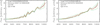 |
Fig. 2 Two examples of BPRP spectra. The target spectrum is shown with a black curve, and the reference spectrum with the dashed red curve. The reference spectrum was brought to the target’s extinction, which is estimated in the infrared. Extinction variations of ΔAKs = ± 0.05 mag and ± 0.10 are indicated with orange dotted and green dashed curves, respectively. Gaia source_ids are given in the figure labels. |
 |
Fig. 3 Left panel: estimated AKs (tot) values versus 3D dust map AKs (Bay 19) values. Center panel: AKs (tot)-AKs (env) values versus 3D dust map AKs (Bay 19) values. Right panel: for 16 stars with Teff < 3600 K and τ2.2 > 0.1, the AKs (tot) −AKs (env) values versus AKs (Mes24) values are plotted. |
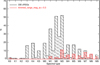 |
Fig. 4 Distribution of spectral types of 335 late-type stars analyzed. The histogram of stars with trimmed_range_mag_g_fov < 0.5 mag is shown in red. |
2.2.2 Envelop extinction
We assumed that the interstellar extinction AKs (int) can be accurately approximated by the total extinction AKs (tot) computed using the intrinsic colors of naked stars. The stars are by design the reddest in the WRP, BP−RP−WKS, J−KS color, as expected for early-M types, and their mass-loss rate is anticipated to be mild. The envelope optical depth of RSGs typically falls between 0.0 and 0.7 at 0.55 μm (Humphreys et al. 2020).
The optical depth of circumstellar envelopes can be measured by fitting infrared flux densities with DUSTY models. The mid-infrared features observed in the de-reddened stellar SED are intrinsically linked to the stellar envelope. Effective extinction ratios at mid-infrared wavelengths typically range from 0.3 to 0.5 times the value of AKS (Messineo 2024). These small variations in effective extinction ratios imply that, during the de-reddening process for interstellar extinction, the characteristics of these features remain consistent; an emission feature will consistently appear in emission, indicating an optically thin envelope. In summary, the envelope τ at 2.2 μm is estimated by examining the presence and strength of the silicate feature at 10 μm in the SED, alongside the flux excess at wavelengths longer than 8 μm.
A grid of SED models was constructed using the DUSTY algorithm of Ivezic et al. (1999). The NextGen spectra of Allard et al. (2011) with log10(g)=0.5, solar metallicity [M/H]=0 dex, and Teff from 2600 to 4500 K in steps of 100 K were utilized as input stellar models5. Cold silicates by Suh (1999) were used, and the optical depth at 2.2 μm, τ2.2, was varied in increments of 0.02 from 0 to 1.5. A maximum size of 1.000 μm and a minimum size of 0.001 μm were adopted for the Mathis–Rumpl–Nordsieck (MRN) size distribution. The most basic spherical envelope assumption was made with the density decreased as R−2 and a dust condensation radius at 1000 K. The temperature scale of Levesque et al. (2005) was used to translate the stellar spectral types (see the section above) to temperatures. After selecting the set of models that were closest to the stellar temperature, the τ2.2 was deduced by minimizing the discrepancies between the infrared observed fluxes (Fλ) and the model flux densities at the corresponding isophotal wavelengths. The theoretical SEDs obtained from synthetic spectra and the DUSTY radiative code were compared with the observed SEDs. When varying the stellar Teff of ± 100 K, the solution converged to the same τ2.2. While the majority of the observed SEDs are consistent with models of naked stars, some exhibit an emission feature around 10 μm accompanied by a flux excess beyond 8 μm6. Precisely, as seen in Fig. 5, the bulk of stars have negligible circumstellar extinction with τ2.2 < 0.02; for 7% of the sample, τ2.2 is larger than 0.25 (from 0.25 to 0.90), their SEDs show visible silicate features in emission, and a more accurate evaluation of interstellar extinction is needed.
The obtained τ2.2 is useful for relative comparisons of different envelope types. To compare this theoretical τ with the AKs (int) and AKs (tot) inferred from observations, we needed to scale the model τ to match the observed AKs (tot) −AKs (int). AKs (tot) is an equivalent total extinction because it is the total extinction obtained using the interstellar extinction law. The scaling parameters will depend on various factors, including the adopted grain composition (material and sizes), envelope geometry, and dust temperature. In this study, we assumed that the silicate models proposed by Suh (1999) are appropriate for the envelopes of cool cRSGs and will primarily explore the effect of the maximum grain size on the resulting τ.
An estimate of interstellar extinction, AKs (Bay 19), was obtained from maps (Green et al. 2019).
Another independent estimate of interstellar extinction, AKs (Mes24), was obtained with the technique outlined by Messineo (2024) for O-rich Mira stars. For mass-losing Miras, a fiducial sequence of intrinsic color-color points is adopted (e.g. in the plane (J−Ks)o vs. (Ks−[24])o), and used, along with the extinction-free color definition, to infer the interstellar extinction. For example,  − const × Ks−[24] = (J−Ks)o − const. ×(Ks−[24])o). By measuring
  , (J−Ks)o and (Ks−[24])o can be estimated; from the de-reddened (J−Ks)o and (Ks−[24])o, the interstellar AKs (Mes24) is estimated, as explained in Messineo (2024).
For 16 stars with DUSTY τ2.2 > 0.1 and Teff below 3600 K, budgeting of the interstellar extinction AKs (Bay 19) and AKs (Mes24), and the total extinction AKs (tot) was made. The AKs (int)=AKs(tot)-τ2.2 × factor, and the factor was chosen to avoid negative AKs(int)7. The AKs (int) values must be in agreement with the. AKs (Mes24) and AKs (Bay 19); we obtained that AKs (int) ≈AKs (tot)-τ2.2 × 0.3 (see Fig. 3), and the envelope extinction AKs (env) ≈0.3 × τ2.2 [0.001−1.000]. When the maximum gran size is 0.25−0.35 μm, the factor becomes unity; i.e., interstellar and circumstellar extinction curves become similar.
When neglecting the circumstellar envelope and assuming AKs (tot) as AK (int), the maximum overestimate of AK (int) would amount to 0.27 mag for the new sample. The correction AK(int)=AKs(tot)−AKs(env) was applied and the Mbol recalculated.
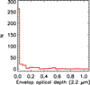 |
Fig. 5 Distribution of envelope optical depth at 2.2 μm of the newly selected late-type stars. |
2.3 Luminosities and bolometric corrections
One set of luminosities was obtained using the de-reddened 2MASS Ks, the Gaia distances of Bailer-Jones et al. (2021), the temperature scale, and the BCK of Levesque et al. (2005). The infrared extinction curve was approximated with a power law of index −2.1 (Messineo 2024). When changing the assumed spectral type of one unit (from M3 to M2 or M4), AKs varies by 0.03 mag on average (σ=0.01 mag), and the bolometric magnitudes Mbol(BCKs) change by 0.09 with sigma = 0.03 mag.
A second set of luminosities was derived with a trapezoidal integration under the SED made with the available infrared flux densities and by extrapolating to the blue side with the blackbody of the same temperature as the star, and to long wavelengths with a linear extrapolation to zero flux at 500 μm, as in Messineo & Brown (2019). The trapezoidal integration depends on the temperature through the blue extrapolation and extinction calculation. When changing the assumed spectral type of one unit (from M3 to M2 or M4), after recalculating AKs, the trapezoidal magnitudes change to 0.09 with sigma = 0.03 mag.
A third estimate of bolometric magnitudes (Mbol (DUSTY)) was obtained by integrating under the DUSTY model that best fit the observed infrared flux densities (de-reddened). The model was scaled so that the average of the observed JHKs flux densities best matched the average of the model flux densities at the isophotal wavelengths of the three 2MASS filters. The integrations were obtained in the plane Fν dν, the adopted zero-point constant was assumed to be −18.997, and the solar Mbol = +4.74 mag (Mamajek et al. 2015). The bin used for the τ2.2 grid corresponds to an Mbol uncertainty Mtauerr <0.01 mag, and the τ2.2 value remains unaffected by Teff variations within 100 K in the model. By shifting the best models of ± 100 K, Mbol variations are within 0.07 mag. When changing the assumed spectral type of one unit, after recalculating Teff and AKs, the Mbol (DUSTY) changes by 0.07 with sigma = 0.03 mag.
BCs for naked stars were derived with the NextGen models ([M/H]=0, log(g)=0.5) of Allard et al. (2011).
The dominant errors in Mbol come from the photometric uncertainties (±0.14 mag, when simultaneously decreasing or increasing the magnitudes by their errors) and the distance moduli (median errors are [+0.24,−0.27] mag, average errors are [+0.24,−0.27] with σ of [0.09,0.12] mag, see Table 1).
To calculate the global statistical errors on the three Mbol values, a Monte Carlo simulation was carried out (with 2001 runs). For each star, a table of 2001 Gaussian random errors was extracted for each available magnitude (using a different seed for each); each Gaussian had a 3 × σ equal to the quoted magnitude error. For each adopted spectral type, a Gaussian error with σ equal to two spectral types was randomly added. For each random extraction, magnitudes, spectral types, Teff, AKs, Mbol(BC), Mbol(trap), and Mbol(DUSTY) values were recalculated. The average magnitudes and σ values are given in Table 1.
The average difference between the Mbol values from the BCKS of Levesque et al. (2005) and those from the DUSTY models is −0.03 mag, with σ = 0.09 mag. The average difference between the trapezoidal Mbol values and those from the DUSTY model is −0.23 mag, with σ = 0.08 mag.
For the bulk of stars, the derived luminosities are consistent with those of RSGs, as shown in Fig. 6. They are mostly located in areas A and B of the luminosity-versus-temperature diagram.
The theoretical BCJ, BCH, and BCKS values estimated with the NextGen models ([M/H]=0, log(g)=0.5) of Allard et al. (2011) are listed in Table 2. The stellar temperature uncertainty affects the luminosity and the bolometric correction values. For the BC values of naked stars, uncertainties on the BC values depend on the slope of the relation between the BC values and the stellar Teff values, as explained by Levesque (2018) and shown in Fig. 7. The predicted slope in the Ks filter by Allard’s models is almost identical to that predicted with MARCS models by Levesque et al. (2005). The J band is particularly useful, because the gradient of the BC with increasing stellar temperature is negligible (for Teff > 3400 K). Differences in Teff corresponding to one nearby spectral type (e.g., from M0 to M1) amount to 45−85 K (Levesque et al. 2005). Therefore, a typical uncertainty in the Teff scale of 100−150 K (as noted in recent literature and described in Sect. 2.2) corresponds to two spectral subtypes (e.g., from M1 to M3). In the J band, for Teff from 3400 to 4500 K, an uncertainty of 100 K implies an uncertainty in BCJ of 0.015–0.035 mag, while in the Ks band, it implies an uncertainty in BCKS from 0.063 to 0.082 mag. However, the selection of the band must also take into account the effect of circumstellar extinction, which decreases with increasing wavelengths.
The presence of thick circumstellar envelopes changes the BC values, which can significantly deviate from those for naked stars (Messineo 2004; Davies et al. 2013; Messineo 2024). To understand the impact of envelope extinction on the Mbol values, the empirical bolometric correction in bands J, H, and Ks, BCJ, BCH, and BCKS values, were calculated as follows:
![Mathematical equation: $\begin{align*} & B C_{\mathrm{J}}=M_{{bol}}(\mathrm{DUSTY})-\left(\mathrm{J}-3.208 \times \mathrm{A}_{\mathrm{K}_{\mathrm{s}}}(\mathrm{int})-\mathrm{DM}\right)[\mathrm{mag}],\\ & B C_{\mathrm{H}}=M_{b o l}(\mathrm{DUSTY})-\left(\mathrm{H}-1.766 \times \mathrm{A}_{\mathrm{K}_{\mathrm{s}}}(\mathrm{int})-\mathrm{DM}\right)[\mathrm{mag}],\\ & B C_{\mathrm{K}_{\mathrm{S}}}=M_{{bol}}(\mathrm{DUSTY})-\left(\mathrm{K}_{\mathrm{S}}-\mathrm{A}_{\mathrm{K}_{\mathrm{s}}}(\mathrm{int})-\mathrm{DM}\right)[\mathrm{mag}], \end{align*}$](/articles/aa/full_html/2025/06/aa53900-25/aa53900-25-eq5.png)
where DM is the distance modulus, and J, H, and Ks are the 2MASS magnitudes. These empirical BCs are plotted versus the Teff values in Fig. 7. For Teff larger than 3300 K and τ2.2 < 0.08, the empirical BCJ values appear almost constant, with a mean value of 1.73 mag (σ = 0.05 mag) and a median value of 1.73 mag. In contrast, the theoretical BCJ has an average of 1.62 mag with a σ = 0.08 mag.
The empirical BCKS increases with decreasing temperature, but its slope is steeper than that derived from the theoretical models. At 3400 K, the BCKs is 0.07 mag larger than the theoretical value, while at 4100 K, it is 0.12 mag smaller than the theoretical value. The stars with visible infrared excess are marked and deviate from the relation for naked stars. Since for naked stars the BCJ values have little dependence on temperatures, the BCJ values clearly decrease with increasing AKs (env) in Fig. 8. When estimating the Mbol with the BCJ, one can underestimate the Mbol up to 0.6 mag.
The above description is based on Mbol values from synthetic spectra with solar metallicity. The theoretical dependence of the BCJ, BCH, and BCKs on the metallicity is also explored. In Fig. 9, the differences between BCs from models at [M/H]=+0.5 and those from models at [M/H]=+0.0 are displayed. For the NextGen models (panel a), Δ BCJ=0.05 mag with σ = 0.02 mag when considering Teff from 3200 to 4500 K; Δ BCH = −0.03 mag with σ = 0.01; and Δ BCKs = 0.014 mag with σ = 0.01. For the ATLAS9 models (panel b and d) the variations are: Δ BCJ = 0.050 mag with σ = 0.021 mag when considering Teff from 3200 to 4500 K; Δ BCH = −0.029 mag with σ = 0.006 mag; and Δ BCKs = −0.000 mag with σ = 0.006 mag. For the ATLAS9 models, similar differences are calculated when comparing models at [M/H]=+0.0 dex and models at [M/H]=−0.5 dex (which are not available in Allard’s NextGen grid).
In summary, uncertainties in BCs due to metallicity can be as high as 0.1 mag. Additionally, uncertainties in BCKs resulting from uncertain temperatures are of a similar magnitude (e.g., 0.12+0.08 mag for Teff=4100 K).
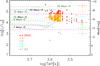 |
Fig. 6 Luminosities versus Teff of newly selected stars. Evolutionary tracks with solar metallicity and rotation by Ekström et al. (2012) are over-plotted. |
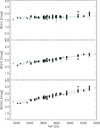 |
Fig. 7 Top panel: for stars with τ2.2 < 0.08, bolometric corrections BCJ are plotted versus Teff values with black-filled circles. For stars with τ2.2 > 0.08, gray crosses are plotted. The BC values were calculated with the Mbol inferred with the atmosphere models by Allard et al. (2011) and the DUSTY code and the absolute J magnitudes (from 2MASS). The dotted-dashed black line is the best polynomial fit of degree zero to the data points. The dashed green line is the theoretical BCJ inferred with Allard’s model ([M/H]=0, log(g)=0.5). The cyan squares mark the BCJ values estimated with an ATLAS9 grid of models and for Bessel filters by Howarth (2011) ([M/H]=0.0 and log(g)=0.5 dex); while our recalculations for the 2MASS filters are marked with red crosses. Middle panel: bolometric corrections BCH versus Teff values. Lines and symbols are as for the top panel. Bottom panel: bolometric corrections BCKs are plotted versus the Teff values. Lines and symbols are as for the top panel. The dashed-orange line is the K-band relation for naked RSGs found with MARCS models and the K-filter profile of Bessell & Brett (1988) by Levesque et al. (2005). |
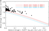 |
Fig. 8 Empirical BCJ values (Mbol(DUSTY) – (2 MASS.J − 3.208 × AKS(int) – DM)) are plotted versus inferred AK (env.). For supergiants (log(g)=0.5) of solar metallicity and Teff of 3200, 3900, and 4500 K, the theoretical BCJ calculated with the DUSTY simulation and Allard’s models are over-plotted. |
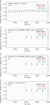 |
Fig. 9 Panel a: differences between BCs in J, H, and Ks bands inferred from the NextGen models of Allard et al. (2011) with log10(g)=0.5, [M/H]=0.5 dex, and Teff ranging from 2600 to 4500 K in steps of 100 K; and the BCs inferred from the same set of models, but with [M/H]=0.0 dex. Panel b: differences between BCs inferred from ATLAS9 models with log10(g)=0.5, [M/H]=0.5 dex, and Teff=3500, 3750, 4000, 4250, and 4500 K; and the BCs inferred from the same set of models, but with [M/H]=0.0 dex. Panel c: differences between BCs inferred from ATLAS9 models with log10(g)=0.5, [M/H]=0.0 dex, and Teff=3500, 3750, 4000, 4250, 4500 K; and the BCs inferred from the same set of models, but with [M/H]=−0.5 dex. Panel d: similar to Panel (b); this time, the ATLAS9 models are those distributed by Howarth (2011). Dotted horizontal lines are drawn every 0.1 mag for easier visualization. |
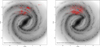 |
Fig. 10 Right panel: XY view of stars located in areas A and B of Mbol versus Teff diagram of Messineo & Brown (2019) and newly selected Gaia-2MASS cRSGs, which are also located in areas A and B (red dots). The background grayscale image is the artistic XY view of the Galactic plane illustrated by Dr. Hurt. Left panel: red data points show the complementary dataset (2122 stars with equal brightness (MK< −8.5 mag), which were excluded from the cRSGs). |
2.4 Isolation versus clustering
In the present work, we individually selected cRSGs on the basis of their color and luminosities. Due to their young age (5−40 Myr), RSGs are found to be associated with giant molecular complexes (e.g., Messineo et al. 2014a, 2021); however, at their ages, most of the stellar clusters have probably already been dissolved. They must therefore be detected individually, and the Gaia parallax allows us to do this.
Most of the efforts of the past two decades were focused on identifying clusters rich in RSGs. Until 2006, the only clusters known with four and five RSGs were Westerlund 1 and NGC 7419 (e.g., Clark et al. 2005; Caron et al. 2003). From 2006 to 2012, marvelous and rare stellar clusters rich in RSGs (RSGC1, RSGC2, RSGC3, Alicante7, Alicante8) were detected in the Milky Way between longitudes 25∘ and 35∘ at a heliocentric distance of about 6 kpc, located at the near end side of the Galactic bar (Figer et al. 2006; Davies et al. 2007; Clark et al. 2009b; Messineo et al. 2014b; Chun et al. 2024). The strict selection of parallax quality used in the present work excluded any member of these three distant clusters rich in RSGs located at the near-end side of the Galactic bar.
Eighteen percent of the newly selected cRSGs are found to be cluster members. Each stellar position was searched in VIZIER, and the appearing catalogs of cluster members were annotated. Then, the memberships were re-retrieved automatically by combining the matches found in the following catalogs: Cantat-Gaudin & Anders (2020), Castro-Ginard et al. (2022), Tarricq et al. (2022), Cantat-Gaudin et al. (2018), van Groeningen et al. (2023), Hunt & Reffert (2024), Kos (2024), Chi et al. (2023), Qin et al. (2023), He et al. (2023b), He et al. (2023a), He et al. (2022a), He et al. (2022b), Hao et al. (2022), Orellana et al. (2021), Dias et al. (2018), and Sampedro et al. (2017). If matches were found in multiple catalogs, only the first was retained (following the above listing) and only if the probability of membership was higher than 60%. All used catalogs, except for Sampedro et al. (2017), are based on Gaia data. The cluster membership is annotated in Table 1.
Theoretically, the precise age of a simple stellar population hosting RSGs depends on the inclusion and strength of stellar rotation. For non-rotating models, RSGs are found to populate clusters with ages from 4.5 to 40 Myr (e.g., Messineo et al. 2011). Observationally, small variations in age may arise from the selected sample of members and average parallax. Cluster parameters were taken from the compilation by Perren et al. (2023), as well as from the VIZIER database. For each cluster, the two most recent determinations of age and distance were collected. For 58% of cRSGs associated with a cluster, the cluster ages are consistent with the hosting of an RSG; i.e., they are younger than 41 Myr. For 40%, the associated clusters are older than 41 Myr; all but three cRSGs are younger than 300 Myr. The selection seems to yield ≈60% of authentic RSGs. When excluding members from the work of Sampedro et al. (2017), which is not based on Gaia parallaxes, this percentage rises to 66%.
A full investigation of the stellar clusters is beyond the scope of this paper. The names of the clusters and their ages are listed in the target list (Table 1).
3 XY distribution and longitude-velocity diagram
Asymptotic giant branch stars, being old, are good tracers of the Galactic potential, and, for example, their kinematics have been studied to characterize the central Galactic bar (e.g., Habing et al. 2006; Xia et al. 2024). On the contrary, RSGs are young and their distribution and kinematics give a picture of the Galactic locations where massive star formation occurred between 5 and 30−40 Myr ago; there is approximately one RSG for every burst of 10 000 stars (e.g., Clark et al. 2009a). That is, RSGs are young enough to still mark sites of violent cloud collisions and gas compression, and they populate the spiral arms. Galaxies are far from precise mathematical logarithmic spirals. Spiral arms are transitional phenomena, forms, and reforms. A closer look at the pictures of grand design spirals shows a richness of arms and connecting ridges. In the Milky Way, discussion is ongoing with regard to the actual number of spiral arms; it may be from two to four (Hou & Han 2014), or perhaps there are two that bifurcate.
In Fig. 10, the best sample of cRSGs, individually selected from Gaia, is overlaid on an artistic representation of the Galactic plane based on Spitzer data by Dr. Hurt8; yet, in Fig. 11 the sample of highly probable RSGs is plotted in the XY plane, in the longitude and latitude diagram, and in the velocity-versus-longitude diagram. We considered a sample of 762 bright late-type stars that are located in areas A and B of the luminosity-versus-Teff diagram and with radial velocity. 466 stars are from the literature collection by Messineo & Brown (2019)9, 20 are from Messineo (2023), and 276 are from the present work. For 96% of the sample, radial velocities were available in the main Gaia DR3 catalog (Katz et al. 2023). The remaining 4% of the measurements were found in the compilation of radial velocities by Tsantaki et al. (2022); this included a few measurements from APOGEE and Gaia DR2 velocities (not included in the Gaia DR3 release). The Gaia barycentric radial velocities were transformed in the local standard of rest (LSR) system using the solar motion by Reid et al. (model A5, 2019). In the XY plane of Fig. 11, the model of spiral arms made with distance measures of pulsars (Cordes & Lazio 2002) is superimposed.
The new selection adds stars at greater distances from us and deeper into the inner Galaxy to touch the Scutum-Centaurus arm. The distribution of cRSGs appears far from being homogeneous; indeed, there are several over-densities of cRSGs along the spiral arms, and filaments of cRSGs decorate the inter-arm regions. In Fig. 11, the large over-density on the Perseus spiral arm is colored in green (100∘ < l < 150∘, 1 < Y < 4 kpc). Another concentration of stars, colored cyan, appears on the Sagittarius arm at −55∘>l>−80∘ and 7.3 ≲ Y < 8.0 kpc; in the longitude-velocity diagram, this concentration appears to be stretched along the terminal velocity curve, and to end at the tangent point10 (as indicated in Table 2 of Hou & Han 2014) of the Sagittarius arm at l ≈−78∘, consistently with the arm modeling of Hou & Han (2014). A narrow feature, colored orange, is visible on the longitudes-versus-latitudes plot, showing decreasing latitudes with increasing longitudes (between −35∘ > l > −55∘ and −2∘ < b < 0∘). In the XY plane, this feature appears as a group of stars closer to the inner ScutumCentaurus arm (Y < 6.7 kpc). In the longitude-velocity diagram, these stars lie along the terminal velocity curve and culminate at the tangent point of the Scutum-Centaurus arm at l ≈−50∘ (e.g., Englmaier & Gerhard 1999; Hou & Han 2014). A filament of cRSGs appears aligned with the Local Arm, another filament extends from −5 < X < 0 kpc at Y ≈9 kpc.
Despite the small numbers, this appearance shows a remarkable resemblance with the distribution of giant molecular clouds (GMC) shown in the work of Hou & Han (2014). The cRSGs are not evenly distributed along the spiral arms, and they also populate the inter-arm regions. The two over-densities centered on the Perseus arm at l ≈ 130∘, and on the Sagittarius arm at l ≈−70∘ appear symmetrically disposed around the Sun along directions where over-densities of GMCs also lie (Hou & Han 2014).
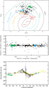 |
Fig. 11 Upper panel: XY view of cRSGs from areas A and B of Messineo & Brown (2019), along with new Gaia-2MASS cRSGs. A distance of 8.5 kpc is adopted, as in the work of Ocker & Cordes (2024). Green filled circles indicate stars located on the large over-density of RSGs of the Perseus arm. Cyan filled circles mark stars corresponding to an apparent concentration of RSGs at the tangent point of the Sagittarius-Carina arm at 1 ≈−78∘ (Hou & Han 2014). Orange-filled circles indicate stars located at the tangent point of the Scutum-Centaurus arm (at 1 ≈−50∘, Hou & Han 2014). Known massive clusters (>104 M⊙) rich in RSGs are marked in red. The spiral arms of Cordes & Lazio (2002), taken from the native NE2001p Python code of Ocker & Cordes (2024), are also shown. Middle panel: longitudes versus latitudes of cRSGs. The green, cyan, and orange data points are as specified in the upper panel. Lower panel: vLSR velocities versus longitudes of cRSGs (shown in yellow). The green, cyan, and orange data points are as specified in the upper panel. The background grayscale image is the CO map by Dame et al. (2001). Four points with peculiar velocities are indicated with pink diamonds; three of them are at high latitudes. |
4 Summary
An exercise to select bright late-type stars, cRSGs, from GAIA and 2MASS catalogs was carried out. While Messineo & Brown (2019) made a catalog of stars previously classified as class I cool stars, Messineo (2023) looked at the Gaia DR3 parameters to locate about 20 additional cRSGs and to find out that, for cool bright stars, the extinction and temperatures are still highly uncertain. The photometric diagnostics presented in Messineo (2023) were adopted here to select 335 additional cRSGs, with 282 located in areas A & B (39 in area A and 243 in area B). Only 12 of these stars are included in the catalog of Healy et al. (2024). Only six of the 335 stars have Gaia DR3 RVS data; however, they belong to areas E and C. There are no Gaia DR3 RVS data for stars in areas A and B, which is our conservative definition of cRSGs.
A small percentage (18%) of stars are found to be members of stellar clusters. While 58% of the clusters are reported to be younger than 41 Myr old, most have ages below 300 Myr. By extrapolating these percentages to the entire sample, 58% should be true RSGs.
In the XY plane, the cRSGs appear to follow the spiral arms and to populate inter-arm regions. The known Perseus over-density of RSGs is clearly visible. The velocity-longitude diagram suggests that two other over-densities of the XY plane are related to tangent points. A number of cRSGs appear to be aligned with the Local Arm.
Data availability
Gaia DR3 and 2MASS_Id provided in table1.dat, and Gaia BPRP spectra and 2MASS chartes are available at the CDS via anonymous ftp to cdsarc.cds.unistra.fr (130.79.128.5) or via https://cdsarc.cds.unistra.fr/viz-bin/cat/J/A+A/698/A282. Some chartes and spectra plots are displayed in https://mariamessineo.github.io/rsg_Ak/
Acknowledgements
This work has made use of data from the European Space Agency (ESA) mission Gaia (http://www.cosmos.esa.int/gaia), processed by the Gaia Data Processing and Analysis Consortium (DPAC, http://www.cosmos.esa.int/web/gaia/dpac/consortium). Funding for the DPAC has been provided by national institutions, in particular the institutions participating in the Gaia Multilateral Agreement. This publication makes use of data products from the Two Micron All Sky Survey, which is a joint project of the University of Massachusetts and the Infrared Processing and Analysis Center/California Institute of Technology, funded by the National Aeronautics and Space Administration and the National Science Foundation. This work is based on observations made with the Spitzer Space Telescope, which is operated by the Jet Propulsion Laboratory, California Institute of Technology under a contract with NASA. This research made use of data products from the Midcourse Space Experiment, the processing of which was funded by the Ballistic Missile Defense Organization with additional support from the NASA office of Space Science. This publication makes use of data products from WISE, which is a joint project of the University of California, Los Angeles, and the Jet Propulsion Laboratory/California Institute of Technology, funded by the National Aeronautics and Space Administration. This research has made use of the VizieR catalogue access tool, CDS, Strasbourg, France, and SIMBAD database. This research utilized the NASA’s Astrophysics Data System Bibliographic Services. We thank the Python, Astropy, NumPy, Pandas, Pivo, SciPy, Matplolib communities for providing their packages. We thank Dr. Hurt for his illustrations of the Milky Way. This work uses the RSG catalog by Messineo M. & Brown A. (2019) which was supported by the National Natural Science Foundation of China (NSFC-11773025, 11421303), and USTC grant KY2030000054. MM thanks Prof. Anthony Brown for helping her to realize the 2019 catalog, and Dr. Schuyler D. Van Dyk for appreciating her infrared catalog; this fact motivated this additional search for cRSGs. Another acknowledgment goes to Prof. Frank Bertoldi for discussion on interstellar extinction.
References
- Abia, C., de Laverny, P., Romero-Gómez, M., & Figueras, F., 2022, A&A, 664, A45 [NASA ADS] [CrossRef] [EDP Sciences] [Google Scholar]
- Allard, F., Homeier, D., & Freytag, B., 2011, in Astronomical Society of the Pacific Conference Series, 448, 16th Cambridge Workshop on Cool Stars, Stellar Systems, and the Sun, eds. C. Johns-Krull, M. K. Browning, & A. A. West, 91 [Google Scholar]
- Bailer-Jones, C. A. L., Rybizki, J., Fouesneau, M., Demleitner, M., & Andrae, R., 2021, AJ, 161, 147 [Google Scholar]
- Bayo, A., Rodrigo, C., Barrado Y Navascués, D., et al. 2008, A&A, 492, 277 [NASA ADS] [CrossRef] [EDP Sciences] [Google Scholar]
- Bessell, M. S., & Brett, J. M., 1988, PASP, 100, 1134 [Google Scholar]
- Cantat-Gaudin, T., & Anders, F., 2020, A&A, 633, A99 [NASA ADS] [CrossRef] [EDP Sciences] [Google Scholar]
- Cantat-Gaudin, T., Jordi, C., Vallenari, A., et al. 2018, A&A, 618, A93 [NASA ADS] [CrossRef] [EDP Sciences] [Google Scholar]
- Cardelli, J. A., Clayton, G. C., & Mathis, J. S., 1989, ApJ, 345, 245 [Google Scholar]
- Caron, G., Moffat, A. F. J., St-Louis, N., Wade, G. A., & Lester, J. B., 2003, AJ, 126, 1415 [Google Scholar]
- Castro-Ginard, A., Jordi, C., Luri, X., et al. 2022, A&A, 661, A118 [NASA ADS] [CrossRef] [EDP Sciences] [Google Scholar]
- Chi, H., Wang, F., Wang, W., Deng, H., & Li, Z., 2023, ApJS, 266, 36 [Google Scholar]
- Chun, S.-H., Myeong, G., Lee, J.-J., & Oh, H., 2024, AJ, 167, 230 [Google Scholar]
- Churchwell, E., Babler, B. L., Meade, M. R., et al. 2009, PASP, 121, 213 [Google Scholar]
- Clark, J. S., Negueruela, I., Crowther, P. A., & Goodwin, S. P., 2005, A&A, 434, 949 [NASA ADS] [CrossRef] [EDP Sciences] [Google Scholar]
- Clark, J. S., Davies, B., Najarro, F., et al. 2009a, A&A, 504, 429 [NASA ADS] [CrossRef] [EDP Sciences] [Google Scholar]
- Clark, J. S., Negueruela, I., Davies, B., et al. 2009b, A&A, 498, 109 [NASA ADS] [CrossRef] [EDP Sciences] [Google Scholar]
- Cordes, J. M., & Lazio, T. J. W., 2002, arXiv e-prints [arXiv:astro-ph/0207156] [Google Scholar]
- Cutri, R. M., Skrutskie, M. F., van Dyk, S., et al. 2003, 2MASS All Sky Catalog of point sources [Google Scholar]
- Dame, T. M., Hartmann, D., & Thaddeus, P., 2001, ApJ, 547, 792 [Google Scholar]
- Davies, B., Figer, D. F., Kudritzki, R.-P., et al. 2007, ApJ, 671, 781 [NASA ADS] [CrossRef] [Google Scholar]
- Davies, B., Kudritzki, R.-P., Plez, B., et al. 2013, ApJ, 767, 3 [Google Scholar]
- de Jong, R. S., Bellido-Tirado, O., Chiappini, C., et al. 2012, SPIE Conf. Ser., 8446, 84460T [Google Scholar]
- Dias, W. S., Monteiro, H., & Assafin, M., 2018, MNRAS, 478, 5184 [Google Scholar]
- Dicenzo, B., & Levesque, E. M., 2019, AJ, 157, 167 [NASA ADS] [CrossRef] [Google Scholar]
- Egan, M. P., Price, S. D., Kraemer, K. E., et al. 2003, VizieR Online Data Catalog: 5114 [Google Scholar]
- Ekström, S., Georgy, C., Eggenberger, P., et al. 2012, A&A, 537, A146 [Google Scholar]
- Englmaier, P., & Gerhard, O., 1999, MNRAS, 304, 512 [NASA ADS] [CrossRef] [Google Scholar]
- Figer, D. F., MacKenty, J. W., Robberto, M., et al. 2006, ApJ, 643, 1166 [Google Scholar]
- Gaia Collaboration (Vallenari, A., et al.,) 2023, A&A, 674, A1 [NASA ADS] [CrossRef] [EDP Sciences] [Google Scholar]
- Gazak, J. Z., Davies, B., Kudritzki, R., Bergemann, M., & Plez, B., 2014, ApJ, 788, 58 [NASA ADS] [CrossRef] [Google Scholar]
- Gehrz, R., 1989, in IAU Symposium, 135, Interstellar Dust, eds. L. J. Allamandola, & A. G. G. M. Tielens, 445 [Google Scholar]
- Gezari, D. Y., Pitts, P. S., Schmitz, M., & Mead, J. M., 1996, VizieR Online Data Catalog: 2209 [Google Scholar]
- Green, G. M., Schlafly, E., Zucker, C., Speagle, J. S., & Finkbeiner, D., 2019, ApJ, 887, 93 [NASA ADS] [CrossRef] [Google Scholar]
- Gutermuth, R. A., & Heyer, M., 2015, AJ, 149, 64 [Google Scholar]
- Habing, H. J., Sevenster, M. N., Messineo, M., van de Ven, G., & Kuijken, K., 2006, A&A, 458, 151 [NASA ADS] [CrossRef] [EDP Sciences] [Google Scholar]
- Hao, C. J., Xu, Y., Wu, Z. Y., et al. 2022, A&A, 660, A4 [NASA ADS] [CrossRef] [EDP Sciences] [Google Scholar]
- He, Z., Li, C., Zhong, J., et al. 2022a, ApJS, 260, 8 [NASA ADS] [CrossRef] [Google Scholar]
- He, Z., Wang, K., Luo, Y., et al. 2022b, ApJS, 262, 7 [NASA ADS] [CrossRef] [Google Scholar]
- He, Z., Liu, X., Luo, Y., Wang, K., & Jiang, Q. 2023a, ApJS, 264, 8 [NASA ADS] [CrossRef] [Google Scholar]
- He, Z., Luo, Y., Wang, K., et al. 2023b, ApJS, 267, 34 [Google Scholar]
- Healy, S., Horiuchi, S., Colomer Molla, M., et al. 2024, MNRAS, 529, 3630 [NASA ADS] [CrossRef] [Google Scholar]
- Hou, L. G., & Han, J. L., 2014, A&A, 569, A125 [NASA ADS] [CrossRef] [EDP Sciences] [Google Scholar]
- Howarth, I. D., 2011, MNRAS, 413, 1515 [NASA ADS] [CrossRef] [Google Scholar]
- Humphreys, R. M., Helmel, G., Jones, T. J., & Gordon, M. S., 2020, AJ, 160, 145 [NASA ADS] [CrossRef] [Google Scholar]
- Hunt, E. L., & Reffert, S., 2024, A&A, 686, A42 [NASA ADS] [CrossRef] [EDP Sciences] [Google Scholar]
- Ivezic, Z., Nenkova, M., & Elitzur, M., 1999, arXiv e-prints [arXiv:astro-ph/9910475] [Google Scholar]
- Katz, D., Sartoretti, P., Guerrier, A., et al. 2023, A&A, 674, A5 [NASA ADS] [CrossRef] [EDP Sciences] [Google Scholar]
- Koornneef, J., 1983, A&A, 128, 84 [NASA ADS] [Google Scholar]
- Kos, J., 2024, A&A, 691, A28 [NASA ADS] [CrossRef] [EDP Sciences] [Google Scholar]
- Levesque, E. M., 2018, ApJ, 867, 155 [Google Scholar]
- Levesque, E. M., Massey, P., Olsen, K. A. G., et al. 2005, ApJ, 628, 973 [Google Scholar]
- Limongi, M., 2017, in Handbook of Supernovae, eds. A. W. Alsabti, & P. Murdin, 513 [CrossRef] [Google Scholar]
- Maíz Apellániz, J., Pantaleoni González, M., & Barbá, R. H., 2021, A&A, 649, A13 [NASA ADS] [CrossRef] [EDP Sciences] [Google Scholar]
- Mamajek, E. E., Prsa, A., Torres, G., et al. 2015, arXiv e-prints [arXiv:1510.07674] [Google Scholar]
- Massey, P., Neugent, K. F., Dorn-Wallenstein, T. Z., et al. 2021a, ApJ, 922, 177 [NASA ADS] [CrossRef] [Google Scholar]
- Massey, P., Neugent, K. F., Levesque, E. M., Drout, M. R., & Courteau, S., 2021b, AJ, 161, 79 [NASA ADS] [CrossRef] [Google Scholar]
- Messineo, M., 2004, PhD thesis, University of Leiden, The Netherlands [Google Scholar]
- Messineo, M., 2023, A&A, 671, A148 [NASA ADS] [CrossRef] [EDP Sciences] [Google Scholar]
- Messineo, M., 2024, A&A, 686, A222 [NASA ADS] [CrossRef] [EDP Sciences] [Google Scholar]
- Messineo, M., & Brown, A. G. A., 2019, AJ, 158, 20 [NASA ADS] [CrossRef] [Google Scholar]
- Messineo, M., & Brown, A. G. A., 2021, https://doi.org/10.5281/zenodo.4964818 [Google Scholar]
- Messineo, M., Habing, H. J., Menten, K. M., et al. 2005, A&A, 435, 575 [NASA ADS] [CrossRef] [EDP Sciences] [Google Scholar]
- Messineo, M., Davies, B., Figer, D. F., et al. 2011, ApJ, 733, 41 [NASA ADS] [CrossRef] [Google Scholar]
- Messineo, M., Menten, K. M., Figer, D. F., et al. 2014a, A&A, 569, A20 [NASA ADS] [CrossRef] [EDP Sciences] [Google Scholar]
- Messineo, M., Zhu, Q., Ivanov, V. D., et al. 2014b, A&A, 571, A43 [NASA ADS] [CrossRef] [EDP Sciences] [Google Scholar]
- Messineo, M., Zhu, Q., Menten, K. M., et al. 2017, ApJ, 836, 65 [NASA ADS] [CrossRef] [Google Scholar]
- Messineo, M., Habing, H. J., Sjouwerman, L. O., Omont, A., & Menten, K. M., 2018, A&A, 619, A35 [NASA ADS] [CrossRef] [EDP Sciences] [Google Scholar]
- Messineo, M., Figer, D. F., Kudritzki, R.-P., et al. 2021, AJ, 162, 187 [NASA ADS] [CrossRef] [Google Scholar]
- Meynet, G., & Maeder, A., 2000, A&A, 361, 101 [NASA ADS] [Google Scholar]
- Ocker, S. K., & Cordes, J. M., 2024, RNAAS, 8, 17 [Google Scholar]
- Orellana, R. B., De Biasi, M. S., & Paíz, L. G., 2021, MNRAS, 502, 6080 [Google Scholar]
- Perren, G. I., Pera, M. S., Navone, H. D., & Vázquez, R. A., 2023, MNRAS, 526, 4107 [NASA ADS] [CrossRef] [Google Scholar]
- Qin, S., Zhong, J., Tang, T., & Chen, L., 2023, ApJS, 265, 12 [NASA ADS] [CrossRef] [Google Scholar]
- Reid, M. J., Menten, K. M., Brunthaler, A., et al. 2019, ApJ, 885, 131 [Google Scholar]
- Sampedro, L., Dias, W. S., Alfaro, E. J., Monteiro, H., & Molino, A., 2017, MNRAS, 470, 3937 [NASA ADS] [CrossRef] [Google Scholar]
- Sharma, S., Hayden, M. R., Bland-Hawthorn, J., et al. 2022, MNRAS, 510, 734 [Google Scholar]
- Skiff, B. A., 2014, VizieR Online Data Catalog: 1 [Google Scholar]
- Skrutskie, M. F., Cutri, R. M., Stiening, R., et al. 2006, AJ, 131, 1163 [NASA ADS] [CrossRef] [Google Scholar]
- Smith, N., & Tombleson, R., 2015, MNRAS, 447, 598 [NASA ADS] [CrossRef] [Google Scholar]
- Suh, K.-W., 1999, MNRAS, 304, 389 [NASA ADS] [CrossRef] [Google Scholar]
- Tabernero, H. M., Dorda, R., Negueruela, I., & González-Fernández, C., 2018, MNRAS, 476, 3106 [NASA ADS] [CrossRef] [Google Scholar]
- Taniguchi, D., Matsunaga, N., Jian, M., et al. 2021, MNRAS, 502, 4210 [NASA ADS] [CrossRef] [Google Scholar]
- Taniguchi, D., Matsunaga, N., Kobayashi, N., et al. 2025, A&A, 693, A163 [NASA ADS] [CrossRef] [EDP Sciences] [Google Scholar]
- Tarricq, Y., Soubiran, C., Casamiquela, L., et al. 2022, A&A, 659, A59 [NASA ADS] [CrossRef] [EDP Sciences] [Google Scholar]
- Tsantaki, M., Pancino, E., Marrese, P., et al. 2022, A&A, 659, A95 [NASA ADS] [CrossRef] [EDP Sciences] [Google Scholar]
- van Groeningen, M. G. J., Castro-Ginard, A., Brown, A. G. A., Casamiquela, L., & Jordi, C., 2023, A&A, 675, A68 [NASA ADS] [CrossRef] [EDP Sciences] [Google Scholar]
- Wright, E. L., Eisenhardt, P. R. M., Mainzer, A. K., et al. 2010, AJ, 140, 1868 [Google Scholar]
- Xia, T.-Y., Shen, J., Li, Z., et al. 2024, ApJ, 976, 139 [Google Scholar]
The catalog was revised to include Gaia eDR3 parallaxes (Messineo & Brown 2021; Messineo 2023).
The extinction calculation determines the exact number of stars in these regions.
As in Messineo & Brown (2019), Area A is defined as Mbol < − 7.1 mag, which is the AGB limit. Area B is coded as −7.1 < Mbol < −5.0 mag and L/L⊙>51.3−13.33 × log(Teff), with log(Teff[K]) > 3.548.
The spectra are distributed by the Virtual Observatory SED analyzer (Bayo et al. 2008). The bt-nextgen_agss2009 (gas only) were retrieved.
This simple approach (SED modeling) could not be used for AGBs by Messineo (2024) and Messineo et al. (2018) because the AGB Miras are strongly variable; by using non-simultaneously taken single-epoch measurements, their SEDs appeared as a zigzag without displaying a clear 10 μm feature.
DUSTY τ2.2 decreases with decreasing maximum grain size. τ2.2[0.001−1.000]=2.78 × τ2.2[0.001−0.350] and τ2.2[0.001− 1.000]=3.40 × τ2.2[0.001−0.250].
For homogeneity, the luminosities and areas of stars in Messineo & Brown (2019) and Messineo (2023) were re-estimated with the same extinction law adopted here; i.e., using an infrared extinction law with index =−2.1. They had previously been calculated with an index =−1.9.
“One can identify some of the dense emission ridges in the CO longitude-velocity diagram with Galactic spiral arms; where these meet the terminal velocity curve, they can be recognized as bumps where δ vt/δ l=0 … The inferred spiral arm tangents coincide with features along the terminal curve” (Englmaier & Gerhard 1999).
All Tables
BCs for naked stars were derived with the NextGen models ([M/H]=0, log(g)=0.5) of Allard et al. (2011).
All Figures
|
Fig. 1 MK versus WRP, BP−RP−WKS−KS < 4 colors of 2 MASS stars brighter than Ks − 1.311 × (H−Ks−02) < 8 mag and with good Gaia parallax. Selected cRSGs (in red and orange) lie in the cone enclosed by the two curves. The dotted cyan curve indicates a rough separation between O-rich AGB stars and C-rich AGB stars (to the right). The long-dashed red curve separates RSGs from O-rich AGBs and S-type stars. Stars included in the catalog of Messineo & Brown (2019) are colored in orange. |
| In the text | |
|
Fig. 2 Two examples of BPRP spectra. The target spectrum is shown with a black curve, and the reference spectrum with the dashed red curve. The reference spectrum was brought to the target’s extinction, which is estimated in the infrared. Extinction variations of ΔAKs = ± 0.05 mag and ± 0.10 are indicated with orange dotted and green dashed curves, respectively. Gaia source_ids are given in the figure labels. |
| In the text | |
|
Fig. 3 Left panel: estimated AKs (tot) values versus 3D dust map AKs (Bay 19) values. Center panel: AKs (tot)-AKs (env) values versus 3D dust map AKs (Bay 19) values. Right panel: for 16 stars with Teff < 3600 K and τ2.2 > 0.1, the AKs (tot) −AKs (env) values versus AKs (Mes24) values are plotted. |
| In the text | |
|
Fig. 4 Distribution of spectral types of 335 late-type stars analyzed. The histogram of stars with trimmed_range_mag_g_fov < 0.5 mag is shown in red. |
| In the text | |
|
Fig. 5 Distribution of envelope optical depth at 2.2 μm of the newly selected late-type stars. |
| In the text | |
|
Fig. 6 Luminosities versus Teff of newly selected stars. Evolutionary tracks with solar metallicity and rotation by Ekström et al. (2012) are over-plotted. |
| In the text | |
|
Fig. 7 Top panel: for stars with τ2.2 < 0.08, bolometric corrections BCJ are plotted versus Teff values with black-filled circles. For stars with τ2.2 > 0.08, gray crosses are plotted. The BC values were calculated with the Mbol inferred with the atmosphere models by Allard et al. (2011) and the DUSTY code and the absolute J magnitudes (from 2MASS). The dotted-dashed black line is the best polynomial fit of degree zero to the data points. The dashed green line is the theoretical BCJ inferred with Allard’s model ([M/H]=0, log(g)=0.5). The cyan squares mark the BCJ values estimated with an ATLAS9 grid of models and for Bessel filters by Howarth (2011) ([M/H]=0.0 and log(g)=0.5 dex); while our recalculations for the 2MASS filters are marked with red crosses. Middle panel: bolometric corrections BCH versus Teff values. Lines and symbols are as for the top panel. Bottom panel: bolometric corrections BCKs are plotted versus the Teff values. Lines and symbols are as for the top panel. The dashed-orange line is the K-band relation for naked RSGs found with MARCS models and the K-filter profile of Bessell & Brett (1988) by Levesque et al. (2005). |
| In the text | |
|
Fig. 8 Empirical BCJ values (Mbol(DUSTY) – (2 MASS.J − 3.208 × AKS(int) – DM)) are plotted versus inferred AK (env.). For supergiants (log(g)=0.5) of solar metallicity and Teff of 3200, 3900, and 4500 K, the theoretical BCJ calculated with the DUSTY simulation and Allard’s models are over-plotted. |
| In the text | |
|
Fig. 9 Panel a: differences between BCs in J, H, and Ks bands inferred from the NextGen models of Allard et al. (2011) with log10(g)=0.5, [M/H]=0.5 dex, and Teff ranging from 2600 to 4500 K in steps of 100 K; and the BCs inferred from the same set of models, but with [M/H]=0.0 dex. Panel b: differences between BCs inferred from ATLAS9 models with log10(g)=0.5, [M/H]=0.5 dex, and Teff=3500, 3750, 4000, 4250, and 4500 K; and the BCs inferred from the same set of models, but with [M/H]=0.0 dex. Panel c: differences between BCs inferred from ATLAS9 models with log10(g)=0.5, [M/H]=0.0 dex, and Teff=3500, 3750, 4000, 4250, 4500 K; and the BCs inferred from the same set of models, but with [M/H]=−0.5 dex. Panel d: similar to Panel (b); this time, the ATLAS9 models are those distributed by Howarth (2011). Dotted horizontal lines are drawn every 0.1 mag for easier visualization. |
| In the text | |
|
Fig. 10 Right panel: XY view of stars located in areas A and B of Mbol versus Teff diagram of Messineo & Brown (2019) and newly selected Gaia-2MASS cRSGs, which are also located in areas A and B (red dots). The background grayscale image is the artistic XY view of the Galactic plane illustrated by Dr. Hurt. Left panel: red data points show the complementary dataset (2122 stars with equal brightness (MK< −8.5 mag), which were excluded from the cRSGs). |
| In the text | |
|
Fig. 11 Upper panel: XY view of cRSGs from areas A and B of Messineo & Brown (2019), along with new Gaia-2MASS cRSGs. A distance of 8.5 kpc is adopted, as in the work of Ocker & Cordes (2024). Green filled circles indicate stars located on the large over-density of RSGs of the Perseus arm. Cyan filled circles mark stars corresponding to an apparent concentration of RSGs at the tangent point of the Sagittarius-Carina arm at 1 ≈−78∘ (Hou & Han 2014). Orange-filled circles indicate stars located at the tangent point of the Scutum-Centaurus arm (at 1 ≈−50∘, Hou & Han 2014). Known massive clusters (>104 M⊙) rich in RSGs are marked in red. The spiral arms of Cordes & Lazio (2002), taken from the native NE2001p Python code of Ocker & Cordes (2024), are also shown. Middle panel: longitudes versus latitudes of cRSGs. The green, cyan, and orange data points are as specified in the upper panel. Lower panel: vLSR velocities versus longitudes of cRSGs (shown in yellow). The green, cyan, and orange data points are as specified in the upper panel. The background grayscale image is the CO map by Dame et al. (2001). Four points with peculiar velocities are indicated with pink diamonds; three of them are at high latitudes. |
| In the text | |
Current usage metrics show cumulative count of Article Views (full-text article views including HTML views, PDF and ePub downloads, according to the available data) and Abstracts Views on Vision4Press platform.
Data correspond to usage on the plateform after 2015. The current usage metrics is available 48-96 hours after online publication and is updated daily on week days.
Initial download of the metrics may take a while.