| Issue |
A&A
Volume 698, June 2025
|
|
|---|---|---|
| Article Number | A110 | |
| Number of page(s) | 16 | |
| Section | Galactic structure, stellar clusters and populations | |
| DOI | https://doi.org/10.1051/0004-6361/202553729 | |
| Published online | 06 June 2025 | |
Origin of compressive turbulence in protoclumps in high redshift disks
1
Racah Institute of Physics, The Hebrew University,
Jerusalem
91904,
Israel
2
SCIPP, University of California,
Santa Cruz,
CA
95064,
USA
3
AIM, CEA, CNRS, Université Paris-Saclay, Université Paris Diderot, Sorbonne Paris Cité,
91191
Gif-sur-Yvette,
France
4
Departamento de Fisica Teorica, Modulo 8, Facultad de Ciencias, Universidad Autonoma de Madrid,
28049
Madrid,
Spain
5
CIAFF, Facultad de Ciencias, Universidad Autonoma de Madrid,
28049
Madrid,
Spain
6
Department of Physics, University of California,
Santa Cruz,
CA,
95064,
USA
★ Corresponding author: This email address is being protected from spambots. You need JavaScript enabled to view it.
Received:
12
January
2025
Accepted:
21
April
2025
Abstract
Context. The giant star-forming clumps in gas-rich high-redshift disks are commonly assumed to form due to gravitational instabilities, in which protoclumps have a Toomre-Q parameter less than unity. However, some cosmological simulations have shown that clumps can form in regions where Q is significantly greater than unity. In these simulations, there is an energy excess of compressive modes of turbulence that lead to gravitational collapse of regions that were not supposed to collapse under their own self-gravity, according to linear Toomre instability. In contrast, sites of clump formation in isolated simulations do not show this excess, suggesting that the origin of the compressive turbulence may be external.
Aims. We explore two external mechanisms that can induce the compressive modes of disk turbulence in protoclumps, namely, compressive tides exerted by the cosmological environment and the direct driving by inflowing streams.
Methods. We correlated the local strength of compressive tides and the amount of fresh stream material with protoclump regions in zoom-in cosmological simulations. We derived the local strength of compressive tides from the eigenvalues of the tidal tensor, and the local strength of incoming streams was derived from the fractional presence of the stream compared to the average.
Results. We find that the tidal field in protoclumps tends to be over-compressive, while random patches in the disk show substantial diverging tides. In particular, in 25% of the protoclumps, the tidal field is fully compressive, while no random patch resides in regions of fully compressive tides. In addition, the protoclumps tend to reside in regions where the fraction of the incoming stream mass is two to ten times larger than the average at the same galactocentric radius.
Conclusions. Both compressive tides and inflowing streams are correlated with the protoclumps and can thus serve as the drivers of the excessive compressive turbulence that can initiate clump formation before self-gravity takes over. This nature of turbulence constitutes a new non-linear mode of violent disk instabilities in high-z galaxies.
Key words: ISM: kinematics and dynamics / galaxies: evolution / galaxies: high-redshift / galaxies: ISM / galaxies: kinematics and dynamics
© The Authors 2025
 Open Access article, published by EDP Sciences, under the terms of the Creative Commons Attribution License (https://creativecommons.org/licenses/by/4.0), which permits unrestricted use, distribution, and reproduction in any medium, provided the original work is properly cited.
This article is published in open access under the Subscribe to Open model. This email address is being protected from spambots. You need JavaScript enabled to view it. to support open access publication.
1 Introduction
High-redshift galactic disks have been observed to be highly perturbed, sustain supersonic levels of turbulence (Hennebelle & Falgarone 2012; Kassin et al. 2012; Rowland et al. 2024), and host giant kiloparsec-scale clumps (Genzel et al. 2008; Guo et al. 2018; Zanella et al. 2019; Fujimoto et al. 2024). Approximately 40–60% of galaxies in the redshift range 1 ≤ z ≤ 4 appear to exhibit such clumpy structures (Guo et al. 2015; Shibuya et al. 2016). These clumps are prominent across various wavelengths, appearing in rest-frame UV (Wuyts et al. 2012; Guo et al. 2015; Sattari et al. 2023), Hα emission (Genzel et al. 2011; Swinbank et al. 2012; Livermore et al. 2015), CII (Zanella et al. 2024), and rest-frame optical and IR (Förster Schreiber et al. 2011; Kalita et al. 2024). They contribute roughly 10–20% of the galaxy’s total star formation rate (SFR), but their observed masses are more uncertain due to limited resolution (Cava et al. 2018; Meng & Gnedin 2020; Huertas-Company et al. 2020).
The presence of clumps in galactic disks significantly influences their structural and dynamical evolution. Clumps are believed to play a pivotal role in radial mass transport within the disk (Dekel et al. 2009; Dekel & Burkert 2014; Genzel et al. 2023; see also Dutta Chowdhury et al. 2024); in contributing to bulge growth (Zolotov et al. 2015; Lapiner et al. 2023); in creating cored dark matter halos through dynamical friction heating (Ogiya & Nagai 2022); and in driving turbulence via clump-clump and clump-disk interactions (Dekel et al. 2009; Krumholz & Burkert 2010). These processes are relevant if clumps persist long enough to participate in them. Clump longevity remains under debate, with some studies suggesting a substantial fraction of long-lived clumps (Mandelker et al. 2017) and others arguing for a prolonged clumpy phase composed of short-lived clumps (Oklopčić et al. 2017). Disk properties (such as the gas fraction) contribute to clump longevity (Renaud et al. 2024), but stellar and supernova feedback are likely the primary factors. Thus, clumps hold critical insights into feedback processes in galaxies (Mayer et al. 2016; Ceverino et al. 2023; Dekel et al. 2022; cf. Fensch & Bournaud 2020) and help constrain them.
Observationally, clump age gradients support the existence of long-lived clumps and their migration toward the galactic center (Shibuya et al. 2016; Guo et al. 2018). In Ginzburg et al. (2021), we applied deep learning techniques to identify clumps in star-forming galaxies from the CANDELS survey, and we classified them by longevity (short- or long-lived) based on cosmological simulations of clumpy galaxies (Mandelker et al. 2017). Our findings indicated that these galaxies host long-lived clumps that tend to migrate inward. Theoretically, analytical models of clump survival and migration suggest that clumps in gas-rich galaxies with stellar masses around M* ~ 109.3 M⊙ at z ~ 2 are likely to survive and migrate, typically reaching the center within roughly ten clump free-fall times (Dekel et al. 2022). Cosmological simulations, however, present a more complex picture. While the VELA3 simulations (Ceverino et al. 2014; Zolotov et al. 2015; Mandelker et al. 2017) have clearly indicated the presence of long-lived clumps, the VELA6 simulations (Ceverino et al. 2023) as well as the FIRE simulations (Oklopčić et al. 2017) predominantly show short-lived clumps. The FIRE simulations typically exhibit outflow mass-loading factors ![Mathematical equation: $\[\eta \equiv \dot{M}_{\text {out}} / \mathrm{SFR} \sim 4{-}10\]$](/articles/aa/full_html/2025/06/aa53729-25/aa53729-25-eq1.png) and outflow velocities of 400–700 km s−1 (Muratov et al. 2015) in the relevant mass and redshift range. In contrast, for massive long-lived clumps in VELA (as seen in Fig. 13 of Mandelker et al. 2017), the mass-loading factor is around unity or less. This mass-loading factor is consistent with the observational estimate for ionized gas outflows driven by stellar and supernova feedback (Förster Schreiber et al. 2019).
and outflow velocities of 400–700 km s−1 (Muratov et al. 2015) in the relevant mass and redshift range. In contrast, for massive long-lived clumps in VELA (as seen in Fig. 13 of Mandelker et al. 2017), the mass-loading factor is around unity or less. This mass-loading factor is consistent with the observational estimate for ionized gas outflows driven by stellar and supernova feedback (Förster Schreiber et al. 2019).
While the giant clumps could have formed ex situ, being the remnants of small galaxies that merged with the disk, it is believed that most clumps formed in situ, due to local gravitational collapse. The common understanding of in situ clump formation is that they arise from violent disk instability governed by the Toomre instability (Toomre 1964). In this picture, a razor-thin disk becomes linearly unstable to axisymmetric perturbations when Q ≡ κσ/πGΣ < 1. Here, κ is the epicyclic frequency, σ is the radial velocity dispersion (either thermal or turbulent), and Σ is the surface density. While it is convenient and quite common to evaluate the Q parameter using global values of the disk, the Q parameter is derived locally at each galactocentric radius by assuming the scales of the perturbations are much smaller than the disk scale radius (Binney & Tremaine 2008). When taking the disk’s thickness into account, Romeo & Falstad (2013), following Romeo (1994), derived an order of unity correction factor to the two-dimensional Q parameter that depends on the anisotropy of the turbulence velocity field. The correction factor increases the Q parameter, which has a stabilizing effect on the disk. An increased Q parameter is equivalent to a decreased threshold for stability, to a typical value of ~0.68 for thick galactic disks (Goldreich & Lynden-Bell 1965).
Disks are typically assumed to be in a state of “marginal instability”, sustaining Q ~ Qcrit, where 0.68 ≲ Qcrit ≲ 2 (see below) the threshold for instability. This is based on the following qualitative argument (Noguchi 1999; Dekel et al. 2009): if a disk’s Q drops below Qcrit, the disk starts to fragment into rings in the linear regime, which later fragment non-linearly into filaments and feathers (Arora et al. 2025) and eventually collapse into bound clumps, thus developing non-axisymmetric features in the disk. Star formation within these clumps induces strong stellar feedback, and torques caused by the non-axisymmetric features drive angular momentum outward and thus drive mass inward, which flows down the potential well toward a central bulge. Both stellar feedback and radial mass transport are sources of turbulence (Krumholz et al. 2018), which raises the velocity dispersion and consequently Q above Qcrit. When Q grows above Qcrit, the disk stabilizes, clumps and non-axisymmetric features diminish, and turbulence-driving mechanisms weaken, allowing σ to decrease and Q to eventually fall below Qcrit again. While other drivers of turbulence – both internal and external of the disk – such as magnetorotational instabilities, spiral shocks, and external accretion (Federrath et al. 2017; Federrath 2018; Ginzburg et al. 2022) may play important roles at different masses and redshifts and should be incorporated into the picture in a self-consistent manner, this qualitative argument hints at a cyclical regulation mechanism that maintains the disk in a state of marginal stability, with Q ~ Qcrit. This was confirmed in numerical simulations of isolated disks (Immeli et al. 2004; Bournaud & Elmegreen 2009; Hopkins et al. 2012; Arora et al. 2025) as well as observations (Genzel et al. 2014; Fisher et al. 2017). However, caution should be taken when measuring Q in observations, especially in clumps, because these measurements are usually dominated by the high surface density non-linear structures, where Q is no longer meaningful.
In a cosmological setting, however, the situation is more complex. Inoue et al. (2016) showed that in the VELA simulations, clumps are formed out of “protoclump” regions, where the local two-component Q parameter (i.e., the Q parameter of a disk composed of stars and gas; (Rafikov 2001; Romeo & Wiegert 2011) is greater than an order of unity Qcrit and occasionally substantially greater. This calls into question the validity of the local linear Toomre analysis in cosmological disks. Several other formation mechanisms for clumps are possible. For example, Inoue & Yoshida (2018) have suggested a two-stage formation of clumps beginning with the development of spiral arms when Q ~ 2, followed by the fragmentation of these arms to clumps when Q ~ 0.6. However, this does not explain the clump formation in regions with Q > 3 in VELA. Another possibility is the rapid dissipation of turbulence in perturbed regions. Elmegreen (2011) showed that if significant energy dissipation occurs within a crossing time, the threshold for stability increases to Qcrit ~ 2–3, but this is again insufficient to explain the clump formation found by Inoue et al. (2016). Lovelace & Hohlfeld (1978) derived a necessary condition for non-axisymmetric perturbations to be unstable based on the existence of a local extremum of f(r) = ΣΩ/κ2. Some galaxies in the VELA simulations did show such a local extremum (Inoue et al. 2016), so it is possible that some clumps are formed due to non-axisymmetric perturbations. Other theories (e.g., Griv & Gedalin 2012) eventually boil down to a stability criterion of Qcrit ≳ 2.
In Mandelker et al. (2025) (henceforth M25), we initiated the exploration of the possibility that clumps form out of protoclump regions with high levels of compressive turbulence. Broadly speaking, the turbulence velocity field can be thought of as being composed of a compressive part, representing the local tendency to converge to or diverge from a point, and a solenoidal part, representing the local tendency to rotate about a point (see Kritsuk et al. 2007; Federrath et al. 2010, for an extensive and rigorous overview). These parts are represented by the divergence and curl of the velocity field, respectively (see Sect. 2.3). While cosmological simulations such as the ones used in M25 typically do not properly resolve the turbulence cascade, very high resolution isolated simulations do show a proper cascade of such motions (Bournaud et al. 2010; Fensch et al. 2023). For an isotropic and homogeneous turbulent field in equipartition, the global ratio of energy in compressive modes to total turbulent energy is ~1/3. However, if for any reason there is a deviation from this value in favor of compressive modes, the turbulence itself is able to generate more dense regions (Padoan & Nordlund 2002; Federrath et al. 2010), which can be sufficient for self-gravity to take over while having large velocity dispersions that keep Q above unity. Indeed, Hopkins & Christiansen (2013) found that, statistically, Q parameters of ≳51 are marginally stable in highly supersonic disks.
While inspecting both cosmological and isolated simulations, M25 found that protoclump regions in cosmological simulations do show an excess of energy in compressive modes, while protoclump regions in isolated simulations do not. This implies that the cosmological environment drives more compressive turbulence by physical processes that are absent in an isolated setting. In this work, we examine two possible causes for the excess of compressive modes of turbulence in a cosmological environment: compressive gravitational tides (a scenario in which Q may be altered; Jog 2014) and stream-disk interaction. For the former, several studies have shown that during galaxy mergers of other strong interactions, elevated levels of compressive tides induce clump and cluster formations as well as high levels of compressive turbulence (Renaud et al. 2009, 2014, 2022; Li et al. 2022). Mergers can also induce clump formation by the wake they produce during the merger (Nakazato et al. 2024). As for stream-disk interaction, it has the potential to drive turbulence due to the collision between the stream and the disk (see discussion in Sect. 4.2).
The paper is organized as follows. In Sect. 2, we introduce the methods used in our analysis, including turbulence decomposition (Sect. 2.3), tidal field analysis (Sect. 2.4), and stream-disk interaction analysis (Sect. 2.5). In Sect. 3, we present our main analysis, and in Sect. 3.2, we present a comparison of the fraction of energy in compressive modes, the tides, and the presence of streams between protoclumps and random patches, and in Sect. 3.3, we correlate the different quantities. In Sect. 4, we discuss some caveats, and in Sect. 5, we present our conclusions.
2 Methods
2.1 The VELA cosmological simulations
We analyze eight galaxies from the VELA3 suite of cosmological simulations2 (Ceverino et al. 2014; Mandelker et al. 2017). The simulations use the ART code (Kravtsov et al. 1997; Ceverino & Klypin 2009), which is a gravito-hydrodynamics, grid-based, adaptive mesh refinement code, with a maximal resolution of ~17–35 proper pc at all times, down to z ~ 1. The dark matter mass resolution is 8.3 · 104 M⊙, and the minimal stellar particle mass is 103 M⊙. The code includes gas and metal cooling, UV-background photoionization and self shielding in dense gas, stochastic star-formation, thermal feedback, radiation pressure and metal enrichment from stellar feedback (Ceverino et al. 2010, 2012, 2014). A more detailed description of the simulations can be found in Ceverino et al. (2014) and Mandelker et al. (2017). We use the high temporal resolution version of the simulations, which has ~30 snapshots per disk orbital time.
All of the eight galaxies undergo a phase of compaction to a blue nugget (sometimes multiple; Zolotov et al. 2015; Lapiner et al. 2023), which involves a rapid increase in the central gas density, followed by an intense starburst and subsequent inside-out quenching. These compaction events are usually triggered by a major merger (Lapiner et al. 2023), although not exclusively. The galactic disk survives for long periods of time when the halo mass exceeds ~1011 M⊙ (Dekel et al. 2020), which typically occurs after the compaction event. Thus, the main violent, disky3 phase of the galaxies typically lasts from z ~ 4 − 1 (Mandelker et al. 2017; Dekel et al. 2022), which is roughly the period of time analyzed in Inoue et al. (2016) and M25.
2.2 Clump finder and protoclumps
We use the clump finder developed by Mandelker et al. (2017). In short, the 3D density field of baryons is dumped onto a uniform grid with grid spacing of Δx = 70 pc. The grid is then smoothed with a spherical Gaussian with full-width-at-half-maximum of W = 2.5 kpc. The residual, δ, is then defined as δ = (ρ − ρW)/ρ, where ρ and ρW are the raw and smoothed density fields, respectively. Clumps are defined as connected regions containing at least eight uni-grid cells with δ > 10, as defined using either stellar density, or the combined density of cold gas (T < 1.5 · 104 K) and young stars (stellar age < 100 Myr).
Since VELA uses ART, which is a grid-based code, and the current run did not include tracer particles, clumps are tracked through time based on their stellar particles. We only tracked clumps that contain at least ten stellar particles, and for each clump at a given snapshot, we searched for all clumps in the previous snapshot that contribute at least 25% of their stellar particles to the current clump. If a given clump has more than one such progenitor, we considered the most massive one as the main progenitor and the others as having merged with it. We derived the formation time of the clump based on the snapshot at which no progenitor was found in the two preceding snapshots. The clumps in VELA were studied in detail in Mandelker et al. (2017), and their properties are consistent with properties of observed clumps (Guo et al. 2018; Ginzburg et al. 2021).
To define protoclump regions, that is, the regions out of which clumps form, we take the center-of-mass velocity of the clump at its initial formation snapshot in cylindrical coordinates (vr, vϕ, vz), and extrapolate the position one snapshot back in time to determine the position of the protoclump. Assuming that the clump has just formed, and given the high temporal resolution, it is safe to assume that the clump’s velocity is still attached to the overall disk velocity field. For the size of the protoclumps, since most of the collapsed clumps have radii in the range RC ~ 100–300pc (Mandelker et al. 2017), and clumps usually contract by a factor of two to three (Ceverino et al. 2012; Dekel et al. 2023), we use a fixed radius of RPC = 0.5 kpc for all protoclumps. We performed all of our analysis for RPC = 0.8 kpc with no qualitative difference.
2.3 Turbulence decomposition
The heart of our analysis is based on compressive turbulence. Compressible turbulence in general, and compressive turbulence in particular4 has been shown to impact the density distribution of interstellar gas (Federrath et al. 2010), which in turn affects star formation in regions with excess of compressive turbulence. Indeed, an extensive study by Federrath & Klessen (2012) demonstrated, analytically and numerically, that the star formation rates, as well as the star formation efficiencies, increase by orders of magnitude when the turbulence driving is dominated by compressive modes.
While compressive turbulence is conceptually simple to understand, it is mathematically more challenging to define. Below, we give two definitions, one local and one global, each having advantages but also drawbacks that present a caveat in our analysis. Discussion of these caveats is present in Sect. 4.3.
A word on terminology – we call the mode of turbulence that describes a tendency to locally diverge or converge to a point the “compressive mode”, and the mode of turbulence that describes a tendency to locally rotate about a point the “solenoidal mode”. Out of the two possible directions of the compressive mode, we have the “converging mode”, for which ∇ · v < 0, and the “diverging mode”, for which ∇ · v > 0.
2.3.1 Global decomposition
Every vector field v(r) can be decomposed, using the Helmholtz decomposition, to curl-free, divergence-free, and harmonic components:
![Mathematical equation: $\[\boldsymbol{v}(\boldsymbol{r})=\nabla \phi+\nabla \times \boldsymbol{A}+\nabla \psi \equiv \boldsymbol{v}_{\text {comp }}+\boldsymbol{v}_{\text {sol }}+\boldsymbol{v}_{\text {har }},\]$](/articles/aa/full_html/2025/06/aa53729-25/aa53729-25-eq2.png) (1)
(1)
where ϕ, ψ are scalar functions, with ψ satisfying ∇2ψ = 0 and A is a vector function. In order to perform this decomposition, appropriate boundary conditions are needed. Two types boundary conditions are commonly assumed, which make the decomposition straightforward – vanishing at infinity or periodic – both of which are not applicable in the local case. For the former, v → 0 as |r| → ∞, then necessarily ψ = const since ψ solves Laplace’s equation with ∇ ψ = 0 at the boundary5. The value of ψ is not physically important, only its gradient, which is zero. For the latter type of boundary condition, in a periodic box, ψ = 0 since a harmonic function cannot be periodic in every direction, and if v is periodic, ∇ ψ must be periodic, and hence ψ must be periodic.
In either of these cases, a periodic box or an infinite domain where v → 0 as |r| → ∞, the decomposition can be performed using the Fourier transform. This is achieved by projecting the Fourier transform of the velocity field along the wave vector k and perpendicular to k,
![Mathematical equation: $\[G_\phi(\boldsymbol{k})=\frac{i \boldsymbol{k} \cdot \tilde{\boldsymbol{v}}}{|\boldsymbol{k}|^2}, \quad \boldsymbol{G}_A(\boldsymbol{k})=\frac{i \boldsymbol{k} \times \tilde{\boldsymbol{v}}}{|\boldsymbol{k}|^2}.\]$](/articles/aa/full_html/2025/06/aa53729-25/aa53729-25-eq3.png)
Here, ![Mathematical equation: $\[\tilde{\boldsymbol{v}}\]$](/articles/aa/full_html/2025/06/aa53729-25/aa53729-25-eq4.png) is the Fourier transform of v. Using these two functions, we can write the Fourier transform of v as
is the Fourier transform of v. Using these two functions, we can write the Fourier transform of v as
![Mathematical equation: $\[\tilde{\boldsymbol{v}}=-i\boldsymbol{k} G_\phi+i \boldsymbol{k} \times \boldsymbol{G}_A.\]$](/articles/aa/full_html/2025/06/aa53729-25/aa53729-25-eq5.png) (2)
(2)
The desired curl-free and divergence-free parts are determined by the inverse Fourier transform of the above two terms. It is evident from this decomposition that ∇ · vcomp = ∇ · v and ∇ × vsol = ∇ × v.
From Parseval’s theorem, one finds that vcomp and vsol are orthogonal in the global sense,
![Mathematical equation: $\[\int|\boldsymbol{v}|^2 d^3 \boldsymbol{r}=\int\left|\boldsymbol{v}_{\text {comp }}\right|^2 d^3 \boldsymbol{r}+\int\left|\boldsymbol{v}_{\text {sol }}\right|^2 d^3 \boldsymbol{r},\]$](/articles/aa/full_html/2025/06/aa53729-25/aa53729-25-eq6.png) (3)
(3)
but not in a local sense (i.e., vcomp · vsol ≠ 0). This can easily be understood from the uncertainty principle – the decomposition is locally orthogonal in k-space, and therefore only globally orthogonal in r-space6. Another caveat with this decomposition is that it is possible to construct a velocity field such that at a given point, r0, v (r0) = 0, while vcomp (r0), vsol (r0) ≠ 0. Thus, assuming that |vcomp|2 and |vsol|2 represent some local energy densities in a region, even if relatively isolated, can introduce significant errors.
Nevertheless, we can use this decomposition to robustly define the global fraction of energy in compressive modes of turbulence (see also Federrath et al. 2010; Brunt & Federrath 2014), that is,
![Mathematical equation: $\[f_{\text {comp,glob }}=\frac{\int\left|v_{\text {comp }}\right|^2 d^3 \boldsymbol{r}}{\int|v|^2 d^3 \boldsymbol{r}}.\]$](/articles/aa/full_html/2025/06/aa53729-25/aa53729-25-eq7.png) (4)
(4)
While it can be analytically proven, it is intuitive to understand that in a fully isotropic and homogeneous turbulence7 in equipartition, fcomp,glob = 1/3 – converging or diverging to or from a point is a one dimensional radial motion, while rotation (characterized by the solenoidal mode) about a point is two dimensional. Furthermore, for a fully isotropic and homogeneous turbulence in equipartition, the converging mode is half the total compressive power.
2.3.2 Local decomposition
Given the inherit non-locality of the Helmholtz decomposition, a different method is required to characterize the compressiveness of the turbulence field on small, protoclump scales. The most common approach is based on the following.
If v(r) is the velocity at the center of the clump, r, then one can estimate the turbulence velocity field in the vicinity of this point is δv ≡ v(r + δr) − v(r). Since protoclumps are only mild overdensities, and tend to rotate with the disk, the variation of the velocity field within them can be interpreted as turbulence on scales smaller than the protoclump. This filtering approach is a common mathematical approximation for the turbulence field when one cannot resolve all the relevant scales (Schmidt et al. 2006; Garnier et al. 2009; Aluie 2013; Schmidt 2014; Semenov 2024), and methods stemming from this formalism have been applied to analyze turbulence in the context of disk instability in various galaxy simulations (Agertz et al. 2009a,b; Bournaud et al. 2014; Inoue et al. 2016; Goldbaum et al. 2015; Renaud et al. 2021; Ejdetjärn et al. 2022). Technically, this approach captures random motions about the local mean motion. A more formal approach requires detailed power spectrum analysis to show this obeys proper energy cascade. It is quite challenging to properly capture the energy cascade in numerical simulations, even in the relatively high resolution in our simulations (e.g., Kritsuk et al. 2011; Federrath et al. 2021; Semenov 2024); however, detailed analyses have shown that such a filtering approach properly captures the interaction between scales (Semenov 2024). We do note that very high resolution simulations of isolated galaxies do show that disk galaxies exhibit proper turbulence cascade (Bournaud et al. 2010; Fensch et al. 2023). While not properly resolved here, the converging flows in our simulations are somewhere along the beginning of the inertial range.
To a linear order, δv can be approximated as
![Mathematical equation: $\[\delta \boldsymbol{v}=\boldsymbol{v}(\boldsymbol{r}+\delta \boldsymbol{r})-\boldsymbol{v}(\boldsymbol{r}) \approx \frac{1}{3}(\boldsymbol{\nabla} \cdot \boldsymbol{v}) \delta \boldsymbol{r}+\frac{1}{2} \boldsymbol{\omega} \times \delta \boldsymbol{r}+\overleftrightarrow{S} \delta \boldsymbol{r},\]$](/articles/aa/full_html/2025/06/aa53729-25/aa53729-25-eq8.png) (5)
(5)
where ω = ∇ × v is the vorticity, and ![Mathematical equation: $\[\overleftrightarrow{S}\]$](/articles/aa/full_html/2025/06/aa53729-25/aa53729-25-eq9.png) is a traceless symmetric tensor representing shearing motion. While the second and third terms in Eq. (5) are orthogonal, the shear term is, in general, not orthogonal to either of them. This raises a complication in interpreting each component individually as a contributor to the total energy in the turbulence field.
is a traceless symmetric tensor representing shearing motion. While the second and third terms in Eq. (5) are orthogonal, the shear term is, in general, not orthogonal to either of them. This raises a complication in interpreting each component individually as a contributor to the total energy in the turbulence field.
As mentioned above, the deviation of the velocity field from the local mean rotation is interpreted as the turbulence velocity field. However, ∇ · v and ∇ × v properly capture this turbulent behavior even if the mean rotation is not subtracted, as long as it varies on scales larger than the scale of the protoclump8.
Other works tend to neglect the shearing term (Kida & Orszag 1990; Kritsuk et al. 2007; Renaud et al. 2014), and then the total turbulent kinetic energy in a sphere of radius R is
![Mathematical equation: $\[E_K \approx \frac{1}{9}(\nabla \cdot \boldsymbol{v})^2 \int r^4 d^3 \boldsymbol{r}+\frac{1}{4}|\nabla \times \boldsymbol{v}|^2 \int r^4 \sin ^2 \theta d^3 \boldsymbol{r},\]$](/articles/aa/full_html/2025/06/aa53729-25/aa53729-25-eq10.png) (6)
(6)
where the factor of sin2 θ comes from the cross product between ω and r. After integrating, we obtained
![Mathematical equation: $\[E_K \approx \frac{4 \pi}{9} \frac{R^5}{5}(\nabla \cdot \boldsymbol{v})^2+\frac{2 \pi}{3}|\nabla \times \boldsymbol{v}|^2 \frac{R^5}{5}.\]$](/articles/aa/full_html/2025/06/aa53729-25/aa53729-25-eq11.png) (7)
(7)
This motivates defining |∇ · v|2 as the local energy in compressive modes9, and |∇ × v|2 as the local energy in solenoidal modes10. We take the same approach, and discuss its caveats and potential future directions in Sect. 4.3. We thus defined the local fraction of energy in converging mode at a given point as
![Mathematical equation: $\[f_{\mathrm{conv}, \mathrm{loc}}=\frac{|\boldsymbol{\nabla} \cdot \boldsymbol{v}|_{\mathrm{neg}}^2}{|\boldsymbol{\nabla} \cdot \boldsymbol{v}|^2+|\boldsymbol{\nabla} \times \boldsymbol{v}|^2},\]$](/articles/aa/full_html/2025/06/aa53729-25/aa53729-25-eq12.png) (8)
(8)
where ![Mathematical equation: $\[|\boldsymbol{\nabla} \cdot \boldsymbol{v}|_{\text {neg }}^{2}\]$](/articles/aa/full_html/2025/06/aa53729-25/aa53729-25-eq13.png) refers to regions with negative divergence, representing compression (as opposed to expansion). As discussed in the Introduction and shown by turbulence box simulations (Federrath et al. 2010; Semenov 2024), an increasingly negative divergence leads to a larger turbulence velocity dispersion and, in particular, compressive turbulence, which promotes dense regions that can become self-gravitating. For a given region, the total fraction of energy in converging modes is thus
refers to regions with negative divergence, representing compression (as opposed to expansion). As discussed in the Introduction and shown by turbulence box simulations (Federrath et al. 2010; Semenov 2024), an increasingly negative divergence leads to a larger turbulence velocity dispersion and, in particular, compressive turbulence, which promotes dense regions that can become self-gravitating. For a given region, the total fraction of energy in converging modes is thus
![Mathematical equation: $\[f_{\mathrm{conv}}=\frac{\int|\boldsymbol{\nabla} \cdot \boldsymbol{v}|_{\mathrm{neg}}^2 d^3 \boldsymbol{r}}{\int|\boldsymbol{\nabla} \cdot \boldsymbol{v}|^2 d^3 \boldsymbol{r}+\int|\boldsymbol{\nabla} \times \boldsymbol{v}|^2 d^3 \boldsymbol{r}}.\]$](/articles/aa/full_html/2025/06/aa53729-25/aa53729-25-eq14.png) (9)
(9)
In Appendix A, we show that for a turbulent field in which the power spectrum of vcomp and vsol are proportional, with the appropriate boundary conditions, and when integrating over the entire volume,
![Mathematical equation: $\[\frac{\int\left|v_{\text {comp }}\right|^2 d^3 \boldsymbol{r}}{\int|v|^2 d^3 \boldsymbol{r}}=\frac{\int|\nabla \cdot \boldsymbol{v}|^2 d^3 \boldsymbol{r}}{\int|\nabla \cdot \boldsymbol{v}|^2 d^3 \boldsymbol{r}+\int|\boldsymbol{\nabla} \times \boldsymbol{v}|^2 d^3 \boldsymbol{r}}.\]$](/articles/aa/full_html/2025/06/aa53729-25/aa53729-25-eq15.png) (10)
(10)
Thus, the definitions of Eqs. (9) and (4) agree, contingent on the appropriate boundary conditions.
To calculate the local fraction in our simulations, we follow the method of M25. First, we dump our AMR grid onto a uniform grid with 0.2 kpc resolution. Then, we compute the nine derivatives of the velocity field, ∂vi/∂rj, using a second order, centered finite differences method. Then, for a given region, we integrate over its volume the quantities ![Mathematical equation: $\[|\boldsymbol{\nabla} \cdot \boldsymbol{v}|_{\text {neg }}^{2}\]$](/articles/aa/full_html/2025/06/aa53729-25/aa53729-25-eq16.png) (taking into account only cells with negative divergence), |∇ · v|2 and |∇ × v|2. We then define fconv of a given region, according to Equation (9). As discussed in Sect. 2.3.1, a value of 1/3 for the total power in compressive turbulence (compression or expansion) is expected in fully isotropic and homogeneous turbulence in equipartition, and thus a value of 1/6 is expected for fconv. While the turbulence in galactic disk is not necessarily isotropic and homogeneous (certainly not on scales larger than the scale height, where the turbulence becomes two-dimensional), we use these values as a reference, saying that regions with fconv > 0.33 have excess of converging modes.
(taking into account only cells with negative divergence), |∇ · v|2 and |∇ × v|2. We then define fconv of a given region, according to Equation (9). As discussed in Sect. 2.3.1, a value of 1/3 for the total power in compressive turbulence (compression or expansion) is expected in fully isotropic and homogeneous turbulence in equipartition, and thus a value of 1/6 is expected for fconv. While the turbulence in galactic disk is not necessarily isotropic and homogeneous (certainly not on scales larger than the scale height, where the turbulence becomes two-dimensional), we use these values as a reference, saying that regions with fconv > 0.33 have excess of converging modes.
We note that after the protoclump has collapsed to a clump it is expected to become rotation-supported, as shown in Ceverino et al. (2012), and thus fstr will go down.
2.4 Tidal field
When an extended body resides in a gravitational field, different mass elements experience slightly different gravitational forces. In the rest frame of the body, this difference translates to compression or expansion along different directions. The tidal field is in general not isotropic, and can be compressive or expansive in different directions. In principle, it can be fully compressive (i.e., compressive in every direction), but not fully expansive (see below).
Fully compressive tides can arise in systems which reside in cosmological environments (Renaud et al. 2009), but can also arise internally in isolated systems, even in smooth density profiles (Dekel et al. 2003). If a patch of the disk resides in a region where the tidal field is fully compressive, the turbulence in this region can become dominated by compression (Renaud et al. 2014), and this region may undergo a gravitational collapse due to the tides, eventually forming a giant clump. Mathematically, the tidal field is quantified by the tidal tensor, to be explained next.
The first order approximation for the gravitational acceleration about a point r0 is
![Mathematical equation: $\[F_j\left(\boldsymbol{r}_0+\delta \boldsymbol{r}\right)=F_j\left(\boldsymbol{r}_0\right)+\frac{\partial F_j}{\partial r_i} \delta r_i+\ldots,\]$](/articles/aa/full_html/2025/06/aa53729-25/aa53729-25-eq17.png) (11)
(11)
where we employ the summation notation. If ϕ(r) is the gravitational potential, then Fj = −∂ϕ/∂rj, and we can rewrite the acceleration, to a first order, as
![Mathematical equation: $\[F_j\left(\boldsymbol{r}_0+\delta \boldsymbol{r}\right) \approx-\left.\frac{\partial \phi}{\partial r_j}\right|_{\boldsymbol{r}_0}-\left.\frac{\partial^2 \phi}{\partial r_i \partial r_j}\right|_{\boldsymbol{r}_0} \delta r_i.\]$](/articles/aa/full_html/2025/06/aa53729-25/aa53729-25-eq18.png) (12)
(12)
We defined the tidal tensor as Tij = ∂2ϕ/∂ri∂rj. Under this definition, the first order approximation for the gravitational acceleration is
![Mathematical equation: $\[F_j\left(\boldsymbol{r}_0+\delta \boldsymbol{r}\right) \approx F_j\left(\boldsymbol{r}_0\right)-T_{i j} \delta r_i.\]$](/articles/aa/full_html/2025/06/aa53729-25/aa53729-25-eq19.png) (13)
(13)
The tidal tensor is a symmetric tensor, and therefore its eigenvectors are orthogonal, which means we can find an orthogonal basis that diagonalizes Tij. The eigenvalues are real, and we order them by value λ1 ≥ λ2 ≥ λ3. Using our definition, a positive eigenvalue represents compression along the direction of its corresponding eigenvector, while a negative value represents expansion along this direction11. If all eigenvalues are positive, the tidal field is said to be fully compressive. Since λ1 + λ2 + λ3 = trace(T) = ∇2ϕ = 4πGρ ≥ 0, λ1 is necessarily positive (i.e., the tidal field cannot be fully expansive), while λ2, λ3 can be either positive or negative.
Previous studies quantified the compressiveness of the tidal field solely by the third eigenvalue, λ3 (Renaud et al. 2009; Li et al. 2022). However, this approach is quite conservative, as while λ3 might be negative, λ1 and λ2 can simultaneously be positive, meaning that the tidal compression along their corresponding directions can be substantial. We therefore took a different approach and defined a quantity, ftides, that takes into account all eigenvalues, as follows. Assume a spherical region of size R and a constant density. As stated above, the tidal tensor is symmetric, and therefore we can align the coordinate system with its three eigenvectors. The mean value of the acceleration along the radial direction (indicative of compression/expansion) is then
![Mathematical equation: $\[\begin{aligned}F_t & =-\frac{1}{4 \pi / 3 R^3} \int(\overleftrightarrow{T} \boldsymbol{r}) \cdot \frac{\boldsymbol{r}}{r} d^3 \boldsymbol{r}=-\frac{1}{4 \pi / 3 R^3} \int T_{i j} r_j \frac{r_i}{r} d^3 \boldsymbol{r} \\& =-\frac{1}{4 \pi / 3 R^3} \int \frac{\lambda_1 x^2+\lambda_2 y^2+\lambda_3 z^2}{r} d^3 \boldsymbol{r}=-\frac{1}{4} R\left(\lambda_1+\lambda_2+\lambda_3\right) \\& \equiv-\frac{1}{4} R \lambda_1\left(1+f_{\text {tides }}\right),\end{aligned}\]$](/articles/aa/full_html/2025/06/aa53729-25/aa53729-25-eq20.png)
where we define
![Mathematical equation: $\[f_{\mathrm{tides}}=\frac{\lambda_2+\lambda_3}{\lambda_1}.\]$](/articles/aa/full_html/2025/06/aa53729-25/aa53729-25-eq21.png) (14)
(14)
This simple calculation motivates us to use ftides as a quantification of how compressive or expansive the tidal field is in a given spherical region – if ftides > 0, then the tidal field is substantially compressive along at least two directions (those of λ1 and λ2), and potentially fully compressive. If ftides < 0, at least along one direction (that of λ3), and potentially two directions (those of λ2 and λ3), the tidal field is substantially expansive12. As an example, for a spherically symmetric density profile, ftides = 2 − α(r), where α(r) is the logarithmic slope of the average density within r (Dekel et al. 2003). For values of α = 0, 1, 2, 3, corresponding to a flat core, a cuspy profile, an isothermal sphere and a point mass, respectively, ftides = 2, 1, 0, −1. Indeed, for a cored profile and a cuspy profile, the average tidal field is compressive. For a cored profile it is fully compressive in all three directions, while for a cuspy profile it is zero along the radial direction and compressive along the other two directions. For an isothermal sphere, the tidal field along the radial direction is expansive and equal in magnitude to the force along the other two directions, which are compressive. The average tidal force is thus zero. Finally, for a point mass, the tidal force along the radial direction is the strongest, and is expansive. After the protoclump collapses, it will dominate the potential in its vicinity, and thus ftides loses its ability to quantify tides induced by the larger environment of the galaxy.
To calculate the compressiveness of the tidal field in a particular region in our simulations, we first dump the gravitational potential onto the same grid uniform grid as in Sect. 2.3.2, and calculate the Hessian matrix using a second order, central finite differences method. Given that the resolution of the simulation in the regions of interest is ~20–100 pc, a grid of resolution of 0.2 kpc is sufficient to be well above the effective gravitational softening induced by the Poisson solver. We did perform similar analysis on a 0.4 kpc resolution grid, and found no qualitative differences. We then diagonalize the matrix at every grid cell (using the known analytical equations for 3 × 3 matrices) to get the three eigenvalues for each cell. Finally, we perform a volume-weighted average of each eigenvalue inside the given region, and plug the values into the definition of Eq. (14), to get ftides for each region of interest.
2.5 Stream-disk interaction
When the streams interact with the disk, intense shocks are expected to occur due to the collision of the stream material with the disk material, and turbulence is expected to be stirred (Ginzburg et al. 2022), especially if the streams are dense and clumpy due to fragmentation (Klessen & Hennebelle 2010; Forbes et al. 2023). Indeed, an ongoing series of papers, studying the evolution of cold streams feeding massive halos, has revealed that streams are expected to fragment into dense clumps, either gravitationally (Mandelker et al. 2018; Aung et al. 2019), or due to cooling (Mandelker et al. 2020; Aung et al. 2024). Furthermore, since the streams flow toward the central galaxy in the potential of the dark matter halo, gravitational focusing tends to make the streams narrower and denser as they reach the disk (Aung et al. 2024). Thus, we expect regions of the disk that interact with streams to be sites of high compressive turbulence that can lead to clump formation. This was briefly discussed in M25, and can be seen in Figure 3 therein. The degree to which stream-disk interaction drives turbulence is a subject of an ongoing work (Ginzburg et al. 2022, Ginzburg et al., in prep).
In the current work, we want to understand whether or not protoclump regions are also sites of stream-disk interaction, and how the local fraction of compressive turbulence in these regions differs from other regions in the disk that do not interact with streams. The VELA simulations are AMR hydro simulations that do not have tracer particles. It is therefore difficult to determine whether a mass element was recently brought by accretion or has been part of the disk for a long time. We therefore use the approximate streamline method developed by Dutta Chowdhury et al. (2024). In short, by assuming that the gas velocity field is roughly constant over a disk dynamical time, gas cells in a given snapshot can be traced using the gas velocity data of that snapshot only. Starting from its current 3D position, a gas cell in a given snapshot is traced back in time along its streamline to yield an approximate initial 3D position one dynamical time ago. If the distance between the initial and current positions is larger than 10% the disk radius, we tag this cell as a stream material. We refer the reader to Dutta Chowdhury et al. (2024) for a more elaborate description of the method.
To quantify whether or not a given protoclump region resides in a site where a stream is interacting with the disk, we look at an annulus at the same radius of the protoclump, with its width being the size of the protoclump, namely ΔR = 2RPC = 1 kpc. We then divide the annulus to angular bins of angular opening Δθ = dPC/rPC, where dPC = 1 kpc is the diameter of the protoclump region, and rPC is the distance of the protoclump region from the galactic center. We then defined
![Mathematical equation: $\[f_{\text {str }}=\frac{M_{\text {stream, PC}}}{\left\langle M_{\text {stream, slice}}\right\rangle},\]$](/articles/aa/full_html/2025/06/aa53729-25/aa53729-25-eq22.png) (15)
(15)
where Mstream,PC is the total mass of stream material in the protoclump’s angular bin, and ⟨Mstream,slice⟩ is the average stream mass in all angular bins within the annulus. In Figure 1 we show contours of fstr at 8 kpc from V07 at z ~ 2 and from V08 at z ~ 1. One can see the stream from the top left joining the disk, resulting in an increased fstr where the stream joins the disk.
After the clump forms, it is either quickly disrupted by feedback or lives for a long time (Mandelker et al. 2017; Dekel et al. 2023) and migrates to the center (Dekel et al. 2022). In the latter case, this will mean that fstr will go down as the clump migrates.
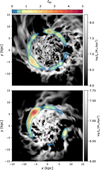 |
Fig. 1 Proof of concept for fstr. The background color shows the projected surface density of gas in V07 at z ~ 2 (top) and in V08 at z ~ 1 (bottom). The contours are of fstr in angular bins at a radius of 8 kpc in both panels. One can see how fstr increases in regions where the stream interacts with the disk. |
3 Results
We want to test whether or not protoclump regions form in regions with fully compressive tides and/or in sites of stream-disk interaction. Furthermore, we would like to quantify the fraction of energy in compressive modes in such regions, and in converging modes in particular, and compare to the excess in converging modes found in protoclump regions in M25. In order to differentiate protoclumps from the underlying disk, we associated each protoclump with a random patch that has the same distance from the galactic center and is of the same size as the protoclump region, making sure it does not overlap with other protoclump regions. In the following analysis, we analyze protoclumps corresponding to clumps with a maximal baryonic mass larger than 108 M⊙, similar to M 25. We calculate fconv, ftides and fstr as defined in Eqs. (9), (14) and (15) for the protoclump regions and the random patches in the disk, as outlined at the end of Sect. 2.3.2, Sect. 2.4 and Sect. 2.5.
In Sect. 3.1 we analyze the global fraction in compressive modes as a function of time. In Sect. 3.2 we compare the various quantities between protoclumps and their corresponding random patches, and in Sect. 3.3 we correlate the different quantities against the fconv.
3.1 Global fraction of compressive turbulence
In Figure 2, we show the fraction of turbulent energy in converging or compressive (converging plus diverging) modes, averaged over the whole disk, as defined in Eq. (10), as a function of the cosmological scale factor. We show the evolution of three out of the eight galaxies we analyze. One can see that, most of the time, the total fraction of energy in the compressive mode is about 1/3 (blue curve), as expected in fully isotropic and homogeneous turbulence in equipartition (see Sect. 2.3.1). The red curve shows only the fraction in converging modes, that is, only for cells with negative divergence. One can see that for V26 it is close to 1/6, while for V07 it is usually around 0.3. For V08, at early times, the total fraction of energy in converging modes is around 1/6, increasing to 1/3 at later times.
Each of these galaxies undergoes a compaction event that leads to a blue nugget (Zolotov et al. 2015), which is usually preceded by a major merger (Lapiner et al. 2023). One can see that before the major mergers and the subsequent compaction events occur, the fraction of energy in compressive modes (converging plus diverging) is roughly 1/3, as expected in a fully isotropic and homoegeneous turbulence in equipartition13. During the merger, one can see a sharp increase in the fraction of energy in global compression, similar behavior as seen in idealized simulations of galactic mergers (Renaud et al. 2014). As we show below in Sect. 3.2.2 and Figure 5, we find that clump formation is indeed correlated with compressive tides, which are expected to arise during mergers.
Overall, we strengthen the result of M25 that globally, the turbulence field does not deviate much from the equilibrium ratios, except when undergoing major mergers and compaction events.
3.2 Protoclumps versus random patches
We now turn to the local analysis in small regions in the disk. We start by comparing fconv, ftides and fstr between protoclump regions and random patches (as explained in the beginning of this section).
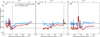 |
Fig. 2 Temporal evolution of the global fraction of turbulent energy in converging and diverging flows (blue curve) and in only converging (i.e., only cells with ∇ · v < 0; red curve) flows for three galaxies from our suite. The vertical black line indicates the moment of the blue nugget phase in each galaxy (Lapiner et al. 2023). The horizontal solid (dashed) lines indicate one third (sixth) of the total energy, values expected for fully isotropic and homogeneous turbulence in equipartition. Each of the blue nugget phases are preceded by at least one major merger, which increases the global fraction in compressive turbulence, before settling back to the equilibrium values. |
3.2.1 Compressive turbulence
In Figure 3 we show examples of snapshots from V07 and V08 at redshifts z ~ 2 and 1, respectively. The small black (magenta) circle in the left (right) panel marks a protoclump region. One can see that the two protoclump regions presented in Figure 3 reside in a part of the disk that interacts with a stream that comes from the top left corner (see also Figure 1). As we have argued above, this interaction can stir up turbulence, and can induce compression by local shocks which boosts the fraction of energy in converging modes, as clearly seen in the right panel of Figure 3, which shows the mass weighted projection of fconv. The same protoclump regions show elevated levels of converging modes of turbulence. Figure 3 shows other regions in the disk that have high values of fconv. While some of these may be other protoclumps, perhaps of clumps that were not identified by the clump finder, most of these regions are not dense enough to initiate gravitational collapse, or are susceptible to shear (as discussed in Sect. 4.3).
In Figure 4, we show the distribution of fconv in all protoclump regions and their corresponding random patches, for all of the eight galaxies. We can clearly see that fconv has very different distributions in protoclumps and random patches protoclump regions have a median fconv ~ 0.5, larger than the expected equilibrium value, while random patches have a median of fconv ~ 0.21, which is more in line with the expected equilibrium value of ~0.16. These results strengthen our results from M25, in which the analysis was performed only on V07.
3.2.2 Tides
In the left panel of Figure 5, we show the distribution of ftides in protoclump regions and random patches. Recall from Sect. 2.4 that a positive value of ftides is indicative of a substantial or fully compressive tidal field, while a negative value hints at substantial stripping along some direction. Figure 5 clearly shows that ftides has different distributions among protoclumps and random patches. While random patches have a median ftides ~ −0.26, protoclump regions have a median ftides ~0.32, with the vast majority of protoclumps having ftides > 0.
In the right panel of Figure 5, we show the distribution of λ3 (arbitrarily scaled, see caption) in protoclump regions and random patches. Although the distribution is of log λ3, negative values on the x-axis represent negative values of λ3 rather than values 0 < λ3 < 1 Gyr−1 (see caption). One can see that the tidal field in ~25% of the protoclumps is fully compressive, since λ3 > 0 and therefore all of the eigenvalues of the tidal tensor are positive. On the other hand all of the random patches have λ3 < 0, meaning that the tidal field is expansive along at least one direction. While this may hint that a consequence of clump formation is local, fully compressive gravitational tides, we remind the reader that the protoclump regions are mild, non-self gravitating (with Q ≫ 1; Inoue et al. 2016), local overdensities. Thus, it is unlikely that the cause for the compressive tides is due to the clump formation process, but rather due to sources external to the protoclump. A detailed study of the source of gravitational tides is needed to make this distinction (see discussion in Sect. 4.1).
We conclude from Figure 5 that almost all of the protoclumps reside in regions where the tidal field is substantially compressive, and almost exclusively, regions with fully compressive tides are protoclumps.
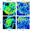 |
Fig. 3 Correlation of fconv with gas density in protoclump regions. In the left panels, we show the projected surface density of the gas. The top row represents V07 at z ~ 2, while the bottom row represents V08 at z ~ 1, as in Figure 1. The black circles indicate the location of a protoclump region. The white circle is the disk radius, defined as the radius that contains 85% of the cold gas in the disk. In the right panels, we show maps of mass weighted projections of fconv in the same snapshot. The small magenta circle shows the location of the same protoclump region, while the large magenta circle is the disk radius. One can see that inside the region of the protoclump, most of the mass has fconv ~0.5–0.8. Furthermore, we observed that the protoclump regions are close to where the stream joins the disk (see Sect. 2.5 and Figure 1). |
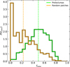 |
Fig. 4 Probability distribution of fconv in protoclump regions (green histogram) and random patches (orange histogram) over all eight galaxies. The vertical lines of each color indicate the median of the corresponding distribution. One can see that protoclump regions have a median fconv ~ 0.5, while random patches have a median fconv ~ 0.21, meaning that protoclump regions have a strong excess in converging modes compared to random patches in the disk, which are more in agreement with equilibrium values. |
3.2.3 Stream-disk interaction
In Figure 6, we show the distribution of fstr in protoclump regions and in their corresponding random patches. Random patches have, on average, fstr ~ 0.8, meaning that the stream mass in their vicinity is slightly less than the average over the annulus. For protoclump regions, we find on average fstr ~ 2.5, with a broad tail reaching fstr ~10, that is some protoclump regions have ten times more stream material than the average at their galactocentric radius, indicating that they reside in a site of stream-disk interaction.
The distributions of fstr in protoclumps and random patches are more similar than they are for both fconv and ftides, as can be seen by comparing Figures 4 and 5 (left panel) to Figure 6. However, recall that a major caveat in our defintion of fstr is the crude definition of stream material compared to disk material, due to the lack of tracer particles in our simulations (Dutta Chowdhury et al. 2024). Furthermore, an energy-based or momentum-based quantity would perhaps be more appropriate than the mass-based quantity we use here. However, without tracer particles, these quantities suffer similar uncertainties. Nevertheless, we find that fstr = 1 is around the 30th percentile of the distribution for protoclump regions, meaning that around 70% of the protoclumps reside in sites of stream-disk interaction, compared to only ~40% of random patches.
3.3 ftides and fstr versus fconv
In the previous section, we have found that protoclump regions tend to reside in regions where the turbulent velocity field is locally compressive (Sect. 3.2.1), tides are substantially or fully compressive (Sect. 3.2.2), and are sites of stream-disk interaction (Sect. 3.2.3). We now attempt to answer the question whether the tides or the stream-disk interactions cause the excess compression in the turbulent velocity field. In our current numerical setting it is not straightforward to draw causal conclusions on whether the tides or the stream-disk interaction are responsible for the excess of compressive turbulence. We therefore look at correlations between the quantities, leaving a more detailed physical analysis to future work (Ginzburg et al., in prep.).
The left panel of Figure 7 shows ftides versus fconv for protoclumps and random patches. One can see that the median values of ftides in bins of fconv increase with increasing fconv, from ftides ≲ 0 at fconv ~ 0.1 to ftides ~0.5 at fconv ~ 0.65. The Spearman correlation coefficient between ftides and fconv is found to be ~0.46. It is also evident from the left panel of Figure 7 that protoclumps mostly occupy the upper right quadrant, that of high fconv and positive ftides, while random patches mostly occupy the bottom left quadrant, that of low fconv and negative ftides.
The right panel of Figure 7 shows fstr versus fconv for protoclumps and random patches. Again, one can see a positive correlation between these two quantities. fstr ~1 at fconv ~ 0.1 and increases to fstr ~ 2 at fconv ~ 0.65. It is evident that the scatter in fstr is very large, which we attribute to the noisy definition we employ for stream material. The Spearman correlation coefficient between fstr and fconv is found to be 0.3. Here also protoclump regions mostly occupy the high fconv high fstr quadrant, while random patches mostly occupy the low fconv low fstr quadrant.
The correlations might have been stronger if we had accounted for the relevant timescales required for tides and stream-disk interactions to induce significant local convergence. However, this approach would necessitate tracking protoclumps further back in time, which is particularly challenging in our simulations due to their Eulerian framework.
4 Discussion
4.1 Source of gravitational tides: Cosmological versus isolated simulations
In Figure 5, we showed that almost all of the protoclumps reside in regions where the tidal field is substantially or fully compressive, and almost all of the regions where the tidal field is fully compressive are protoclumps regions. Furthermore, in the left panel of Figure 7, we showed a positive correlation between the compressive tendency of the tidal field and the compressive tendency of the local turbulent field. A key motivation for examining the tidal field’s impact on compressive turbulence in protoclumps is the distinct difference observed in M25 between isolated and cosmological simulations, and the previous result that the cosmological environment can cause compressive tides that drive compressive turbulence (Renaud et al. 2014). It is therefore important to try and shed some light on the source of the tides in our simulations.
With the findings of several studies (Renaud et al. 2009; Li et al. 2022) that, during major mergers, more regions of the disk experience tidal compression, mergers are a natural candidate for the source of tides. While galaxies in the VELA simulations experience some mergers during their lifetime, they usually experience around one major merger (Dekel et al. 2020; Lapiner et al. 2023), not sufficient to explain our results here. Moreover, this would have led to a systematic increase in the global power in compressive modes (Renaud et al. 2014), which is not observed. However, compressive tides can arise due to other sources as well. For example, from the potential of the galaxy or its host halo – in a cored spherical density profile (i.e., with a negative logarithmic slope less than unity), the tidal force in becomes fully compressive (Dekel et al. 2003). In a flattened, axisymmetric system, the tidal force in the radial direction in the midplane becomes compressive if the gravitational potential satisfies ∂2ϕ/∂R2 > 0. In general, the tidal field will be compressive along any direction in which the gravitational vector field increases with increasing distance from the region of interest. Given the small number of major mergers in our simulations, the potential of the dark halo or the smooth component of the disk, nearby perturbations in the disk, such as clumps, spiral arms or other overdensities, minor mergers or the generally messy environment in which the galaxy resides are more likely sources for compressive tides.
To test the viability of in-situ induced compressive tides, we perform our tidal analysis on the same isolated simulations we analyzed in M25. This simulation is an idealized simulation of a star-forming galactic disk with baryonic mass of ~3.2 · 1010 M⊙ and initial 65% gas fraction. We refer the reader to Sect. 2.2 of M25 for details on the simulation. In Figure 8, we show the analog of Figure 5, but for the isolated simulation. We see that the distributions of both ftides and λ3 are qualitatively different in the isolated simulation compared to VELA. First, in the isolated simulation the distribution of ftides is very similar in protoclumps and random patches, with a median value of ~0.2. Second, all protoclumps in the isolated simulation reside in regiosn where λ3 < 0, that is, no protoclump experiences fully compressive tides.
While this is not conclusive evidence, the comparison suggests that the compressive tides in the VELA simulations likely do not originate from the potential of the halo or of the smooth disk component. However, since the clump-forming phase of the disk in the isolated simulation is relatively short, whereas in the VELA simulations it is a continuous process, we cannot rule out internal perturbations, as noted above, as potential sources of the tides. A more detailed analysis is required to identify whether the tides arise from internal or external perturbations, which is beyond the scope of this paper.
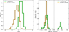 |
Fig. 5 Probability distributions of ftides (left) and λ3 (right) in protoclump regions (green histograms) and random patches (orange histograms). In the left panel, vertical lines of different colors indicate the median of the corresponding distribution, 0.33 and −0.27 for protoclumps and random patches, respectively. The ftides in protoclump regions are mostly positive, indicating substantial or fully compressive tides, while random patches mostly have ftides < 0, indicating substantial stripping. In the right panel, λ3 was scaled by 20 in order to separate negative and positive values and present them in a logarithmic scale. Negative values are actually − log(−20 · λ3) (e.g., a value of −5 along the x-axis represents −105 Gyr−1). We note that λ3 is positive almost exclusively in protoclump regions, and about ~25% of the protoclump regions have λ3 > 0, implying fully compressive tides. |
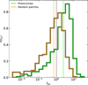 |
Fig. 6 Same as Figure 4 but for fstr, which measures the amount of stream mass in a given region (see text). The vertical black line is at fstr = 1. One can see that protoclump regions tend to have larger fstr than random patches, indicating that they reside in regions with intense accretion. The median fstr for protoclumps is 2.5, while for random patches it is 0.8. |
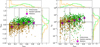 |
Fig. 7 Correlations between fconv (x-axis) and ftides (left) or fstr (right). Each point is either a protoclump (green points) or a random patch (orange points). The histograms are the projected distributions of the corresponding quantity. The vertical black lines correspond to fconv = 16% and fconv = 33%. The magenta squares are the medians of all of the points in bins of fconv, and the error bars are the 16th and 84th percentiles of each quantity. Both ftides and fstr show a positive correlation with fconv. The Spearman correlation coefficient for ftides and fstr against fconv are 0.46 and 0.3, with p-values of 2 · 10−3, 5 · 10−3, respectively. Furthermore, protoclump regions occupy the upper-right quadrants in both panels. |
4.2 Efficiency of stream-driven turbulence
When streams interact with a galactic disk, we expect them to drive turbulence within the disk. However, the efficiency of this stream-driven turbulence remains a topic of debate. Some studies suggest that accretion has little to no effect on disk turbulence (Hopkins et al. 2013), while others argue that its impact is weak (Elmegreen & Burkert 2010), occasionally significant (Gabor & Bournaud 2014), or even highly efficient (Forbes et al. 2023; Jiménez et al. 2023). If accretion-driven turbulence is indeed efficient, it could play a major role in sustaining overall disk turbulence (Ginzburg et al. 2022), particularly compressive turbulence. Preliminary controlled experiments investigating streams feeding a galactic disk (Ginzburg et al., in prep.) indicate that disks fed by streams tend to sustain larger values of velocity dispersions, with a strong dependence on the density of the incoming streams.
Stream density is expected to play a key role (Klessen & Hennebelle 2010), as basic momentum conservation suggests that more kinetic energy is retained in the system when the densities of the colliding materials are comparable14. Since the disk is built by the incoming material, streams cannot be much less dense than the outer disk. Moreover, simulations of streams feeding massive halos show that streams grow denser as they approach the inner halo (Aung et al. 2024), undergoing gravitational fragmentation along the way (Mandelker et al. 2018; Aung et al. 2019). Furthermore, Folini et al. (2014) found in simulations of head on collision of isothermal flows that high Mach number collisions are efficient at converting collision kinetic energy to turbulent kinetic energy, and produce a broader density distribution in the collision region.
Future work is planned to explore stream-disk interactions and the efficiency of accretion-driven turbulence, from cloud to galactic scales. These studies will also shed light on how compressive turbulence is driven in sites of stream-disk interaction.
4.3 Definition of compressive modes of turbulence
The motivation for the definition of fconv as defined in Eq. (9), is based on the Taylor expansion performed in Eq. (5) (see also Appendix B). This definitions neglects the shearing term, which we termed ![Mathematical equation: $\[\overleftrightarrow{S}\]$](/articles/aa/full_html/2025/06/aa53729-25/aa53729-25-eq23.png) , which is perhaps justified only for periodic or vanishing boundary conditions (Kritsuk et al. 2007), both of which are clearly irrelevant for our local analysis. We can gain qualitative insights on the relevance of
, which is perhaps justified only for periodic or vanishing boundary conditions (Kritsuk et al. 2007), both of which are clearly irrelevant for our local analysis. We can gain qualitative insights on the relevance of ![Mathematical equation: $\[\overleftrightarrow{S}\]$](/articles/aa/full_html/2025/06/aa53729-25/aa53729-25-eq24.png) from the following argument.
from the following argument.
The matrix ![Mathematical equation: $\[\overleftrightarrow{S}\]$](/articles/aa/full_html/2025/06/aa53729-25/aa53729-25-eq25.png) is a symmetric matrix, and hence it can be orthogonally diagonlized by three real eigenvalues, μ1 ≥ μ2 ≥ μ3. Furthermore, it is traceless, meaning that μ1 + μ2 + μ3 = 0. It therefore follows that μ1 ≥ 0 ≥ μ3, with μ2 somewhere in between. It means that the contribution from
is a symmetric matrix, and hence it can be orthogonally diagonlized by three real eigenvalues, μ1 ≥ μ2 ≥ μ3. Furthermore, it is traceless, meaning that μ1 + μ2 + μ3 = 0. It therefore follows that μ1 ≥ 0 ≥ μ3, with μ2 somewhere in between. It means that the contribution from ![Mathematical equation: $\[\overleftrightarrow{S}\]$](/articles/aa/full_html/2025/06/aa53729-25/aa53729-25-eq26.png) along the direction corresponding to μ3 is converging, while the contribution from
along the direction corresponding to μ3 is converging, while the contribution from ![Mathematical equation: $\[\overleftrightarrow{S}\]$](/articles/aa/full_html/2025/06/aa53729-25/aa53729-25-eq27.png) along the direction corresponding to μ1 is diverging. Since the sum of the eigenvalues is zero, μ1 and |μ3| can only differ at most by a factor of two. Thus, assuming μ1 ~ |μ3| is a reasonable approximation. We can then write the Taylor expansion of Eq. (5) in the coordinate system determined by
along the direction corresponding to μ1 is diverging. Since the sum of the eigenvalues is zero, μ1 and |μ3| can only differ at most by a factor of two. Thus, assuming μ1 ~ |μ3| is a reasonable approximation. We can then write the Taylor expansion of Eq. (5) in the coordinate system determined by ![Mathematical equation: $\[\overleftrightarrow{S}\]$](/articles/aa/full_html/2025/06/aa53729-25/aa53729-25-eq28.png) as
as
![Mathematical equation: $\[\boldsymbol{v}\left(\boldsymbol{r}+\delta \boldsymbol{r}^{\prime}\right) \approx \boldsymbol{v}+\left(\begin{array}{c}\left(1 / 3(\boldsymbol{\nabla} \cdot \boldsymbol{v})+\mu_1\right) \delta x^{\prime} \\1 / 3(\boldsymbol{\nabla} \cdot \boldsymbol{v}) \delta y^{\prime} \\\left(1 / 3(\boldsymbol{\nabla} \cdot \boldsymbol{v})-\mu_1\right) \delta z^{\prime}\end{array}\right)+\frac{1}{2} \omega^{\prime} \times \delta \boldsymbol{r}^{\prime},\]$](/articles/aa/full_html/2025/06/aa53729-25/aa53729-25-eq29.png) (16)
(16)
where primed values are the vectors in the lab frame represented in the coordinate frame of ![Mathematical equation: $\[\overleftrightarrow{S}\]$](/articles/aa/full_html/2025/06/aa53729-25/aa53729-25-eq30.png) . It is therefore evident that neglecting
. It is therefore evident that neglecting ![Mathematical equation: $\[\overleftrightarrow{S}\]$](/articles/aa/full_html/2025/06/aa53729-25/aa53729-25-eq31.png) is reasonable only if |∇ · v| ≫ μ1. However, for a region to become dense enough for self gravity to become efficient, isotropic collapse is not needed. It is therefore enough that ∇ · v < 0 and |∇ · v| ≳ μ1 so that the flow along the x′ will be weakly diverging, and the converging flow will occur along y′ and z′ direction.
is reasonable only if |∇ · v| ≫ μ1. However, for a region to become dense enough for self gravity to become efficient, isotropic collapse is not needed. It is therefore enough that ∇ · v < 0 and |∇ · v| ≳ μ1 so that the flow along the x′ will be weakly diverging, and the converging flow will occur along y′ and z′ direction.
When examining the simulations, we find that indeed usually μ2 ~ 0, while μ1 ~ |μ3|. protoclump regions usually have smaller shear eigenvalues than other random patches in the disk. Furthermore, we find that |∇ · v| ~ 2μ1 in protoclumps, while |∇ · v| ≲ μ1 in random patches. Alongside the sub-dominance of converging modes in random patches, we conclude that shear has a weaker effect in protoclump regions compared to random patches, which are more susceptible to shear, which prevents clump formation even when stellar feedback is weak (Fensch & Bournaud 2020). The increased shear can be due to the mean galactic rotation or the induction of strong shear in spiral arms. The exact cause of this shear should be explored in detailed, and is beyond the scope of this paper.
A more robust, multi scale method is required to go beyond the Helmholtz decomposition and Taylor approximation. A natural candidate is by utilizing wavelet transforms, which are common in turbulence studies in fluid dynamics (Farge 1992), but seem to be less common in galactic fluid dynamics. Not only that, but a locally orthogonal Helmholtz-like decomposition algorithm using wavelets has been formalized (Deriaz & Perrier 2009). Future work will be dedicated to performing turbulence decomposition using wavelets, with the potential for a more self-consistent quantification of compressive and solenoidal modes of turbulence.
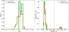 |
Fig. 8 Same as Figure 5 but for the protoclumps in the isolated galaxy simulation. One can see that the protoclumps in the isolated galaxy simulation are in regions where the tidal field is only weakly compressive, and are not much different than the random patches. Furthermore, λ3 < 0 for all of the protoclump regions, as opposed to protoclump regions in the cosmological simulations. |
5 Conclusions
By analyzing cosmological simulations of violent disks at 1 ≲z≲ 4, we studied the turbulent nature of protoclumps – regions out of which giant star-forming clumps form. Protoclump regions in the VELA cosmological simulations show local values of the Toomre-Q parameter greater than unity (sometimes substantially greater (Inoue et al. 2016)), indicating that their subsequent gravitational collapse is not initiated by linear gravitational instabilities. An excess in compressive modes of turbulence, and in particular converging modes, on the one hand increases the value of the velocity dispersion and therefore increases Q, but on the other hand, this excess causes the local material to become dense enough for self-gravity to eventually govern the collapse (Hopkins & Christiansen 2013).
By extending the sample size of galaxies and protoclump regions, we have strengthened the conclusion of M25, finding that protoclumps are dominated by converging modes of turbulence. In our extended sample, we find that approximately 50–70% of the turbulent kinetic energy in protoclumps is in converging modes, compared to ~16% expected in a fully isotropic and homogeneous turbulence in equipartition. Such an excess was not found in isolated galaxies, as we have shown in M25, implying that the cosmological environment or its influence on the galaxy causes its turbulence to be overly compressive.
We examined two external mechanisms for generating the excess of compressive turbulence, namely, compressive tides and interactions between the disk and dense streams accreting from the cosmic web. The messy environment of galaxies in a cosmological setting, including merging galaxies, gives rise to gravitational tides that can be substantially compressive and at times fully compressive (Dekel et al. 2003; Renaud et al. 2009; Li et al. 2022). We quantified the compressiveness of the tidal field by the dimensionless quantity ftides (Eq. (14)). We find that almost all protoclump regions have ftides > 0, indicating that they reside in regions where the tidal field is substantially compressive, with ftides ~0.32 on average. On the other hand, random patches in the disk have ftides ≲ 0, indicating that the tidal field in these regions is substantially expansive, at least along one direction. Furthermore, we found that ~25% of the protoclumps reside in regions where the tidal field is fully compressive, while practically no random patches are in regions of fully compressive tides.
High redshift massive galaxies in cosmological environments are fed by gaseous streams (typically three; Danovich et al. 2012; Codis et al. 2018). Upon impact, the streams can cause a strong compression due to shocks. We find that around 70% of the protoclump regions are sites of stream-disk interaction, containing approximately two to ten times as much stream material as the average at their galactocentric distance. Random patches, on the other hand, are more typical, with the mass of the stream material in their vicinity close to the average at their galactocentric distance. We therefore conclude that protoclump regions are distinct, both in terms of experiencing substantially compressive tides and residing in sites of stream-disk interaction.
We then examined how these two mechanisms correlate with the fraction of energy in compressive motion in the protoclumps and random patches in the disk. We found a positive correlation between the fraction of energy that is in compressive motion and the compressiveness of the tidal field in the region. Regions of the disk in which the tidal field is expansive typically have fconv ~ 0.16, which is the value expected for a fully isotropic and homogeneous turbulence in equipartition. As the tidal field becomes more compressive, the fraction of energy in converging modes increases to fconv ~ 0.6–0.7, on average. Similarly, we found a positive correlation between the intensity of the accreting streams in a given region to the fraction of energy in converging modes in the same region. Regions that are not intensely fed by streams have fconv ~ 0.16, while sites of stream-disk interaction have fconv ~ 0.5–0.7.
Our results suggest that both compressive tides and stream-disk interactions can drive compressive modes of turbulence. A more detailed investigation into the sources of compressive tides is required (see Sect. 4.1). However, an initial comparison with an isolated simulation suggests that these tides are not caused by the potential of the dark matter halo or the smooth disk component but instead arise either from external perturbations or from internal perturbations absent during clump formation in the isolated simulations. Furthermore, the lack of tracer particles in the VELA simulations makes the stream identification crude and noisy. We plan to perform a detailed analysis using cosmological simulations with tracer particles in order to properly isolate accreted material from the overall gas in the disk.
The results of Inoue et al. (2016), M25, and this study suggest that there is a need for a complementary physical theory of clump formation in cosmological disk galaxies. It is evident from these works that Toomre instability does not fully describe disk fragmentation in cosmological contexts. Furthermore, the results of Dutta Chowdhury et al. (2024) indicate that Toomre-based models for radial mass transport (Dekel et al. 2009; Krumholz & Burkert 2010) generally overpredict the radial velocities observed in numerical simulations. While Hopkins & Christiansen (2013) provide a turbulence-dependent stability threshold for Q based on a statistical analysis, a more thorough analysis based on first principles is required. Such a theory must take into account the balance between converging modes and solenoidal and diverging modes of turbulence. The former induces a local collapse, assisting gravity, while the latter prevent collapse, assisting rotation and shear.
Acknowledgements
This work was partly supported by ISF grant 861/20, BSF-NSF grant 2023723, and by BSF-NSF grant 2023730 and by grant JWST-AR-03305.005-A. N.M. acknowledges support from Israel Science Foundation (ISF) grant 3061/21. D.C. is a Ramon-Cajal Researcher and is supported by the Ministerio de Ciencia, Innovacion y Universidades (MICIU/FEDER) under research grant PID2021122603NB-C21. The VELA simulations were performed at the National Energy Research Scientific Computing Center (NERSC) at Lawrence Berkeley National Laboratory, and at NASA Advanced Supercomputing (NAS) at NASA Ames Research Center.
Appendix A Correspondence between the local and global decompositions
In this appendix we show that, if the compressive and solenoidal components have proportional power spectra, the correspondence indicated in eq. 10 holds. We start by writing the divergence and curl using the Fourier transform:
![Mathematical equation: $\[\nabla \times \boldsymbol{v}=\frac{1}{(2 \pi)^{3 / 2}} \int i \boldsymbol{k} \times \widetilde{\boldsymbol{v}}(\boldsymbol{k}) e^{i \boldsymbol{k} \cdot \boldsymbol{r}} d^3 \boldsymbol{k},\]$](/articles/aa/full_html/2025/06/aa53729-25/aa53729-25-eq32.png) (A.1)
(A.1)
![Mathematical equation: $\[\nabla \cdot \boldsymbol{v}=\frac{1}{(2 \pi)^{3 / 2}} \int i \boldsymbol{k} \cdot \widetilde{\boldsymbol{v}}(\boldsymbol{k}) e^{i \boldsymbol{k} \cdot \boldsymbol{r}} d^3 \boldsymbol{k},\]$](/articles/aa/full_html/2025/06/aa53729-25/aa53729-25-eq33.png) (A.2)
(A.2)
where ![Mathematical equation: $\[\widetilde{\boldsymbol{v}}\]$](/articles/aa/full_html/2025/06/aa53729-25/aa53729-25-eq34.png) is the Fourier transform of v. Using Parseval’s identity, we can write
is the Fourier transform of v. Using Parseval’s identity, we can write
![Mathematical equation: $\[\int|\nabla \times \boldsymbol{v}|^2 d^3 \boldsymbol{r}=\int|\boldsymbol{k} \times \widetilde{\boldsymbol{v}}|^2 d^3 \boldsymbol{k},\]$](/articles/aa/full_html/2025/06/aa53729-25/aa53729-25-eq35.png) (A.3)
(A.3)
![Mathematical equation: $\[\int|\nabla \cdot \boldsymbol{v}|^2 d^3 \boldsymbol{r}=\int|\boldsymbol{k} \cdot \widetilde{\boldsymbol{v}}|^2 d^3 \boldsymbol{k}.\]$](/articles/aa/full_html/2025/06/aa53729-25/aa53729-25-eq36.png) (A.4)
(A.4)
Next, we can write ![Mathematical equation: $\[\widetilde{v}=\widetilde{\boldsymbol{v}}_{\text {comp }}+\widetilde{\boldsymbol{v}}_{\text {sol }}\]$](/articles/aa/full_html/2025/06/aa53729-25/aa53729-25-eq37.png) (see eq. 2). We note that
(see eq. 2). We note that ![Mathematical equation: $\[\widetilde{\boldsymbol{v}}_{\text {comp }} \| \boldsymbol{k}\]$](/articles/aa/full_html/2025/06/aa53729-25/aa53729-25-eq38.png) , while
, while ![Mathematical equation: $\[\widetilde{\boldsymbol{v}}_{\text {sol }} \perp \boldsymbol{k}\]$](/articles/aa/full_html/2025/06/aa53729-25/aa53729-25-eq39.png) . We can therefore rewrite eqs. A.3 and A.4 as
. We can therefore rewrite eqs. A.3 and A.4 as
![Mathematical equation: $\[\int|\nabla \times \boldsymbol{v}|^2 d^3 \boldsymbol{r}=\int|\boldsymbol{k}|^2\left|\overline{\boldsymbol{v}}_{\mathrm{sol}}\right|^2 d^3 \boldsymbol{k},\]$](/articles/aa/full_html/2025/06/aa53729-25/aa53729-25-eq40.png) (A.5)
(A.5)
![Mathematical equation: $\[\int|\nabla \cdot \boldsymbol{v}|^2 d^3 \boldsymbol{r}=\int|\boldsymbol{k}|^2\left|\widetilde{\boldsymbol{v}}_{\text {comp }}\right|^2 d^3 \boldsymbol{k}.\]$](/articles/aa/full_html/2025/06/aa53729-25/aa53729-25-eq41.png) (A.6)
(A.6)
So far, we have not made any assumption about the statistical nature of the velocity field. Next, we assume that ![Mathematical equation: $\[\left|\widetilde{\boldsymbol{v}}_{\text {sol }}\right|^{2}=\alpha\left|\widetilde{\boldsymbol{v}}_{\text {comp }}\right|^{2}\]$](/articles/aa/full_html/2025/06/aa53729-25/aa53729-25-eq42.png) , where α is a constant in a homogeneous turbulence. This assumption implies that the driving scale and turbulence cascade of both the compressive and solenoidal components are the same. We can therefore write
, where α is a constant in a homogeneous turbulence. This assumption implies that the driving scale and turbulence cascade of both the compressive and solenoidal components are the same. We can therefore write
![Mathematical equation: $\[\begin{aligned}& \frac{\int|\nabla \cdot \boldsymbol{v}|^2 d^3 \boldsymbol{r}}{\int|\nabla \cdot \boldsymbol{v}|^2 d^3 \boldsymbol{r}+\int|\nabla \times \boldsymbol{v}|^2 d^3 \boldsymbol{r}}= \\& \frac{\int|\boldsymbol{k}|^2\left|\widetilde{\boldsymbol{v}}_{\text {comp }}\right|^2 d^3 \boldsymbol{k}}{\int|\boldsymbol{k}|^2\left|\widetilde{\boldsymbol{v}}_{\text {comp }}\right|^2 d^3 \boldsymbol{k}+\int|\boldsymbol{k}|^2\left|\widetilde{\boldsymbol{v}}_{\text {sol }}\right|^2 d^3 \boldsymbol{k}}= \\& \frac{\int|\boldsymbol{k}|^2\left|\widetilde{\boldsymbol{v}}_{\text {comp }}\right|^2 d^3 \boldsymbol{k}}{\int|\boldsymbol{k}|^2\left|\widetilde{\boldsymbol{v}}_{\text {comp }}\right|^2 d^3 \boldsymbol{k}+\alpha \int|\boldsymbol{k}|^2\left|\widetilde{\boldsymbol{v}}_{\text {comp }}\right|^2 d^3 \boldsymbol{k}}=\frac{1}{1+\alpha}.\end{aligned}\]$](/articles/aa/full_html/2025/06/aa53729-25/aa53729-25-eq43.png) (A.7)
(A.7)
Furthermore, again exploiting Parseval’s theorem,
![Mathematical equation: $\[\begin{aligned}& \frac{\int\left|\boldsymbol{v}_{\text {comp }}\right|^2 d^3 \boldsymbol{r}}{\int|\boldsymbol{v}|^2 d^3 \boldsymbol{r}}= \\& \frac{\int\left|\boldsymbol{v}_{\text {comp }}\right|^2 d^3 \boldsymbol{r}}{\int\left|\boldsymbol{v}_{\text {comp }}\right|^2 d^3 \boldsymbol{r}+\int\left|\boldsymbol{v}_{\text {sol }}\right|^2 d^3 \boldsymbol{r}}= \\& \frac{\int\left|\widetilde{\boldsymbol{v}}_{\text {comp }}\right|^2 d^3 \boldsymbol{k}}{\int\left|\widetilde{\boldsymbol{v}}_{\text {comp }}\right|^2 d^3 \boldsymbol{k}+\int\left|\widetilde{\boldsymbol{v}}_{\text {sol }}\right|^2 d^3 \boldsymbol{k}}= \\& \frac{\int\left|\widetilde{\boldsymbol{v}}_{\text {comp }}\right|^2 d^3 \boldsymbol{k}}{\int\left|\widetilde{\boldsymbol{v}}_{\text {comp }}\right|^2 d^3 \boldsymbol{k}+\alpha \int\left|\widetilde{\boldsymbol{v}}_{\text {comp }}\right|^2 d^3 \boldsymbol{k}}=\frac{1}{1+\alpha}.\end{aligned}\]$](/articles/aa/full_html/2025/06/aa53729-25/aa53729-25-eq44.png) (A.8)
(A.8)
We can therefore see that the equality of eq. 10 holds.
Appendix B Viscous dissipation decomposition
The viscous dissipation rate per unit volume of a compressible fluid is given by (Chandrasekhar 1961)
![Mathematical equation: $\[\Phi=2 \mu\left(e_{i j} e_{i j}-\frac{1}{3}\left(e_{i i}\right)^2\right),\]$](/articles/aa/full_html/2025/06/aa53729-25/aa53729-25-eq45.png) (B.1)
(B.1)
where μ is the dynamic viscosity, eij = 1/2(∂vi/∂rj + ∂vj/∂ri), and we have employed the summation notation. We note that since repeated indices are summed over,
![Mathematical equation: $\[e_{i j} e_{i j}=\frac{1}{4}\left(\frac{\partial v_i}{\partial r_j} \frac{\partial v_i}{\partial r_j}+\frac{\partial v_j}{\partial r_i} \frac{\partial v_j}{\partial r_i}+2 \frac{\partial v_i}{\partial r_j} \frac{\partial v_j}{\partial r_i}\right)=\frac{1}{2}\left(\frac{\partial v_i}{\partial r_j} \frac{\partial v_i}{\partial r_j}+\frac{\partial v_i}{\partial r_j} \frac{\partial v_j}{\partial r_i}\right).\]$](/articles/aa/full_html/2025/06/aa53729-25/aa53729-25-eq46.png) (B.2)
(B.2)
Furthermore,
![Mathematical equation: $\[\begin{aligned}|\nabla \times \boldsymbol{v}|^2 & =\epsilon_{k i j} \frac{\partial v_j}{\partial r_i} \epsilon_{k l m} \frac{\partial v_m}{\partial r_l}=\left(\delta_{i l} \delta_{j m}-\delta_{i m} \delta_{j l}\right) \frac{\partial v_i}{\partial r_j} \frac{\partial v_l}{\partial r_m} \\& =\frac{\partial v_i}{\partial r_j} \frac{\partial v_i}{\partial r_j}-\frac{\partial v_i}{\partial r_j} \frac{\partial v_j}{\partial r_i}.\end{aligned}\]$](/articles/aa/full_html/2025/06/aa53729-25/aa53729-25-eq47.png) (B.3)
(B.3)
Here, εkij is the Levi-Civita symbol and δij is the Kronecker delta. Plugging into eq. B.2, we get
![Mathematical equation: $\[e_{i j} e_{i j}=\frac{1}{2}\left(|\nabla \times \boldsymbol{v}|^2+2 \frac{\partial v_i}{\partial r_j} \frac{\partial v_j}{\partial r_i}\right).\]$](/articles/aa/full_html/2025/06/aa53729-25/aa53729-25-eq48.png) (B.4)
(B.4)
Next, we write
![Mathematical equation: $\[\frac{\partial v_i}{\partial r_j} \frac{\partial v_j}{\partial r_i}=\frac{\partial v_i}{\partial r_j} \frac{\partial v_j}{\partial r_i}-\frac{\partial v_i}{\partial r_i} \frac{\partial v_j}{\partial r_j}+\frac{\partial v_i}{\partial r_i} \frac{\partial v_j}{\partial r_j}=\frac{\partial v_i}{\partial r_j} \frac{\partial v_j}{\partial r_i}-\frac{\partial v_i}{\partial r_i} \frac{\partial v_j}{\partial r_j}+\left(e_{i i}\right)^2.\]$](/articles/aa/full_html/2025/06/aa53729-25/aa53729-25-eq49.png) (B.5)
(B.5)
Using the product rule,
![Mathematical equation: $\[\begin{aligned}& \frac{\partial v_i}{\partial r_j} \frac{\partial v_j}{\partial r_i}=\frac{\partial}{\partial r_j}\left(v_i \frac{\partial v_j}{\partial r_i}\right)-v_i \frac{\partial^2 v_j}{\partial r_j \partial r_i}, \\& \frac{\partial v_i}{\partial r_i} \frac{\partial v_j}{\partial r_j}=\frac{\partial}{\partial r_j}\left(v_j \frac{\partial v_i}{\partial r_i}\right)-v_j \frac{\partial^2 v_i}{\partial r_i \partial r_j}.\end{aligned}\]$](/articles/aa/full_html/2025/06/aa53729-25/aa53729-25-eq50.png)
Subtracting, as in eq. B.5, and by changing i ↔ j in the second term on the right hand side of the second line, we get
![Mathematical equation: $\[\frac{\partial v_i}{\partial r_j} \frac{\partial v_j}{\partial r_i}-\frac{\partial v_i}{\partial r_i} \frac{\partial v_j}{\partial r_j}=\frac{\partial}{\partial r_j}\left(v_i \frac{\partial v_j}{\partial r_i}-v_j \frac{\partial v_i}{\partial r_i}\right).\]$](/articles/aa/full_html/2025/06/aa53729-25/aa53729-25-eq51.png) (B.6)
(B.6)
Plugging this into B.5, and then to B.4, we get
![Mathematical equation: $\[e_{i j} e_{i j}=\frac{1}{2}\left(|\nabla \times \boldsymbol{v}|^2+\boldsymbol{\nabla} \cdot(\overleftrightarrow{D} \boldsymbol{v})+2\left(e_{i i}\right)^2\right),\]$](/articles/aa/full_html/2025/06/aa53729-25/aa53729-25-eq52.png) (B.7)
(B.7)
where we have defined Dij = 2 ∂vj/∂ri − 2(∇ · v) δij. Wrapping everything back to eq. B.1, we get
![Mathematical equation: $\[\Phi=\mu|\nabla \times \boldsymbol{v}|^2+\frac{4}{3} \mu(\nabla \cdot \boldsymbol{v})^2+\mu \boldsymbol{\nabla} \cdot(\overleftrightarrow{D} \boldsymbol{v}.)\]$](/articles/aa/full_html/2025/06/aa53729-25/aa53729-25-eq53.png) (B.8)
(B.8)
Thus, the total viscous dissipation rate in a given volume, V, is
![Mathematical equation: $\[\epsilon=\int \Phi d^3 \boldsymbol{r}=\mu \int_V\left(|\nabla \times \boldsymbol{v}|^2+\frac{4}{3}(\nabla \cdot \boldsymbol{v})^2\right) d^3 \boldsymbol{r}+\mu \int_{\partial V}(\overleftrightarrow{D} \boldsymbol{v}) \cdot d^2 \boldsymbol{r},\]$](/articles/aa/full_html/2025/06/aa53729-25/aa53729-25-eq54.png) (B.9)
(B.9)
where we have used the divergence theorem to turn the volume integral of ![Mathematical equation: $\[\nabla \cdot(\overleftrightarrow{D} \boldsymbol{v})\]$](/articles/aa/full_html/2025/06/aa53729-25/aa53729-25-eq55.png) into a surface integral. From eq. B.9, we learned that the viscous dissipation rate, and hence the turbulence dissipation rate, is affected not only by the curl and the divergence of the velocity field inside the volume (Kida & Orszag 1990) but also by a surface term. This surface term vanishes only for specific boundary conditions, such as periodic and vanishing at infinity. In these cases, if one thinks of the viscous dissipation rate as the energy injection rate to turbulence, one can qualitatively expect that the total energy in compressive modes of turbulence is ∝ |∇ · v|2, and the total energy in solenoidal modes is ∝|∇ × v|2.
into a surface integral. From eq. B.9, we learned that the viscous dissipation rate, and hence the turbulence dissipation rate, is affected not only by the curl and the divergence of the velocity field inside the volume (Kida & Orszag 1990) but also by a surface term. This surface term vanishes only for specific boundary conditions, such as periodic and vanishing at infinity. In these cases, if one thinks of the viscous dissipation rate as the energy injection rate to turbulence, one can qualitatively expect that the total energy in compressive modes of turbulence is ∝ |∇ · v|2, and the total energy in solenoidal modes is ∝|∇ × v|2.
References
- Agertz, O., Lake, G., Teyssier, R., et al. 2009a, MNRAS, 392, 294 [NASA ADS] [CrossRef] [Google Scholar]
- Agertz, O., Teyssier, R., & Moore, B. 2009b, MNRAS, 397, L64 [NASA ADS] [CrossRef] [Google Scholar]
- Aluie, H. 2013, Phys. D Nonlinear Phenom., 247, 54 [Google Scholar]
- Arora, R., Federrath, C., Krumholz, M., & Banerjee, R. 2025, A&A, 695, A155 [NASA ADS] [CrossRef] [EDP Sciences] [Google Scholar]
- Aung, H., Mandelker, N., Nagai, D., Dekel, A., & Birnboim, Y. 2019, MNRAS, 490, 181 [NASA ADS] [CrossRef] [Google Scholar]
- Aung, H., Mandelker, N., Dekel, A., et al. 2024, MNRAS, 532, 2965 [NASA ADS] [CrossRef] [Google Scholar]
- Binney, J., & Tremaine, S. 2008, Galactic Dynamics, 2nd edn. (Berlin: Springer) [Google Scholar]
- Bournaud, F., & Elmegreen, B. G. 2009, ApJ, 694, L158 [CrossRef] [Google Scholar]
- Bournaud, F., Elmegreen, B. G., Teyssier, R., Block, D. L., & Puerari, I. 2010, MNRAS, 409, 1088 [CrossRef] [Google Scholar]
- Bournaud, F., Perret, V., Renaud, F., et al. 2014, ApJ, 780, 57 [Google Scholar]
- Brunt, C. M., & Federrath, C. 2014, MNRAS, 442, 1451 [Google Scholar]
- Cava, A., Schaerer, D., Richard, J., et al. 2018, Nat. Astron., 2, 76 [Google Scholar]
- Ceverino, D., & Klypin, A. 2009, ApJ, 695, 292 [Google Scholar]
- Ceverino, D., Dekel, A., & Bournaud, F. 2010, MNRAS, 404, 2151 [NASA ADS] [Google Scholar]
- Ceverino, D., Dekel, A., Mandelker, N., et al. 2012, MNRAS, 420, 3490 [NASA ADS] [CrossRef] [Google Scholar]
- Ceverino, D., Klypin, A., Klimek, E. S., et al. 2014, MNRAS, 442, 1545 [NASA ADS] [CrossRef] [Google Scholar]
- Ceverino, D., Mandelker, N., Snyder, G. F., et al. 2023, MNRAS, 522, 3912 [NASA ADS] [CrossRef] [Google Scholar]
- Chandrasekhar, S. 1961, Hydrodynamic and Hydromagnetic Stability (North Chelmsford, Massachusett: Courier Corporation) [Google Scholar]
- Codis, S., Pogosyan, D., & Pichon, C. 2018, MNRAS, 479, 973 [Google Scholar]
- Danovich, M., Dekel, A., Hahn, O., & Teyssier, R. 2012, MNRAS, 422, 1732 [Google Scholar]
- Dekel, A., & Burkert, A. 2014, MNRAS, 438, 1870 [Google Scholar]
- Dekel, A., Devor, J., & Hetzroni, G. 2003, MNRAS, 341, 326 [Google Scholar]
- Dekel, A., Sari, R., & Ceverino, D. 2009, ApJ, 703, 785 [Google Scholar]
- Dekel, A., Ginzburg, O., Jiang, F., et al. 2020, MNRAS, 493, 4126 [CrossRef] [Google Scholar]
- Dekel, A., Mandelker, N., Bournaud, F., et al. 2022, MNRAS, 511, 316 [NASA ADS] [CrossRef] [Google Scholar]
- Dekel, A., Tziperman, O., Sarkar, K. C., et al. 2023, MNRAS, 521, 4299 [NASA ADS] [CrossRef] [Google Scholar]
- Deriaz, E., & Perrier, V. 2009, Appl. Comput. Harmonic Anal., 26, 249 [Google Scholar]
- Dutta Chowdhury, D., Dekel, A., Mandelker, N., Ginzburg, O., & Genzel, R. 2024, A&A, submitted [arXiv:2409.01589] [Google Scholar]
- Ejdetjärn, T., Agertz, O., Östlin, G., Renaud, F., & Romeo, A. B. 2022, MNRAS, 514, 480 [CrossRef] [Google Scholar]
- Elmegreen, B. G. 2011, ApJ, 737, 10 [NASA ADS] [CrossRef] [Google Scholar]
- Elmegreen, B. G., & Burkert, A. 2010, ApJ, 712, 294 [Google Scholar]
- Farge, M. 1992, Ann. Rev. Fluid Mech., 24, 395 [Google Scholar]
- Federrath, C. 2018, Phys. Today, 71, 38 [NASA ADS] [CrossRef] [Google Scholar]
- Federrath, C., & Klessen, R. S. 2012, ApJ, 761, 156 [Google Scholar]
- Federrath, C., Roman-Duval, J., Klessen, R. S., Schmidt, W., & Mac Low, M. M. 2010, A&A, 512, A81 [NASA ADS] [CrossRef] [EDP Sciences] [Google Scholar]
- Federrath, C., Rathborne, J. M., Longmore, S. N., et al. 2017, IAU Symp., 322, 123 [Google Scholar]
- Federrath, C., Klessen, R. S., Iapichino, L., & Beattie, J. R. 2021, Nat. Astron., 5, 365 [NASA ADS] [CrossRef] [Google Scholar]
- Fensch, J., & Bournaud, F. 2020, arXiv e-prints [arXiv:2011.12966] [Google Scholar]
- Fensch, J., Bournaud, F., Brucy, N., et al. 2023, A&A, 672, A193 [NASA ADS] [CrossRef] [EDP Sciences] [Google Scholar]
- Fisher, D. B., Glazebrook, K., Abraham, R. G., et al. 2017, ApJ, 839, L5 [NASA ADS] [CrossRef] [Google Scholar]
- Folini, D., Walder, R., & Favre, J. M. 2014, A&A, 562, A112 [NASA ADS] [CrossRef] [EDP Sciences] [Google Scholar]
- Forbes, J. C., Emami, R., Somerville, R. S., et al. 2023, ApJ, 948, 107 [NASA ADS] [CrossRef] [Google Scholar]
- Förster Schreiber, N. M., Shapley, A. E., Genzel, R., et al. 2011, ApJ, 739, 45 [Google Scholar]
- Förster Schreiber, N. M., Übler, H., Davies, R. L., et al. 2019, ApJ, 875, 21 [Google Scholar]
- Fujimoto, S., Ouchi, M., Kohno, K., et al. 2024, arXiv e-prints [arXiv:2402.18543] [Google Scholar]
- Gabor, J. M., & Bournaud, F. 2014, MNRAS, 437, L56 [Google Scholar]
- Garnier, E., Adams, N., & Sagaut, P. 2009, Large Eddy Simulation for Compressible Flows (Berlin: Springer) [CrossRef] [Google Scholar]
- Genzel, R., Burkert, A., Bouché, N., et al. 2008, ApJ, 687, 59 [Google Scholar]
- Genzel, R., Newman, S., Jones, T., et al. 2011, ApJ, 733, 101 [Google Scholar]
- Genzel, R., Förster Schreiber, N. M., Lang, P., et al. 2014, ApJ, 785, 75 [NASA ADS] [CrossRef] [Google Scholar]
- Genzel, R., Jolly, J. B., Liu, D., et al. 2023, ApJ, 957, 48 [NASA ADS] [CrossRef] [Google Scholar]
- Ginzburg, O., Huertas-Company, M., Dekel, A., et al. 2021, MNRAS, 501, 730 [Google Scholar]
- Ginzburg, O., Dekel, A., Mandelker, N., & Krumholz, M. R. 2022, MNRAS, 513, 6177 [NASA ADS] [CrossRef] [Google Scholar]
- Goldbaum, N. J., Krumholz, M. R., & Forbes, J. C. 2015, ApJ, 814, 131 [NASA ADS] [CrossRef] [Google Scholar]
- Goldreich, P., & Lynden-Bell, D. 1965, MNRAS, 130, 97 [NASA ADS] [CrossRef] [Google Scholar]
- Griv, E., & Gedalin, M. 2012, MNRAS, 422, 600 [NASA ADS] [CrossRef] [Google Scholar]
- Guo, Y., Ferguson, H. C., Bell, E. F., et al. 2015, ApJ, 800, 39 [NASA ADS] [CrossRef] [Google Scholar]
- Guo, Y., Rafelski, M., Bell, E. F., et al. 2018, ApJ, 853, 108 [NASA ADS] [CrossRef] [Google Scholar]
- Hennebelle, P., & Falgarone, E. 2012, A&A Rev., 20, 55 [NASA ADS] [CrossRef] [Google Scholar]
- Hopkins, P. F., & Christiansen, J. L. 2013, ApJ, 776, 48 [Google Scholar]
- Hopkins, P. F., Quataert, E., & Murray, N. 2012, MNRAS, 421, 3488 [NASA ADS] [CrossRef] [Google Scholar]
- Hopkins, P. F., Kereš, D., & Murray, N. 2013, MNRAS, 432, 2639 [NASA ADS] [CrossRef] [Google Scholar]
- Huertas-Company, M., Guo, Y., Ginzburg, O., et al. 2020, MNRAS, 499, 814 [NASA ADS] [CrossRef] [Google Scholar]
- Immeli, A., Samland, M., Westera, P., & Gerhard, O. 2004, ApJ, 611, 20 [CrossRef] [Google Scholar]
- Inoue, S., & Yoshida, N. 2018, MNRAS, 474, 3466 [Google Scholar]
- Inoue, S., Dekel, A., Mandelker, N., et al. 2016, MNRAS, 456, 2052 [CrossRef] [Google Scholar]
- Jiménez, E., Lagos, C. d. P., Ludlow, A. D., & Wisnioski, E. 2023, MNRAS, 524, 4346 [CrossRef] [Google Scholar]
- Jog, C. J. 2014, AJ, 147, 132 [NASA ADS] [CrossRef] [Google Scholar]
- Kalita, B. S., Silverman, J. D., Daddi, E., et al. 2024, ApJ, 960, 25 [NASA ADS] [CrossRef] [Google Scholar]
- Kassin, S. A., Weiner, B. J., Faber, S. M., et al. 2012, ApJ, 758, 106 [NASA ADS] [CrossRef] [Google Scholar]
- Kida, S., & Orszag, S. A. 1990, J. Sci. Comput., 5, 85 [NASA ADS] [CrossRef] [Google Scholar]
- Klessen, R. S., & Hennebelle, P. 2010, A&A, 520, A17 [NASA ADS] [CrossRef] [Google Scholar]
- Kravtsov, A. V., Klypin, A. A., & Khokhlov, A. M. 1997, ApJS, 111, 73 [Google Scholar]
- Kritsuk, A. G., Norman, M. L., Padoan, P., & Wagner, R. 2007, ApJ, 665, 416 [NASA ADS] [CrossRef] [Google Scholar]
- Kritsuk, A. G., Nordlund, Å., Collins, D., et al. 2011, ApJ, 737, 13 [NASA ADS] [CrossRef] [Google Scholar]
- Krumholz, M., & Burkert, A. 2010, ApJ, 724, 895 [NASA ADS] [CrossRef] [Google Scholar]
- Krumholz, M. R., Burkhart, B., Forbes, J. C., & Crocker, R. M. 2018, MNRAS, 477, 2716 [CrossRef] [Google Scholar]
- Lapiner, S., Dekel, A., Freundlich, J., et al. 2023, MNRAS, 522, 4515 [NASA ADS] [CrossRef] [Google Scholar]
- Li, H., Vogelsberger, M., Bryan, G. L., et al. 2022, MNRAS, 514, 265 [NASA ADS] [CrossRef] [Google Scholar]
- Livermore, R. C., Jones, T. A., Richard, J., et al. 2015, MNRAS, 450, 1812 [Google Scholar]
- Lovelace, R. V. E., & Hohlfeld, R. G. 1978, ApJ, 221, 51 [NASA ADS] [CrossRef] [Google Scholar]
- Mandelker, N., Dekel, A., Ceverino, D., et al. 2017, MNRAS, 464, 635 [NASA ADS] [CrossRef] [Google Scholar]
- Mandelker, N., van Dokkum, P. G., Brodie, J. P., van den Bosch, F. C., & Ceverino, D. 2018, ApJ, 861, 148 [NASA ADS] [CrossRef] [Google Scholar]
- Mandelker, N., Nagai, D., Aung, H., et al. 2020, MNRAS, 494, 2641 [Google Scholar]
- Mandelker, N., Ginzburg, O., Dekel, A., et al. 2025, MNRAS, 538, L9 [Google Scholar]
- Mayer, L., Tamburello, V., Lupi, A., et al. 2016, ApJ, 830, L13 [NASA ADS] [CrossRef] [Google Scholar]
- Meng, X., & Gnedin, O. Y. 2020, MNRAS, 494, 1263 [Google Scholar]
- Muratov, A. L., Kereš, D., Faucher-Giguère, C.-A., et al. 2015, MNRAS, 454, 2691 [NASA ADS] [CrossRef] [Google Scholar]
- Nakazato, Y., Ceverino, D., & Yoshida, N. 2024, arXiv e-prints [arXiv:2402.08911] [Google Scholar]
- Noguchi, M. 1999, ApJ, 514, 77 [NASA ADS] [CrossRef] [Google Scholar]
- Ogiya, G., & Nagai, D. 2022, MNRAS, 514, 555 [Google Scholar]
- Oklopčić, A., Hopkins, P. F., Feldmann, R., et al. 2017, MNRAS, 465, 952 [CrossRef] [Google Scholar]
- Padoan, P., & Nordlund, Å. 2002, ApJ, 576, 870 [NASA ADS] [CrossRef] [Google Scholar]
- Rafikov, R. R. 2001, MNRAS, 323, 445 [NASA ADS] [CrossRef] [Google Scholar]
- Renaud, F., Boily, C. M., Naab, T., & Theis, C. 2009, ApJ, 706, 67 [NASA ADS] [CrossRef] [Google Scholar]
- Renaud, F., Bournaud, F., Kraljic, K., & Duc, P. A. 2014, MNRAS, 442, L33 [NASA ADS] [CrossRef] [Google Scholar]
- Renaud, F., Romeo, A. B., & Agertz, O. 2021, MNRAS, 508, 352 [NASA ADS] [CrossRef] [Google Scholar]
- Renaud, F., Segovia Otero, Á., & Agertz, O. 2022, MNRAS, 516, 4922 [NASA ADS] [CrossRef] [Google Scholar]
- Renaud, F., Agertz, O., & Romeo, A. B. 2024, A&A, 687, A91 [NASA ADS] [CrossRef] [EDP Sciences] [Google Scholar]
- Romeo, A. B. 1994, A&A, 286, 799 [NASA ADS] [Google Scholar]
- Romeo, A. B., & Falstad, N. 2013, MNRAS, 433, 1389 [NASA ADS] [CrossRef] [Google Scholar]
- Romeo, A. B., & Wiegert, J. 2011, MNRAS, 416, 1191 [NASA ADS] [CrossRef] [Google Scholar]
- Rowland, L. E., Hodge, J., Bouwens, R., et al. 2024, arXiv e-prints [arXiv:2405.06025] [Google Scholar]
- Sattari, Z., Mobasher, B., Chartab, N., et al. 2023, ApJ, 951, 147 [NASA ADS] [CrossRef] [Google Scholar]
- Schmidt, W. 2014, Numerical Modelling of Astrophysical Turbulence (Berlin: Springer) [CrossRef] [Google Scholar]
- Schmidt, W., Niemeyer, J. C., & Hillebrandt, W. 2006, A&A, 450, 265 [NASA ADS] [CrossRef] [EDP Sciences] [Google Scholar]
- Semenov, V. A. 2024, arXiv e-prints [arXiv:2410.23339] [Google Scholar]
- Shibuya, T., Ouchi, M., Kubo, M., & Harikane, Y. 2016, ApJ, 821, 72 [NASA ADS] [CrossRef] [Google Scholar]
- Swinbank, A. M., Smail, I., Sobral, D., et al. 2012, ApJ, 760, 130 [NASA ADS] [CrossRef] [Google Scholar]
- Toomre, A. 1964, ApJ, 139, 1217 [Google Scholar]
- Wuyts, S., Förster Schreiber, N. M., Genzel, R., et al. 2012, ApJ, 753, 114 [NASA ADS] [CrossRef] [Google Scholar]
- Zanella, A., Le Floc’h, E., Harrison, C. M., et al. 2019, MNRAS, 489, 2792 [Google Scholar]
- Zanella, A., Iani, E., Dessauges-Zavadsky, M., et al. 2024, A&A, 685, A80 [NASA ADS] [CrossRef] [EDP Sciences] [Google Scholar]
- Zolotov, A., Dekel, A., Mandelker, N., et al. 2015, MNRAS, 450, 2327 [Google Scholar]
Hopkins & Christiansen (2013) found that for highly supersonic turbulence, a disk is never statistically stable. Their study focused on protoplanetary disks. However, adopting model parameters suited to galactic disks, where turbulence is driven by multiple mechanisms with significant morphological variations, suggests a more appropriate Q threshold is ~5.
The galaxies we analyze are labeled V07, V08, V11, V12, V14, V25, V26 and V27, in accordance with table 1 in Mandelker et al. (2017).
The galactic disk’s dimensions and orientation are defined by those of the cylinder that contains 85% of the cold component, consisting of gas with T < 104 K and young stars with age <100 Myr, within 0.15Rvir (Mandelker et al. 2017).
The former is the more general notion of allowing supersonic flows and shocks, while the latter generally refers to the tendency of the velocity field to converge to a point.
Suppose ∇ψ = 0 on the boundary. Let D0 be some arbitrarily chosen point on the boundary. Then, if D is any point on the boundary, ψ(D) − ψ(D0) = ∫ ∇ψ · dl = 0, where the integration is along the boundary. This shows that ψ(D) = ψ(D0) for all points D on the boundary. Thus, ψ solves the Laplace equation with ψ = const. on the boundary. From the uniqueness theorem for Laplace’s equation, ψ = const. in the entire volume.
We have that |v|2 = |vcomp|2 + |vsol|2 + 2vcomp · vsol, where the last term is, in general, not zero.
That is, a velocity field whose two-point correlation function is a function of the magnitude of the separation only.
If the rotation velocity, vϕ, is varies slowly on the scales of the protoclump, then ∇ · v = ∇ · (vϕ + Δv) ≈ ∇ · (Δv).
The divergence part is smaller than the curl part by a factor of 2/3. This amounts to a factor of ~0.8 in the local fraction as defined in Eq. (9), which doesn’t affect the qualitative results.
Other possible reasonings behind this definition are either the correspondence with the Helmholtz decomposition, Eq. (10), or from the fact that the viscous dissipation rate can be decomposed to a solenoidal and compressive part, as shown in Appendix B. Both of these explanations rely on specific boundary conditions.
We note that other publications (e.g., Renaud et al. 2009) defined the tidal tensor with a minus sign. Under such a definition, a positive (negative) eigenvalue represents disruption (compression) rather than compression (disruption).
Our calculation resulted in Ft = −(R/4)λ1(1 + ftides), which is positive only when ftides < −1, meaning that the mean acceleration is positive only when ftides < −1. Nevertheless, substantial tidal stripping can occur along a particular direction even if the mean acceleration is negative.
As can be seen in Figure 1 in Renaud et al. (2014), a galaxy in isolation attains equipartition within a couple of dynamical times.
For instance, in a simple, perfectly inelastic collision, the fraction of kinetic energy retained in the system is proportional to δ/(1 + δ), where δ is the density contrast between the colliding materials. While this relationship may differ in fluid collisions, it highlights the significance of density contrast in such interactions.
All Figures
|
Fig. 1 Proof of concept for fstr. The background color shows the projected surface density of gas in V07 at z ~ 2 (top) and in V08 at z ~ 1 (bottom). The contours are of fstr in angular bins at a radius of 8 kpc in both panels. One can see how fstr increases in regions where the stream interacts with the disk. |
| In the text | |
|
Fig. 2 Temporal evolution of the global fraction of turbulent energy in converging and diverging flows (blue curve) and in only converging (i.e., only cells with ∇ · v < 0; red curve) flows for three galaxies from our suite. The vertical black line indicates the moment of the blue nugget phase in each galaxy (Lapiner et al. 2023). The horizontal solid (dashed) lines indicate one third (sixth) of the total energy, values expected for fully isotropic and homogeneous turbulence in equipartition. Each of the blue nugget phases are preceded by at least one major merger, which increases the global fraction in compressive turbulence, before settling back to the equilibrium values. |
| In the text | |
|
Fig. 3 Correlation of fconv with gas density in protoclump regions. In the left panels, we show the projected surface density of the gas. The top row represents V07 at z ~ 2, while the bottom row represents V08 at z ~ 1, as in Figure 1. The black circles indicate the location of a protoclump region. The white circle is the disk radius, defined as the radius that contains 85% of the cold gas in the disk. In the right panels, we show maps of mass weighted projections of fconv in the same snapshot. The small magenta circle shows the location of the same protoclump region, while the large magenta circle is the disk radius. One can see that inside the region of the protoclump, most of the mass has fconv ~0.5–0.8. Furthermore, we observed that the protoclump regions are close to where the stream joins the disk (see Sect. 2.5 and Figure 1). |
| In the text | |
|
Fig. 4 Probability distribution of fconv in protoclump regions (green histogram) and random patches (orange histogram) over all eight galaxies. The vertical lines of each color indicate the median of the corresponding distribution. One can see that protoclump regions have a median fconv ~ 0.5, while random patches have a median fconv ~ 0.21, meaning that protoclump regions have a strong excess in converging modes compared to random patches in the disk, which are more in agreement with equilibrium values. |
| In the text | |
|
Fig. 5 Probability distributions of ftides (left) and λ3 (right) in protoclump regions (green histograms) and random patches (orange histograms). In the left panel, vertical lines of different colors indicate the median of the corresponding distribution, 0.33 and −0.27 for protoclumps and random patches, respectively. The ftides in protoclump regions are mostly positive, indicating substantial or fully compressive tides, while random patches mostly have ftides < 0, indicating substantial stripping. In the right panel, λ3 was scaled by 20 in order to separate negative and positive values and present them in a logarithmic scale. Negative values are actually − log(−20 · λ3) (e.g., a value of −5 along the x-axis represents −105 Gyr−1). We note that λ3 is positive almost exclusively in protoclump regions, and about ~25% of the protoclump regions have λ3 > 0, implying fully compressive tides. |
| In the text | |
|
Fig. 6 Same as Figure 4 but for fstr, which measures the amount of stream mass in a given region (see text). The vertical black line is at fstr = 1. One can see that protoclump regions tend to have larger fstr than random patches, indicating that they reside in regions with intense accretion. The median fstr for protoclumps is 2.5, while for random patches it is 0.8. |
| In the text | |
|
Fig. 7 Correlations between fconv (x-axis) and ftides (left) or fstr (right). Each point is either a protoclump (green points) or a random patch (orange points). The histograms are the projected distributions of the corresponding quantity. The vertical black lines correspond to fconv = 16% and fconv = 33%. The magenta squares are the medians of all of the points in bins of fconv, and the error bars are the 16th and 84th percentiles of each quantity. Both ftides and fstr show a positive correlation with fconv. The Spearman correlation coefficient for ftides and fstr against fconv are 0.46 and 0.3, with p-values of 2 · 10−3, 5 · 10−3, respectively. Furthermore, protoclump regions occupy the upper-right quadrants in both panels. |
| In the text | |
|
Fig. 8 Same as Figure 5 but for the protoclumps in the isolated galaxy simulation. One can see that the protoclumps in the isolated galaxy simulation are in regions where the tidal field is only weakly compressive, and are not much different than the random patches. Furthermore, λ3 < 0 for all of the protoclump regions, as opposed to protoclump regions in the cosmological simulations. |
| In the text | |
Current usage metrics show cumulative count of Article Views (full-text article views including HTML views, PDF and ePub downloads, according to the available data) and Abstracts Views on Vision4Press platform.
Data correspond to usage on the plateform after 2015. The current usage metrics is available 48-96 hours after online publication and is updated daily on week days.
Initial download of the metrics may take a while.