| Issue |
A&A
Volume 698, June 2025
|
|
|---|---|---|
| Article Number | A139 | |
| Number of page(s) | 28 | |
| Section | Numerical methods and codes | |
| DOI | https://doi.org/10.1051/0004-6361/202453547 | |
| Published online | 12 June 2025 | |
zELDA II: Reconstruction of galactic Lyman-alpha spectra attenuated by the intergalactic medium using neural networks
1
Observatori Astronòmic de la Universitat de València, Ed. Instituts d’Investigació,
Parc Científic. C/ Catedrático José Beltrán, n2,
46980
Paterna, Valencia,
Spain
2
Departament d’Astronomia i Astrofísica, Universitat de València,
46100
Burjassot,
Spain
3
Universität Heidelberg, Institut für Theoretische Astrophysik, ZAH,
Albert-Ueberle-Str. 2,
69120
Heidelberg,
Germany
4
Max Planck Institute for Astrophysics,
Karl-Schwarzschild-Str. 1,
85748
Garching,
Germany
5
Department of Astronomy, Physics Building,
Tsinghua University,
100084
Beijing,
China
6
Unidad Asociada “Grupo de Astrofísica Extragaláctica y Cosmología”, IFCA-CSIC/Universitat de València,
València,
Spain
7
Instituto de Física de Cantabria (CSIC-UC),
Avda. Los Castros s/n,
39005
Santander,
Spain
8
Institute of Science and Technology Austria (ISTA),
Am Campus 1,
3400
Klosterneuburg,
Austria
★ Corresponding author: This email address is being protected from spambots. You need JavaScript enabled to view it.
Received:
20
December
2024
Accepted:
12
March
2025
Abstract
Context. The observed Lyman-alpha (Lyα) line profile is a convolution of the complex Lyα radiative transfer taking place in the interstellar, circumgalactic, and intergalactic media (ISM, CGM, and IGM, respectively). Discerning the different components of the Lyα line is crucial in order to use it as a probe of galaxy formation or the evolution of the IGM.
Aims. We aim to present the second version of zELDA (redshift Estimator for Line profiles of Distant Lyman-Alpha emitters), an open-source Python module focused on modelling and fitting observed Lyα line profiles. This new version of zELDA focuses on disentangling the galactic from the IGM effects.
Methods. We built realistic Lyα line profiles that include the ISM and IGM contributions by combining the Monte Carlo radiative-transfer simulations for the so-called shell model (ISM) and IGM transmission curves generated from TNG100. We used these mock line profiles to train different artificial neural networks. These use the observed spectrum as input and the outflow parameters of the best fitting ‘shell model’ as output along with the redshift and Lyα emission IGM escape fraction of the source.
Results. We measured the accuracy of zELDA on mock Lyα line profiles. We find that zELDA is capable of reconstructing the ISM emerging Lyα line profile with high levels of accuracy (Kolmogórov-Smirnov<0.1) for 95% of the cases for HST/COS-like observations and 80% for MUSE-WIDE-like observations. zELDA is able to measure the IGM transmission with typical uncertainties below 10% for HST/COS and MUSE-WIDE data.
Conclusions. This work represents a step forward in the high-precision reconstruction of IGM-attenuated Lyα line profiles. zELDA allows the disentanglement of the galactic and IGM contribution shaping the Lyα line shape and thus allows us to use Lyα as a tool to study galaxy and ISM evolution.
Key words: radiative transfer / intergalactic medium / galaxies: ISM
© The Authors 2025
 Open Access article, published by EDP Sciences, under the terms of the Creative Commons Attribution License (https://creativecommons.org/licenses/by/4.0), which permits unrestricted use, distribution, and reproduction in any medium, provided the original work is properly cited.
This article is published in open access under the Subscribe to Open model. This email address is being protected from spambots. You need JavaScript enabled to view it. to support open access publication.
1 Introduction
Due to the large abundance of hydrogen in the Universe, the Lyman- α (Lyα) emission line is of imperious importance in astrophysics. Lyα photons are produced when an electron decays from the first excited level to the ground energy level in hydrogen. The Lyα line is very luminous in extragalactic sources, and thus it is used to identify galaxies throughout the evolution of the Universe (for a review, see Ouchi et al. 2020).
In recent years, many experiments have expanded the number of known Lyα-emitting galaxies (LAEs) such as HETDEX (∼0.8 million Lyα-emitting galaxies at 1.9 < z < 3.5; Hill et al. 2008; Farrow et al. 2021; Weiss et al. 2021), SILVER-RUSH (∼2000 at 6 < z < 7; Ouchi et al. 2018; Kakuma et al. 2021), MUSE WIDE (∼500 at 3 ≲ z ≲ 6; Herenz et al. 2017; Urrutia et al. 2019; Caruana et al. 2020) or the J-PLUS (∼14,500 at 2 ≲ z ≲ 3.3; Spinoso et al. 2020), 67 at 2 < z < 3.75 in miniJPAS/J-NEP (Torralba-Torregrosa et al. 2023) and in PAUS (591 at 2.7 < z < 5.3 Torralba-Torregrosa et al. 2024). Meanwhile, The Prime Focus Spectrograph Galaxy Evolution Survey (Greene et al. 2022) will increase our knowledge about LAEs from z ∼ 2 up to the epoch of re-ionisation at z ∼ 7.
The Lyα line constitutes an unique tracer of the composition and kinematics of cold gas. This is because of the resonant nature of Lyα, which implies that Lyα photons are absorbed and re-emitted by neutral hydrogen atoms over a short timescale (∼10−8 s). Lyα-emitting galaxies typically exhibit a hydrogen column density of NHI ∼ 1017 − 1020 cm−2 (Gronke et al. 2016), and the scattering cross-section at the centre of the line is σ∼ 6 × 10⁻¹⁴ cm2 (assuming gas at T ∼ 104 K). This causes the Lyα photons to experience thousands of scattering events before leaving the galaxy, in which the frequency of the photon changes, mostly due to Doppler boosting. In general, this modifies the shape of the Lyα line profile emerging from the interstellar medium.
The Lyα photons furthermore interact on larger scales after leaving their emitting galaxy. In the circumgalactic medium (CGM), the diffuse gas is bound to the galaxy’s hosting halo, and the clumpy intergalactic medium (IGM) (Zheng et al. 2011; Laursen et al. 2011; Behrens et al. 2019; Byrohl et al. 2019; Byrohl & Gronke 2020; Gurung-López et al. 2020). A fraction of the Lyα photons interact with neutral hydrogen and are scattered outside the line of sight. This further modifies the Lyα line profile shape that reaches the observer.
In fact, some theoretical works show that the measured clustering of LAEs could be influenced by the radiative transfer of Lyα. In the first place, the observability of LAEs can potentially depend on the IGM and large-scale properties such as the density and the velocity with respect Lyα sources and their gradients (Zheng et al. 2011; Behrens et al. 2019; Gurung-López et al. 2020). Secondly, the determination of the redshift from the profile of the Lyα line profile is complex (Steidel et al. 2010; Rudie et al. 2012; Verhamme et al. 2018; Gurung-López et al. 2019a; Byrohl et al. 2019; Runnholm et al. 2021) and might introduce further distortions in the measured clustering (Gurung-López et al. 2021).
The profile of the Lyα line is affected by both the ISM and IGM. This makes the study of each of these mediums independently of the rest of the observed Lyα line profile challenging. There are works that analyse possible correlation between galaxy properties and the features of the Lyα line profile (e.g. Hayes et al. 2023) at z < 0.5, where the IGM is mostly transparent to Lyα. However, in order to conduct the same study at high redshift, it would be ideal to have access to the Lyα line profile emerging from the ISM, without the influence of the IGM. At the same time, disentangling the contributions of the ISM and the IGM would provide the IGM selection function of LAEs. This could clarify whether Lyα visibility depends on the large-scale properties of the IGM. Therefore, splitting the Lyα line profile by the contributions of ISM and IGM will be key in future works based on Lyα emission.
The Lyα radiative transfer process is non-trivial, and few analytical solutions exist in relatively simple gas geometries (e.g. Neufeld 1990; Dijkstra et al. 2006). Due to the complexity of solving the radiative transfer equations analytically, Monte Carlo radiative-transfer codes are typically employed. Lyα Monte Carlo radiative transfer, although computationally expensive, allows for a lot of flexibility in gas properties, and especially in gas geometry. Gas geometry ranges from the relatively simple ‘shell model’ (ISM/CGM), a moving spherical shell that surrounds a Lyα-emitting source (Ahn 2003), to the intricate ISM, CGM, and IGM gas distributions in cosmological simulations (Byrohl et al. 2019).
The shell model has been very successful in reproducing the shape of the observed Lyα line profiles across the Universe (e.g. Verhamme et al. 2007; Schaerer et al. 2011; Gronke 2017; Gurung-López et al. 2022). The radiative-transfer process in the clumpy and intricate ISM and inner CGM is intrinsically different from that taking place in the smoother and colder IGM. In principle, the low redshift (z < 0.5) observed Lyα line profiles should be dominated by the radiative transfer in the ISM. However, at high redshift, the Lyα line profile should be affected by the radiative transfer in the ISM, CGM, and IGM.
The use of mean IGM transmission curves might work on stacked line profiles, but for individual sources it is a very limited technique given the huge diversity of the IGM at the same redshift and even the same source (Byrohl & Gronke 2020). This is illustrated in Fig. 1, where the same Lyα line profile emerging from the ISM (black) is convolved with the mean IGM transmission at z = 3 (bottom panel) and five lines of sight (A to E) and their individual IGM transmission curves (yellow). The line profile emerging from the IGM is shown using solid coloured lines, while the reconstruction of the code presented in this work is displayed via empty coloured circles. In addition, a sketch of the parts of the Lyα line profile can be found in the bottom panel. While applying the mean IGM transmission modulates the Lyα line profile smoothly, the IGM features in the individual line of sight (LoS) are sharper. This is especially noticeable in LoSs B and D. In addition, the IGM topography is quite diverse, even for the same source. While there will be LoSs with almost no neutral hydrogen (LoS A), others will be very optically thick (LoS C). Thus, the IGM’s emerging Lyα line profile depends on the individual LoS and could exhibit huge variety even if the ISM’s emerging line profile is assumed to be the same. This also shows the limitation of reconstructing IGM-attenuated Lyα line profiles using the mean IGM transmission at the source redshift.
In this work, we present the second version of zELDA (based on Gurung-López et al. 2022), an open source Python package based on LyaRT (Orsi et al. 2012) and FlaREON (Gurung-López et al. 2019a). zELDA has two main scientific motivations: i) modelling Lyα line profiles and escape fractions using the shell model for cosmological simulations and (as in Orsi et al. 2014; Gurung-López et al. 2019b, 2021) ii) fitting observed Lyα line profiles to the shell model. In the first version of zELDA, we focused on modelling the Lyα spectrum affected only by the ISM. zELDA is able to nicely fit observed Lyα line profiles at z < 0.5. In the version presented here, we focus on fitting Lyα line profiles affected by the ISM and IGM. For this, we made use of machine-learning algorithms in which the input is basically the observed spectrum convoluted with the IGM and ISM. In Fig. 1, we show six examples of the reconstructed Lyα line profile using zELDA of the same intrinsic line profile travelling through five different lines of sight (open circles).
zELDA is publicly available and ready to use1. zELDA contains all the scripts necessary to reproduce all the results presented in this work. Documentation and several tutorials on how to use zELDA are also available2.
This work is organised as follows. In Sect. 2, we describe the data sets used to model the observed Lyα line profiles. In Sect. 3, we detail the pipeline to reconstruct the ISM emerging Lyα line profiles from the observed line profile. First, we test the accuracy of our methodology in mock Lyα spectrum in Sect. 4. Finally, we draw our conclusions in Sect. 5.
Through this work, we show Lyα line profiles and IGM transmission curves in Δλ0, that is, the rest frame difference to the Lyα wavelength. We also provide redshift accuracy in the same units. This quantity can be expressed in velocity units as Δv = cΔλ0/λLy α ∼(247 km/s) × Δλ/1Å, where c is the speed of light and λLy α ≈ 1215.67 Å.
Another convention that we used throughout this work is the notion of the ‘Lyα IGM escape fraction’. We refer to the Lyα IGM escape fraction of a source as the ratio between intrinsic and observed Lyα photons along the line of sight. We note that the Lyα photons are not, in general, destroyed by dust grains in the IGM, and hence this ratio is also referred to as the ‘transmission fraction’ in the literature. Instead, they are scattered out of the line of sight. Thus, although for the observer the IGM causes absorption features, globally the missing photons escape the IGM in another direction.
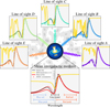 |
Fig. 1 Illustration of impact of different lines of sight in the same intrinsic spectrum. In the middle bottom panel, we show the intrinsic spectrum escaping the source (black) convolved with the mean IGM transmission at z = 3.0 (yellow). The colour line shows the convolution of the intrinsic spectrum and IGM transmission. The coloured circles show the zELDA reconstruction using the IGM-z model (discussed later). In the other five top panels, individual IGM transmission through different lines of sight are used at z = 3.0. |
2 Simulating Lyman-alpha line profiles
In this section, we detail the data sets used to produce mock Lyα line profiles that include the ISM, CGM, and IGM. In Sect. 2.1, we show the ‘shell-model’ simulations that are used based on the first zELDA version. Meanwhile, in Sect. 2.2 we detail the IGM transmission curves based on Byrohl & Gronke (2020).
2.1 Radiative transfer in the interstellar medium
As in Gurung-López et al. (2022) (hereafter ZP22), zELDA uses a set of pre-computed Lyα line profiles. These lines are computed using the Monte Carlo radiative transfer code LyaRT (Orsi et al. 2012), which performs the entire radiative-transfer computation photon by photon. This set of lines would contain the ISM radiative-transfer component, while lacking the IGM influence.
The regular grid of Lyα line profiles used in this work is the same as that described in ZP22. Basically, it consists of a five-dimensional parameter grid with 3 132 000 nodes. The five parameters are those of the thin-shell model in LyaRT. These are the outflow expansion velocity, Vexp, the neutral hydrogen column density, NH, the dust’s optical depth, τa, the intrinsic equivalent width, EWin, and the line width, Win, of the Lyα emission before entering into the thin shell. The ranges of these parameters covered by the regular grid are Vexp ∈ [0, 1000] km/s, NH ∈ [1017, 1021.5] cm−2, τa ∈ [0.0001, 0.0], EWin ∈ [0.1, 1000] Å, and Win ∈ [0.01, 6] Å. For further information on the grid specifications, we refer the reader to ZP22.
Lyα line profiles within the boundaries of zELDA’s grid are computed by 5D lineal interpolation between nodes, as described in ZP22. This leads to a typical accuracy of 0.04 in the Kolmogorov-Smirnov (KS) estimator, which is the maximum difference between cumulative distributions in the prediction of Lyα line profiles from the thin-shell model.
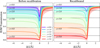 |
Fig. 2 Mean IGM transmission curves without re-calibration (left) and after re-calibration (right). Each colour shows a different redshift snapshot. The horizontal dashed black lines show the mean IGM transmission given by Faucher-Giguère et al. (2008) at z = 0,1,2,3,4,5 from top to bottom. |
2.2 Radiative transfer in the intergalactic medium
In order to include radiative transfer in the intergalactic and circumgalactic media, we made use of the transmission curves from Byrohl & Gronke (2020). These were calculated in six snapshots of the TNG100 simulation (Naiman et al. 2018; Nelson et al. 2019; Marinacci et al. 2018; Pillepich et al. 2018; Springel et al. 2018) at redshifts of 0.0, 1.0, 2.0, 3.0, 4.0, and 5.0. The Lyα radiative transfer is computed using a modified version of the code ILTIS (Behrens et al. 2019; Byrohl & Gronke 2020; Byrohl et al. 2021).The radiative transfer analysis is performed for every halo with mass greater than 5 × 10⁹ M⊙ in 1000 different line of sight. For more information, see Byrohl & Gronke (2020).
The mean IGM transmission curves of Byrohl & Gronke (2020) are shown in the left panel of Fig. 2. These show the typical structure found in the literature, on other words, a transmission close to unity redward of Lyα, a well of absorption at Lyα, and a plateau at bluer wavelengths than Lyα that decreases with redshift (Laursen et al. 2011; Gurung-López et al. 2022). The shaded regions mark the 25th and 75th percentiles. As shown by Byrohl & Gronke (2020), the scatter around the mean is significant, as there is a lot of variability in the individual lines of sight.
As mentioned above, the IGM transmission curves from Byrohl & Gronke (2020) are given in discrete redshift bins (0.0, 1.0, 2.0, 3.0, 4.0, and 5.0). However, for the training of our artificial neural networks we require a continuous redshift sampling. In order to obtain an IGM transmission curve at a given zt, we proceeded as follows. First, we obtained the target mean optical depth, τt, at zt from Faucher-Giguère et al. (2008). Next, we recalibrated the snapshot closest to zt so that its mean optical depth matches τt. For this, we used the wavelength range from −8 Å to −6 Å from Lyα. Finally, we drew a random IGM transmission curve.
The right panel of Fig. 2 shows the mean IGM transmission curves after the re-calibration. The horizontal black lines show the mean IGM transmission by Faucher-Giguère et al. (2008). Before re-calibration, we find that there is an up to 10% difference between −8 to −6 Å from Lyα. After re-calibration, by construction, both mean IGM transmissions match perfectly.
Examples of the large diversity of IGM transmission curves at different redshifts are shown throughout this work. Individual IGM transmission curves are shown as solid yellow lines in Fig. 1.
2.3 Mocking observed Lyman-α line profiles
Lyα line profiles predicted by zELDA using the LyaRT grid of line profiles and the IGM transmission curves of Byrohl & Gronke (2020) are ideal both in terms of spectral resolution and signal-to-noise ratio. In contrast, measurements of Lyα line profiles present limitations in the spectral resolution, spectral binning, and signal-to-noise ratio.
In order to produce a mock line profile of a given set of {Vexp, NH, τa, EWin, Win} and through a given IGM line of sight, we followed the next procedure. First, we produced the intrinsic Lyα line profile escaping the galaxy from the LyaRT grid as described above. Second, the spectrum after travelling through the IGM was obtained via the convolution of the ideal thin-shell Lyα line profile with the chosen IGM transmission curve. Third, we downgraded the quality of the Lyα line profile to match the desired observation configuration as in ZP22.
The quality of a Lyα line profile is determined by three parameters: (i) the signal-to-noise ratio of the peak of the Lyα line, S/Np; (ii) the wavelength resolution element in the observed frame, Wg; and (iii) the pixel size in the observed frame, ΔλPix. To downgrade the quality of the Lyα line profile, first we convolved the ideal spectrum with a Gaussian kernel of full width half maximum (FWHM) Wg. Next, we pixelated the Lyα line profile following
 (1)
(1)
The intensity of the maximum of the line profile is computed, and Gaussian white noise is added to the spectrum with an amplitude fixed by S/Np. We note that in the training set ΔλPix and Wg are independent variables. However, in order to show the results of zELDA we fixed ΔλPix = Wg/2 across all the plots and tables to reduce from three dimensions {S/Np, Wg, ΔλPix} to only two {S/Np, Wg}.
In Fig. 3, we show four spectrum quality configurations progressing from best to worst from left to right. In particular, the left column uses S/Np = 15.0 and Wg = 0.25 Å; in the middle left we have S/Np = 10.0 and Wg = 0.5 Å, in the middle right we have S/Np = 7.0; and Wg = 1.0 Å and Wg = 1.0 Å, S/Np = 7.0 can be seen in the rightmost panel. Lyα profiles are fixed at a redshift of 3.0. The intrinsic Lyα line profile emerging from the galaxy (modelled with the LyaRT grid) is shown in red, while a randomly chosen IGM transmission is shown in pink. The mock observed Lyα line is shown in black. The other coloured lines are zELDA’s reconstructions of the observed Lyα line profile that is discussed in Sect. 3. Each row shows the same outflow configuration, {Vexp, NH, τa, EWin, Win}, which is listed in Table C, through the same line of sight. In the left column (cases A, E, and I), the observed line profile closely follows the convolution of IGM and the intrinsic line profile. In particular, the pixel size is small in comparison to the size of the Lyα peaks. Also, most of the pixels with the peaks are above the noise. Meanwhile, the quality of the middle columns is worse. For example, the blue peak in E is clearly visible in the observations, while it is more difficult to see in G. Finally, the rightmost column shows the Lyα spectrum heavily affected by noise and a relatively low spectral resolution. While cases G and H are relatively well recovered given their widths, the strong absorption feature present in I is mostly removed from L. In fact, while the quality is high enough, zELDA manages to properly reconstruct the width of the Lyα line profile in I and J. Meanwhile, at K and L zELDA fails to correctly recover the width given the relatively low quality of the mock line, for which the width of the red peak starts to be comparable with the resolution and pixel size.
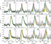 |
Fig. 3 Example of line-profile reconstruction at different line-profile qualities and using our different models. The true Lyα line before passing through the IGM is displayed in red. The IGM transmission curve is shown in pink. The true Lyα line profile is fixed in each row. The observed line profile, after IGM absorption and mocking observation conditions, is shown in black. The observation conditions are fixed in each column as Wg = 0.25 Å, S/Np = 15.0, Wg = 0.5 Å, S/Np = 10.0, Wg = 1.0 Å, S/Np = 7.0, and Wg = 2.0 Å, S/Np = 5.0 from left to right, respectively. The zELDA prediction for the models IGM+z, IGM-z, and NoIGM are displayed in blue, green, and yellow, respectively. In the bottom of each panel the KS estimation between the true Lyα line profile before the IGM absorption and zELDA prediction is displayed in colours matching the model used. |
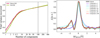 |
Fig. 4 Left: total variance recovered as function of number of principle components. We show Lyα line profiles spamming zELDA’s grid without (with) IGM absorption in red (green). The dashed black line marks the number of principal components used for the input of the artificial neural networks. We fixed the number of PCA to 100 to achieve a re-coverage of 95% of the total variance. Right: example of PCA decomposition in an IGM clean-shell model line profile. The line profiles are shown in the proxy rest frame. The original mock line profile is shown in grey. Meanwhile, the reconstructed line profiles using the N first principal components are displayed in the legend. |
3 Reconstructing attenuated Lyman-alpha emission lines
In this section, we explain our methodology to reconstruct Lyα line profiles attenuated by the intergalactic medium and estimate the Lyα IGM escape fraction. We present three models based on artificial neural networks. The idea of obtaining the redshift of a source using artificial neural networks in the Lyα line profile was initially explored in Gurung-López et al. (2021). These models are referred to as IGM+z, IGM-z, and NoIGM and have a different input and training sample. Basically, IGM+z includes the redshift of the source as input, and it is trained with a realistic IGM transmission-curve redshift evolution. The input of the IGM-z model does not include the redshift of the source, and it is trained with redshift-randomised IGM transmission curves. Finally, the input of the NoIGM model includes the redshift of the source, but no IGM transmission curve is applied to the line profiles of the training set.
This section is structured as follows. First, we detail the artificial neural network (ANN) input in Sect. 3.1, while the training sets are discussed in Sect. 3.2. Then, the ANN output is described in Sect. 3.3, and the ANN architecture is presented in Sect. 3.4. We present a feature-importance analysis in Appendix A. Finally, the parameter estimation is shown in Sect. 3.5.
3.1 Input of artificial neural networks
The input in the three presented models (IGM+z, IGM-z, and NoIGM) follows the same philosophy as those introduced in ZP22. The input consists of the line profile and its observational quality. The main difference between the models of this work and those presented in ZP22 is how the Lyα line profile is provided to the ANNs.
3.1.1 Line-profile treatment
In the IGM+z, IGM-z, and NoIGM models, we treated the observed line as follows:
The wavelength position of the global maximum of the observed line profile λmax was used as a proxy for the true Lyα wavelength λTrue. Thus, the proxy redshift is zmax = λmax/λLyα−1.
The observed line profile was moved to the proxy rest frame,
 . In particular, we converted the array where
  is evaluated in the observed frame,
  , to the rest-frame wavelength as if λTrue = λmax, i.e.,
  .
.The line profile was normalised by its maximum
 .
.The normalised line profile
 was re-binned into 600 bins from λLy α−12.0 Å to λLyα + 12.0 Å by linear interpolation between the values of
  evaluated in
  .
.The line profile was decomposed using a principal component analysis (PCA). The first 100 principal components were used as detailed below.
Steps 1 to 4 are almost identical to those in ZP22, with only minor changes in the wavelength range used. The PCA analysis is a new addition to zELDA.
In Fig. 4, we show the total explained variance as a function of the number of principal components of the training set (with varying outflow and spectral-quality properties). We present two PCA models, one for lines without IGM (red, used for the NoIGM model) and another for lines with IGM absorption (green, used for the IGM+z and IGM-z models). We find that both PCA models exhibit the same behaviour. The total explained variance grows rapidly with the first ∼7 components up to ∼90%. After a knee, the total recovered variance grows slowly, reaching ∼95% at 100 and ∼98% at 400 principal components. Below 25 principal components, the total explained variance in the lines without the IGM is greater than those including the IGM for a fixed value of principal components. This seems reasonable since the IGM absorption would add complexity to the observed Lyα line profiles. From 25 principal components onward, the total variance in both models is roughly the same.
We used the first 100 principal components in the models presented in this work. We also trained our models using only 10, 25, 50, and 75 components. We found that the accuracy of the models increased up to including the first 100 PCA components. We tested that the accuracy in all the outflow parameters kept increasing up to including the first 100 principal components as the input of our neural networks. Additionally, we tested that using the first 200 and 400 principal components did not increase the precision further when reconstructing the intrinsic Lyα line profiles.
The right panel of Fig. 4 shows an example of the PCA decomposition of a shell model line profile that is unobscured by the IGM (grey). The different coloured lines show the PCA decomposition using only the first 1, 2, 5, 10, 20, 50, and 100 components (from purple to red). The first two components focus on the red peak. The blue peak is progressively recovered as we increase the components from 3 to 20. The first 20 principal components give an accurate, although smoothed, version of the original line profile. Meanwhile, from the 20th up to the 100th components, small features are captured, including the noise pattern. Although not displayed here, the IGMs featured are encapsulated from the 20th to the 100th principal components.
3.1.2 Line profile quality and redshift
As in ZP22, we include the line profile quality as features in the input of the artificial neural networks. In particular, we include the wavelength element of resolution and the pixel size, both in the observed frame. This is the same in all three models.
Then, in ZP22 we included the redshift of the sources through the proxy zmax. In this work, we did the same in IGM+z and NoIGM. Meanwhile, the redshift was excluded from IGM-z. On one hand, the motivation behind IGM+z is to produce a model with the same IGM distribution as in Byrohl & Gronke (2020). On the other hand, the goal behind IGM-z is to provide a model that is as unbiased as possible by the redshift-dependent quantities and that matches the mean IGM transmission of Faucher-Giguère et al. (2008).
3.1.3 Total input
The input for each model is slightly different. The models IGM+z and NoIGM use 103 features:
– Input = [… 100 PCA …, Wg, Δλpix, zmax].
However, the PCA model used for IGM+z includes the IGM absorption, while the PCA model used for NoIGM does not. Next, the input for the IGM-z model is the same as before, but excluding zmax, i.e., 102 features:
– Input = [… 100 PCA …, Wg, Δλpix],
where the PCA model is the same as in IGM+z and includes the IGM absorption.
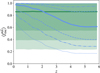 |
Fig. 5
|


3.2 Training sets of artificial neural networks
The training sets for IGM+z, IGM-z and NoIGM are different from each other. Nevertheless, they share the same number of Lyα line profiles (4.5 × 10⁶), and the outflow parameters {Vexp, NH, τa, EWin, Win} are equally homogeneously and randomly drawn from the space covered by the LyaRT grid. The mock Lyα line profiles uniformly cover from Win = 0.01 Å to 4.0 Å, ΔλPix = 0.01 Å to 2.0 Å, and from S/Np = 5.0 to S/Np = 15.0. We tested that for this training set size, our artificial neural networks have converged. In addition, for the three models, redshifts from zero to six were homogeneously sampled. We highlight that the IGM transmission curves from Byrohl & Gronke (2020) are computed up to the snapshot at z = 5. Therefore, the predictions given by IGM+z and IGM-z at z > 5 should be considered with caution. The particularities of the training sets, therefore, depend on how the IGM is treated. Details for each set are listed below.
IGM+z: This training set includes line profiles with the IGM absorption. In this model, we use the uncalibrated IGM transmission curves. In particular, the IGM transmission curve to each Lyα line profile uses the actual redshift of the source. Therefore, there is an evolution in the IGM where Lyα line profiles at higher redshift are more attenuated.
IGM-z: This training set also includes line profiles with the IGM absorption. However, in contrast to IGM+z, we use the re-calibrated transmission curves, which are drawn randomly, irrespective of the source redshift. Thus, the IGM absorption distribution is constant with redshift. There will be Lyα that is basically unabsorbed (typical of z = 0) and some that are absorbed significantly (typical of high z) at all redshifts.
NoIGM: This training set does not use IGM transmission curves.
In Fig. 5, we compare the distribution of  (IGM Lyα escape fraction ± 2 Å around Lyα) as a function of redshift in the training sets for the IGM+z (blue) and IGM-z (green). The model IGM+z exhibits an evolution in the median
  as a function of the redshift, given by the evolution of the opacity of IGM. At z < 1, the median
  is close to 1.0, while at z > 4.0 it stalls at 0.6. In particular, there is no evolution from z = 5.0 to z = 6.0, as the last snapshot with IGM transmission curves is at z = 5.0. Meanwhile, at z < 0.5 the training set for IGM+z shows less scatter than at high redshift, exhibiting more than 98% of the sample with
  > 0.6. Then, at higher redshift the scatter increases, and at z = 4 as 98% of the sample is between 1.0 and 0.2. Then, focusing on IGM-z, as the redshift of the IGM transmission curve is randomised, there is no evolution in the distribution of
  as a redshift function. The IGM-z model is conceived as a ‘redshift-unbiased’ model.
The IGM+z and IGM-z models have the same overall aim: to reconstruct an IGM-attenuated Lyα line profile and obtain the IGM escape fraction. IGM+z and IGM-z are complementary to each other. In machine learning, the input features and the training set are very important for the output of the neural networks. If a training set exhibits some particular biases, the output can potentially show the same biases. In principle, IGM+z uses in the input the proxy redshift of the source and the evolution of the IGM transmission curves with redshift of the TNG100 simulation Byrohl & Gronke (2020). Furthermore, in Appendix A we performed a feature-importance analysis on IGM+z, IGM-z, and NoIGM, finding that the input proxy redshift had a strong influence in the determination of the outflow parameters and especially in  . Thus, the output of IGM+z can potentially be biased towards the IGM redshift evolution in Byrohl & Gronke (2020). For these reasons, we developed IGM-z, which does not include the proxy redshift in the input and has no IGM redshift evolution in the training set. Thus, IGM-z should be a redshift-unbiased model. In the following sections, we compare the results obtained by IGM+z and IGM-z, finding that both perform really similarly with only small differences at z < 1. Finally, we remark that if a redshift-dependent evolution (e.g. on Vexp or
  ), is found by both IGM+z and IGM-z, would give robustness to the result.
On the other hand, the motivation behind NoIGM is to show a fit that lacks the IGM component. Thus, the predicted Lyα line profile and that observed will always resemble each other, whether the observed line is IGM attenuated or not. NoIGM is useful for understanding possible biases of neglecting the IGM component in observed Lyα line profiles. Additionally, if the models with IGM attenuation (IGM+z and IGM-z) and NoIGM predict the same line profile, that line is probably not IGM absorbed, relatively speaking.
3.3 Output of artificial neural networks
The three models – IGM+z, IGM-z and NoIGM – have a similar output, almost akin to that of the ANN in ZP22. As in ZP22, there are five output variables associated with the outflow configuration {Vexp, NH, τa, EWin, Win}. In order to estimate the redshift of the source, another output is the difference between the wavelength set as Lyα and the true Lyα wavelength in the proxy rest frame, ΔλTrue. The true Lyα wavelength in the observed frame,  , can be recovered as
 (2)
(2)
Then, the redshift of the source is  . For further details, see Gurung-López et al. (2022).
In the case of IGM+z, IGM-z, we included additional variables. In each of the Lyα line profiles used for the training set, we measured the fraction of photons that escape the IGM in wavelength intervals centred around Lyα lines. We refer to these variables as  , where x is the width of the wavelength window in the rest frame used. For example,
  is the Lyα IGM escape fraction in λLy α ± 2 Å in rest frame. zELDA’s IGM+z and IGM-z models include wavelength windows from 1 Å to 10 Å. We find that for a wavelength window of 4 Å the Lyα IGM escape fraction converge. Increasing the window size does not increase
  . Also, up to a wavelength window of 4 Å the escape fraction increases with window size. This is reasonable since the mean IGM transmission curves show a drop close to the centre of the Lyα line; then, they stabilise at the cosmic mean IGM transmission.
3.4 Architecture of artificial neural networks
For each output property, we trained an independent ANN. We tested different configurations. We found that for {Vexp, NH, τa, EWin, Win} and  the best configuration is a three-layer ANN with sizes 103, 53, and 25. Meanwhile, for ΔλTrue we found that a nine-layer ANN had the best accuracy with sizes 103, 90, 80, 70, 60, 50, 40, 30, and 20.
We describe a feature-importance analysis in Appendix A. Overall, we find that the ± 4 Å region around the Lyα wavelength contains the most important information for most predicted shell parameters.
3.5 Redshift, outflow, and IGM escape fraction estimation
The shell properties Vexp, NH, τa, EWin, Win and the IGM escape fractions  and ΔλTrue are obtained as the median of the distribution of outputs resulting from the ANN using 1000 perturbations of the original observed Lyα line profile as input by its noise pattern (as in Gurung-López et al. 2022). The 16th and 84th percentiles are used as the 1σ uncertainty of these properties. In ZP22, we demonstrated that this methodology achieves better accuracy compared to directly using the ANN output of a single realisation. Additionally, making multiple iterations provides the uncertainty for the measurement. This is further discussed in Appendix B.
4 Results on mock Lyman-α line profiles
In this section, we show the results of the three ANN models presented in this work on mock observed Lyα line profiles. First, we characterise the accuracy in reconstructing the line profiles in Sect. 4.1. Then, we show the performance of zELDA in recovering the evolution of the IGM escape fraction through time in Sect. 4.2. Finally, we provide an analysis of zELDA’s capability to reconstruct the intrinsic stack spectrum emerging from galaxies and before the IGM radiative transfer in Appendix F.
In this section, we highlight how we made use of mock Lyα spectra generated using the same techniques as those of the training set. However, the spectrum analysed in this section is not the same as that in the training and validation sets of our models. In fact, as discussed below, we changed the  , redshift, and output parameters distributions in comparison with the training set to test the model’s performance and possible biases.
4.1 Accuracy of the ANN models
Here, we characterise the accuracy of IGM+z, IGM-z, and NoIGM in recovering the redshift, outflow parameters, and Lyα IGM escape fraction. First, we show some individual examples. Further details on the accuracy of each parameter are given in Appendix C. Moreover, we show the precision in the recovered line profile shape in Appendix E.
In Fig. D.1, we display 20 individual mock line profiles that were successfully reconstructed (low Kolmogórov-Smirnov estimator values) by the zELDA, IGM+z and IGM-z models. In each panel, the intrinsic Lyα line profile leaving the galaxy is shown in red, while the IGM transmission curve is shown in pink. The mock observed Lyα line profiles used to build the input for the ANN models are shown in black. The quality of the mock line profiles is S/Np = 15.0, Wg is 0.1(1 + z) so that the resolution element is constant in the rest frame, and ΔλPix = Wg/2. zELDA’s prediction using IGM+z, IGM-z and NoIGM are displayed in blue, green, and yellow, respectively. The true  is shown in black, while the predictions of IGM+z and IGM-z are given at the top in blue and at the bottom in green, respectively, with their 1σ uncertainty. Kolmogorov-Smirnov is shown for IGM+z, IGM-z and NoIGM, from left to right, between the predicted line and the intrinsic one (red).
Lyα line profiles in Fig. D.1 are typically reconstructed by IGM+z, IGM-z with KS < 0.1. Both the red peak and the blue peak are properly recovered at the same time. For example, in cases E and I the observed Lyα line profiles still show some hints of the existence of a blue peak prior to the IGM. IGM+z and IGM-z reconstruct the intrinsic blue peak quite well. However, despite the general good reconstruction of the blue peaks, IGM+z and IGM-z sometimes underpredict the blue peaks (case S). This tends to happen when the IGM absorption is so strong that most of the blue peak information is erased from the observed spectrum. However, it is remarkable that even in some scenarios of heavy IGM attenuation, both the blue and red peaks are properly reconstructed (cases J, N, O, P and R). Moreover, in some extreme cases where half or more of the line is obscured (cases P, Q, S and T), the Lyα line profiles are reconstructed with typical KS < 0.8.
Meanwhile, NoIGM works relatively well at low redshift (cases A, B, C). However, NoIGM fails to recover the intrinsic Lyα line profiles of the heavily attenuated observed Lyα line profiles. In fact, the red peaks are relatively well fitted, while the blue peaks are poorly reconstructed (cases L, M, P, R, S). There are some cases in which NoIGM fails to reconstruct the red peak of the line (cases Q, T) as well.
The examples in Fig. D.1 demonstrate two key aspects of the Lyα line profile reconstruction. First, Fig. D.1 shows that in some cases, the IGM attenuation can reshape a thin-shell Lyα line profile into another Lyα line profile similar to another thin-shell configuration. This is made evident when comparing the NoIGM output to the observed lines in cases K, L, M, N, R, and S. Second, we note that – especially in examples K, L and N – the red peak of the observed line profile is well fitted by the three models, including NoIGM. NoIGM gives a different prediction for the blue peak than IGM+z and IGM-z. This shows that the observed red peak degenerates with the intrinsic blue peak. These two facts result in perhaps inevitable confusion in the reconstructed shell parameters, redshift, and Lyα IGM escape fraction for some observed Lyα line profiles.
Figure D.2 shows some cases where the line profile reconstruction by IGM+z, IGM-z could be considered deficient or improvable (KS>0.1). The colour code follows Fig. D.1. In general, we find that IGM+z and IGM-z succeed or fail in the same line profiles. Only in a few cases does IGM+z or IGM-z accurately recover the intrinsic line (e.g. KS=0.04), and the other IGM model gives an inaccurate reconstruction (e.g. KS=0.2). IGM+z and IGM-z tend to give worse predictions when the observed line after IGM absorption resembles that of a wrong outflow model (here, especially in cases A and D). Another source of inaccuracy is the complete destruction of the blue-side information, leading to an over- or under-prediction of the Lyα blue peak (cases F and G). In general, we also find that the NoIGM model does not recover the correct intrinsic line profile when IGM+z and IGM-z do.
We studied the ratio between successful and unsuccessful reconstructions. For simplicity, we used KS = 0.1 as a threshold to distinguish between successful and unsuccessful reconstructions. We find that the fraction of sources with KS < 0.1 (properly recovered) depends on the quality of the Lyα line profile. The better the spectral quality, the higher the fraction of sources with KS < 0.1. Taking into account IGM+z and IGM-z, the fraction for sources with KS < 0.1 is greater than 90% for many of the quality configurations explored. We find that a good fraction of the line profiles are properly recovered, even at relatively bad spectral quality. In particular, we find that for S/Np > 7.5 and  > 0.5 there is a typical value of Q(KS = 0.1) > 70%, even at Wg = 4.0 Å. More details can be found in Appendix E. In particular, we find that zELDA reconstructs the galactic component successfully for 95% of the cases for HST/COS-like spectral quality and 80% for MUSE-WIDE-like spectral quality.
4.2 Reconstructing the IGM escape fraction evolution
In this section we explore zELDA’s capability in measuring the  evolution through cosmic time. For this purpose, we developed mock samples of Lyα line profiles with different IGM escape-fraction redshift relations and analysed zELDA’s performance on these mocks.
4.2.1 Mean Lyα IGM escape-fraction redshift-dependence reconstruction
In this section, we study the capabilities of zELDA in reconstructing the redshift evolution of the mean  . For this goal, we developed Lyα line-profile mock samples with different mean
  evolution. Later, we studied the accuracy of IGM+z and IGM-z in these mocks.
We parameterised the mean  redshift dependence as a Fermi-Dirac distribution:
 (3)
(3)
where a and b are two free parameters. The Fermi-Dirac distribution was chosen to reproduce the expected average evolution from an opaque (f=0.0) to transparent IGM (f=1.0) with an asymptotic behaviour on both ends.
For a given combination of parameters a and b, we generated a set of 500 Lyα line profiles homogeneously distributed from z = 0 to 6. Each Lyα line profile at redshift z1 was assigned an IGM transmission curve at a random redshift z2. Next, the outflow line profile (intrinsic) was convolved with the chosen IGM transmission curve, and  was measured. If the computed
  was within 10% of the ⟨
 (z1), this Lyα line profile was accepted as valid. However, if this condition was not met, a new IGM transmission curve at another random redshift z3 was assigned until the condition was fulfilled. By construction, all Lyα line profiles will exhibit
  alues close to the Fermi-Dirac with parameters a and b.
We produced Lyα line-profile mocks for four a and b combinations that populate the  −z space. In Figs. 6 and 7, we show four {a, b} combinations, which are Mock1 {7.0, 0.7} (green), Mock2 {6.0, 0.6} (red), Mock3 {5.0, 0.5} (blue), and Mock4 {4.0, 0.4} (grey). For each a and b combination, we produced mocks with six spectral quality configurations. For S/Np = 10.0 (top row) and S/Np = 15.0 (bottom row), three values of Wg were run: 0.1 Å, 1.0 Å, and 2.0 Å from left to right. The solid coloured lines show the parametric
  . and the coloured squares the actual
  in that redshift bin.
In Fig. 6, we show the IGM+z prediction for the mock samples. The coloured crosses show the  predictions line per line. The coloured circles mark IGM+z’s estimations of
  in the same redshift bins as for the true values. Meanwhile, the results for IGM-z are shown in Fig. 7. In general, we find that both IGM+z and IGM-z recover the
  evolution with redshift. For both models, the precision of the reconstructed
  . evolution changes with the spectral quality. For lines with higher resolution and S/Np, the recovered
  follows the true
  evolution well. However, when the spectral quality decreases, some biases appear in the
  estimate. We also find that IGM+z and IGM-z show a limitation for low
  values (∼0.4). For example, at S/Np = 15.0 and Wg = 0.1 Å,
 . stales at ∼0.45 at a redshift of ∼5 in Mock4, while it should fall down to 0.3. Also, for the worst spectral quality configuration (Wg = 2.0 Å) we find that, while the general
  redshift evolution is recovered,
  is slightly biased for Mock1 and Mock4. In particular, the results in Mock1 are up to ∼10% under-predicted, while those for Mock4 are up to ∼10% over-predicted. Meanwhile, the results for Mock2 and Mock3 for Wg = 2.0 Å are quite unbiased, and most individual measurements are 1σ compatible with the true values.
We find that while the S/Np of the line has an impact on the accuracy of the recovered  , Wg has a greater influence. This is also found when determining
  in individual line profiles. As shown in Fig. C.3, focusing on the
  ∈ [0.95, 1.0] regime, for Wg = 0.1 Å (HST-like quality) changing S/Np from 15.0 to 5.0 produces a drop in
  accuracy from 0.03 to 0.04. However, for S/Np = 10.0, the
  accuracy at Wg = 0.25 Å is 0.03, while at Wg = 2.0 Å it is 0.1 (MUSE-WIDE-like quality). This becomes even more apparent in the
  ∈ [0.65, 0.8], where there is no clear
  accuracy dependence on S/Np, while it gets worse for larger Wg values.
In general, Fig. 6 shows that the IGM+z model provides an accurate  estimation for the explored mocks at Wg = 0.1 Å, as most of the measurements are 1σ compatible with the true values. Moreover, IGM+z provides a relatively unbiased and accurate prediction between redshifts 2 and 5 for the four mocks presented and for all spectral-quality configurations. However, we find that the IGM+z model is biased at z < 1 at every explored spectral quality (e.g. Mock3 and Mock4). IGM+z tends to over-predict
  and gives values close to unity at this redshift range. This bias becomes stronger as the spectral quality decreases. For example, at z = 1 and Wg = 0.1 Å,
  is over-predicted by ∼10%. Nevertheless, the general trend (
 decreases with z) is recovered in all spectral-quality configurations and redshift bins.
Focusing on IGM-z (Fig. 7),  is nicely recovered for Wg = 0.1 Å and S/Np = 10.0 and S/Np = 15.0 for the explored evolution cases. Also, we find that IGM-z is less biased towards
  . than IGM+z at low redshift. For example, at Wg = 0.1 Å the
  evolution in Mock4 is recovered almost perfectly with no apparent bias at z < 1. For Wg = 1.0 Å,
  is overestimated by 10% for Mock4 at z < 1. Moreover, unlike for IGM+z, at z < 1 the rank order in
  is recovered properly. Individual measurements of Mock1 are greater than those of Mock2, which are greater than those of Mock3, which are above those of Mock4. Furthermore, at z > 1 we find the same trends as in IGM+z.
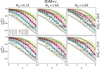 |
Fig. 6 zELDA’s prediction of mean |


4.3 Stacked line-profile reconstruction
In this section, we explore zELDA’s ability to reconstruct the stack (or average) of intrinsic Lyα line profiles. Our focus here is to study whether zELDA is able to measure the evolution or non-evolution of the intrinsic stacked Lyα line profile. For this goal, we used mock samples of the Lyα line profiles. Meanwhile, a detailed analysis for individual spectral recovery can be found in Appendix E.
Outflow parameters in redshift nodes used for the Lyα-line-profile stacked mocks.
Given a sample of Lyα line profiles with a given redshift distribution, we followed the procedure described below in order to compute the stack line profile. First, we run zELDA (IGM+z, IGM-z or NoIGM) in order to obtain the redshift of the Lyα line profile by running our ANN. Next, we move all observed Lyα line profiles to a common wavelength array in the rest frame using the redshift provided by zELDA. Every Lyα line profile is normalised so that the their maximum reaches unity. Finally, the stacked Lyα line profile is computed as the median flux in each wavelength bin.
We present two types of samples of mock Lyα line profiles. In the first one, Mock_Evo, the intrinsic Lyα line profiles change with redshift. In particular, for a given Lyα line profile at redshift zt, the outflow properties are linearly interpolated from the z nodes listed in Table 1. For illustration, in each node, the outflow parameter combination is chosen so that the intrinsic line profile changed dramatically from node to node. There is no physical motivation behind the chosen outflow parameters. The goal of Mock_Evo is to test if zELDA manages to retrieve an evolving intrinsic stack Lyα line profile. At the same time, Mock_Evo is a good scenario in which to test whether our ANN models are biased towards outputting the average spectrum in the training sets. If zELDA retrieved the same stacked spectrum independently of the intrinsic average spectrum, zELDA would be biased. As shown next, zELDA models are not biased towards the average spectrum of the training set. The top left panel of Fig. 8 shows the stacked Lyα line profile at a redshift between 0.75 and 1.25 (grey), between 1.75 and 2.25 (blue), between 2.75 and 3.25 (green), between 3.75 and 4.25 (yellow) and between 4.75 and 5.25 (red).
In the second mock sample, Mock_fix, all the line profiles use the same outflow parameters: Vexp = 200.0 km s−1, NH = 19.3 cm−2, EWin 20.0 Å, Win 2.0 Å and τa = 0.001. These were chosen so that the intrinsic line profile resembled the observed Lyα line profiles’ stack at low redshift (Hayes et al. 2023). The top left panel of Fig. F.1 shows this outflow line profile.
The Mock_Evo-observed stacked Lyα line profile after including the IGM is shown in the top right panels of Fig. 8 for two spectral-quality combinations: S/Np=15 and Wg = 0.1 Å (top) and S/Np = 10 and Wg = 2.0 Å (bottom). For both spectral-quality configurations, the higher the redshift, the more attenuated the blue side of Lyα. Meanwhile, the red side of Lyα remains unabsorbed. This is a direct consequence of the redshift dependence and shape of the mean IGM transmission curves (shown in Fig. 2). For instance, the intrinsic stacked line profile at z ∼ 1 remains mostly unchanged after applying the IGM absorption. Furthermore, the stacked line profile at z ∼ 5 intrinsically exhibits a relatively strong blue continuum and a faint blue peak. These features are erased from the observed stack spectrum as a result of the IGM absorption. In the same way, the strong blue peak in the intrinsic stack at z ∼ 4 is also erased.
At the same time, the Mock_fix-observed stacked Lyα line profile after including the IGM (top right panels of Fig. F.1) shows the same trends as that of Mock_Evo. We find that the higher the redshift, the more absorbed the blue side of Lyα. In particular, at z ∼ 4 the blue peak is erased. In addition, spectral quality has an impact on the observed stack spectrum of Lyα. As Wg is fixed in the observed frame, the resolution element in the rest frame is smaller for sources at higher redshifts. This means that, for S/Np = 10.0 and Wg = 2.0 Å, the Lyα stack spectrum at z ∼ 1 is wider than at z ∼ 5.
We present the results for the stacked Lyα line profile reconstruction in Fig. 8 for the redshift-dependent Lyα line profile (Mock_Evo). In order to compute the reconstructed intrinsic Lyα line profiles, we ran zELDA in each individual observed line profile. Next, we followed the same procedure for computing the stacked line profile described earlier. The stacked Lyα line profiles reconstructed by IGM+z, IGM-z, and NoIGM are shown in the bottom columns from left to right. The top row shows S/Np = 15.0 and Wg = 0.1 Å (HST-like quality), while the bottom shows S/Np = 10.0 and Wg = 2.0 Å (MUSE-WIDE-like quality). The accuracy of the reconstruction is quantified by the KS estimator between the intrinsic stack and the reconstructed one, which are shown within each panel.
In general, the three ANN models show that there is a clear evolution in the Lyα stacked line profile. We find that, in general, IGM+z and IGM-z manage to reconstruct the intrinsic stacked Lyα line profile accurately with typical values below KS = 0.1. In particular, the stack is more accurate for the S/Np = 15.0 and Wg = 0.1 Å configuration typically with KS < 0.06. For example, both IGM+z and IGM-z recover the blue peaks visible in the intrinsic stack at z ∼ 3, 4, and 5. Even the small hint of a blue peak present in the z ∼ 2 bin is recovered. However, the reconstruction in the blue peaks is not perfect. For example, in the z ∼ 4 stack, the reconstructed blue peak is slightly under-predicted. It is also noticeable that the amplitude of the continuum blue-side Lyα line profile is relatively well recovered.
The NoIGM model recovers the intrinsic Lyα line profile well at z ∼ 1, with KS = 0.05. However, at z > 1, the stack is poorly constrained, with typical KS values greater than 0.1. For example, the NoIGM ANN provides reconstructed Lyα line profiles that exhibit the same blue continuum as the observed stacked line profile. In addition, the blue peaks of the high-redshift bins were not recovered.
In Fig. F.1, we show zELDA’s prediction for the static Lyα line-profile sample (Mock_fix). In general, we find the same trends as in Mock_Evo. Both the IGM+z and IGM-z models recover the non-evolution of the stacked Lyα line profile accurately. The stacked line profile is better reconstructed for better spectral quality. Typically KS < 0.10 for S/Np = 10.0 with Wg = 2.0 Å and KS < 0.05 for S/Np = 15.0 with Wg = 0.1 Å. The blue peak is reconstructed at all redshifts, although with slightly different amplitudes. Meanwhile, NoIGM does not manage to recover the non-evolution. NoIGM correctly predicts the stacked line profile at z ∼ 1 with KS = 0.02 for S/Np = 15.0 with Wg = 0.1 Å. However, at z > 1.0 does not recover the existence of the blue peak.
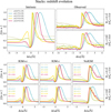 |
Fig. 8 Stacked line-profile reconstruction example in mock Lyα line profiles using the Lyα line profiles with redshift dependence. The stacked line profile is shown the redshift intervals [0.75,1.25] (grey), [1.75,2.25] (blue), [2.75,3.25] (green), [3.75,4.25] (yellow), and [4.75,5.25] (red). The Lyα stacked line profiles using the Lyα line profiles before applying the IGM absorption are displayed in the top left panel. The two top right panels display the Lyα stacked line profile after applying the IGM absorption and mocking observation qualities similar to those of HST (Wg=0.1 Å and S/Np = 15.0, top) and MUSE (Wg = 2.0 Å and S/Np = 10.0, bottom). The six bottom panels show the reconstructed stacked Lyα line profiles. Each bottom column makes use of a different ANN model: IGM+z, IGM-z, and NoIGM from left to right. The KS between the stacked Lyα line profile before the IGM (left column) and that of the reconstructed Lyα line profiles is displayed in coloured text matching the redshift bin. |
5 Summary and conclusions
The observed Lyα line profile is shaped by the complex radiative transfer taking place inside the galaxies in the interstellar medium, in the circumgalactic medium after escaping the galaxy, and in the intergalactic medium. In this paper, we present the second version of the open source code zELDA. The second version of zELDA focuses on disentangling the ISM and IGM contributions to the Lyα line profile using artificial neural networks. zELDA is publicly available3 along with installation and usage tutorials4.
Our training sets contain mock Lyα line profiles with ISM and IGM attenuation mimicking a wide range of observed spectral quality configurations. The ISM contributions come directly from the first version of zELDA ZP22, which counted with a grid of precomputed shell-model line profiles using a Lyα Monte Carlo radiative transfer (LyaRT Orsi et al. 2012). Meanwhile, the IGM attenuation comes from the Lyα transmission curves published by Byrohl & Gronke (2020). These were obtained by running a Monte Carlo Lyα radiative transfer code (a modified version of ILTIS, Behrens et al. 2019) in the TNG100 simulation (Nelson et al. 2019), at six snapshots between redshifts of 0.0 and 5.0.
We present three ANN models. All include the first 100 components of the PCA decomposition of the observed Lyα line profile and spectral quality. First, IGM+z includes a proxy redshift of the sources and the IGM transmission lines assigned to the sources in the training are at the redshift of the source. Meanwhile, IGM-z does not include the redshift of the source in the input, and sources are assigned random IGM transmission curves. Finally, for comparison we develop the model NoIGM, which includes a proxy redshift of the source in the input but the Lyα line profiles in the training set lack the IGM contribution.
zELDA’s performance on a mock Lyα line profile can be summarised as follows:
We tested our ANN models in mock Lyα line profiles. We find that IGM+z and IGM-z manage to reconstruct the shape of the Lyα line profile emerging from the ISM. The accuracy of the reconstruction depends on the spectral quality of the observed line profile. For example, for the typical spectral quality of Lyα line profiles obtained by the Cosmic Origins Spectrograph (COS Green et al. 2012) on board the Hubble Space Telescope, 95% of the Lyα line profiles should be recovered with a Kolmogórov-Smirnov estimator below 0.1. Meanwhile, for data with the spectral quality of the MUSE-WIDE survey (Urrutia et al. 2019; Herenz et al. 2017), 81% of the Lyα line profiles are typically reconstructed with a KS<0.1;
Additionally, we tested zELDA’s ability to reconstruct the stacked line profile of the line emerging from the ISM of the IGM’s attenuated line profiles. We find that the Lyα stacked line profile can be recovered with KS<0.7 for HST-and MUSE-like data by both IGM+z and IGM-z. Moreover, the precision in the stack reconstruction enables us to detect evolution or non-evolution in the ISM stacked line profile;
Interestingly, zELDA is capable of predicting the IGM Lyα escape fraction,
 , with an uncertainty of ∼0.03 in HST-like data and ∼0.12 for MUSE-like data. In fact, we found that IGM+z and IGM-z are able to detect evolution in
  from redshift 2.0 onward for MUSE-like data. Meanwhile, IGM+z provides
  values biased towards 1 at z<1.0. In contrast, IGM-z seems unbiased in this redshift range.
 at
at  < 0.5 or reconstructing the shape of Lyα line profiles with
  < 0.4. Nevertheless, this work demonstrates that disentangling the ISM from the IGM contributions is possible at the level of individual Lyα line profiles. This opens multiple scientific pathways. Some examples of the many possible applications of zELDA to observed data are listed as follows:
The exploration of what shapes the ISM’s emerging Lyα line profiles in high-redshift galaxies. This could be done by correlating the inferred ‘shell model’ parameters with the luminosity of their spectral features or galaxy properties such as mass, neutral hydrogen column density, and so on;
There is still some debate as to whether the IGM large-scale properties affect the visibility of Lyα. A spectroscopic survey covering a large enough area and using zELDA could directly measure if there is an excess of clustering signal in
 with respect that of LAEs.
Reconstructing the galactic line profile can give insight into gas properties of high-z galaxies, and, in particular, it can be used to infer the escape fraction of ionising photons, for example (e.g. Saxena et al. 2024);
Distinguishing between the galactic and the IGM contribution to the Lyα line shape can also help to constrain HI morphology on larger scales. Specifically, from the (non)visbility of blue peaks one can infer HII regions (‘bubble sizes’) during the epoch of re-ionisation (see e.g. Mason & Gronke 2020). We plan to expand zELDA in this direction in future work;
A more minor application of zELDA could be correcting measured Lyα luminosity functions (LFs). Currently, Lyα LFs are measured with the observed Lyα luminosity, which is attenuated by the IGM. zELDA provides a source-by-source
 . Therefore, zELDA can provide the Lyα LF for star forming sources before IGM attenuation. This could shed light on the cosmic star formation history at high redshift.
Acknowledgements
The authors acknowledge the financial support from the MICIU with funding from the European Union NextGenerationEU and Generalitat Valenciana in the call Programa de Planes Complementarios de I+D+i (PRTR 2022) Project (VAL-JPAS), reference ASFAE/2022/025. This work is part of the research Project PID2023-149420NB-I00 funded by MICIU/AEI/10.13039/501100011033 and by ERDF/EU. This work is also supported by the project of excellence PROMETEO CIPROM/2023/21 of the Conselleria de Educación, Universidades y Empleo (Generalitat Valenciana). MG thanks the Max Planck Society for support through the Max Planck Research Group. DS acknowledges the support by the Tsinghua Shui Mu Scholarship, funding of the National Key R&D Program of China (grant no. 2023YFA1605600), the science research grants from the China Manned Space Project with no. CMS-CSST2021-A05, and the Tsinghua University Initiative Scientific Research Program (no. 20223080023). This research made use of matplotlib, a Python library for publication quality graphics (Hunter 2007), NumPy (Harris et al. 2020) and SciPy (Virtanen et al. 2020).
Appendix A Feature importance analysis
The feature importance analysis of the spectral features is made by shuffling the fluxes in wavelength bins of 1 Å in the rest frame of the sources, as in ZP22. Next, we convert the altered spectrum with the PCA model and pass it to the ANN along with the actual Wg, ΔλPix and zmax values. Then, in order to compute the importance of Wg, ΔλPix and zmax, we shuffled these properties one by one. The importance is computed as I = σoriginal/σshuffled−1, where σoriginal is the accuracy of the ANN predicting a given output variable and σshuffled is that but using the perturbed input. In general, σshuffled < σOriginal, since the input without perturbation contains more information. Therefore, I > 0, in general.
In Fig. A.1 we show the feature importance analysis of ΔλTrue, Vexp, NH, EWin, Win and  for the IGM+z model with Wg = 0.25 Å, ΔλPix = 0.125 Å and S/Np = 15.0. The general trends found here are also present for other quality configurations and IGM-z and NoIGM. We find the same general trends as in ZP22. For ΔλTrue, Vexp, NH, Win and
  the regions closer than 5 Å contains the most information. This tends to be skewed redwards Lyα in the three models. However, the models including IGM, IGM+z and IGM-z, give more importance to redder wavelengths than NoIGM. This shows that IGM+z and IGM-z ‘trust’ more the red side of Lyα. This makes sense considering that the blue side of Lyα could be heavily influence by the IGM. Still, some information in the blue side is being used in order to estimate the output. The ANN constraining EWin gives the most importance to the region +5 Å from Lyα, which should be dominated by the continuum of the source. In particular, the ANN constraining ΔλTrue exhibits the narrowest importance peak around Lyα (± 1 Å). Finally, focusing in
  , we find that in the IGM+z model, the importance of zmax is 0.38, which shows that it plays a significant role in determining
  . Actually,
  is variable for which zmax is the most informative.
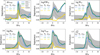 |
Fig. A.1 Feature importance analysis for the IGM+z (blue), IGM-z (green) and NoIGM (yellow). For comparison, the stacked line profiles with its 1σ scatter is shown in grey. Each subplot shows the importance determining a different property. In top row, ΔλTrue, EWin, Win from left to right. In the bottom row, NH, Vexp, |

Appendix B Individual parameters uncertainty estimation
In ZP22 we found that the uncertainty computed through this methodology had less than a 10% error, and therefore needed no correction. However, we find that the models presented in this work tend to underestimate the uncertainty in the output parameters. In the top panels of Fig. B.1 we show the comparison between the fraction of cases that a measurement is in compatible with the intrinsic true value, fcomp, as a function of the confidence level. Each subplot shows the indicated outflow property. Ideally this relation should follow perfectly a 1:1 trend. Focusing in NoIGM (yellow) we find that before correction (solid line) the uncertainty is underestimated no more than 10%, except for τa, as it was the case in ZP22, which did not include IGM. We find that the uncertainty in the outflow parameters can be underestimated up a 20% in IGM+z and IGM-z. This bias in the uncertainty estimation is produced by the IGM inclusion. Some IGM transmission curve can produce observed Lyα line really close to unabsorbed thin shell spectrum. In some of these cases the outflow parameters predicted correspond to the ‘fake’ thin shell spectrum rather than the intrinsic one. This causes than in smaller fraction of cases the true outflow parameters and the predicted ones are compatible at a given confidence level than in NoIGM. We correct our uncertainty estimation so that fcomp and the confidence level follow a 1:1 relation. The correction factors depend on the confidence level and are shown in the bottom panels. fcomp as a function of the confidence level after the correction is shown in dots.
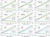 |
Fig. B.1 Top: Comparison between the fraction of cases that a measurement is in agreement with the intrinsic true value, fcomp, as a function of the confidence level. Bottom: Applied correction factor to uncertainty. The uncorrected fcomp is shown in colored solid lines, which IGM+z in green, IGM-z in blue and NoIGM in yellow. fcomp after the correction is shown in colored dots. In each panel a different output property is shown. In the first row zmax, Vexp and NH from left to right. In the second row τa, EWin, Win, from left to right. In the third row |


Appendix C Accuracy of individual parameters
As described in ZP22, the accuracy of the ANN models on the outflow parameters and redshift depend on the quality of the observed spectrum. In general, spectrum with better quality will be better reconstructed by our ANN models.
Individual cases of how the observed line profile quality changes the reconstructed line profile is shown in Fig. 3. Each row shows the same intrinsic line and IGM absorption at different qualities (better to worse from left to right) and the true and predicted outflow parameters and IGM escape fraction are listed in Table C. In general, for sources of the best quality (A, D and G) the predicted parameters for IGM+z and IGM-z are 1σ compatible with the true values. However as the observed line profile becomes noisier and less resolved the accuracy in the parameters decreases. For example, in the middle row, for the best quality (D) the amplitude of the blue peak is reasonably well reconstructed and KS=0.04. Meanwhile, for the lowest quality (F), KS=0.09 and the positions and amplitude of the blue peak are slightly miss-predicted.
In order to quantify the accuracy of IGM+z or IGM-z and NoIGM we computed 10000 line profiles with IGM absorption between redshift 0 and 6 for 24 combinations of quality (4 for S/Np and 6 for Wg). In Fig. C.1 we show how Lyα wavelength determination, thus the redshift determination, varies with S/Np for the three models in three  bins decreasing from left to right panels. In general, we find that the redshift accuracy increases with S/Np. The three models behave similarly in the absence of IGM (left panel). Then IGM+z and IGM-z behave similarly with the IGM absorption increases and the redshift accuracy remains relatively stable. However, the NoIGM decreases severely the redshift accuracy for low
  values.
In Fig. C.2, C.3 and C.4 we show the accuracy for the output parameters of IGM+z, IGM-z and NoIGM, respectively. In general, we find that IGM+z and IGM-z exhibit the same accuracy across  and spectral quality for all properties. Also, the accuracy of all the output parameters decreases with the line profile quality. Worse Lyα line profiles (larger Wg and smaller S/Np) are recovered with worse redshift, outflow parameters and
  . This happens at every
  interval.
Focusing in the range  ∈ [0.95, 1.0], we find NoIGM actually performs better than IGM+z and IGM-z. For example, at Wg = 0.1 and S/Np = 15.0, the accuracy of NoIGM is better than that of IGM+z and IGM-z for redshift, Vexp, NH and Win (a ∼10%). This shows that when the Lyα line profiles is mostly unabsorbed by the IGM the NoIGM works better than IGM+z or IGM-z. This is due to the fact that NoIGM is trained only with IGM free Lyα line profiles. In comparison, IGM+z or IGM-z are trained with a much more diverse Lyα line profile population. This can be a consequence of the outflow parameters confusion discussed in 4. A small fraction of Lyα line profiles with
  ∼ 1.0 are reconstructed as if they were more absorbed than what they actually are, lowering the accuracy in the outflow parameters and redshift.
Meanwhile, IGM+z and IGM-z outperform NoIGM when  < 0.95. In general the accuracy for all the output parameters decreases with the true
  . This is due to the fact that, at smaller values of
  more information has been destroyed by the IGM. However, NoIGM’s accuracy drops fast with decreasing
  , while they accuracy IGM+z and IGM-z goes down slowly.
For instance, focusing on Wg = 0.1 and S/Np = 15.0, the accuracy in Vexp at  ∈[0.95, 1.0] for NoIGM is 0.11 km s−1, while at
  ∈[0.8, 0.95] it drops to 0.35 km s−1, at
  ∈[0.65, 0.8] it drops to 0.64 km s−1. Meanwhile, for IGM+z (IGM-z), the Vexp
  ∈[0.95,1.0] is 0.17 km s−1(0.14 km s−1), while at
  ∈[0.8, 0.95] it is 0.20 km s−1(0.19 km s−1), at
  ∈[0.65, 0.8] it is 0.3 km s−1(0.23 km s−1). This same trend is also found at other spectral quality configurations for NH, EWin and τa (although τa is not displayed).
We find that the accuracy in the accuracy in Lyα wavelength follows a different trend. While it is true that in NoIGM it drops fast for decreasing  values, we find that for IGM+z and IGM-z it initially drops and then stabilizes at intermediate
  values (
 ∈[0.3, 0.8]) before rising again at
  ∼ 0.3. focusing on Wg = 0.1 and S/Np = 15.0,
  ∈[0.95,1.0] for NoIGM is 0.21 Å, while at
  ∈[0.8, 0.95] it drops to 0.75 Å, at
  ∈[0.65, 0.8] it drops to 1.5 Å, and at
  ∈[0.5, 0.65] up to 2.0 Å. Meanwhile, for IGM+z (IGM-z), the Lyα wavelength rest frame accuracy at
  ∈[0.95, 1.0] is 0.28 Å(0.24 Å), while at
  ∈[0.8, 0.95] it is 0.26 Å(0.3 Å), at
  ∈[0.65, 0.8] it is 0.25 Å(0.20 Å), and at
  ∈[0.5, 0.65] up to 0.23 Å(0.18 Å). This is also found at other spectral quality configurations. While at lower values of
  , more outflow information is erased by the IGM, it is also true that more IGM information is imprinted on the Lyα line profile. The addition of this information, such us the position of a sudden flux drop (e.g. cases S and T of Fig. D.1), enhances the accuracy redshift of the source.
Regarding the accuracy on  we find that both, IGM+z and IGM-z, are able to give accurate prediction for
  in a wide range of spectral quality and in a broad
  regime. As for the outflow properties, we find that the
  accuracy decreases for more absorbed Lyα line profiles (smaller
  ). In the best case scenario considered (Wg = 0.1 and S/Np = 15.0), the
  accuracy of IGM+z (IGM-z) is 0.05 (0.03) at
  ∼ 1, 0.06 (0.06) at
  ∼ 0.87, 0.09 (0.09) at
  0.72, 0.12(0.08) at
  ∼ 0.62 and 0.14 (0.09) at
  ∼ 0.42. Remarkable,
  is relatively well estimated also for Lyα line profiles with worse quality. The
  uncertainty in the IGM-z is below 0.15, in general, even for Wg = 4.0 Å and S/Np = 5.0.
Comparing to the previous zELDA ANN presented in ZP22 (Their Fig. 8), IGM+z, IGM-z and NoIGM present the same or slightly better accuracy at the  ∈[0.95, 1.0] regime. In Gurung-López et al. (2022) no IGM features were included, so the most direct comparison would be NoIGM with the their model. For instance, the NoIGM redshift accuracy for the best scenario in both works (Wg = 0.1 and S/Np = 15.0) is 0.21 Å, while their is 0.26 Å. The Vexp NoIGM accuracy is 0.11 km s−1 while theirs is 0.14 km s−1. Meanwhile, τa, EWin and Win exhibit the almost the same accuracy in ZP22 and here. NoIGM is only a ∼10% better for these output properties. This increase in accuracy is due to the different ANN configuration and the changes in the input.
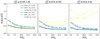 |
Fig. C.1 Accuracy in recovering the Lyα wavelength, thus the redshift, of mock sources using IGM+z (blue), IGM-z (green) and NoIGM (yellow). From left to right subsamples with intrinsic |

 |
Fig. C.2 Accuracy measured through the standard deviation of the difference between the true output parameters and those predicted by IGM+z. The top row shows the accuracy in rest frame wavelength of Lyα, the outflow expansion velocity and the outflow neutral hydrogen column density from left to right. In the bottom row we show the accuracy for the intrinsic equivalent width and width before entering into the ISM and |


Appendix D Examples of line profile reconstruction
In this section we show several examples of the performance of zELDA in reconstructing the shape of mock Lyα line profiles. In Fig. D.1 we show 20 individual cases from from z = 0 up to z = 6.0 in which the reconstruction is successful in the IGM+z and IGM-z models. Then, in Fig. D.2 we show 8 examples in which the Lyα line is not reconstructed properly. Both, Fig. D.1 and D.2 follow the same structure. In each panel, the intrinsic Lyα line profile leaving the galaxy is shown in red, while the IGM transmission curve is shown in pink. The mock observed Lyα line profiles used to build the input for the ANN models are shown in black. The quality of the mock line profiles is S/Np = 15.0, Wg is 0.1(1 + z) so that the resolution element is constant in rest frame, and ΔλPix = Wg/2. zELDA’s prediction using IGM+z, IGM-z and NoIGM are displayed in blue, green and yellow, respectively. The true  is shown in black, while the predictions of IGM+z, IGM-z are given in top blue and bottom green, respectively, with their 1σ uncertainty. Kolmogorov-Smirnov is shown for IGM+z, IGM-z and NoIGM, from left to right, between the predicted line and the intrinsic (red). The individual cases are discussed in Sect. 4.1.
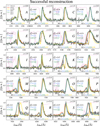 |
Fig. D.1 Examples of line profile successful reconstruction at different redshift. The redshift of the mock line profile is in the top right corner of each subpanel. The Lyα line after the ISM and before traveling through the IGM is shown in red. The IGM transmission curve is shown in pink. The observed line profile, after IGM absorption and mocking observation conditions, is shown in black. S/Np = 15.0 is fixed for all the line profiles. Meanwhile, Wg is 0.1(1+z) so that the resolution element is constant in rest frame. zELDA’s prediction for the models IGM+z, IGM-z and NoIGM are displayed in blue, green and yellow, respectively. In each panel the true |

Appendix E Accuracy in the shape of line profile reconstruction
In this section we study the accuracy in the shape of the recovered intrinsic Lyα line profile. Figure E.1 shows the KS distribution for three mocks made in the same methodology as those for the parameter accuracy (Sect. C). In particular, S/Np = 15.0 and Wg = 0.25 Å, S/Np = 10.0 and Wg = 0.5 Å and S/Np = 7.5 and Wg = 1.0 Å are shown from left to right. The KS distribution of the predicted Lyα line profiles by IGM+z, IGM-z and NoIGM are shown in blue, green and yellow, respectively. The horizontal dashed lines indicate the median of each distribution. In general, we find that IGM+z and IGM-z outperform NoIGM. While there is a significant difference between the accuracy of IGM+z and IGM-z and NoIGM, IGM-z performs slightly better than IGM+z. IGM+z and IGM-z show a median value around 10−1.5 while the median KS value of NoIGM is around 10−1.2.
In Fig. E.2 we show the evolution as a function of S/Np of the percentile of sources with a better KS than 0.1. In some sense, these curves would show the percentage of sources for with the line profile shape is recovered correctly. For other KS thresholds the curves follow the same trends. Figure E.2 shows three scenarios with different ISM attenuation, being stronger on the right panel. We find that for better spectral quality (solid line) the percentage of line profiles recovered correctly increases, specially with S/Np. While IGM+z and IGM-z behave similarly at  ∼0.6, the NoIGM model decreases severely its efficiency.
In Fig. E.3 we show the median of the KS distribution for the Lyα line profile mocks shown in Sect. C as a function of  and for IGM+z, IGM-z and NoIGM, from left to right. As expected, the Lyα line profile shape are better recover at better spectral quality configurations. As for the outflow parameters, we find that NoIGM outperforms IGM+z and IGM-z in the
  ∈[0.95,1.0] regime. Also, the line profile accuracy of NoIGM drops fast with
  . In the best scenario (Wg = 0.1 and S/Np = 15.0), at
  ∈[0.95,1.0], the median KS is 0.01, at
  ∈ [0.8, 0.95] is 0.04 and at
  ∈ [0.35, 0.5] is 0.13. Meanwhile, IGM+Z and IGM-Z Lyα line profile reconstruction is better than that of NoIGM for
  < 0.95. In particular, for IGM+z and IGM-z the median KS is generally below 0.05 in all the quality configurations explored. Although for Wg = 4.0 Å and small
  values, the median KS goes up to 0.9.
In Sect. 4 we show that in some cases and outflow configuration after passing through the IGM might resembles another outflow configuration. This causes confusion when reconstructing the Lyα lines (see examples in Fig. D.2). In order to quantify the fraction of cases in which our ANN models reconstruct properly the Lyα we show in Fig. E.4 the percentile at which KS=0.1. In general, reconstructed Lyα line profiles with KS=0.1 are correctly recovered. Although in some cases Lyα lines with KS >0.1 are properly recovered (and vice verse), the KS=0.1 threshold is in general valid. We find the same general trends for smaller KS thresholds like 0.08.
As expected, the percentile at which KS=0.1(Q(KS = 0.1)) depends on the Lyα line profile quality. The better the spectral quality, the higher the Q(KS = 0.1) is. As before, NoIGM outperforms IGM+z and IGM-z in the unabsorbed regime, being Q(KS = 0.1) = 98%, 0.96% and 0.96% respectively at the best configuration. However, IGM+z and IGM-z outperform NoIGM when  < 0.95. Remarkably Q(KS = 0.1) is greater than the 90% for many quality configurations. Also, we find that for S/Np > 7.5 and
  >0.5 the Q(KS = 0.1)>70% typically, even at Wg = 4.0 Å.
Notice that the outflow model confusion described in Sect. C is not the only contributor to Q(KS = 0.1). The information destroyed by pixelization and noise affect Q(KS = 0.1). For instance, Q(KS = 0.1) for NoIGM, in the unabsorbed regime, goes from 98% in the best quality scenario down to 67% at the worst spectral quality.
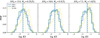 |
Fig. E.1 Kolmogórov-Smirnov estimator distribution comparison between models. zELDA’s prediction using the IGM+z, IGM-z and NoIGM models are displayed in blue, green and yellow, respectively. Each subpanel show the KS distribution at different observed line profile qualities. In particular, in the left panel S/Np = 15.0 and Wg = 0.25 Å, in the middle panel S/Np = 10.0 and Wg = 0.5 Å, in the right panel S/Np = 7.0 and Wg = 1.0 Å. The vertical dashed lines mark the median of the KS distribution of the matching color. |
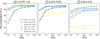 |
Fig. E.2 Percentile of sources with Kolmogórov-Smirnov estimator better than 0.1 at different spectral qualities (the dashed line uses a Wg = 1.0 Å and the solid line Wg = 0.25 Å.) for the three models (IGM+z (blue), IGM-z (green) and NoIGM (yellow)) and for three |

 |
Fig. E.3 Median of the Kolmogórov-Smirnov distribution comparison between observed line profiles quality configurations and zELDA’s models. The IGM+z, IGM-z and NoIGM are shown from left to right. Lighter colors match smaller number and vice versa. |
 |
Fig. E.4 Percentile in the Kolmogórov-Smirnov distribution at which KS=0.1 for IGM+z, IGM-z and NoIGM are shown from left to right. Lighter colors match smaller number and vice versa. |
Appendix F Alternative models for  inference
In this section we explore zELDA’s capability to reconstruct the stack (or average) of intrinsic Lyα line profiles when the intrinsic spectrum does not evolve with redshift. In this example, Mock_fix, all line profiles are configured with identical outflow parameters: Vexp = 200.0 km s−1, NH = 19.3 cm−2, EWin 20.0 Å, Win 2.0 Å, and τa = 0.001. These parameters were selected to ensure that the intrinsic line profile matched the observed stack of Lyα line profiles at low redshift (Hayes et al. 2023). The results for this analysis are shown in Fig. F.1 and discussed in Sect..
Appendix G Alternative models for  inference
In this section we briefly discuss another model, REC+z. REC+z uses the recalibrated IGM transmission curves (as IGM-z) at the source redshift includes it in the input (as IGM+z). The redshift evolution in the  distribution in shown in the left panel of Fig. G.1. The REC+z model shows a similar
  distribution as IGM+z (see Fig. 5), however, at z < 1.0 the dispersion in REC+z is smaller, as 2σ of the sources have
  > 0.9. In comparison, in IGM+z more than 2σ of the sources exhibit
  > 0.8 at z < 1.0. The small variance at z < 1.0 in this training set is due to the fact that the IGM absorption at the Lyα wavelength is suppressed after the recalibration (see the right panel of Fig. 2).
The small scatter causes that REC+z  measurements are biased towards high values at z < 1.0. This is shown in the right panel of Fig. G.1. Focusing in the mock 4 (grey), REC+z predicts a
  about 0.9 when the true
  is 0.8 at z < 1.0. Similarly, this is also clear in mock 3 (blue). The over prediction in REC+z at z < 1.0 is caused by the small
  scatter of the training set. As in the training set there is no source with
  ∼ 0.8 at z < 1.0, REC+z does not predicts
  ∼ 0.8 values at z < 1.0 even if the source true
  is 0.8.
In the development of this work we have tested several alternative models, such as REC+z. We found that IGM+z and IGM-z were the most unbiased models among those explored. In particular, a few models, just as REC+z, were biased in the low redshift regime while they performed correctly at high redshift. For these reason, we display mainly IGM+z and IGM-z in this work. Meanwhile, in the zELDA package, in addition to IGM+z and IGM-z, the other tested models are also included.
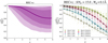 |
Fig. G.1 Left: |

References
- Ahn, S., 2003, J. Korean Astron. Soc., 36, 145 [Google Scholar]
- Behrens, C., Pallottini, A., Ferrara, A., Gallerani, S., & Vallini, L., 2019, MNRAS, 486, 2197 [NASA ADS] [CrossRef] [Google Scholar]
- Byrohl, C., & Gronke, M., 2020, A&A, 642, L16 [NASA ADS] [CrossRef] [EDP Sciences] [Google Scholar]
- Byrohl, C., Saito, S., & Behrens, C., 2019, MNRAS, 489, 3472 [Google Scholar]
- Byrohl, C., Nelson, D., Behrens, C., et al. 2021, MNRAS, 506, 5129 [NASA ADS] [CrossRef] [Google Scholar]
- Caruana, J., Wisotzki, L., Herenz, E. C., et al. 2020, VizieR Online Data Catalog: J/MNRAS/473/30 [Google Scholar]
- Dijkstra, M., Haiman, Z., & Spaans, M., 2006, ApJ, 649, 14 [NASA ADS] [CrossRef] [Google Scholar]
- Farrow, D. J., Sánchez, A. G., Ciardullo, R., et al. 2021, MNRAS, 507, 3187 [Google Scholar]
- Faucher-Giguère, C.-A., Prochaska, J. X., Lidz, A., Hernquist, L., & Zaldarriaga, M., 2008, ApJ, 681, 831 [Google Scholar]
- Green, J. C., Froning, C. S., Osterman, S., et al. 2012, ApJ, 744, 60 [NASA ADS] [CrossRef] [Google Scholar]
- Greene, J., Bezanson, R., Ouchi, M., Silverman, J., & the PFS Galaxy Evolution Working Group. 2022, arXiv e-prints [arXiv:2206.14908] [Google Scholar]
- Gronke, M., 2017, A&A, 608, A139 [NASA ADS] [CrossRef] [EDP Sciences] [Google Scholar]
- Gronke, M., Dijkstra, M., McCourt, M., & Oh, S. P., 2016, ApJ, 833, L26 [CrossRef] [Google Scholar]
- Gurung-López, S., Orsi, Á. A., & Bonoli, S. 2019a, MNRAS, 490, 733 [CrossRef] [Google Scholar]
- Gurung-López, S., Orsi, Á. A., Bonoli, S., Baugh, C. M., & Lacey, C. G. 2019b, MNRAS, 486, 1882 [Google Scholar]
- Gurung-López, S., Orsi, Á. A., Bonoli, S., et al. 2020, MNRAS, 491, 3266 [Google Scholar]
- Gurung-López, S., Saito, S., Baugh, C. M., et al. 2021, MNRAS, 500, 603 [Google Scholar]
- Gurung-López, S., Gronke, M., Saito, S., Bonoli, S., & Orsi, Á. A. 2022, MNRAS, 510, 4525 [NASA ADS] [CrossRef] [Google Scholar]
- Harris, C. R., Millman, K. J., van der Walt, S. J., et al. 2020, Nature, 585, 357 [NASA ADS] [CrossRef] [Google Scholar]
- Hayes, M. J., Runnholm, A., Scarlata, C., Gronke, M., & Rivera-Thorsen, T. E., 2023, MNRAS, 520, 5903 [NASA ADS] [CrossRef] [Google Scholar]
- Herenz, E. C., Urrutia, T., Wisotzki, L., et al. 2017, A&A, 606, A12 [NASA ADS] [CrossRef] [EDP Sciences] [Google Scholar]
- Hill, G. J., Gebhardt, K., Komatsu, E., et al. 2008, in Astronomical Society of the Pacific Conference Series, 399, Astronomical Society of the Pacific Conference Series, eds. T. Kodama, T. Yamada, & K. Aoki, 115 [Google Scholar]
- Hunter, J. D., 2007, Comput. Sci. Eng., 9, 90 [NASA ADS] [CrossRef] [Google Scholar]
- Kakuma, R., Ouchi, M., Harikane, Y., et al. 2021, ApJ, 916, 22 [NASA ADS] [CrossRef] [Google Scholar]
- Laursen, P., Sommer-Larsen, J., & Razoumov, A. O., 2011, ApJ, 728, 52 [Google Scholar]
- Marinacci, F., Vogelsberger, M., Pakmor, R., et al. 2018, MNRAS, 480, 5113 [NASA ADS] [Google Scholar]
- Mason, C. A., & Gronke, M., 2020, MNRAS, 499, 1395 [Google Scholar]
- Naiman, J. P., Pillepich, A., Springel, V., et al. 2018, MNRAS, 477, 1206 [Google Scholar]
- Nelson, D., Springel, V., Pillepich, A., et al. 2019, Computat. Astrophys. Cosmol., 6, 2 [Google Scholar]
- Neufeld, D. A., 1990, ApJ, 350, 216 [NASA ADS] [CrossRef] [Google Scholar]
- Orsi, A., Lacey, C. G., & Baugh, C. M., 2012, MNRAS, 425, 87 [NASA ADS] [CrossRef] [Google Scholar]
- Orsi, Á., Padilla, N., Groves, B., et al. 2014, MNRAS, 443, 799 [Google Scholar]
- Ouchi, M., Harikane, Y., Shibuya, T., et al. 2018, PASJ, 70, S13 [Google Scholar]
- Ouchi, M., Ono, Y., & Shibuya, T., 2020, ARA&A, 58, 617 [Google Scholar]
- Pillepich, A., Nelson, D., Hernquist, L., et al. 2018, MNRAS, 475, 648 [Google Scholar]
- Rudie, G. C., Steidel, C. C., & Pettini, M., 2012, ApJ, 757, L30 [Google Scholar]
- Runnholm, A., Gronke, M., & Hayes, M., 2021, PASP, 133, 034507 [CrossRef] [Google Scholar]
- Saxena, A., Bunker, A. J., Jones, G. C., et al. 2024, A&A, 684, A84 [NASA ADS] [CrossRef] [EDP Sciences] [Google Scholar]
- Schaerer, D., Hayes, M., Verhamme, A., & Teyssier, R., 2011, A&A, 531, A12 [NASA ADS] [CrossRef] [EDP Sciences] [Google Scholar]
- Spinoso, D., Orsi, A., López-Sanjuan, C., et al. 2020, A&A, 643, A149 [EDP Sciences] [Google Scholar]
- Springel, V., Pakmor, R., Pillepich, A., et al. 2018, MNRAS, 475, 676 [Google Scholar]
- Steidel, C. C., Erb, D. K., Shapley, A. E., et al. 2010, ApJ, 717, 289 [Google Scholar]
- Torralba-Torregrosa, A., Gurung-López, S., Arnalte-Mur, P., et al. 2023, A&A, 680, A14 [NASA ADS] [CrossRef] [EDP Sciences] [Google Scholar]
- Torralba-Torregrosa, A., Renard, P., Spinoso, D., et al. 2024, A&A, 690, A388 [NASA ADS] [CrossRef] [EDP Sciences] [Google Scholar]
- Urrutia, T., Wisotzki, L., Kerutt, J., et al. 2019, A&A, 624, A141 [NASA ADS] [CrossRef] [EDP Sciences] [Google Scholar]
- Verhamme, A., Schaerer, D., Atek, H., & Tapken, C., 2007, in Astronomical Society of the Pacific Conference Series, 380, Deepest Astronomical Surveys, eds. J. Afonso, H. C. Ferguson, B. Mobasher, & R. Norris, 97 [Google Scholar]
- Verhamme, A., Garel, T., Ventou, E., et al. 2018, MNRAS, 478, L60 [Google Scholar]
- Virtanen, P., Gommers, R., Oliphant, T. E., et al. 2020, Nat. Methods, 17, 261 [Google Scholar]
- Weiss, L. H., Bowman, W. P., Ciardullo, R., et al. 2021, ApJ, 912, 100 [Google Scholar]
- Zheng, Z., Cen, R., Trac, H., & Miralda-Escudé, J., 2011, ApJ, 726, 38 [NASA ADS] [CrossRef] [Google Scholar]
All Tables
Outflow parameters in redshift nodes used for the Lyα-line-profile stacked mocks.
All Figures
|
Fig. 1 Illustration of impact of different lines of sight in the same intrinsic spectrum. In the middle bottom panel, we show the intrinsic spectrum escaping the source (black) convolved with the mean IGM transmission at z = 3.0 (yellow). The colour line shows the convolution of the intrinsic spectrum and IGM transmission. The coloured circles show the zELDA reconstruction using the IGM-z model (discussed later). In the other five top panels, individual IGM transmission through different lines of sight are used at z = 3.0. |
| In the text | |
|
Fig. 2 Mean IGM transmission curves without re-calibration (left) and after re-calibration (right). Each colour shows a different redshift snapshot. The horizontal dashed black lines show the mean IGM transmission given by Faucher-Giguère et al. (2008) at z = 0,1,2,3,4,5 from top to bottom. |
| In the text | |
|
Fig. 3 Example of line-profile reconstruction at different line-profile qualities and using our different models. The true Lyα line before passing through the IGM is displayed in red. The IGM transmission curve is shown in pink. The true Lyα line profile is fixed in each row. The observed line profile, after IGM absorption and mocking observation conditions, is shown in black. The observation conditions are fixed in each column as Wg = 0.25 Å, S/Np = 15.0, Wg = 0.5 Å, S/Np = 10.0, Wg = 1.0 Å, S/Np = 7.0, and Wg = 2.0 Å, S/Np = 5.0 from left to right, respectively. The zELDA prediction for the models IGM+z, IGM-z, and NoIGM are displayed in blue, green, and yellow, respectively. In the bottom of each panel the KS estimation between the true Lyα line profile before the IGM absorption and zELDA prediction is displayed in colours matching the model used. |
| In the text | |
|
Fig. 4 Left: total variance recovered as function of number of principle components. We show Lyα line profiles spamming zELDA’s grid without (with) IGM absorption in red (green). The dashed black line marks the number of principal components used for the input of the artificial neural networks. We fixed the number of PCA to 100 to achieve a re-coverage of 95% of the total variance. Right: example of PCA decomposition in an IGM clean-shell model line profile. The line profiles are shown in the proxy rest frame. The original mock line profile is shown in grey. Meanwhile, the reconstructed line profiles using the N first principal components are displayed in the legend. |
| In the text | |
|
Fig. 5
|
| In the text | |
|
Fig. 6 zELDA’s prediction of mean |
| In the text | |
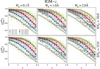 |
Fig. 7 Same as Fig. 6, but for the IGM-z model. |
| In the text | |
|
Fig. 8 Stacked line-profile reconstruction example in mock Lyα line profiles using the Lyα line profiles with redshift dependence. The stacked line profile is shown the redshift intervals [0.75,1.25] (grey), [1.75,2.25] (blue), [2.75,3.25] (green), [3.75,4.25] (yellow), and [4.75,5.25] (red). The Lyα stacked line profiles using the Lyα line profiles before applying the IGM absorption are displayed in the top left panel. The two top right panels display the Lyα stacked line profile after applying the IGM absorption and mocking observation qualities similar to those of HST (Wg=0.1 Å and S/Np = 15.0, top) and MUSE (Wg = 2.0 Å and S/Np = 10.0, bottom). The six bottom panels show the reconstructed stacked Lyα line profiles. Each bottom column makes use of a different ANN model: IGM+z, IGM-z, and NoIGM from left to right. The KS between the stacked Lyα line profile before the IGM (left column) and that of the reconstructed Lyα line profiles is displayed in coloured text matching the redshift bin. |
| In the text | |
|
Fig. A.1 Feature importance analysis for the IGM+z (blue), IGM-z (green) and NoIGM (yellow). For comparison, the stacked line profiles with its 1σ scatter is shown in grey. Each subplot shows the importance determining a different property. In top row, ΔλTrue, EWin, Win from left to right. In the bottom row, NH, Vexp, |
| In the text | |
|
Fig. B.1 Top: Comparison between the fraction of cases that a measurement is in agreement with the intrinsic true value, fcomp, as a function of the confidence level. Bottom: Applied correction factor to uncertainty. The uncorrected fcomp is shown in colored solid lines, which IGM+z in green, IGM-z in blue and NoIGM in yellow. fcomp after the correction is shown in colored dots. In each panel a different output property is shown. In the first row zmax, Vexp and NH from left to right. In the second row τa, EWin, Win, from left to right. In the third row |
| In the text | |
|
Fig. C.1 Accuracy in recovering the Lyα wavelength, thus the redshift, of mock sources using IGM+z (blue), IGM-z (green) and NoIGM (yellow). From left to right subsamples with intrinsic |
| In the text | |
|
Fig. C.2 Accuracy measured through the standard deviation of the difference between the true output parameters and those predicted by IGM+z. The top row shows the accuracy in rest frame wavelength of Lyα, the outflow expansion velocity and the outflow neutral hydrogen column density from left to right. In the bottom row we show the accuracy for the intrinsic equivalent width and width before entering into the ISM and |
| In the text | |
 |
Fig. C.3 Same as Fig. C.2 but for IGM-z. |
| In the text | |
 |
Fig. C.4 Same as Fig. C.2 but for NoIGM. |
| In the text | |
|
Fig. D.1 Examples of line profile successful reconstruction at different redshift. The redshift of the mock line profile is in the top right corner of each subpanel. The Lyα line after the ISM and before traveling through the IGM is shown in red. The IGM transmission curve is shown in pink. The observed line profile, after IGM absorption and mocking observation conditions, is shown in black. S/Np = 15.0 is fixed for all the line profiles. Meanwhile, Wg is 0.1(1+z) so that the resolution element is constant in rest frame. zELDA’s prediction for the models IGM+z, IGM-z and NoIGM are displayed in blue, green and yellow, respectively. In each panel the true |
| In the text | |
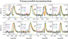 |
Fig. D.2 Same as Fig. D.1 but for unsuccessful reconstructions. |
| In the text | |
|
Fig. E.1 Kolmogórov-Smirnov estimator distribution comparison between models. zELDA’s prediction using the IGM+z, IGM-z and NoIGM models are displayed in blue, green and yellow, respectively. Each subpanel show the KS distribution at different observed line profile qualities. In particular, in the left panel S/Np = 15.0 and Wg = 0.25 Å, in the middle panel S/Np = 10.0 and Wg = 0.5 Å, in the right panel S/Np = 7.0 and Wg = 1.0 Å. The vertical dashed lines mark the median of the KS distribution of the matching color. |
| In the text | |
|
Fig. E.2 Percentile of sources with Kolmogórov-Smirnov estimator better than 0.1 at different spectral qualities (the dashed line uses a Wg = 1.0 Å and the solid line Wg = 0.25 Å.) for the three models (IGM+z (blue), IGM-z (green) and NoIGM (yellow)) and for three |
| In the text | |
|
Fig. E.3 Median of the Kolmogórov-Smirnov distribution comparison between observed line profiles quality configurations and zELDA’s models. The IGM+z, IGM-z and NoIGM are shown from left to right. Lighter colors match smaller number and vice versa. |
| In the text | |
|
Fig. E.4 Percentile in the Kolmogórov-Smirnov distribution at which KS=0.1 for IGM+z, IGM-z and NoIGM are shown from left to right. Lighter colors match smaller number and vice versa. |
| In the text | |
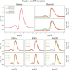 |
Fig. F.1 Same as Fig. 8 but for the redshift invariant Lyα line profiles. |
| In the text | |
|
Fig. G.1 Left: |
| In the text | |
Current usage metrics show cumulative count of Article Views (full-text article views including HTML views, PDF and ePub downloads, according to the available data) and Abstracts Views on Vision4Press platform.
Data correspond to usage on the plateform after 2015. The current usage metrics is available 48-96 hours after online publication and is updated daily on week days.
Initial download of the metrics may take a while.