| Issue |
A&A
Volume 642, October 2020
|
|
|---|---|---|
| Article Number | L16 | |
| Number of page(s) | 8 | |
| Section | Letters to the Editor | |
| DOI | https://doi.org/10.1051/0004-6361/202038685 | |
| Published online | 19 October 2020 | |
Letter to the Editor
Variations in shape among observed Lyman-α spectra due to intergalactic absorption
1
Max-Planck-Institut für Astrophysik, Karl-Schwarzschild-Str. 1, 85748 Garching, Germany
e-mail: This email address is being protected from spambots. You need JavaScript enabled to view it.
2
Department of Physics and Astronomy, Johns Hopkins University, Baltimore, MD 21218, USA
3
Department of Physics and Astronomy, University of California, Santa Barbara, CA 93106, USA
Received:
18
June
2020
Accepted:
4
September
2020
Abstract
Lyman-α (Lyα) spectra provide insights into the small-scale structure and kinematics of neutral hydrogen (HI) within galaxies as well as the ionization state of the intergalactic medium (IGM). The former defines the intrinsic spectrum of a galaxy, which, in turn, is modified by the latter. These two effects are degenerate. Using the IllustrisTNG100 simulation, we studied the impact of the IGM on Lyα spectral shapes between z ∼ 0 and 5. We computed the distribution of the expected Lyα peaks and of the peak asymmetry for different intrinsic spectra, redshifts, and large-scale environments. We find that the averaged transmission curves that are commonly applied give a misleading perception of the observed spectral properties. We show that the distributions of peak counts and asymmetry can lift the degeneracy between the intrinsic spectrum and IGM absorption. For example, we expect a significant number of triple-peaked Lyα spectra (up to 30% at z ∼ 3) if the galaxies’ HI distribution become more porous at higher redshift, as predicted by cosmological simulations. We provide a public catalog of transmission curves for simulations and observations to allow for a more realistic IGM treatment in future studies.
Key words: radiative transfer / intergalactic medium / large-scale structure of Universe / galaxies: high-redshift
Hubble fellow.
© C. Byrohl and M. Gronke 2020
 Open Access article, published by EDP Sciences, under the terms of the Creative Commons Attribution License (https://creativecommons.org/licenses/by/4.0), which permits unrestricted use, distribution, and reproduction in any medium, provided the original work is properly cited.
Open Access funding provided by Max Planck Society.
1. Introduction
The Lyman-α (Lyα) line is a promising astrophysical observable for the neutral hydrogen distribution, from the scale of parsecs in star-forming regions (e.g., Kunth et al. 1998; Yang et al. 2016) all the way to cosmological scales. As such, it is among the most powerful observables to constrain the cosmic neutral fraction during the Epoch of Reionization (e.g., Dijkstra 2014; Mason et al. 2019).
While Lyα observations allow us to tackle a wide range of astrophysical questions, probing different spatial scales is a challenge because of a possible degeneracy of the origin of spectral features in those observations. Lyα observables are shaped not only through the neutral hydrogen (HI) distribution and the kinematics internal to galaxies, that is, the interstellar medium (ISM), but also by HI residing in the circumgalactic medium (CGM; Steidel et al. 2011; Wisotzki et al. 2016) and the intergalactic medium (IGM).
At low redshift (z ≲ 1), the impact of the IGM is very limited due to low neutral hydrogen fractions, such that observations with the Hubble Space Telescope reveal the spectral features imprinted by the ISM and CGM only. Usually, Lyα spectra show very little flux at line-center (λc ∼ 1216 Å), and emission mostly originates on the red (λ > λc) side of the spectrum, with a significant fraction of spectra showing essentially no flux on the blue (λ < λc) side (Östlin et al. 2014; Hayes et al. 2014; Henry et al. 2015; Yang et al. 2016; review by Hayes 2015).
At higher redshifts, however, the impact of the IGM increases and the picture is less certain. Individual observations at z ∼ 5 − 7 mainly show a single peak redshifted by a few hundred km s−1 (Matthee et al. 2017). At intermediate redshifts, larger statistical samples do measure an asymmetry toward the red (Erb et al. 2014). This spectral evolution leaves, in principle, two possibilities: either the “intrinsic” Lyα spectra emergent from the galaxies do not vary strongly with redshift or they vary, but the IGM transmission, which is also evolving, makes the observed spectral properties remain similar. While the former scenario is supported by the fact that the low-z samples are selected as “analogs” of higher redshift Lyα emitters (e.g., Yang et al. 2016), the latter is suggested by modern radiative transfer simulations using galactic hydrodynamical simulations as input (e.g., Laursen et al. 2011; Gronke et al. 2018; Smith et al. 2019). Due to strong feedback mechanisms, they produce a porous ISM at high-z, and thus, the predicted Lyα spectra exhibit relatively large flux at line-center and the blue side of the spectrum. Differentiating between these pathways is crucial to properly disentangle the Lyα line’s use as a probe of galaxy and IGM evolution.
While recent studies have focused mainly on the intragalactic Lyα transfer (e.g., Smith et al. 2019), less attention has been devoted to the effect of the IGM on the Lyα spectral shape. Even large-scale studies that include the IGM have focused primarily on global statistics, such as the Lyα emitter clustering or luminosity function (e.g., Iliev et al. 2008; Zheng et al. 2010; Behrens et al. 2018; Byrohl et al. 2019). In this paper, we seek to clarify the IGM’s impact on the Lyα spectra using using a recent cosmological simulation in the redshift range of z = 0 − 5.
2. Methodology
2.1. Simulations
We analyzed the IGM attenuation using the IllustrisTNG100 simulations (Naiman et al. 2018; Nelson et al. 2018; Marinacci et al. 2018; Pillepich et al. 2018; Springel et al. 2018) with a box size of 106.5 comoving Mpc for redshifts 0.0, 1.0, 2.0, 3.0, 4.0, and 5.0. The attenuation of Lyα flux was calculated with a modified version of ILTIS1, a line emission transfer code as per Behrens et al. (2019), which traces the optical depth in the IGM between the Lyα emitting galaxies and the observer for chosen lines of sight. The code was modified to natively run on IllustrisTNG’s Voronoi tessellation. The initial tessellation was created with a parallelized wrapper of voro++ (Rycroft 2009) on IllustrisTNG’s particle distribution. IllustrisTNG uses a time variable UV background with self-shielding (Faucher-Giguère et al. 2009; Rahmati et al. 2013) as well as a mimicking of the effect of active galactic nuclei (AGN) on the local radiation field (Vogelsberger et al. 2013) that is responsible for the hydrogen’s ionization state in the IGM. Due to the long mean-free path of ionizing photons at the considered redshifts (z ≤ 5) and our exclusion of HI close to star-forming regions (see below), using a full radiation hydrodynamics simulation as input would not change the outcome of our study.
The optical depth, τ, is integrated over the intervening medium for given lines of sight and a given input wavelength, λi. The optical depth along the way can be expressed by
 (1)
(1)
where nHI is the neutral hydrogen density and σ(λ) is the Lyα cross-section. In Eq. (1), we integrate over the physical distance, s, from the source along the chosen lines of sight (LOS). The temperature, THI, sets the thermal broadening reshaping the cross-section profile σ. The cross-section is evaluated in the rest-frame of the gas and, thus, depends on the peculiar velocity v and Hubble flow H(z) at redshift z. The wavelength is shifted as ![Mathematical equation: $ \lambda = \lambda_{\mathrm{i}}\left[1+\frac{v(s)+H(z)\cdot s}{c}\right] $](/articles/aa/full_html/2020/10/aa38685-20/aa38685-20-eq2.gif) , where c is the speed of light. We commonly express the wavelength as its offset Δλe = λ − λc from the Lyα line-center at the emitters’ redshift.
, where c is the speed of light. We commonly express the wavelength as its offset Δλe = λ − λc from the Lyα line-center at the emitters’ redshift.
The input wavelengths λi are evaluated in the rest-frame of the halos, which we identify as the mass-weighted velocity. We compute the optical depth within the wavelength range [λc − 5 Å, λc + 3 Å] with a resolution of 0.02 Å (R ∼ 60 000). For the IGM attenuation, we start summing contributions to the optical depth from a distance s0 = frvir, where rvir the virial radius of the halo. For a comparison with Laursen et al. (2011), we chose f = 1.5. This implies that while photons are redshifted by the Hubble flow, no contributions to the optical depth are considered for r < s0. The robustness of the chosen s0 is confirmed in Appendix B. We integrate to 30 cMpc h−1 using periodic boundary conditions for the box. This length corresponds to a Hubble shift of 2600 km s−1 (at z = 1.0) or more. We verified that for the chosen input wavelength range λi, all wavelengths have significantly redshifted beyond the Lyα line-center as facilitated by the Hubble flow and, thus, no attenuation contributions are expected beyond this upper integration limit.
In our analysis, we consider the centers of halos as possible Lyα-emitting galaxies if they contain regions of active star formation and have a total halo mass above 5 ⋅ 109 M⊙, as provided by IllustrisTNG’s friends-of-friends halo catalogs. For each emitter, we evaluate the optical depth along 1000 LOS. The LOS are constructed as normal vectors of a 1000-faced Fibonacci sphere, evenly tracing possible directions with the same normal vectors used throughout. A reduced public data set of our transmission curves has been published as Byrohl & Gronke (2020) and a full data set can be made available upon request.
2.2. Input spectra
To demonstrate how the IGM attenuation affects the observed spectra in a statistical sample using the individual attenuation curves, we need to assume some input (intrinsic) spectra with flux density Iλ, input. Here, we use three different toy models:
First, we have a symmetric double peaked profile as result of a static neutral hydrogen sphere, also referred to as Neufeld solution (Neufeld 1990; Dijkstra et al. 2006). We set the temperature as THI = 104 K and the column density to NHI = 1020 cm−2 for this model.
Second, we consider red peak only that corresponds to the Neufeld solution under the assumption of a significant outflow. These two spectral shapes bracket the observed cases at low-z, which largely consist of a single or double peak dominant toward the red.
Third, we assume a Gaussian at Lyα line-center with a width of σ = 200 km s−1 as input spectrum. Such a setup with a significant line-center flux can be motivated for galaxies with a larger impact of stellar feedback at high redshifts leaving a more porous HI distribution. Lyα photons then escape closer to the line-center and are less susceptible to the gas kinematics (Neufeld 1991; Hansen & Oh 2006; Gronke & Dijkstra 2016). For this reason, recent galactic hydrodynamical models post-processed with Lyα radiative transfer show a wide, fairly symmetric intrinsic profile with little absorption at line-center emergent from these galaxies (e.g., Smith et al. 2019). The width was chosen to approximately match the predictions of those models.
3. Results
3.1. Averaged transmission curves
In Fig. 1, we show the resulting spectrum along three LOS for the same origin with the Gaussian and double-peaked input spectra. In this plot, and in general, it is mostly the spectrum blueward of the line-center that is affected as those frequencies will eventually shift into the line-center by the Hubble flow. Figure 1 shows that the transmission blueward of the line-center can fluctuate strongly for different wavelengths of a given line of sight. In fact, the LOS in Fig. 1 have been chosen such that the blue side of the observed spectrum exhibits a varying count of spectral peaks between zero and two for the Neufeld input spectrum. We formalize the count of peaks into a quantitative measure in Sect. 3.2.1. The transmission function is given as
![Mathematical equation: $$ \begin{aligned} T(\Delta \lambda _e) = \exp \left[-\tau (\Delta \lambda _e)\right] \end{aligned} $$](/articles/aa/full_html/2020/10/aa38685-20/aa38685-20-eq3.gif) (2)
(2)
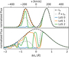 |
Fig. 1. Panels showing two different input (i.e., intrinsic) spectra (black lines) and how the IGM attenuation shapes the observed spectra along different LOS at z = 3.0. All spectra are normalized by the respective underlying input spectrum’s total flux. The gray dashed line shows the multiplication of the respective input spectrum with the median transmission curve, |

and describes the fraction of the overall flux attenuated by the IGM between the emitter and the observer.
In Fig. 2, we show the probability density function (PDF) p(T, Δλe) of the transmission function T averaged over all emitters and LOS at z = 3. We also plot the mean and median curves (blue/green bold lines) along with the central 68 percentiles (hatched area). From these curves, it is clear that the blue side is suppressed by roughly a factor of two, while the red side is mostly unaffected. We find a trough around line-center suppressing most of the flux. In general, we find these curves to be consistent with the results found by Laursen et al. (2011) and Gurung-López et al. (2020). Discrepancies in the asymptotic median value and the shaded 16th–84th percentile region are mostly a result of these quantities being highly dependent on the spectral resolution (see Appendix A). The spectral resolution in the literature is significantly lower with R ≲ 3000 than R ∼ 60 000 used here.
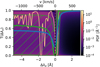 |
Fig. 2. PDF of the transmission, T, as a function input wavelength shift, Δλe, over all emitters and the LOS at z = 3. Green line shows the median transmission with the hatched region enclosing the central 68% of all individual transmission curves, while the blue line shows the mean transmission curve over this PDF. The light orange curve shows an example of an individual LOS (corresponding to “LOS 1” in Fig. 1). |
For other redshifts, we find a similar qualitative trend over the shown wavelength range: the transmission on the blue side is increasingly suppressed at higher redshifts with a smaller asymptotic value toward Δλe = −5 Å and a deeper trough around Δλe = 0 Å. We find the most likely offset for this central trough to be roughly 20 km s−1 at z = 0.0, monotonically increasing toward 70 km s−1 at z = 5.0. These velocity offsets and their redshift evolution are consistent with expected halo infall velocities at r = 1.5rvir (Barkana 2004).
As illustrated by Figs. 1 and 2, overall, the median curve is misleading and should be interpreted with caution: the underlying PDF p(T|Δλe) of transmission T(Δλe) is usually bimodal, that is, due to the large Lyα cross-section, it is mostly close to zero or unity – which is not well-represented by averaged transmission curves. For instance, in Fig. 2, the bimodal distribution peaks around 0.0/0.9 (0.0/1.0) on the blue (red) side at z = 3.0. These features can be seen more clearly in Appendix C.
While this bimodality becomes more pronounced at lower redshifts, a unimodal distribution with ⟨T(Δλe)⟩ ∼ 0 forms at higher redshifts as the upper bimodal transmission peak disappears. This bimodal behavior has significant consequences for the observed spectra. Rather than blue peaks being uniformly suppressed along different LOS, some LOS will show a strong blue feature while others will show none. Similarly there also is some variation for red peaks close to the line-center being suppressed given the bimodality there. In Sect. 3.2, we investigate two different quantitative measures to characterize the spectral variations for different lines of sight as implied here.
3.2. Variations in transmission curves
After studying the averaged transmission curves, we proceed to quantify the variations of the transmission curves. Those variations are observable features of the emerging spectra after traversing the IGM.
3.2.1. Peak distribution
As discussed in Sects. 1 and 2.2, the observed Lyα spectra at a low z usually exhibit a double or single red peaked spectrum. Attenuation in the IGM can modify the observed peak count in some LOS.
For an observed spectral flux density Iλ(Δλ), we define a peak as connected flux density bins such that Iλ(Δλ) > IT for a threshold IT. Here, we set IT = 0.01 ⋅ max0 < λ < ∞(Iλ, input). This criterion (while not its specific value) seeks to represent the flux sensitivity of a generic instrument. Furthermore, we require distinct connected areas to have a minimal separation of 0.2 Å (R ∼ 6000) from one another. This criterion is aimed at avoiding any false identification of multiple peaks due to very small flux discontinuities that might additionally be below the spectral resolution of the spectrograph.
Figure 3 shows the distribution of the spectral peak count 0 ≤ Npeaks ≤ 3 over the redshift range from 0 to 5 for the different input spectra. Hardly any LOS exist with Npeaks > 3. The evolution with redshift is anchored by the intrinsic value of Npeaks at z ∼ 0 (i.e., Npeaks = 2 and 1 for the double peaked input spectrum and the other two, respectively) and a single red peak at z = 5, while in roughly 7% of all LOS, nearly all flux, and thus all peaks, are suppressed at z = 5. For the intermediate redshifts, the rugged transmission curve (cf. Sect. 3.1) causes small attenuation features that substantially increase the number of observable peaks for the wide, central input spectrum. Specifically, the number of resultant double and even triple peaks increases to ∼50% and 30% at z ∼ 2 − 4, respectively. Given that at higher redshifts, attenuation features become wider and only the most redward peak survives, this gives a typical U-shaped evolution for Npeaks 1 to 3 in this case. For the same reason, there is a slight U-shape in the triple peak count of the double peaked input spectrum. As the triple peak count is significantly at intermediate redshift, such a count is crucial in differentiating possible scenarios for the small-scale input spectra.
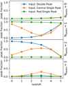 |
Fig. 3. Evolution of detectable Lyα peaks assuming the three different intrinsic spectra as described in Sect. 2.2. The peak detection algorithm is described in Sect. 3.2.1. |
3.2.2. Blue peak flux
We introduce two observables to quantify the peak asymmetry. Namely, the flux ratio Lratio between the integrated flux Lblue for wavelengths below the line-center and the total observed flux (Lblue + Lred):
 (3)
(3)
Analogously, we define the peak flux ratio Fratio as the ratio of maximal flux blueward to the sum of the peak fluxes on both sides of the line-center, namely:
 (4)
(4)
We note that observational studies have used similar measures in the past (e.g., Erb et al. 2014; Verhamme et al. 2017).
In Fig. 4, we show the distributions of Lratio and Fratio across all LOS (with both directions and emitters) using the double peaked intrinsic spectrum introduced in Sect. 2.2. The distribution looks very similar when using the Gaussian input spectrum. We note that, in addition, we imposed a minimum flux on each side of the line-center of 1% the flux of the input spectrum for a LOS to be deemed detectable. A ratio of 0.5 signifies an equal impact of the IGM on the blue and red side of the line-center. Thus, while Fig. 4 makes a prediction for the observed distribution given the idealized input spectrum, it also represents the IGM’s impact on the asymmetry as such, indicating a favorable escape of blue (red) photons through the IGM for values over (below) 0.5.
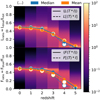 |
Fig. 4. Ratios Lratio (top) and Fratio (bottom) shown as a PDF over all lines of sight for both all directions and emitters at a given redshift as shown by the colormap. We chose the double peaked input spectrum, but we also find a very similar result for the centrally peaked input spectrum. The four overplotted lines in each panel show different averaging methods (see text). We assume that no peak can be detected (hence no ratio) when the flux remaining after passing the IGM is less than 1% of the intrinsic flux I(λ). |
The solid lines show the mean and the median for the ratios, while the dashed lines show ratio for the mean and median transmission curves ⟨T(Δλ)⟩ multiplied by the input spectra. Both ratios intuitively follow the expected redshift evolution for all lines: At redshift z = 0, the asymmetry is mostly unaffected by the IGM, while at higher redshifts the averaged ratios drop toward zero at z = 5 as the IGM becomes more opaque due to a higher HI density. A closer look at the peak asymmetry distribution at a given redshift reveals a more nuanced picture: At low to intermediate redshifts (z ≲ 3), the distribution appears somewhat symmetric around the median with increasing variance and skewness for higher redshifts. Therefore, blue peaks can be prominent features of a fraction of observed spectra even at high redshifts. We find fractions of 13.5%, 17.5%, 14.3%, 8.5%, 4.1%, and 1.8% from redshift 0 to 5, enhancing the blue side of the spectrum (i.e., Lratio > 0.5). Observational studies calculating the enhanced blue peak fraction exist (Erb et al. 2014; Trainor et al. 2015) with up to 16 − 22% at z ∼ 3. However, a fair comparison is not possible due to small number statistics, a varying definition of the flux ratio, and the very low spectral resolution. Future studies overcoming these challenges would be useful for constraining the (a)symmetry of the small-scale spectra.
A range of spectra will continue to contain significant blue contributions at high redshifts. This is another reason why the use of the averaged transmission curves could be misleading with regard to the underlying peak asymmetry distribution. For instance, for z = 5.0, the median transmission curve leads to a Lratio on sub-percent level, leading to the perception that blue peaks are singularities at such redshift, when in reality we find roughly 4% of Lyα emitting galaxies that still show significant blue flux (Lblue ≥ 0.25 ⋅ Lred; analogously, for F, we even find 10%). For the other redshifts (0, 1, 2, 3, and 4) we find 99.5%, 97.0%, 91.8%, 75.5%, and 33.3% of LOS with significant blue flux (if present intrinsically).
3.2.3. Large-scale environment
Beside the redshift and input spectrum, we find that our proposed statistics also depend on the emitters’ large-scale environment. Most prominently, we find a correlation of the flux ratio and peak fraction with the linear overdensity as shown in Fig. 5 for z = 4.0. We calculate the overdensity using a Gaussian smoothing kernel with σ = 3 cMpc h−1. The flux ratio slightly decreases toward higher overdensities indicating more intervening HI. Additionally, the scatter of the flux ratio strongly increases as more varying matter structure is passed along the LOS. The fraction of double peaks, as present in the input spectrum, strongly decreases toward higher overdensities as more blue peaks are attenuated. In up to 10% of the cases, the red peak is additionally suppressed, completely obscuring those Lyα emitting galaxies in high overdensity environments. This also affects the clustering signal of Lyα emitters, as has been studied by Zheng et al. (2011) and Behrens et al. (2018) in more detail. The correlation with overdensity is much weaker for redshift between z = 0.0 and 2.0, where the most likely outcome remains Lratio = 0.5 over the overdensity range. This behavior changes for z = 3.0 and z = 4.0 in overdense regions, where the distribution starts to get skewed toward Lratio close to zero. At higher redshifts, the correlation appears to be smaller as most blue peaks are already attenuated even in underdense regions.
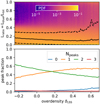 |
Fig. 5. Lratio and Npeaks statistics shown as a function of the large scale overdensity δLSS at redshift z = 4.0. The input spectrum is the Neufeld solution. The colormap in the upper panel shows the underlying PDF normalized at a given δLSS. Overdense regions overall decrease Lratio. At a higher overdensity, this trend halts as the ratio becomes more fluctuating for different LOS. For the peak fractions, we find a gradual decrease of double peaks. This is caused by absorption features on the blue side of the line-center. Thus, the decrease of double peaks is strongly correlated with the increase of the fraction of single peaked spectra. |
4. Conclusions
The Lyα line can be used to constrain the neutral hydrogen distribution from galactic to cosmological scales. This versatility is, however, also a problematic since degeneracies between these scales exist that come into play at z ≳ 3, when the more opaque IGM can compensate the effects of a more porous ISM. Such a scenario – which is suggested by cosmological simulations – allows not only for the escape of Lyα photons closer to line-center but also the escape of ionizing photons that are susceptible to the same galactic HI distribution (e.g., Dijkstra et al. 2016).
Using a large set of transmission curves that we calculated from the IllustrisTNG100 simulations, we quantified the impact of the IGM on spectra for z = 0 − 5. In doing so, we studied a new approach to breaking the degeneracy using two statistics, namely the peak count and peak asymmetry (Sects. 3.2.1/3.2.2). In particular, we found the fraction of triple peaks to be an important differentiator for different intrinsic spectra. In contrast, we show that the commonly used averaged transmission curves can be misleading with regard to the interpretation of the impact of the IGM on observed Lyα spectra and their redshift evolution.
Making our catalogs of transmission curves publicly available (Byrohl & Gronke 2020) opens this work up to other studies that look to incorporate an improved approach to IGM treatment and its impact on Lyα spectra. At the same time, it can provide flexibility when refining the statistics presented and the intrinsic spectral modeling in the future.
Our findings require a high spectral resolution (optimally R ≳ 6000), particularly for the peak count statistic. Hence, current samples of Lyα spectra at z ≳ 3 have too low a spectral resolution for testing our predictions (e.g., Erb et al. 2014; Herenz et al. 2017). However, individual triple-peaked spectra have been observed (e.g., Rivera-Thorsen et al. 2017; Vanzella et al. 2020) and future surveys will be able to increase this count to a statistical sample that allows for the above-described degeneracy to be broken.
Acknowledgments
We thank Christoph Behrens for providing us with the early version of ILTIS, Eiichiro Komatsu and Shun Saito for useful discussions on this draft, and Dylan Nelson for his help processing the IllustrisTNG data. The radiative transfer simulations and analysis were conducted on the supercomputers at the Max Planck Computing and Data Facility (MPCDF). We acknowledge use of the Python programming language (Van Rossum & de Boer 1991), and use of the Astropy (Astropy Collaboration 2013), Numpy (van der Walt et al. 2011), IPython (Perez & Granger 2007), Dask (Dask Development Team 2016), h5py (Collette 2013) and Matplotlib (Hunter 2007) packages for post-processing. M. G. was supported by NASA through the NASA Hubble Fellowship grant HST-HF2-51409 and acknowledges support from HST grants HST-GO-15643.017-A, HST-AR-15039.003-A, and XSEDE grant TG-AST180036.
References
- Astropy Collaboration (Robitaille, T. P., et al.) 2013, A&A, 558, A33 [NASA ADS] [CrossRef] [EDP Sciences] [Google Scholar]
- Barkana, R. 2004, MNRAS, 347, 59 [NASA ADS] [CrossRef] [Google Scholar]
- Behrens, C., Byrohl, C., Saito, S., & Niemeyer, J. C. 2018, A&A, 614, A31 [CrossRef] [EDP Sciences] [Google Scholar]
- Behrens, C., Pallottini, A., Ferrara, A., Gallerani, S., & Vallini, L. 2019, MNRAS, 486, 2197 [NASA ADS] [CrossRef] [Google Scholar]
- Byrohl, C., & Gronke, M. 2020, Lyman-alpha Transmission Curves (Zenodo) [Google Scholar]
- Byrohl, C., Saito, S., & Behrens, C. 2019, MNRAS, 489, 3472 [CrossRef] [Google Scholar]
- Collette, A. 2013, Python and HDF5 (O’Reilly) [Google Scholar]
- Dask Development Team 2016, Dask: Library for Dynamic Task Scheduling [Google Scholar]
- Dijkstra, M. 2014, PASA, 31, e040 [Google Scholar]
- Dijkstra, M., Haiman, Z., & Spaans, M. 2006, ApJ, 649, 14 [NASA ADS] [CrossRef] [Google Scholar]
- Dijkstra, M., Gronke, M., & Venkatesan, A. 2016, ApJ, 828, 71 [Google Scholar]
- Erb, D. K., Steidel, C. C., Trainor, R. F., et al. 2014, ApJ, 795, 33 [NASA ADS] [CrossRef] [Google Scholar]
- Faucher-Giguère, C.-A., Lidz, A., Zaldarriaga, M., & Hernquist, L. 2009, ApJ, 703, 1416 [NASA ADS] [CrossRef] [Google Scholar]
- Gronke, M., & Dijkstra, M. 2016, ApJ, 826, 14 [NASA ADS] [CrossRef] [Google Scholar]
- Gronke, M., Girichidis, P., Naab, T., & Walch, S. 2018, ApJ, 862, L7 [CrossRef] [Google Scholar]
- Gurung-López, S., Orsi, Á. A., Bonoli, S., et al. 2020, MNRAS, 491, 3266 [Google Scholar]
- Hansen, M., & Oh, S. P. 2006, MNRAS, 367, 979 [NASA ADS] [CrossRef] [Google Scholar]
- Hayes, M. 2015, PASA, 32, e027 [NASA ADS] [CrossRef] [Google Scholar]
- Hayes, M., Östlin, G., Duval, F., et al. 2014, ApJ, 782, 6 [NASA ADS] [CrossRef] [Google Scholar]
- Henry, A., Scarlata, C., Martin, C. L., & Erb, D. 2015, ApJ, 809, 19 [NASA ADS] [CrossRef] [Google Scholar]
- Herenz, E. C., Urrutia, T., Wisotzki, L., et al. 2017, A&A, 606, A12 [NASA ADS] [CrossRef] [EDP Sciences] [Google Scholar]
- Hunter, J. D. 2007, Comput. Sci. Eng., 9, 90 [NASA ADS] [CrossRef] [Google Scholar]
- Iliev, I. T., Shapiro, P. R., McDonald, P., Mellema, G., & Pen, U.-L. 2008, MNRAS, 391, 63 [NASA ADS] [CrossRef] [Google Scholar]
- Kunth, D., Mas-Hesse, J. M., Terlevich, E., et al. 1998, A&A, 334, 11 [NASA ADS] [Google Scholar]
- Laursen, P., Sommer-Larsen, J., & Razoumov, A. O. 2011, ApJ, 728, 52 [NASA ADS] [CrossRef] [Google Scholar]
- Marinacci, F., Vogelsberger, M., Pakmor, R., et al. 2018, MNRAS, 480, 5113 [NASA ADS] [Google Scholar]
- Mason, C. A., Fontana, A., Treu, T., et al. 2019, MNRAS, 485, 3947 [NASA ADS] [CrossRef] [Google Scholar]
- Matthee, J., Sobral, D., Darvish, B., et al. 2017, MNRAS, 472, 772 [NASA ADS] [CrossRef] [Google Scholar]
- Naiman, J. P., Pillepich, A., Springel, V., et al. 2018, MNRAS, 477, 1206 [CrossRef] [Google Scholar]
- Nelson, D., Pillepich, A., Springel, V., et al. 2018, MNRAS, 475, 624 [NASA ADS] [CrossRef] [Google Scholar]
- Neufeld, D. A. 1990, ApJ, 350, 216 [NASA ADS] [CrossRef] [Google Scholar]
- Neufeld, D. A. 1991, ApJ, 370, L85 [NASA ADS] [CrossRef] [Google Scholar]
- Östlin, G., Hayes, M., Duval, F., et al. 2014, ApJ, 797, 11 [NASA ADS] [CrossRef] [Google Scholar]
- Perez, F., & Granger, B. E. 2007, Comput. Sci. Eng., 9, 21 [Google Scholar]
- Pillepich, A., Nelson, D., Hernquist, L., et al. 2018, MNRAS, 475, 648 [NASA ADS] [CrossRef] [Google Scholar]
- Rahmati, A., Pawlik, A. H., Raičević, M., & Schaye, J. 2013, MNRAS, 430, 2427 [NASA ADS] [CrossRef] [Google Scholar]
- Rivera-Thorsen, T. E., Dahle, H., Gronke, M., et al. 2017, A&A, 608, L4 [NASA ADS] [CrossRef] [EDP Sciences] [Google Scholar]
- Rycroft, C. H. 2009, Chaos: Interdiscip. J. Nonlinear Sci., 19, 041111 [NASA ADS] [CrossRef] [PubMed] [Google Scholar]
- Smith, A., Ma, X., Bromm, V., et al. 2019, MNRAS, 484, 39 [NASA ADS] [CrossRef] [Google Scholar]
- Springel, V., Pakmor, R., Pillepich, A., et al. 2018, MNRAS, 475, 676 [NASA ADS] [CrossRef] [Google Scholar]
- Steidel, C. C., Bogosavljević, M., Shapley, A. E., et al. 2011, ApJ, 736, 160 [NASA ADS] [CrossRef] [Google Scholar]
- Trainor, R. F., Steidel, C. C., Strom, A. L., & Rudie, G. C. 2015, ApJ, 809, 89 [NASA ADS] [CrossRef] [Google Scholar]
- van der Walt, S., Colbert, S. C., & Varoquaux, G. 2011, Comput. Sci. Eng., 13, 22 [Google Scholar]
- Van Rossum, G., & de Boer, J. 1991, CWI Q., 4, 283 [Google Scholar]
- Vanzella, E., Caminha, G. B., Calura, F., et al. 2020, MNRAS, 491, 1093 [NASA ADS] [CrossRef] [Google Scholar]
- Verhamme, A., Orlitová, I., Schaerer, D., et al. 2017, A&A, 597, A13 [NASA ADS] [CrossRef] [EDP Sciences] [Google Scholar]
- Vogelsberger, M., Genel, S., Sijacki, D., et al. 2013, MNRAS, 436, 3031 [NASA ADS] [CrossRef] [Google Scholar]
- Wisotzki, L., Bacon, R., Blaizot, J., et al. 2016, A&A, 587, A98 [NASA ADS] [CrossRef] [EDP Sciences] [Google Scholar]
- Yang, H., Malhotra, S., Gronke, M., et al. 2016, ApJ, 820, 130 [NASA ADS] [CrossRef] [Google Scholar]
- Zheng, Z., Cen, R., Trac, H., & Miralda-Escudé, J. 2010, ApJ, 716, 574 [NASA ADS] [CrossRef] [Google Scholar]
- Zheng, Z., Cen, R., Trac, H., & Miralda-Escudé, J. 2011, ApJ, 726, 38 [NASA ADS] [CrossRef] [Google Scholar]
Appendix A: Spectral resolution
In Fig. A.1 we show the impact of the spectral resolution on the averaged transmission curve at z = 3. We show the median along with the 16th and 84th percentile and the mean over the different emitters and LOS for at a given wavelength offsets Δλe. We find that the mean is nearly independent of the spectral resolution between 6000 and 600 000, while the median and percentiles in general strongly dependent on chosen resolution. We note that the result has converged at R ∼ 60 000, which is our fiducial resolution throughout this paper. At R = 1800 the smoothing is larger than the size of the transmission curve’s central trough and both mean and median thus significantly change in its proximity.
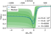 |
Fig. A.1. Impact of the spectral resolution on the PDFs of the transmission function T as a function of input wavelength shift Δλe. We show the PDF of T over all emitters and LOS at z = 3, similarly to Fig. 2. In blue we show the mean for a given Δλe, while in green we show the median. We show the transmission at different spectral resolutions R ∈ {600 000,60 000,6000,1800} (solid, dashed, dotted, dash-dotted). Resolutions below 600 000 are computed as convolution with a Gaussian of FWHM λFWHM that sets the spectral resolution as R = λc/λFWHM. The shaded regions enclose the central 68% of all individual transmission curves. The darkest (lightest) shade corresponds to the lowest (highest) spectral resolution. As the resolution increases the median increases and the shaded region widens. At our fiducial resolution of ∼60 000 these statistics have converged. |
Our simulations at R ∼ 60 000 are expected to be converged due to the Doppler broadening in the line profile. The full width at half maximum (FWHM) due to Doppler broadening is given as  . Assuming an IGM temperature of T ∼ 104 K, this implies a spectral resolution of R ∼ 14 000. Features imprinted by the hydrogen structure on smaller scales will thus be washed out.
The difference in behavior of median and percentiles compared to the mean is easily explained: linearity, that is, STAT[A+B] = STAT[A] + STAT[B] for two distributions, A and B, and a summary statistic, STAT, holds for the mean but not for percentiles such as the median. Take, for example, two PDFs, A = P(T)Δλe = λi and B = P(T)Δλe = λj, where λi and λj describe two neighboring wavelength bins. The mean transmissivity T over those two bins can be determined from the mean of A and B alone, while this is not possible for the median. In particular, if two neighboring bins have the same mean, the mean of the sum of those distributions has to be the same, whereas this is not true for the median, as can be readily seen in Fig. A.1. This behavior is furthermore complicated for the median as the distributions in neighboring bins are strongly correlated. To address this issue, we recommend using the mean transmission curves over the median unless the spectral resolution is clearly stated.
We obtain a triple peak fraction of 28.5%, 28.4%, 17.6%, and 0.1% for spectral resolutions of 600 000, 60 000, 6000, and 1800 given the Gaussian input spectrum. Thus, in addition, the peak count is converged at our fiducial resolution of 60 000. At typical resolutions of spectrographs today (R ∼ 1800), triple peaks are rare to non-existent for given small-scale spectrum.
Appendix B: Start of integration
In Fig. B.1, we vary the start s0 of the integral for the optical depth and show the resulting mean transmission curves. For small changes around s0 = 1.5 ± 1.0rvir, we find the central trough’s depth to slightly change and becoming deeper for smaller values of s0. Going beyond f = 10.0 removes the relevant scale responsible for the mean attenuation curve’s central trough. On an even larger scale (f = 30.0), attenuation is shifted toward lower input wavelengths due to the Hubble flow.
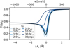 |
Fig. B.1. Impact of the lower integration bound s0 for mean transmission curves. We averaged over all LOS and Lyα- emitting galaxy candidates at z = 3. We show the cases of f = 0.5, 1.0, 2.0, 2.5 around our fiducial case of 1.5. These results are contrasted with cases f = 10.0, 30.0 for interaction on large scales only. In addition, we show the case of a fixed s0 = 30 pkpc irrespective of virial radius of the underlying halo. |
The triple peak count remains stable around ∼30% with 28.9%, 30.2%, 29.4%, 28.2%, and 27.1% for f equal to 0.5, 1.0, 1.5, 2.0, and 2.5 with s0 = frvir. Similarly, when using a constant s0 rather than depending on the virial radius we obtain 29.6% for s0 = 30 pkpc. Thus, our results are robust for chosen f = 1.5.
The peak fraction is largely determined in the proximity of the targeted halo. The triple peak fraction significantly drops to 17.6% and 6.1% for f = 10.0 and f = 30.0, showing that spectra are shaped both in the proximity of emitters (f ≳ 2.5) and on large scales (f ≳ 10.0).
Appendix C: Bimodality of the transmission curves
In Fig. C.1, we show the distribution of transmission coefficients T at fixed input wavelengths Δλe at z = 3.0. We show three different wavelengths: Blue of the line-center (blue line), in the line-center itself (green line), and red of the line-center (red line). The bimodality for the line-center and larger wavelengths is peaking at T zero or unity, while shorter wavelengths show their second peak below unity (∼0.9 here). This second peak’s existence and position is redshift dependent (see main body). We also show the medians (arrows) color coded for the according distribution. For the line-center and redder wavelengths, one peak is commonly so dominant that the median is shifted to there accordingly. While in this case, the median is aligned with one of the peaks, this is not the case for blue wavelengths.
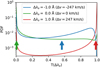 |
Fig. C.1. Distribution of transmission T at fixed input wavelength offset Δλe at z = 3.0 across all emitters and LOS. The arrows show the accordingly color coded median. |
All Figures
|
Fig. 1. Panels showing two different input (i.e., intrinsic) spectra (black lines) and how the IGM attenuation shapes the observed spectra along different LOS at z = 3.0. All spectra are normalized by the respective underlying input spectrum’s total flux. The gray dashed line shows the multiplication of the respective input spectrum with the median transmission curve, |
| In the text | |
|
Fig. 2. PDF of the transmission, T, as a function input wavelength shift, Δλe, over all emitters and the LOS at z = 3. Green line shows the median transmission with the hatched region enclosing the central 68% of all individual transmission curves, while the blue line shows the mean transmission curve over this PDF. The light orange curve shows an example of an individual LOS (corresponding to “LOS 1” in Fig. 1). |
| In the text | |
|
Fig. 3. Evolution of detectable Lyα peaks assuming the three different intrinsic spectra as described in Sect. 2.2. The peak detection algorithm is described in Sect. 3.2.1. |
| In the text | |
|
Fig. 4. Ratios Lratio (top) and Fratio (bottom) shown as a PDF over all lines of sight for both all directions and emitters at a given redshift as shown by the colormap. We chose the double peaked input spectrum, but we also find a very similar result for the centrally peaked input spectrum. The four overplotted lines in each panel show different averaging methods (see text). We assume that no peak can be detected (hence no ratio) when the flux remaining after passing the IGM is less than 1% of the intrinsic flux I(λ). |
| In the text | |
|
Fig. 5. Lratio and Npeaks statistics shown as a function of the large scale overdensity δLSS at redshift z = 4.0. The input spectrum is the Neufeld solution. The colormap in the upper panel shows the underlying PDF normalized at a given δLSS. Overdense regions overall decrease Lratio. At a higher overdensity, this trend halts as the ratio becomes more fluctuating for different LOS. For the peak fractions, we find a gradual decrease of double peaks. This is caused by absorption features on the blue side of the line-center. Thus, the decrease of double peaks is strongly correlated with the increase of the fraction of single peaked spectra. |
| In the text | |
|
Fig. A.1. Impact of the spectral resolution on the PDFs of the transmission function T as a function of input wavelength shift Δλe. We show the PDF of T over all emitters and LOS at z = 3, similarly to Fig. 2. In blue we show the mean for a given Δλe, while in green we show the median. We show the transmission at different spectral resolutions R ∈ {600 000,60 000,6000,1800} (solid, dashed, dotted, dash-dotted). Resolutions below 600 000 are computed as convolution with a Gaussian of FWHM λFWHM that sets the spectral resolution as R = λc/λFWHM. The shaded regions enclose the central 68% of all individual transmission curves. The darkest (lightest) shade corresponds to the lowest (highest) spectral resolution. As the resolution increases the median increases and the shaded region widens. At our fiducial resolution of ∼60 000 these statistics have converged. |
| In the text | |
|
Fig. B.1. Impact of the lower integration bound s0 for mean transmission curves. We averaged over all LOS and Lyα- emitting galaxy candidates at z = 3. We show the cases of f = 0.5, 1.0, 2.0, 2.5 around our fiducial case of 1.5. These results are contrasted with cases f = 10.0, 30.0 for interaction on large scales only. In addition, we show the case of a fixed s0 = 30 pkpc irrespective of virial radius of the underlying halo. |
| In the text | |
|
Fig. C.1. Distribution of transmission T at fixed input wavelength offset Δλe at z = 3.0 across all emitters and LOS. The arrows show the accordingly color coded median. |
| In the text | |
Current usage metrics show cumulative count of Article Views (full-text article views including HTML views, PDF and ePub downloads, according to the available data) and Abstracts Views on Vision4Press platform.
Data correspond to usage on the plateform after 2015. The current usage metrics is available 48-96 hours after online publication and is updated daily on week days.
Initial download of the metrics may take a while.