| Issue |
A&A
Volume 692, December 2024
|
|
|---|---|---|
| Article Number | A98 | |
| Number of page(s) | 9 | |
| Section | Extragalactic astronomy | |
| DOI | https://doi.org/10.1051/0004-6361/202450708 | |
| Published online | 03 December 2024 | |
A resolved Lyman α profile with doubly peaked emission at z ∼ 7
1
Instituto de Astrofísica, Facultad de Física, Pontificia Universidad Católica de Chile, Santiago, 7820436, Chile
2
Las Campanas Observatory, Carnegie Institution of Washington, Casilla 601, La Serena, Chile
3
Instituto de Estudios Astrofísicos, Facultad de Ingeniería y Ciencias, Universidad Diego Portales, Av. Ejército Libertador 441, Santiago, 8370191, Chile
4
Department of Physics and Astronomy, Texas A&M University, College Station, TX 77843-4242, USA
5
George P. and Cynthia Woods Mitchell Institute for Fundamental Physics and Astronomy, Texas A&M University, College Station, TX 77843-4242, USA
6
Astrophysics Science Division, NASA Goddard Space Flight Center, 8800 Greenbelt Road, Greenbelt, Maryland 20771, USA
7
CAS Key Laboratory for Research in Galaxies and Cosmology, Department of Astronomy, University of Science and Technology of China, Hefei, Anhui 230026, People’s Republic of China
8
School of Astronomy and Space Science, University of Science and Technology of China, Hefei, 230026, People ’s Republic of China
9
CAS Key Laboratory for Research in Galaxies and Cosmology, Shanghai Astronomical Observatory, Shanghai, 200030, People’s Republic of China
⋆ Corresponding author; This email address is being protected from spambots. You need JavaScript enabled to view it.
Received:
14
May
2024
Accepted:
5
November
2024
Abstract
Context. The epoch of reionization is a landmark in structure formation and galaxy evolution. How it happened is still not clear, especially regarding which population of objects was responsible for contributing the bulk of ionizing photons to this process. Doubly peaked Lyman-alpha profiles in this epoch are of particular interest since they hold information about the escape of ionizing radiation and the environment surrounding the source.
Aims. We wish to understand the escape mechanisms of ionizing radiation in Lyα emitters during this time and the origin of a doubly peaked Lyman-alpha profile. We also wish to estimate the size of a potential ionized bubble.
Methods. Using radiative transfer models, we fit the line profile of a bright Lyα emitter at z ∼ 6.9 using various gas geometries. The line modeling reveals significant radiation escape from this system.
Results. The studied source shows significant escape (fesc(Lyα) ∼ 0.8, as predicted by the best fitting radiative transfer model) and appears to inhabit an ionized bubble of radius Rb ≈ 0.8−0.3+0.5 pMpc(tage/108)1/3. Radiative transfer modeling predicts the line to be completely redward of the systemic redshift. We suggest the line morphology is produced by inflows, by multiple components emitting Lyα, or by an absorbing component in the red wing.
Conclusions. We propose that CDFS-1’s profile has two red peaks produced by winds within the system. Its high fesc(Lyα) and the low-velocity offset from the systemic redshift suggest that the source is an active ionizing agent. Future observations will reveal whether a peak is present blueward of the systemic redshift or if multiple components produce the profile.
Key words: dark ages / reionization / first stars
© The Authors 2024
 Open Access article, published by EDP Sciences, under the terms of the Creative Commons Attribution License (https://creativecommons.org/licenses/by/4.0), which permits unrestricted use, distribution, and reproduction in any medium, provided the original work is properly cited.
This article is published in open access under the Subscribe to Open model. This email address is being protected from spambots. You need JavaScript enabled to view it. to support open access publication.
1. Introduction
The period following recombination, known as the Dark Ages, was characterized by a neutral intergalactic medium (IGM) and a lack of radiation sources. As structure formed, the first population of stars began to illuminate the cosmos, slowly ionizing the surrounding hydrogen. This process heated the pristine gas around the early galaxies, thus regulating the collapse and formation of new stars. This marked the end of the Dark Ages and the beginning of the epoch of reionization (EoR; Loeb & Barkana 2001; Barkana & Loeb 2001; Furlanetto & Loeb 2005; Benson et al. 2006; Zaroubi 2012).
The EoR is a crucial phase during which most baryonic matter in the Universe, particularly the IGM, became ionized, rendering it transparent to ionizing radiation. While approximate boundaries are known for the onset and conclusion of this epoch, debates persist regarding the specific mechanisms governing the reionization process (Mason et al. 2018). Reionization is commonly described using three parameters that together determine ṅion, the influx of ionizing photons into the IGM. They are: (i) the ultraviolet luminosity density, ρUV, which is closely tied to the number of galaxies hosting hot stars and is typically measured at rest wavelengths of ∼1500 Å; (ii) the ratio of ionizing photon production per UV continuum photon, ξion; and (iii) the fraction of ionizing radiation escaping galaxies to reach the IGM, fesc(LyC) (Robertson et al. 2015). Thus, ̇nion can be written as
 (1)
(1)
The UV luminosity density, ρUV, can be directly determined from the luminosity function (LF) of galaxies observed at the EoR (Bouwens et al. 2015; Donnan et al. 2023; Harikane et al. 2023; Finkelstein et al. 2023). The factor for converting UV photons to ionizing photons, ξion, can be derived from spectroscopic analysis of sources deemed to be similar to high-redshift galaxies (Matthee et al. 2017; Shivaei et al. 2018; Tang et al. 2019). More recently, advances facilitated by the James Webb Space Telescope (JWST) have enabled direct measurements of ξion from sources within the reionization era (Atek et al. 2024; Matthee et al. 2023; Endsley et al. 2023; Prieto-Lyon et al. 2023; Simmonds et al. 2023, 2024a, b; Saxena et al. 2024; Pahl et al. 2024b). However, determining fesc(LyC) poses challenges as residual neutral hydrogen in the IGM absorbs ionizing photons at redshifts z > 4 (Vanzella et al. 2012; Inoue et al. 2014).
The behavior of fesc(LyC) heavily influences models of the reionization history of the Universe (Ishigaki et al. 2018; Finkelstein et al. 2019). Empirical relations have been proposed for fesc(LyC) (Izotov et al. 2016, 2018; Steidel et al. 2018; Matthee et al. 2021; Pahl et al. 2021; Chisholm et al. 2022; Naidu et al. 2022; Pahl et al. 2023, 2024a) and for fesc(Lyα) (Yang et al. 2016; Sobral & Matthee 2019), which correlates with fesc(LyC) (Izotov et al. 2024). Because the geometry of the medium is the main regulator of fesc(LyC), Lyα profiles appear to be one of the most promising proxies for the escape of ionizing radiation given that the two are mediated by the same effects(Verhamme et al. 2006). The radiative transfer of Lyα photons has been thoroughly studied (Neufeld 1990; Ahn et al. 2001, 2002, 2003; Verhamme et al. 2006; Gronke et al. 2015; Li & Gronke 2022), revealing that high escape fractions are associated with low neutral hydrogen column densities (logNHI), low dust optical depths (τdust), and low neutral gas covering fractions (Kakiichi & Gronke 2021; Steidel et al. 2018). Lyα profiles for such systems have undisturbed lines with nonzero flux at rest-frame Lyα wavelengths. In contrast, gas-rich and dusty systems have asymmetric lines with significant offsets with respect to rest-frame Lyα.
Lyman α profiles with flux blueward of the systemic redshift are particularly interesting as they allow for measurements of the separation between peaks. Such systems usually appear as a doublet with zero flux between the blue and red wings, the so-called doubly peaked Lyα profiles; however, in the case of highly efficient radiation escape, the flux between the peaks does not necessarily reach zero (Naidu et al. 2022). At higher redshifts, it has been found that the Lyα line profile is insufficient to infer the fraction of escaping ionizing photons (Pahl et al. 2024a; Choustikov et al. 2024a). However, one can still use it to select potential leakers, as emission near the line center is a necessary condition for high fesc(LyC). In particular, the fraction of Lyα flux close to the systemic redshift (fcen and the Lyα escape fraction seem to be promising proxies at high redshifts; Choustikov et al. 2024b). To date, three sources at redshifts z > 6 with a doubly peaked profile have been reported in the literature (Hu et al. 2016; Songaila et al. 2018; Matthee et al. 2018; Meyer et al. 2021), with significant fesc(LyC) (> 20%) inferred for all of them, as measured from their peaks’ separation. The leading hypothesis as to why the blue wing of the line manages to reach the observer is an ionized bubble scenario in which the sources sit within an ionized hydrogen region with nonzero transmission at wavelengths shorter than 1215.6 Å. Due to the Hubble flow, photons are redshifted as they move through the bubble and are eventually redshifted out of the neutral hydrogen absorption range; thus, it is possible to infer lower limits of the bubble size by measuring the extension of the Lyα blue wing (Mason & Gronke 2020).
Resolving Lyα profiles is still a promising technique for studying the leakage of ionizing radiation at high redshifts; however, technical limitations have made it difficult to carry out these observations. Optical and UV emission lines from EoR sources are observable with JWST. However, its instruments’ spectral resolution cannot resolve the double peaks commonly observed in Lyα profiles (R ∼ 2700 or Δv ∼ 150 km s−1). Ground-based instrumentation is currently the only way to measure the escape of radiation as traced by Lyα profiles.
For these reasons, we have begun a spectroscopic campaign to follow up on the brightest confirmed sources from the Lyman-Alpha Galaxies in the Epoch of Reionization (LAGER) narrowband survey, which aims to study reionization by selecting Lyman alpha emitters (LAEs) at z ∼ 7 to compute the Lyα LF and the clustering of Lyα sources. Medium-resolution spectroscopy with near-infrared coverage allows one to observe both Lyα and nebular emission simultaneously, meaning that we can potentially resolve the Lyα profile and also measure a systemic redshift to constrain the Lyα emission line model.
We present new medium-resolution data of a bright LAE (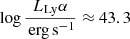 ) from the LAGER survey, namely CDFS-1, first reported in Hu et al. (2019) and followed up on in Yang et al. (2019). We wish to understand the origin of CDFS-1’s doubly peaked Lyman-alpha line and considered different scenarios that can give rise to it.
The paper goes as follows: Section 2 presents observations and data reduction, Sect. 3 the methodology and results, Sect. 4 a discussion, and Sect. 5 the conclusions. Throughout the paper, we use the cosmological parameters from the 2018 Planck results (Planck Collaboration VI 2020): H0 = 67.4 km s−1 Mpc−1 and Ωm = 0.315.
2. Data
2.1. LAGER survey and sample
LAGER is an ongoing project whose aim is to detect ∼600 LAEs at z ∼ 7 across 24 squared degrees. LAGER uses a custom narrowband filter centered on 964 nm mounted on the DECam at the Blanco 4m (Zheng et al. 2017, 2019). Thanks to the combination of a large field of view and near-infrared sensitivity, LAGER has already selected hundreds of LAEs within the EoR and spectroscopically confirmed dozens of them, making it the largest LAE survey at this redshift range (Figs. 1 and 2).
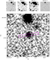 |
Fig. 1. DECam g, i, z, narrowband, and Y stamps centered around CDFS-1. The slit used for the presented observations is drawn in magenta on top of the narrowband stamp. The stamps are 12 arcsec per side. |
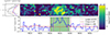 |
Fig. 2. 1D and 2D FIRE spectra Top: Five hours of combined 2D spectra centered around the Lyα line. Bottom: Extracted 1D spectra. We sum all the flux within the columns. We also plot the expected positions of the [OII] and CIII] doublets to show that these lines are not the origin of the observed double peak. Left: Spatial profile of the emission line. We integrate the flux within the shaded region. We also plot only flux integrated blueward (blue) and redward (red) of 9635 Å. |
Being a narrowband survey, the selection is fairly complete for sources with an equivalent width (EW) > 25 Å (Wold et al. 2022). High Lyα EWs have been linked with higher Lyα escape fractions, meaning that LAGER sources were likely ionizing agents during the EoR (Steidel et al. 2018; Sobral & Matthee 2019; Pahl et al. 2021; Flury et al. 2022). Narrowband candidates are selected based on color criteria combined with veto bands; the best candidates are then subjected to spectroscopic follow-up. The spectroscopic confirmation process convolutes the selection functions, as the mask design is a function of candidates’ quality and clustering. Lastly, to study the Lyα profile, the brightest confirmed sources are considered for medium-resolution spectroscopic follow-up, as fainter sources would lead to low-S/N spectra given the increased resolving power.
2.2. Magellan/FIRE spectroscopy
CDFS-1 was observed for a total of five hours on source distributed across the nights of December 12 to 14, 2020, with Magellan/FIRE. FIRE (Simcoe et al. 2013) is a medium-resolution echelle spectrograph mounted on the 6.5m Baade telescope at Las Campanas Observatory. The spectrograph provides simultaneous coverage from 0.8 to 2.5 μm. We used a 0.6 arcsec slit, which yields a resolution of ∼50 km s−1. Each of the 20 exposures is 900s long. The source is nodded along the slit in ABBA cycles followed by an AB cycle of a telluric standard. We defined two positions, “A” and “B”, offset by 2 arcsec; the sources were then observed on position A followed by B. This allows for better sky subtraction. A ThAr lamp was observed between pointings to minimize flexure effects. Each set of four (ABBA) science exposures plus two (AB) telluric exposures is referred to as a block. After discarding non-useful data (e.g., pointing problems, poor conditions), we are left with five blocks totaling 5 hours of exposure time.
2.3. Data reduction
Each block is reduced individually using the FIREHOSE IDL library. We used the fire_addrectified routine to produce rectified 2D spectra of each individual exposure as well as for tellurics. Since no continuum is expected for high-z LAEs, we used custom Python routines to stack individual exposures centered around the telluric’s trace. We first created stacks for each unique block to minimize uncertainties from the separation of CDFS-1 and the telluric star in the image plane; each block stack was visually inspected to determine its position along the spatial direction. We then stacked each block centered around the previously measured position. Lastly, the spectrum was extracted in a 1-arcsecond aperture centered on the emission line.
The next step was to measure the line spread function (LSF) by comparing the width of skylines on our data and the skylines observed with higher resolution instruments (VLT/UVES; Program id:67.A-0278, P.I: López). We turned to the error array of our data, as we expect noise to be dominated by skylines in regions containing them. Thus, the width of the error spikes is similar to that of the skyline producing said noise. Since FIREHOSE creates sky-subtracted data products, we used the error vector to measure the width of skylines.
We started by assuming that both the skylines and their trace on the error vector can be modeled by a Gaussian function; the line width, σlsf, was then computed as
 (2)
(2)
From Eq. (2), we obtain σLSF = 60 km s−1, which is 20% larger than the reported value for the 0.6 arcsec slit.
The point spread function was measured by fitting a Gaussian function to the 2D telluric spectra collapsed in the spectral direction around the wavelength of interest (9634 Å). Consistent with the median seeing of the observing run, we measure a full width at half maximum of 0.6 arcsec.
3. Methodology and results
3.1. Photometric properties
We computed the Lyα luminosity and the Lyα EW by combining DECam’s z-band and narrowband photometry in tandem with the Lyα redshift. The narrowband contains the line flux, while the z-band contains the line flux plus the stellar continuum. The Lyα redshift tells us the filter transmission at the line wavelength. We created synthetic photometric measurements to estimate the uncertainties using the 1σ limiting flux. We report the uncertainties as the 16th and 84th percentile ranges in Table 1.
Physical properties of CDFS-1.
3.2. Line modeling
As done in the literature (Matthee et al. 2018; Hayes et al. 2021), we assumed a systemic redshift such that Lyα falls between the two peaks. The reasoning is that most doubly peaked profiles indeed hold zsys between the peaks (Verhamme et al. 2018). Nevertheless, information on the systemic redshift is necessary to understand the mechanisms behind escaping radiation.
To find the emission line center, the total flux, and most importantly, the blue-to-red (B/R) ratio, we started by fitting two Gaussian functions to our data, as seen in Fig. 3. We fit for the centroid, width, and amplitude of each Gaussian with a Markov chain Monte Carlo (MCMC) approach using the emcee python library (Foreman-Mackey et al. 2013). The MCMC fits two Gaussians with independent widths and centroids simultaneously. The B/R ratio was then computed as the ratio of the areas of each Gaussian, and the systemic redshift was computed from the average wavelengths of the peaks; results are shown in Table 2.
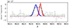 |
Fig. 3. Result from fitting a double Gaussian to the data. The best fit shows a broader blue wing and a narrow red component. The shaded area represents the 16th and 84th percentile results from the MCMC routine. The solid black line is the sum of the two components binned to match the data. |
Results from fitting a double Gaussian model to the Lyα emission line.
To distinguish between a double and a single peak, we computed the Bayesian information criteria (BIC) for a double and single Gaussian, respectively. We then measured the ΔBIC by subtracting the BIC of a double Gaussian from the BIC of a single Gaussian, finding ΔBIC > 10 (Raftery 1995; Szydłowski et al. 2015). There is thus strong evidence in favor of choosing a model with two Gaussians. We then fit a radiative transfer model using FLaREON. FLaREON (Gurung-López et al. 2019) is an open-source Python library that we used to construct models for the following geometries: galactic wind (GW) and thin shell (TS). The models are built from three free parameters for the GW and TS geometries. The FLaREON parameters are the medium expansion velocity (Vexp[km s−1]), the neutral hydrogen column density of the shell (logNHI[cm−2]), which is directly related to the number of scattering events a Lyα photon suffers, and the dust optical depth (logτ), which regulates the number of absorption events. The models are computed from the Orsi et al. (2012) grid of radiative transfer simulations. The medium temperature is fixed at T = 104 K.
FLaREON’s TS model considers a point source surrounded by an isotropic shell of material at a fixed distance from the photon’s origin. Such a configuration can be interpreted as radiation freely traveling before they interact with the ISM and circumgalactic material. Recently, more complex models that incorporate a multiphase medium have been suggested (Kakiichi & Gronke 2021; Li & Gronke 2022). Such models are able to more accurately fit doubly peaked profiles. We note, however, that the S/N presented in this paper limits our capability to distinguish between simple TS models and more sophisticated scenarios.
We fit FLaREON models to our data using the emcee library. Our fitting routine contains five free parameters: the three FLaREON parameters (Vexp, logNHI, and logτ), the systemic redshift, and a scale factor. The goodness of the fit is measured by the reduced χ2 computed from the residuals produced by subtracting each model from the data. Models are convolved with our estimated LSF before subtracting. FLaREON also yields fesc(Lyα) values for each fitted model. This is done by measuring the number of escaping photons divided by the total photon count in the intrinsic spectrum before radiative transfer.
We fit four scenarios: a TS model with a free systemic redshift, a TS model with a fixed systemic redshift computed from the double Gaussian fitting, and a GW model with a free redshift. By doing this, we tested whether CDFS-1 is a bona fide double peak or if its profile arises due to other phenomena. We notice that the GW solution does not present two distinct peaks. We thus disregarded it. The TS model with free systemic redshift offers satisfying solutions. However, when we fixed the redshift to fall between the peaks, we obtained solutions with B/R ratios well below unity. We also used an inflow geometry by mirroring the flux array around the systemic redshift. This inflow geometry allowed us to fit negative velocities (i.e., infalling gas). More details on the models are provided in Gurung-López et al. (2019).
3.3. Comparison with other doubly peaked LAEs
Evidence suggests that CDFS-1 is a doubly peaked LAE at z > 6.5, which would make it the fourth such LAE reported in the literature. To contextualize our results, we subjected the other three sources to the same line modeling analysis. Moreover, we also ran the fitting procedure on KRISS298 (Wofford et al. 2013). KRISS298 is a z ∼ 0.05 LAE with an unusual B/R > 1. By fitting FLaREON models to these four lines, we hoped to validate the models, which would help us interpret the results from CDFS-1. The redshift was left free for all objects, and we adjusted the search range around their reported zLyα.
The models manage to reproduce the doubly peaked nature of COLA-1 and NEPLA-4. KRISS298 is not properly adjusted with an outflow geometry. Instead, an inflow geometry reproduces the observed profile.
The systemic redshift for the three sources is then fitted between the peaks, suggesting that FLaREON is capable of reproducing doubly peaked Lyα profiles. The geometric properties and the Lyα escape fractions are reported in Table 3. We note how all sources show similar logNHI values, and for the high-z sources their logτ are similar as well.
Radiative transfer modeling solutions for two high-redshift (> 6) LAEs and a local LAE with a similar profile as CDFS-1.
Lastly, we note how the velocity offsets from the predicted systemic redshift and the width of the peaks in CDFS-1 are smaller than those of the other LAEs. This can be a signpost of efficient radiation escape, as we discuss in the following sections.
3.4. The bubble surrounding CDFS-1
We wished to extrapolate our findings to the broader population of LAEs at z ∼ 6.9. To do this, we first estimated the size of the ionized bubble surrounding CDFS-1. The equation for a bubble around an isolated ionizing source (ignoring recombination and the Hubble flow) is (Mason & Gronke 2020)
 (3)
(3)
where tage is the timescale the source has been emitting ionizing photons, ̇Nion is the production rate of ionizing photons and  is the mean cosmic hydrogen density at the source’s redshift zs. For the ionizing photon output, ̇Nion, we used Eq. (5) from Yajima et al. (2018):
 (4)
(4)
where ϵLyα = 10.2 eV is the Lyα transition energy. Combining Eqs. (3) and (4), we get the following equation for a bubble of radius Rb:
 (5)
(5)
Izotov et al. (2024) find a tight empirical relation between fesc(Lyα) and fesc(LyC) by studying sources with Lyman continuum measurements of the form
 (6)
(6)
Using our Lyα luminosity, fesc(Lyα), the escape fraction predicted by FLaREON, and zLyα, we obtain Rb ≈ 0.8 pMpc .
.
Then, following a treatment similar to Malhotra & Rhoads (2006), we combined the bubble radius with the number density of Lyα galaxies to derive a volume ionized fraction (XHII). We assumed the same fesc(Lyα) for all LAGER sources, took the volume of a sphere with radius r = Rb, and integrated over the LF to compute XHII. We used the LAE LF from Wold et al. (2022). We integrated the corresponding volume expression for the radius given in Eq. (5) along the LF from L* to ∞, assuming tage = 108, which is on the same order of magnitude as the age of the Universe at z = 6.9
 (7)
(7)
We get a value of XHII ≈ 0.25, meaning that the ionized volume created by bright LAEs is insufficient to fully ionize the Universe.
We note that this is an overestimation of the total ionized volume, as it assumes the same fesc(Lyα) for every source in the LAGER sample and does not take overlap between bubbles into account.
4. Discussion
Yang et al. (2019) presented Magellan/FIRE spectra for CDFS-1 finding no emission lines other than Lyα. The line is slightly/marginally resolved on their lower resolution data, hinting at a doubly peaked emission line profile. The luminosity of CDFS-1  , coupled with its double-peaked profile, hints that this source resides within an ionized region of the Universe (Matthee et al. 2018; Mason & Gronke 2020). Aside from Yang et al. (2019), spectroscopic confirmation of LAGER sources has been presented in Hu et al. (2017), Hu et al. (2021), and Harish et al. (2022). While none of the spectra show a clear signal of a doubly peaked profile, the spectral resolution of the observations is around Δv ∼ 200 km s−1. Figure 2 from Yang et al. (2019) shows CDFS-1 data with a similar resolution and no hints of two peaks. This means that profiles such as the one seen in CDFS-1 might not be uncommon among the parent sample.
4.1. Inference from radiative transfer modeling
The results from various models fitted to CDFS-1 are presented in Table 4, while the results of fitting LAEs in the literature are shown in Table 3. Aside from the properties of the medium, FLaREON is able to compute fesc(Lya), which is presented in Table 1. CDFS-1 is different from the other sources in various aspects; it has an expansion velocity of ∼80 km s−1while the other sources hold small velocities vexp < 20 km s−1. Its peaks are narrower, as seen in Fig. 4, and its predicted systemic redshift does not align with the gap between the peaks. As the expansion velocity increases, the visibility of the blue peak decreases. This happens because photons can escape more easily in the red wing of the profile. However, large values of this parameter would lead to both red peaks merging onto a single wide wing (Verhamme et al. 2006).
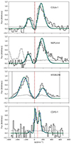 |
Fig. 4. Radiative transfer models for LAEs in the literature. The systemic redshift is fitted between the peaks for every profile except for CDFS-1, suggesting that this source is indeed different from other LAEs. We also note that the peaks in CDFS-1 are visibly narrower than those of its counterparts. Vertical dashed black and red lines mark the zero and the best-fit expansion velocities, respectively. |
Results from fitting FLaREON models to our data.
The narrower peaks seen in CDFS-1 can be attributed to the column density of neutral hydrogen. The column density predicted for CDFS-1 is more than an order of magnitude lower than the rest of the sources. A larger column density leads to a larger number of scattering events prior to escape, leading to photons distributing over a broader range in velocity space. Thus, logNHI regulates both the width and the separation between peaks. We note that Matthee et al. (2018) fitted radiative models to COLA-1, obtaining, logNHI = 17.0, as well as a temperature of LogT = 4.2 and an intrinsic line width of σint = 159 km s−1. Including an intrinsic linewidth and a temperature alleviates the need for higher column densities to reproduce the observed line widths. Thus, we remind the reader that the results from radiative transfer are model dependent and conclusions should only come from comparing sources fitted with the same set of models.
Low-velocity solutions for CDFS-1 are unable to reproduce its B/R ratio, and while negative velocities are able to, they fail to match the width and positioning of the peaks (Fig. 5). As measured by the reduced χ2, the best fit is a Lyα profile with a double red peak. This scenario can reproduce the width, separation, and flux ratios between the peaks. The model predicts a gap at Δv ≈ 70 km s−1, consistent with the expansion velocity of vexp = 70.1 km s−1. This indicates that the expanding medium scatters photons near its Lyα rest-frame wavelength while photons in the “wings” can escape more easily. This interpretation does not present flux blueward of the systemic redshift. However, this does not mean CDFS-1 lacks low-density channels for radiation escape. Its high fesc(Lyα), predicted from either the Lyα EW or the FLaREON solution, coupled with its relatively low Lyα velocity offset, suggest that photons are able to escape the system efficiently.
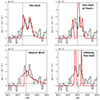 |
Fig. 5. The four models we fit to the data. The best model for each geometry is plotted in red. Using a TS geometry with a free redshift yields the closest matching line profile. Models with a systemic redshift between the two peaks fail to match the narrow separation seen in CDFS-1. The GW geometry fails to reproduce a doubly peaked profile. |
4.2. Origin of the doubly peaked profile
A similar profile has been reported in Tang et al. (2024). The source identified as UDS-07665 shows Lyα emission close to the systemic redshift and fainter red wing separated by ∼100 km s−1. The source also has an EW similar to that of CDFS-1 EW(Lyα) ∼ 100 Å. The line morphology is interpreted as a sign of efficient photon leakage given the high fcen(Lyα), similar to extreme sources such as the sunburst arc (Rivera-Thorsen et al. 2017) and Ion3 (Vanzella et al. 2018). We note that this source possesses a faint blue peak similar to the best-fit FLaREON model; however, the predicted flux is below the noise. We note, however, that UDS-07665 has a central peak at systemic redshift while our best fitting model for CDFS-1 has a peak close to systemic but not at zero velocity. This could be produced by IGM absorption close to the Lyα rest-frame wavelength. If either a peak at the systemic redshift or a clear peak at bluer wavelengths were detected, it would push or estimate of fesc(Lyα) higher as it would more strongly indicate the presence of escape channels within the galaxy.
We considered three scenarios: (a) CDFS-1 has inflows, (b) CDFS-1 contains at least two emitting components, and (c) CDFS-1 is a red wing with an absorption feature. The nature of the system is constrained by its unusually high B/R ratio. Lyα double peak tends to show B/R ratios lower than one, especially at high redshifts where the IGM has a stronger attenuation toward the blue (Laursen et al. 2011; Hayes et al. 2021). Moreover, the IGM absorbs the blue peak even inside ionized bubbles (Tang et al. 2024). Thus, a doubly peaked LAE requires a large bubble size or small separation to be observable. Given the stochasticity of the IGM, we made no attempt to model it in this work and note that an LAE as bright as CDFS-1 is expected to host an ionized bubble. Combined with the fact that the profile is narrow with a small separation, we justify the decision to ignore said component.
Wofford et al. (2013) presented a Lyα double peak with a B/R ratio > 1, which they interpret as infalling gas and is well fitted by our inflow model. Double peaks with B/R > 1 have also been reported in Marques-Chaves et al. (2022), Furtak et al. (2022) and Mukherjee et al. (2023). However, their peak separations are considerably larger than that of CDFS-1. Similarly, Blaizot et al. (2023) shows that profiles with B/R > 1 do emerge in radiative transfer simulations, but once again, the separation between peaks is rarely below Δv ≈ 200 km s−1. Lastly, an inflow scenario seems unlikely given the unsatisfactory fit obtained with the inflow model.
The two peaks could arise from two distinct Lyα emitting regions, which seems even more plausible considering that high-redshift systems tend to be clumpier (for example Fujimoto et al. (2024)). While the two components seen on the 2D spectra are not co-spatial, they are still within the atmospheric full width at half maximum, making their separation smaller than d < 5 kpc. We used that distance in combination with the separation between peaks to estimate the mass of the system, which yielded a value of 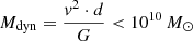 . Were CDFS-1 to be two distinct emitting regions, one would like to distinguish between a merger and a clumpy system. Given the velocity value measured from the separation of the peaks in our double Gaussian fit (∼100 km s−1), a clumpy system appears more feasible. Rest-frame UV observations of high-redshift LAEs reveal highly irregular morphologies. For example, the bright, narrowband-selected z > 6 LAEs CR7 and VR show multiple clumps in the UV while also showing spatial variations in their line profiles (Sobral et al. 2018; Matthee et al. 2019a,b, 2020). Martin et al. (in prep.) present JWST/NIRCam imaging for 10 LAGER-selected LAEs. They find that eight out of the ten imaged sources are resolved into multiple components when observed at JWST’s resolution.
We note a hint of a second component in the z-band broadband data (see Fig. 6). However, just like the spectroscopic data, broadband imaging is limited by atmospheric seeing. Thus, we cannot rule out the possibility of CDFS-1 being an interacting system such as a merger. We propose that the profile seen in CDFS-1 results from an expanding shell, which leaves an absorption feature on the Lyα profile, resulting in a double red peak. However, high-resolution imaging and a systemic redshift are required to rule out inflows and kinematic effects. This is likely a line-of-sight effect, as different sightlines might not hold reservoirs of neutral gas; thus, an absorption feature would not be produced.
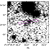 |
Fig. 6. DECam z-band image of CDFS1. We overlay the slit as done in Fig. 1. The morphology appears clumpy. Though one of the components falls outside of the slit, the Lyα-emitting region does not need to be co-spatial with the continuum emitting region. |
4.3. CDFS-1 as an ionizing agent
Assuming the profile emerges from a single system, a doubly peaked Lyα profile with a systemic redshift between the peaks is a signpost of ionizing radiation escape. While this might or might not be true for CDFS-1, the redshift inferred from radiative transfer suggests a Lyα offset of just ∼70 km s−1. Such a small offset is consistent with low-density channels that allow photons to escape undisturbed. This is further supported by the width of the peaks, which are visibly narrower than those of other LAEs. The high Lyα EW is also consistent with low-density channels, as Lyα photons are more sensitive to surrounding neutral hydrogen than continuum photons (Sobral & Matthee 2019; Pahl et al. 2021). Assuming the systemic redshift falls between the peaks, we can measure the minimum extension of the bubble surrounding CDFS-1. Following Matthee et al. (2018), we measure a minimum radius Rmin ≈ 0.2 pMpc for a blue wing extending Δv ≈ 100 km s−1. This value is consistent with the radius computed in Sect. 3.4 as long as tage > 106 consistent with the expected age given the large Lyα EW (Charlot & Fall 1993). This means that CDFS-1 could produce a sufficiently large bubble to allow its blue peak to escape. The three previously known doubly peaked LAEs at z > 6 show comparable minimum radii of Rmin ∼ 0.3 pMpc consistent with the size of the bubbles powered by their Lyα emission (Meyer et al. 2021). Thus, by fixing the systemic redshift between the peaks, one finds that all four of these sources are capable of ionizing their surrounding IGM, which in turn allows for the transmission of the blue peak.
4.4. Hydrogen neutral fraction at z ∼ 7
Assuming all bright LAEs have the same fesc(Lyα) as CDFS-1, we find that they would ionize approximately a quarter of the IGM in the Universe. Figure 7 shows the relation between XHII and fesc(Lyα) in this model. The figure shows that if bright (L > L*) LAEs had Lyα escape fractions close to 1, as is predicted by FLaREON for COLA-1, they would be able to ionize most of the IGM by redshift z = 6.9. The latest LAGER results measure a neutral hydrogen fraction XHII > 0.66 at z ≈ 6.9. Taking into consideration values from other probes, an estimate of XHII > 0.5 is more conservative (Wold et al. 2022). If this volume were ionized exclusively by LAEs, they would require extreme conditions such as fesc(Lyα) close to unity and timescales of tage ∼ 108 years. Moreover, the Lyα luminosity and escape fraction would need to remain constant during the burst period for bubbles to grow. The fesc(Lyα) was likely lower in earlier times, as the first generations of stars are required to carve escape paths for ionizing photons.
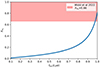 |
Fig. 7. XHII as a function of fesc(Lyα) at a redshift of z ∼ 6.9. We integrate the volume of a bubble across the Lyα LF from L* up to ∞ assuming tage = 108. |
5. Conclusions
We have presented new spectra for CDFS-1, which reveal a doubly peaked profile. However, the profile differs from previously reported z > 6 double peaks. In particular, we find a B/R ratio higher than 1 and a small separation between the peaks of Δv = 95.9 ± 15.6 km s−1. This can be explained if the line morphology is not driven purely by radiative transfer. We propose three scenarios that could give rise to the observed emission: inflating gas, a kinematic effect, and absorption in the red wing of the profile. Out of these scenarios, we consider absorption on the red wing to be the most plausible. Our ground-based observations do not resolve the system into multiple components. Thus, there is no evidence of kinematic effects. For infalling gas, radiative transfer models cannot reproduce the observed profile. However, infalling gas can explain the profile of KRISS298 with a B/R ratio higher than one.
The separation between peaks is considerably smaller than other double peaks observed at redshifts above six. Such a small gap is reproduced via an absorption on the red wing of the profile. The reported double peak does not directly support the theory of an ionized bubble surrounding CDFS-1. While the detection of flux blueward of Lyα signals the presence of an ionized region, the opposite is not true, as a bright LAE can power a surrounding bubble and show no hints of a double peak due to radiative transfer effects. The predicted Lyα escape fractions coupled with the low Lyα velocity offset from the predicted systemic redshift suggest an important contribution of ionizing photons to the neutral IGM. If CDFS-1 were to be a bona fide doubly peaked LAE, the minimum bubble size computed from the line profile (0.2 pMpc) would be consistent with the radius computed from its Lyα luminosity and fesc(Lyα), meaning the source can ionize a bubble large enough for the blue peak to be observed.
Disentangling radiative transfer effects requires a systemic redshift to anchor the rest-frame Lyα wavelength. This would immediately reveal whether CDFS-1 is a doubly peaked LAE with a high B/R ratio and a narrow peak separation or has a profile with two red peaks. The systemic redshift could be obtained from ALMA observations of far-infrared lines or JWST spectroscopy of rest-frame optical emission lines. Moreover, such programs would also provide information about the interstellar medium of ionizing sources during the EoR, allowing comparison with local analogs, as well as potentially reveal neighboring systems that might also be pumping ionizing photons.
To confirm or discard a multicomponent scenario, integral field unit observations and near-infrared imaging are needed in order to resolve the line and continuum emission spatially. Once again, these observations can be achieved with both ALMA and JWST.
Lastly, we show how a population of bright LAEs with extreme Lyα escape fractions (fesc ≈ 1) could ionize the Universe by z ∼ 7 given a long enough starburst period. The fesc(Lyα) is commonly observed to be lower than 1. Furthermore, our calculation assumes that this value and the Lyα luminosity stay constant throughout the 108 year timescale. These requirements suggest that reionization is not solely powered by such sources and that the contribution from other systems, such as fainter LAEs or active galactic nuclei, must be considered.
Future 30-meter class telescopes will be able to resolve the Lyα profile of sources an order of magnitude fainter than what is currently possible. Studying those profiles will shed light on the radiative transfer effects and radiation escape fractions of such systems.
Acknowledgments
CMS acknowledges support from Beca ANID folio 21211528 and support from CATA. This paper includes data gathered with the 6.5-meter Magellan Telescopes located at Las Campanas Observatory, Chile. CMS and LFB acknowledge support from ANID BASAL project FB210003 and FONDECYT grant 1230231, and the China-Chile Joint Research Fund (CCJRF No. 1906). JXW acknowledges support from the science research grant from the China Manned Space Project with No. CMS-CSST-2021-A07. We want to thank Jorryt Matthee and Aida Wofford for sharing their data with us and aiding in the discussion. We also wish to thank the anonymous referee for constructive criticism. Based on observations collected at the European Organisation for Astronomical Research in the Southern Hemisphere under ESO program 67.A-0278.
References
- Ahn, S.-H., Lee, H.-W., & Lee, H. M. 2001, ApJ, 554, 604 [NASA ADS] [CrossRef] [Google Scholar]
- Ahn, S.-H., Lee, H.-W., & Lee, H. M. 2002, ApJ, 567, 922 [NASA ADS] [CrossRef] [Google Scholar]
- Ahn, S.-H., Lee, H.-W., & Lee, H. M. 2003, MNRAS, 340, 863 [Google Scholar]
- Atek, H., Labbé, I., Furtak, L. J., et al. 2024, Nature, 626, 975 [NASA ADS] [CrossRef] [Google Scholar]
- Barkana, R., & Loeb, A. 2001, Phys. Rep., 349, 125 [NASA ADS] [CrossRef] [Google Scholar]
- Benson, A. J., Sugiyama, N., Nusser, A., & Lacey, C. G. 2006, MNRAS, 369, 1055 [NASA ADS] [CrossRef] [Google Scholar]
- Blaizot, J., Garel, T., Verhamme, A., et al. 2023, MNRAS, 523, 3749 [NASA ADS] [CrossRef] [Google Scholar]
- Bouwens, R. J., Illingworth, G. D., Oesch, P. A., et al. 2015, ApJ, 803, 34 [Google Scholar]
- Charlot, S., & Fall, S. M. 1993, ApJ, 415, 580 [Google Scholar]
- Chisholm, J., Saldana-Lopez, A., Flury, S., et al. 2022, MNRAS, 517, 5104 [CrossRef] [Google Scholar]
- Choustikov, N., Katz, H., Saxena, A., et al. 2024a, MNRAS, 529, 3751 [NASA ADS] [CrossRef] [Google Scholar]
- Choustikov, N., Katz, H., Saxena, A., et al. 2024b, MNRAS, 532, 2463 [NASA ADS] [CrossRef] [Google Scholar]
- Donnan, C., McLeod, D., Dunlop, J., et al. 2023, MNRAS, 518, 6011 [Google Scholar]
- Endsley, R., Stark, D. P., Whitler, L., et al. 2023, MNRAS, 524, 2312 [NASA ADS] [CrossRef] [Google Scholar]
- Finkelstein, S. L., D’Aloisio, A., Paardekooper, J.-P., et al. 2019, ApJ, 879, 36 [Google Scholar]
- Finkelstein, S. L., Bagley, M. B., Ferguson, H. C., et al. 2023, ApJ, 946, L13 [NASA ADS] [CrossRef] [Google Scholar]
- Flury, S. R., Jaskot, A. E., Ferguson, H. C., et al. 2022, ApJ, 930, 126 [NASA ADS] [CrossRef] [Google Scholar]
- Foreman-Mackey, D., Hogg, D. W., Lang, D., & Goodman, J. 2013, PASP, 125, 306 [Google Scholar]
- Fujimoto, S., Ouchi, M., Kohno, K., et al. 2024, arXiv e-prints [arXiv:2402.18543] [Google Scholar]
- Furlanetto, S. R., & Loeb, A. 2005, ApJ, 634, 1 [NASA ADS] [CrossRef] [Google Scholar]
- Furtak, L. J., Plat, A., Zitrin, A., et al. 2022, MNRAS, 516, 1373 [NASA ADS] [CrossRef] [Google Scholar]
- Gronke, M., Bull, P., & Dijkstra, M. 2015, ApJ, 812, 123 [Google Scholar]
- Gurung-López, S., Orsi, Á. A., & Bonoli, S. 2019, MNRAS, 490, 733 [CrossRef] [Google Scholar]
- Harikane, Y., Ouchi, M., Oguri, M., et al. 2023, ApJS, 265, 5 [NASA ADS] [CrossRef] [Google Scholar]
- Harish, S., Wold, I. G. B., Malhotra, S., et al. 2022, ApJ, 934, 167 [NASA ADS] [CrossRef] [Google Scholar]
- Hayes, M. J., Runnholm, A., Gronke, M., & Scarlata, C. 2021, ApJ, 908, 36 [Google Scholar]
- Hu, E., Cowie, L., Songaila, A., et al. 2016, ApJ, 825, L7 [NASA ADS] [CrossRef] [Google Scholar]
- Hu, W., Wang, J., Zheng, Z.-Y., et al. 2017, ApJ, 845, L16 [CrossRef] [Google Scholar]
- Hu, W., Wang, J., Zheng, Z.-Y., et al. 2019, ApJ, 886, 90 [NASA ADS] [CrossRef] [Google Scholar]
- Hu, W., Wang, J., Infante, L., et al. 2021, Nat. Astron., 5, 485 [NASA ADS] [CrossRef] [Google Scholar]
- Inoue, A. K., Shimizu, I., Iwata, I., & Tanaka, M. 2014, MNRAS, 442, 1805 [NASA ADS] [CrossRef] [Google Scholar]
- Ishigaki, M., Kawamata, R., Ouchi, M., et al. 2018, ApJ, 854, 73 [NASA ADS] [CrossRef] [Google Scholar]
- Izotov, Y. I., Orlitová, I., Schaerer, D., et al. 2016, Nature, 529, 178 [Google Scholar]
- Izotov, Y. I., Worseck, G., Schaerer, D., et al. 2018, MNRAS, 478, 4851 [Google Scholar]
- Izotov, Y., Thuan, T., Guseva, N., et al. 2024, MNRAS, 527, 281 [Google Scholar]
- Kakiichi, K., & Gronke, M. 2021, ApJ, 908, 30 [CrossRef] [Google Scholar]
- Laursen, P., Sommer-Larsen, J., & Razoumov, A. O. 2011, ApJ, 728, 52 [Google Scholar]
- Li, Z., & Gronke, M. 2022, MNRAS, 513, 5034 [NASA ADS] [CrossRef] [Google Scholar]
- Loeb, A., & Barkana, R. 2001, ARA&A, 39, 19 [NASA ADS] [CrossRef] [Google Scholar]
- Malhotra, S., & Rhoads, J. E. 2006, ApJ, 647, L95 [NASA ADS] [CrossRef] [Google Scholar]
- Marques-Chaves, R., Schaerer, D., Álvarez-Márquez, J., et al. 2022, MNRAS, 517, 2972 [CrossRef] [Google Scholar]
- Mason, C. A., & Gronke, M. 2020, MNRAS, 499, 1395 [Google Scholar]
- Mason, C. A., Treu, T., Dijkstra, M., et al. 2018, ApJ, 856, 2 [Google Scholar]
- Matthee, J., Sobral, D., Best, P., et al. 2017, MNRAS, 465, 3637 [NASA ADS] [CrossRef] [Google Scholar]
- Matthee, J., Sobral, D., Gronke, M., et al. 2018, A&A, 619, A136 [NASA ADS] [CrossRef] [EDP Sciences] [Google Scholar]
- Matthee, J., Sobral, D., Boogaard, L. A., et al. 2019a, ApJ, 881, 124 [NASA ADS] [CrossRef] [Google Scholar]
- Matthee, J., Sobral, D., Gronke, M., et al. 2019b, MNRAS, 492, 1778 [Google Scholar]
- Matthee, J., Pezzulli, G., Mackenzie, R., et al. 2020, MNRAS, 498, 3043 [Google Scholar]
- Matthee, J., Sobral, D., Hayes, M., et al. 2021, MNRAS, 505, 1382 [NASA ADS] [CrossRef] [Google Scholar]
- Matthee, J., Mackenzie, R., Simcoe, R. A., et al. 2023, ApJ, 950, 67 [NASA ADS] [CrossRef] [Google Scholar]
- Meyer, R. A., Laporte, N., Ellis, R. S., Verhamme, A., & Garel, T. 2021, MNRAS, 500, 558 [Google Scholar]
- Mukherjee, T., Zafar, T., Nanayakkara, T., et al. 2023, A&A, 680, L5 [NASA ADS] [CrossRef] [EDP Sciences] [Google Scholar]
- Naidu, R. P., Matthee, J., Oesch, P. A., et al. 2022, MNRAS, 510, 4582 [CrossRef] [Google Scholar]
- Neufeld, D. A. 1990, ApJ, 350, 216 [NASA ADS] [CrossRef] [Google Scholar]
- Orsi, A., Lacey, C. G., & Baugh, C. M. 2012, MNRAS, 425, 87 [NASA ADS] [CrossRef] [Google Scholar]
- Pahl, A. J., Shapley, A., Steidel, C. C., Chen, Y., & Reddy, N. A. 2021, MNRAS, 505, 2447 [NASA ADS] [CrossRef] [Google Scholar]
- Pahl, A. J., Shapley, A., Steidel, C. C., et al. 2023, MNRAS, 521, 3247 [NASA ADS] [CrossRef] [Google Scholar]
- Pahl, A. J., Shapley, A. E., Steidel, C. C., et al. 2024a, arXiv e-prints [arXiv:2401.09526] [Google Scholar]
- Pahl, A. J., Topping, M. W., Shapley, A., et al. 2024b, arXiv e-prints [arXiv:2407.03399] [Google Scholar]
- Planck Collaboration VI. 2020, A&A, 641, A6 [NASA ADS] [CrossRef] [EDP Sciences] [Google Scholar]
- Prieto-Lyon, G., Strait, V., Mason, C. A., et al. 2023, A&A, 672, A186 [NASA ADS] [CrossRef] [EDP Sciences] [Google Scholar]
- Raftery, A. E. 1995, Sociol. Methodol., 25, 111 [CrossRef] [Google Scholar]
- Rivera-Thorsen, T. E., Dahle, H., Gronke, M., et al. 2017, A&AS, 608, L4 [NASA ADS] [CrossRef] [EDP Sciences] [Google Scholar]
- Robertson, B. E., Ellis, R. S., Furlanetto, S. R., & Dunlop, J. S. 2015, ApJ, 802, L19 [Google Scholar]
- Saxena, A., Bunker, A. J., Jones, G. C., et al. 2024, A&A, 684, A84 [NASA ADS] [CrossRef] [EDP Sciences] [Google Scholar]
- Shivaei, I., Reddy, N. A., Siana, B., et al. 2018, ApJ, 855, 42 [Google Scholar]
- Simcoe, R. A., Burgasser, A. J., Schechter, P. L., et al. 2013, PASP, 125, 270 [NASA ADS] [CrossRef] [Google Scholar]
- Simmonds, C., Tacchella, S., Maseda, M., et al. 2023, MNRAS, 523, 5468 [NASA ADS] [CrossRef] [Google Scholar]
- Simmonds, C., Tacchella, S., Hainline, K., et al. 2024a, MNRAS, 527, 6139 [Google Scholar]
- Simmonds, C., Tacchella, S., Hainline, K., et al. 2024b, arXiv e-prints [arXiv:2409.01286] [Google Scholar]
- Sobral, D., & Matthee, J. 2019, A&AS, 623, A157 [NASA ADS] [CrossRef] [EDP Sciences] [Google Scholar]
- Sobral, D., Matthee, J., Brammer, G., et al. 2018, MNRAS, 482, 2422 [Google Scholar]
- Songaila, A., Hu, E. M., Barger, A. J., et al. 2018, ApJ, 859, 91 [Google Scholar]
- Steidel, C. C., Bogosavljević, M., Shapley, A. E., et al. 2018, ApJ, 869, 123 [Google Scholar]
- Szydłowski, M., Krawiec, A., Kurek, A., & Kamionka, M. 2015, Eur. Phys. J. C, 75, 5 [CrossRef] [Google Scholar]
- Tang, M., Stark, D. P., Chevallard, J., & Charlot, S. 2019, MNRAS, 489, 2572 [NASA ADS] [CrossRef] [Google Scholar]
- Tang, M., Stark, D. P., Ellis, R. S., et al. 2024, arXiv e-prints [arXiv:2404.06569] [Google Scholar]
- Vanzella, E., Guo, Y., Giavalisco, M., et al. 2012, ApJ, 751, 70 [NASA ADS] [CrossRef] [Google Scholar]
- Vanzella, E., Nonino, M., Cupani, G., et al. 2018, MNRAS, 476, L15 [Google Scholar]
- Verhamme, A., Schaerer, D., & Maselli, A. 2006, A&A, 460, 397 [NASA ADS] [CrossRef] [EDP Sciences] [Google Scholar]
- Verhamme, A., Garel, T., Ventou, E., et al. 2018, MNRAS, 478, L60 [Google Scholar]
- Wofford, A., Leitherer, C., & Salzer, J. 2013, ApJ, 765, 118 [NASA ADS] [CrossRef] [Google Scholar]
- Wold, I. G., Malhotra, S., Rhoads, J., et al. 2022, ApJ, 927, 36 [NASA ADS] [CrossRef] [Google Scholar]
- Yajima, H., Sugimura, K., & Hasegawa, K. 2018, MNRAS, 477, 5406 [NASA ADS] [CrossRef] [Google Scholar]
- Yang, H., Malhotra, S., Gronke, M., et al. 2016, ApJ, 820, 130 [NASA ADS] [CrossRef] [Google Scholar]
- Yang, H., Infante, L., Rhoads, J. E., et al. 2019, ApJ, 876, 123 [NASA ADS] [CrossRef] [Google Scholar]
- Zaroubi, S. 2012, The First galaxies: Theoretical Predictions and Observational Clues (Springer), 45. [Google Scholar]
- Zheng, Z.-Y., Wang, J., Rhoads, J., et al. 2017, ApJ, 842, L22 [Google Scholar]
- Zheng, Z.-Y., Rhoads, J. E., Wang, J., et al. 2019, PASP, 131, 074502 [NASA ADS] [CrossRef] [Google Scholar]
All Tables
Radiative transfer modeling solutions for two high-redshift (> 6) LAEs and a local LAE with a similar profile as CDFS-1.
All Figures
|
Fig. 1. DECam g, i, z, narrowband, and Y stamps centered around CDFS-1. The slit used for the presented observations is drawn in magenta on top of the narrowband stamp. The stamps are 12 arcsec per side. |
| In the text | |
|
Fig. 2. 1D and 2D FIRE spectra Top: Five hours of combined 2D spectra centered around the Lyα line. Bottom: Extracted 1D spectra. We sum all the flux within the columns. We also plot the expected positions of the [OII] and CIII] doublets to show that these lines are not the origin of the observed double peak. Left: Spatial profile of the emission line. We integrate the flux within the shaded region. We also plot only flux integrated blueward (blue) and redward (red) of 9635 Å. |
| In the text | |
|
Fig. 3. Result from fitting a double Gaussian to the data. The best fit shows a broader blue wing and a narrow red component. The shaded area represents the 16th and 84th percentile results from the MCMC routine. The solid black line is the sum of the two components binned to match the data. |
| In the text | |
|
Fig. 4. Radiative transfer models for LAEs in the literature. The systemic redshift is fitted between the peaks for every profile except for CDFS-1, suggesting that this source is indeed different from other LAEs. We also note that the peaks in CDFS-1 are visibly narrower than those of its counterparts. Vertical dashed black and red lines mark the zero and the best-fit expansion velocities, respectively. |
| In the text | |
|
Fig. 5. The four models we fit to the data. The best model for each geometry is plotted in red. Using a TS geometry with a free redshift yields the closest matching line profile. Models with a systemic redshift between the two peaks fail to match the narrow separation seen in CDFS-1. The GW geometry fails to reproduce a doubly peaked profile. |
| In the text | |
|
Fig. 6. DECam z-band image of CDFS1. We overlay the slit as done in Fig. 1. The morphology appears clumpy. Though one of the components falls outside of the slit, the Lyα-emitting region does not need to be co-spatial with the continuum emitting region. |
| In the text | |
|
Fig. 7. XHII as a function of fesc(Lyα) at a redshift of z ∼ 6.9. We integrate the volume of a bubble across the Lyα LF from L* up to ∞ assuming tage = 108. |
| In the text | |
Current usage metrics show cumulative count of Article Views (full-text article views including HTML views, PDF and ePub downloads, according to the available data) and Abstracts Views on Vision4Press platform.
Data correspond to usage on the plateform after 2015. The current usage metrics is available 48-96 hours after online publication and is updated daily on week days.
Initial download of the metrics may take a while.