SIEGE

F. Calura; R. Pascale; O. Agertz; E. Andersson; E. Lacchin; A. Lupi; M. Meneghetti; C. Nipoti; A. Ragagnin; J. Rosdahl; E. Vanzella; E. Vesperini; A. Zanella

doi:10.1051/0004-6361/202452876

Home

All issues

Volume 698 (May 2025)

A&A, 698 (2025) A207

Full HTML

Open Access

Issue		A&A Volume 698, May 2025


Article Number		A207
Number of page(s)		20
Section		Galactic structure, stellar clusters and populations
DOI		https://doi.org/10.1051/0004-6361/202452876
Published online		20 June 2025

A&A, 698, A207 (2025)

III. The formation of dense stellar clusters in sub-parsec resolution cosmological simulations with individual star feedback

F. Calura¹^★, R. Pascale¹, O. Agertz², E. Andersson³, E. Lacchin⁴^,5^,6, A. Lupi⁷^,8, M. Meneghetti¹, C. Nipoti⁹, A. Ragagnin¹, J. Rosdahl¹⁰, E. Vanzella¹, E. Vesperini¹¹ and A. Zanella¹²^,1

¹ INAF – Osservatorio di Astrofisica e Scienza dello Spazio di Bologna, Via Gobetti 93/3, 40129 Bologna, Italy
² Lund Observatory, Division of Astrophysics, Department of Physics, Lund University, Box 43, 221 00 Lund, Sweden
³ Department of Astrophysics, American Museum of Natural History, New York, NY 10024, USA
⁴ Dipartimento di Fisica e Astronomia “Galileo Galilei”, Università di Padova, Vicolo dell’Osservatorio 3, 35122 Padova, Italy
⁵ INFN – Padova, Via Marzolo 8, 35131 Padova, Italy
⁶ Institut fuer Theoretische Astrophysik, ZAH, Universitaet Heidelberg, Albert-Ueberle-Straße 2, 69120 Heidelberg, Germany
⁷ DiSAT, Università degli Studi dell’Insubria, via Valleggio 11, 22100 Como, Italy
⁸ INFN, Sezione di Milano-Bicocca, Piazza della Scienza 3, 20126 Milano, Italy
⁹ Dipartimento di Fisica e Astronomia “Augusto Righi”, Università di Bologna, Via Gobetti 93/2, 40129 Bologna, Italy
¹⁰ Université Claude Bernard Lyon 1, CRAL UMR5574, ENS de Lyon, CNRS, Villeurbanne 69622, France
¹¹ Department of Astronomy, Indiana University, Bloomington, IN 47401, USA
¹² INAF – Osservatorio Astronomico di Padova, vicolo dell’Osservatorio 5, 35122 Padova, Italy

^★ Corresponding author.

Received: 4 November 2024
Accepted: 3 March 2025

Abstract

Star clusters stand at the crossroads between galaxies and single stars. Resolving the formation of star clusters in cosmological simulations represents an ambitious and challenging goal, since modelling their internal properties requires very high resolution. This paper is the third of a series within the SImulating the Environment where Globular clusters Emerged (SIEGE) project, where we conduct zoom-in cosmological simulations with sub-parsec resolution that include the feedback of individual stars, aimed to model the formation of star clusters in high-redshift proto-galaxies. We investigate the role of three fundamental quantities in shaping the intrinsic properties of star clusters, i.e., (i) pre-supernova stellar feedback (continuous or instantaneous ejection of mass and energy through stellar winds); (ii) star formation efficiency, defined as the fraction of gas converted into stars per freefall time, for which we test 2 different values (ϵ_ff = 0.1 and 1), and (iii) stellar initial mass function (IMF, standard vs top-heavy). All our simulations are run down to z = 10.5, which is sufficient for investigating some structural properties of the emerging clumps and clusters. Among the analysed quantities, the gas properties are primarily sensitive to the feedback prescriptions. A gentle and continuous feedback from stellar winds originates a complex, filamentary cold gas distribution, opposite to explosive feedback, causing smoother clumps. The prescription for a continuous, low-intensity feedback, along with the adoption of ϵ_ff = 1, also produces star clusters with maximum stellar density values up to 10⁴ M_ʘ pc⁻², in good agreement with the surface density-size relation observed in local young star clusters (YSCs). Therefore, a realistic stellar wind description and a high star formation effiency are the key ingredients that allow us to achieve realistic star clusters characterised by properties comparable to those of local YSCs. In contrast, the other models produce too diffuse clusters, in particular the one with a top-heavy IMF.

Key words: methods: numerical / galaxies: formation / galaxies: star clusters: general

© The Authors 2025

Open Access article, published by EDP Sciences, under the terms of the Creative Commons Attribution License (https://creativecommons.org/licenses/by/4.0), which permits unrestricted use, distribution, and reproduction in any medium, provided the original work is properly cited.

This article is published in open access under the Subscribe to Open model. Subscribe to A&A to support open access publication.

1 Introduction

Resolving the formation of star clusters stands out as one of the most ambitious goals in galaxy formation models. Stellar clusters are key to the formation of stars, as increasing evidence suggests that most stars (if not all) are born in various forms of aggregates, such as groups, clusters, or hierarchies of these systems (Lada & Lada 2003; Rodríguez et al. 2020). On the other hand, star clusters strongly affect their surrounding environment through their strong mass and energy outputs, by driving super-bubbles of hot gas that trigger galactic outflows (Tenorio-Tagle et al. 2005; Bik al. 2018; Levy et al. 2021; Orr et al. 2022). Moreover, a large fraction of stars in various galactic components, such as the Milky Way halo and discs, originated from dissolved star clusters (Bica et al. 2001; Wielen 1988; Krumholz et al. 2019; Reina-Campos et al. 2023). Star clusters are often regarded as self-standing entities whose formation, evolution, and possible dissolution were viewed in relative isolation, considering their host galaxy as the background source of a passive tidal field (e.g., Sollima 2021; Vesperini et al. 2021; Lacchin et al. 2024).

Galaxy formation models have frequently described star clusters as macroscopic particles (often called ‘star particles’), typically representing simple stellar populations and ignoring their underlying substructure (e.g., Agertz et al. 2013; Stinson et al. 2013; Hopkins et al. 2018; Feldmann et al. 2023). In current efforts to model the formation and evolution of star clusters within the context of galaxies and cosmology, it has become increasingly clear that this separation between galaxy and star cluster evolution is no longer tenable. As these two are intricately linked, understanding the co-evolution of galaxies and their embedded star clusters has become of crucial importance.

In recent times, thanks to the first observational studies of the progenitors of globular clusters (GCs) at high redshift (Vanzella et al. 2017a,b; Calura et al. 2021; Bouwens et al. 2021; Mowla et al. 2022; Pascale et al. 2023a; Senchyna et al. 2024), star clusters have regained significant interest also from a cosmological perspective. These discoveries motivated several attempts to account for the presence of star clusters in galaxy formation models.

Hydrodynamic simulations performed in a cosmological framework are valuable tools to model realistically several fundamental physical processes, such as the gravitational collapse, radiative cooling and star formation (SF). They are sometimes based on ‘zoom-in’ techniques, in which a low-resolution dark matter (DM)- only simulation is first run, starting from initial conditions computed self-consistently with the adopted cosmology and up to a certain epoch of interest. When a DM halo presents relevant features for the purpose of the study (e.g., it has a suitable virial mass value), higher resolution simulations are then run, centered on that halo and including also the baryonic physics. In most cases, current state-of-the-art simulations reach a spatial resolution that is inadequate to resolve the formation of star clusters in early galaxies. A suitable spatial resolution for this purpose needs to be at a sub-pc scale, sufficient to capture rapid, small-scale key processes such as tidal shocks, as well as the turbulent nature of SF (Renaud et al. 2013; Renaud 2020).

Only a few studies so far have a suitable resolution to investigate the physical conditions in which star clusters originate; however, they suffer from severe limitations. These works resolve the formation of star clusters, although their sizes are generally larger than the observed ones due to limited resolution (Ma et al. 2020). In some very high-resolution simulations of this type, the stellar component is modelled by means of stellar particles, aimed to represent entire stellar populations (Kimm et al. 2016; Garcia et al. 2023). However, the increase in resolution is accompanied by decreasing reliability of the sub-grid description of stars with particles. In paricular, Revaz et al. (2016) showed how below a critical mass particle of 10³ Mʘ, only a direct, star-by-star sampling of the IMF provides a realistic description of the stellar component in hydrodynamic simulations (see also Emerick et al. 2019). Generating individual stars is necessary when the quantity of gas available for SF in a cell is sufficient for a few stars only, which becomes increasingly frequent with sub-pc resolution and gas densities of n∼10³−105 particles cm⁻³, typical of molecular cloud cores. Several simulations describe isolated systems, such as star clusters or galactic systems, in which the stellar component is modelled by means of individual stars that release mass, energy and heavy element in their surroundings (Emerick et al. 2019; Andersson et al. 2020; Lahen et al. 2020; Wall et al. 2020; Gutcke et al. 2021; Hirai et al. 2021; Hu et al. 2023; Deng et al. 2024). In these works, the initial and boundary conditions are idealized or simplified and do not represent the physical complexity of real star-forming systems and their environment, for which the full description of a cosmological framework is required.

The physics of stellar feedback (including stellar winds, supernovae and various radiative processes) sets the amount of mass and energy released by stars into the interstellar medium (ISM) and is a natural consequence of stellar evolution. Within star-forming dense clouds, the timescale on which feedback acts on the system is debated, in particular it is yet unclear whether the most fundamental properties of the system are determined before or after supernova (SN) explosions (e.g., Agertz et al. 2013; Geen et al. 2016; Krumholz et al. 2019; Chevance et al. 2020; Andersson et al. 2024). Another major, unanswered question concerns the role of the star formation efficiency (SFE) and, in particular, how it regulates the formation of bound star clusters (Baumgardt & Kroupa 2007; Grudić et al. 2021; Fukushima & Yajima 2021; Polak et al. 2024). Finally, the number of sources mainly contributing to stellar feedback, i.e. massive stars, is strongly dependent on the IMF, whose shape and evolution is still largely unknown. The roles of these aspects altogether on star cluster formation and their complex interplay have never been addressed in cosmological simulations.

Within a project aimed at SImulating the Environment where Globular clusters Emerged (SIEGE), in a previous work we developed a zoom-in cosmological simulation of a high-redshift dwarf galaxy at sub-pc resolution, including feedback from individual stars (Calura et al. 2022, hereinafter FC22). The model is aimed to describe a strongly lensed star-forming complex observed at z = 6.14 which includes a few star clusters (Vanzella et al. 2019; Calura et al. 2021; Messa et al. 2024).

In their first work, the stellar systems in the simulations of Calura et al. (2022) presented very diffuse stellar clumps, with properties marginally similar to those of high-redshift star forming complexes but significantly different from those of stellar clusters. Building on the model presented in Calura et al. (2022), in the present paper we investigate further this issue and consider how different prescriptions for stellar feedback, SFE and stellar initial mass function impact on star cluster properties, such as density and size.

This paper is organized as follows. In Section 2, we describe the main features of the simulations and the model assumptions. In Sect. 3, we present our results, whereas in Sect. 4 we draw our conclusions. The flat cosmological model adopted throughout this paper has matter density parameter Ωm = 0.276 and Hubble constant H₀ = 70.3 km s⁻¹ Mpc⁻¹ (Omori et al. 2019).

2 Simulations setup

The target of our zoom-in simulations is a DM halo of mass ∼4 × 10¹⁰ M_ʘ at z = 6.14, aimed to represent the host of multiple star-forming clumps, in a system that is the theoretical analogue of the D1-T1 stellar complex, detected through strong gravitational lensing and containing dense stellar systems that qualify as globular cluster precursors (Vanzella et al. 2019; Calura et al. 2021). The cosmological initial conditions are computed as described in FC22. The choice of a comoving volume of 5 Mpc h⁻¹ is key for achieving sub-pc resolution throughout the duration of our simulations, i.e. from z = 100 to z = 10.5. The zoom-in region is defined by means of dark matter-only simulations and a multi-step method, in which we incrementally increase the resolution at intermediate steps (Fiacconi et al. 2017; Lupi et al. 2019; for further details, see FC22). We use the adaptive mesh refinement RAMSES code (Teyssier 2002), that solves the Euler equations with a second-order Godunov method and adopt an HLLC Riemann solver.

In cells eligible for SF, instead of spawing star particles (representing entire stellar populations that sample the full initial mass function, IMF), we stochastically sample the IMF to generate individual stars (Sormani et al. 2017; Calura et al. 2022). Both the stellar and DM components are modelled through collisionless particles, whose trajectories are computed by means of a Particle-Mesh solver. For the DM, the maximum mass resolution is of 200 M_ʘ.

We adopt a quasi-Lagrangian refinement strategy, based on the number of particles present in a cell. Specifically, a cell is refined when its mass exceeds 8 × m_SPH, where m_SPH = 32 M_ʘ. This allows us to reach a maximum physical resolution of 0.2 pc in the densest regions at z = 10.5, corresponding to maximum refinement level lmax = 21. Despite the fact that star clusters are widely known to be fundamentally collisional systems (e.g., Spitzer 1987), in this work we neglect the effects of gravitational collisions between stars. Our choice is justified by recent studies showing that in the long-term evolution of GCs, tidal heating dominates over internal processes, such as stellar collisions (Carlberg & Keating 2022). Addressing the relative roles of the cosmological tidal field and internal processes in the dynamical evolution of star clusters is the focus of an on-going project (Vesperini et al. 2024).

As in FC22, we do not consider any pre-enrichment from population III stars, whose feedback is though to affect the properties of mini-halos at very high redshift and enrich the surrounding intergalactic medium with metals (e.g., Jeon et al. (2017); Klessen & Glover (2023). Investigating their effects is a significant endeavour, as it requires exploring various parameters, including the stellar yields, (e.g., Heger & Woosley 2010), variations in the metallicity transition and initial mass function (Jeon et al. 2017). A study of the effects of individual pop III stars will be the subject of future work.

We present a set of simulations in which we test the effects of various quantities (feedback, stellar initial mass function, star formation efficiency) on the properties of the stellar systems formed in the computational box. A summary of the features of the simulations run in this work is presented in Table 1, useful to illustrate the investigated parameters.

Table 1

Summary of the simulations run in this work.

2.1 Generation of individual stars

In RAMSES (Teyssier 2002), the rate at which gas is converted into new stars is expressed by the Schmidt (1959) law ${\dot{ρ}}_{*} = \frac{ρ}{t_{*}},$ $\dot{\rho}_{\rm *} = \frac{\rho}{t_*},$ (1)

where ρ and ρ_* are the gas and stellar density, respectively, and t_* represents the star formation timescale. This quantity is proportional to the local freefall time $t_{f f} = \sqrt{3 π / 32 G ρ}$ $t_{\rm ff}=\sqrt{3~\pi/32~G \rho}$ and is expressed as $t_{*} = t_{f f} / ϵ_{f f},$ $t_{\rm *}= t_{\rm ff}/\epsilon_{\rm ff},$ (2)

where ∊_ff is the star formation efficiency per freefall time, a fundamental quantity related to the intensity of SF and a free parameter. In the local Universe, SF is known to be an inefficient process, with typical eff values of one or a few percent on the scales of individual giant molecular clouds (GMCs, e.g., Myers et al. 1986; Murray 2011; Federrath & Klessen 2012; Grudić et al. 2019). However, while most observations of GMCs find very similar median values, different surveys suggest a significant spread in _ɛff (Myers et al. 1986; Murray 2011; Evans et al. 2014; Lee et al. 2016; Vutisalchavakul et al. 2016; Utomo et al. 2018; Grudić et al. 2019; Grisdale et al. 2019; see also our Discussion). Deep observations of giant molecular clouds in lensed, star-forming galaxies support higher values for _ɛff at high redshift (Dessauges-Zavadsky et al. 2023), and observations of local starbursts as well (Fisher et al. 2022), where the physical conditions of the star-forming gas are plausibly more similar to the ones of early galaxies (Heckman et al. 1998; Petty et al. 2009; Silverman et al. 2015).

In simulations, ɛ_ff can span 3 order of magnitudes, from a typical value of one or a few percent in galaxy formation simulations aimed to describe the large-scale properties of local galaxies (e.g., Ghodsi et al. 2024; Segovia Otero et al. 2024), up to 100% in works that aim to model globular cluster formation (Li et al. 2018; Brown & Gnedin 2022; Lahén et al. 2023).

In the model of FC22 we assumed ɛ_ff = 0.1, supported by previous results from cosmological simulations of MW-sized galaxies, showing how such choice is consistent with direct observations in molecular clouds and allows one to reproduce fundamentals scaling relations, such as the Kennicutt-Schmidt, and a set of other observables (Agertz & Kravtsov 2015). Later results of isolated MW-like systems suggest that models where star formation is regulated by stellar feedback require ɛ_ff = 0.1 (Grisdale et al. 2019). In this work we test two different SFE values, i.e. ɛ_ff = 0.1 and ɛ_ff = 1.0, and assess their effects on the formation of dense stellar aggregates.

We assume that star formation can occur in cells with gas temperature T < 2 × 10⁴ K. The total mass available for star formation in a cell is split into an array of individual stars using the following method (Sormani et al. 2017). We decompose the stellar mass spectrum into N finite mass intervals. In each interval a mass fraction f_i is defined, so that $\sum_{i = 1}^{N} f_{i} = 1.$ $\sum_{i=1}^{N} f_{i} = 1.$ (3)

In the i-th interval, the number of individual stars n_i is sampled from a Poisson distribution, characterised by a probability P_i given by $P_{i} (n_{i}) = \frac{λ_{i}^{n_{i}}}{n_{i}!} \exp (- λ_{i})$ $P_i(n_i)={\lambda_i^{n_i} \over n_i !} \exp({-\lambda_i}) \,$ (4) where the mean value λ_i is $λ_{i} = f_{i} \frac{M}{m_{i}} .$ $\lambda_i= f_{i} {M \over m_i}.$ (5)

In the equation above, M is the total mass available for star formation (allowing for no more than 90% of the gas in the cell is turned into stars), whereas m_i is the average stellar mass in the i-th bin. We use this formalism to determine the number of individual stars produced in each bin, except for the lowest mass bin, representing stars with mass below 1.5 M_ʘ and where star particles are spawned that collect all the lowest-mass stars together (for further details, see FC22).

To ensure an adequate representation of the IMF, we adopt N = 100 linearly spaced mass bins. In each bin, the calculation of mass fraction f_i requires the assumption of a stellar IMF. The IMF of the first stars is largely unknown and matter of intense debate (e.g., Larson 1998; Glover 2005; Clark et al. 2011; Hirano et al. 2014), as it depends on the interplay of various processes that include (proto-)stellar feedback, metallicity, accretion and gas fragmentation (Bromm & Larson 2004; Ferrara & Salvaterra 2004; Klessen & Glover 2023). In the early Universe, the different chemical composition of the cold gas and, in particular, the absence of heavy elements may affect significantly the radiative cooling and cloud fragmentation, producing an overabundance of massive stars or the formation of extremely massive objects (e.g., Safranek-Shrader et al. 2014; Hirano & Bromm 2017; Chon et al. 2021). Considering this substantial uncertainty, in this work we will test two different choices for the stellar IMF. In most simulations, we assume a Kroupa (2001) (K01) IMF, very common in the local Universe and defined as: $\frac{d n}{d \log m} (m) = {\begin{array}{ll} A \cdot m^{- 0.3} & i f m < 0.5 M_{⊙} \\ B \cdot m^{- 1.3} & i f m \geq 0.5 M_{⊙} . \end{array}$ $\frac{d~n}{d~\log~m} (m) = \Big\{ \begin{array}{l l} A \cdot m^{-0.3} & \qquad {\mathrm{if}} \; m < 0.5 \, \rm M_\odot \\ B \cdot m^{-1.3} & \qquad {\mathrm{if}} \; m \ge 0.5 \, \rm M_\odot. \\ \end{array}$ (6)

The K01 IMF is defined in the mass range 0.1 Μ_ʘ < m < 100 Μ_ʘ. To account for the possible overabundance of massive stars in the early Universe, we also test the effects of a top-heavy IMF (THIMF), for which we consider the simple and convenient functional form $\frac{d n}{d \log m} (m) = c o n s t a n t$ $\frac{d~n}{d~\log~m} (m) = \rm constant$ (7)

(e.g., Jeon et al. 2017) and the same mass range as for the K01. The IMFs adopted in this paper are shown in the top-left panel of Fig. 1. Note that in this plot, the IMF is expressed as $\frac{d n}{d m} (m) = \frac{d n}{d \log m} \frac{1}{m}$ $\frac{d~n}{d~m} (m) = \frac{d~n}{d~\log~m} \frac{1}{m}$ , that is a different conventional way to plot this function and in which the top-heavy IMF is $\frac{d n}{d m} \propto m^{- 1}$ $\frac{d~n}{d~m} \propto m^{-1}$ (in these units, the canonical Salpeter (1955) form is ∝ m^−2.35. Here, we plot the IMFs in the mass range where individual stars are defined, i.e. between ∼1.5 and 100 Μ_ʘ. To maximize the number of stars, the numerical IMFs (black solid and dashed lines) have been calculated at the final times of our simulations.

When generating individual stars, the total stellar mass must not exceed the mass available within the cell. With the exception of a few very rare cases, this causes the truncation of both IMFs at m ∼ 30 Μ_ʘ. Our choice in favor of the conservation of mass causes the loss of a negligible number of massive stars from the total budget, without any significant effect on stellar feedback.

2.2 Stellar feedback prescriptions

We assume that stars in the mass range 8 Μ_ʘ < m < 40 Μ_ʘ contribute to stellar feedback through the release of mass and energy into the ISM in both the pre-SN and SN phases. We test different stellar feedback prescriptions and compare the present results with the ones obtained in the FC22 simulation, where, to model the two phases, all the mass and energy were returned by massive stars instantaneously in two separate episodes, i.e. at their birth and at their death. Since in FC22 we considered 12 mass bins only for the IMF, with a consequent poorer sampling of the stellar mass range, the previous simulations were re-run with the prescriptions described in Sect. 2.1 for a Kroupa (2001) IMF.

In cosmological simulations where star clusters are not resolved, pre-SN feedback has an important role in enhancing the overall effect of stellar feedback. On galactic Scales (e.g., Agertz et al. 2013; Hopkins et al. 2018) momentum injection from stellar radiation, winds and SNe are generally comparable, but SNe (in the post Sedov-Taylor phase) will dominate momentum unless the effect of infrared optical depth is strong (Agertz et al. 2013). However, a few pieces of evidence have suggested that pre-supernova (SN) feedback is fundamental in driving the evolution of young stellar clusters and their surrounding environment (Hopkins et al. 2010; Kruijssen et al. 2019), with SNe explosions expected to play a minor role in key processes, such as the dispersion of gas in molecular clouds (Chevance et al. 2022). Moreover, other studies have shown how the cumulative energy delivered by massive stars in the pre-SN phase is comparable to that released by SN explosions (Castor et al. 1975; Rosen et al. 2014; Calura et al. 2015; Fierlinger et al. 2016). In light of these arguments, in all our simulations, it is crucial to have an adequate description of stellar feedback in the pre-SN phase of massive stars. Through simplified prescriptions, we model the effects of stellar winds from massive stars. In the following, we describe the basic ingredients of our model. In the ‘Winds’ models of this work, in the pre-SN phase and starting immediately after its birth, each massive stars constantly restores mass and energy through a continuous stellar wind. The constant mass and energy return rates are $\dot{M}$ $\dot{M}$ and Ė, respectively, and are proportional to the initial mass m_ini, expressed as $\dot{M} = η \frac{m_{i n i}}{τ_{m}}$ $\dot{M} = \eta \frac{m_{\rm ini}}{\tau_m}$ (8) and $\dot{E} = \frac{\dot{M} v_{w}^{2}}{2} .$ $\dot{E} = \frac{\dot{M} v_w^2}{2}.$ (9)

In Equations (8) and (9), η = 0.45 whereas τ_m is the stellar lifetime, for which we consider the analytic fit of Caimmi (2015) (C15) of the Portinari et al. (1998) results, whereas in Eq. (9) v_w = 2000 km s⁻¹ is the assumed value for the terminal wind velocity (e.g., Weaver et al. 1977; Vink 2018).

Our assumptions concerning the cumulative masses ejected by single stars in the wind phase are consistent with the predictions from stellar evolution models at solar metallicity (Renzo et al. 2017).

We do not assume any dependence of the mass return rate on stellar. We are aware that this assumption is an oversimplifcation, and is likely to lead us to overestimate the effects of stellar winds on the regulation of SF in star clusters (see below).

As in FC22, each massive star ends its life exploding as a SN, returning a fraction η of its initial mass and an amount of thermal energy of 10⁵¹ erg.

The spatial concentration of massive stars can be very large and this can cause extremely large gas temperatures, causing excessively small timesteps in the simulation. To prevent such overheating, we set a maximum value for the temperature (T_max = 10⁸ K) for the hot medium driven by stellar feedback. This value is of the order of the post-shock temperature of the medium energised by stellar winds (Mackey 2023).

As in FC22, we adopt the native, metal-dependent implementation of radiative cooling of the RAMSES code, based on equilibrium-thermochemistry. The cooling and heating rates of the gas are computed as a function of the temperature, density, redshift, metallicity, and the abundances of a set of primordial ion species that include ions of H and He.

To prevent numerical overcooling in high density regions of the ISM, we adopt a delayed cooling scheme as described in FC22. This assumption consists in temporarily switching off cooling in suitable cells, in which the feedback is released as thermal energy. Effective feedback is obtained by assuming that each massive star injects in its cell also an amount of ’nonthermal’ energy, stored in a passive tracer variable and ideally associated with an unresolved, generic turbulent energy. In the native implementation of this scheme (Teyssier et al. 2013), radiative cooling is switched off in each cell in which the local abundance of the ’non-thermal’ passive tracer is above a certain threshold; moreover, the latter is assumed to decay on a dissipation time-scale. As explained in FC22, without any knowledge of the appropriate values for these two quantities and considering also that in the present simulations we model single stars, and not star particles representing entire simple stellar populations, we choose to constrain these two parameters empirically, starting from known recipes from the literature tested at different regimes of mass and spatial resolution (Dubois et al. 2015). By conducting low-resolution tests, we have confirmed that this approach accurately describes stellar feedback and allows us to reproduce the stellar mass of the observed system. On empirical grounds, our choice enables an effective model which allows us to achieve the desired results, i.e. an efficient feedback at our resolution and considering our ingredients.

As for metal production, we adopt the same prescriptions as in FC22. The amount of metals ejected by each single star is described by an analytic formula that represents a polynomial fit to the Woosley & Weaver (1995) stellar yields $y_{Z} = Σ_{k = 1}^{6} f_{k} (m_{i n i} / M_{⊙})^{k}$ $y_{\rm Z} = \Sigma_{k=1}^6 f_k ~ (m_{\rm ini}/\rm M_{\odot})^k$ (10) with f_k = [0.0108, −0.0026,0.00026, −8.81 × 10⁻⁶,1.23 × 10⁻⁷ and −0.5791].

Our prescriptions for stellar feedback are summarised in Fig. 1, where we show the cumulative specific mass (top-right panel), energy (bottom-left panel) and heavy elements mass (bottom-right panel) returned by massive stars in a simple stellar population, calculated assuming a K01 and a top-heavy IMF. In our ‘Winds’ models, the cumulative mass returned by stellar winds and SNe after 30 Myr is equivalent.

Fig. 1 clearly shows how adopting a THIMF causes a stronger energy release. In such case, the cumulative total mass and specific energy returned by a simple stellar population is a factor ∼2 larger than the one obtained with a K01 IMF. The ‘FC22’ model is the one characherised by the largest amount of mass and energy deposited by a newly born stellar population. In fact, it is worth noting that even with a THIMF, the energy deposited soon after the birth, e.g. at 10⁶ yr, is more than one order of magnitude smaller than the one of the FC22 model.

On the other hand, the THIMF causes a considerable enhancement of the cumulative metal fraction, up to a factor ∼3 larger than the K01. This reflects the strong dependence of the metal yields (defined as the specific amount of mass returned by each star in the form of heavy elements) on the initial mass in the prescriptions considered in this work (see FC22).

It is worth noting that stellar mass-loss rates strongly depend on the metallicity and that in stellar evolution models, stellar winds from low-metallicity stars are much weaker during the main sequence phase (e.g., Limongi & Chieffi 2018). In our simulations, a significant fraction of stars are born with zero (or very low) metallicity (Ragagnin et al., in prep.), which, in principle, should have very little effect on star formation. Our assumption of a metallicity-independent prescriptiond for stellar winds leads to overestimating their feedback. This is shown also by the comparison of our prescriptions adopting a K01 IMF and the analytical fits to the metal-dependent cumulative mass loss and energy release estimated by Agertz et al. 2013 (green solid, dashed and dotted lines in Fig. 1), computed from the STARBURST99 code (Leitherer et al. 1999). We are aware that our adoption of metallicity independent rates is an oversimplification that requires improvement. In a forthcoming work, we plan to include metallicity-dependent wind rates (e.g., Dib et al. 2011; Deng et al. 2024) in our models, to study the effects of low-metallicty stellar winds on stellar cluster properties.

Moreover, in general, considering stellar winds as the primary feedback process and neglecting effects form photoionisation radiation represents another oversimplification. In fact, Lancaster et al. (2021b) showed that in dense clouds, turbulent mixing enhances energy losses from the hot interior, and the efficiently-cooled, momentum-driven wind bubbles are not expected to be dominant. In “normal” GMCs (with typical surface density _∑gas ∼ 10² M_ʘ pc⁻²), SF regulation occurs mostly by photoionisation (Kim et al. 2018).

Finally, the progenitors of asymptotic giant branch (AGB) stars are intermediate-mass stars (with a mass m < 8 M_ʘ), which return their ejecta instantaneously at the end of their life. For these stars, we adopt an analytic fit to the final-to-initial stellar mass relation derived by Cummings et al. (2018).

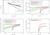Fig. 1

Top-left: stellar IMF computed in this work for a standard (black solid line) and a top-heavy (black dashed line) IMF compared to the analytic ones (cyan solid line: Kroupa (2001); orange dashed line: THIMF). The vertical blue, red and dark-blue dashed lines indicate the minimum mass for individual stars, for massive stars and the maximum mass for SN progenitors, respectively. The top-right is the cumulative mass per unit stellar mass ejected by a stellar population for a Kroupa (2001) (black lines) and top-heavy IMF (red lines) for stellar winds (dashed lines) and SNe (solid lines), whereas the blue dashed line represents the prescriptions for stellar winds ejecta adopted in FC22. The solid, dashed and dotted green straight lines are the metallicity-dependent cumulative mass injected by stellar winds in the model of Agertz et al. (2013) and stopping at t = 6.5 Myr, corresponding to the wind duration in their model. The bottom-left panel is the energy per unit mass and in units of 10⁵¹ erg ejected by stellar winds and SNe in a stellar population, with same line types as in the top-right panel. The bottom-right panel is the specific cumulative mass in the form of heavy elements for a standard (black line) and top-heavy (red line) IMF.

3 Results

In all our simulations, star formation begins at z = 15.95 which, for the adopted cosmology, corresponds to a cosmic time of 0.251 Gyr. In this section, we present our results in the form of slice or projected maps of some relevant quantities that describe the properties of the gas and the stars, computed at three reference, equally spaced redshift values, i. e. z = 15.5, z = 13 and z = 10.5. The choice of running the simulations to z = 10.5 is compliant with the parameter space we aim to explore (see Table 1) and the considerable computational time required by our runs. Moreover, this cosmic time interval is sufficient to gain a clear insight into the properties of the systems formed in our simulations, the differences between the models and the roles played by the most relevant quantities. Most of the results presented in this work concern the central stellar clump, i.e., the stellar aggregate that lies at the centre of the zoom-in region. A more detailed analysis of the general properties of the stellar clumps of the present simulations will be presented in a future study (Pascale et al., in prep.).

3.1 Properties of the star forming gas

The large-scale (i.e. on 1-10 kpc-scale) properties of the starforming gas are not sensitive to the adopted prescriptions regarding feedback implementation, IMF and SFE. Significant differences in the physical properties of the gas are instead visible at the smallest scales probed by our simulations, as seen in Figures 2 and 4, showing zoom slice density maps and projected gravitational pressure maps at various redshifts, respectively, both centered on the central clump of each model.

In the case of the FC22 model, at all redshifts the gas density maps (panels in the left column of Fig. 2) show quite smooth distributions, in particular in the inner regions of each clump, where the amount of visible overdensities and filaments is modest. The adoption of stellar winds in the pre-SN phase (panels in the second column from left) causes a more complicatedly structured density distribution. In particular, at z=15.5, soon after the beginning of SF, the central clump shows a more perturbed distribution than the FC22 model, with a density pattern becoming more and more complex as redshift decreases. This can be appreciated from the amount of filamentary structures which populate the central region.

The new feedback prescriptions adopted here are the key ingredient producing the most remarkable differences with respect to our previous simulations. The maps computed for the SFE=1 and THIMF models do not show appreciable differences with respect to the ‘Winds, SFE=0.1’ model, where a perturbed pattern including a few knots appears already at z = 13. Another remarkable feature is that, in a few cases, each of the three ‘Wind’ models show maximum densities up to ∼10⁻¹⁸ g cm⁻³, significantly larger than the maximum values of the FC22 simulations.

A clearer, quantitative view of the density structure of our simulations can be seen in Fig. 3, where we show the normalised probability distribution function (PDF) of the gas density of the central region extracted from the density maps of Fig. 2, computed for all our models and at different redshifts. Here, the PDF has been computed from the density in each pixel, and the resulting distribution has been normalised to the maximum value. In the FC22 model, at each redshift the density shows a narrow, asymmetric distribution, peaking at large density values (∼10⁻²⁰ g cm⁻³) and with an extended tail running towards low- density values. The ‘Winds’ models (second from top to fourth panel in Fig. 3) show a broader density PDFs and a stronger redshift evolution. In particular, the ‘Winds, SFE=0.1’ model is characterised by a significant shift of the peak density of nearly two orders of magnitude between z = 13 and z = 10.5. All cases show a tail on the right of the peak, that extends to larger maximum density values than the FC22 model. When compared with each other, the distributions of the ‘Winds’ models do not show particularly strong differences, especially at the lowest redshift, z = 10.5, where they peak at similar density values (with a peak at slightly lower density in the ‘Winds, SFE=1’ model). This remarkable change in shape of the PDFs at various redshifts -from narrow to broad distributions while transitioning from the FC22 to the ’Winds’ models- confirms that the stellar feedback prescriptions affect the most the density structure of the starforming gas, weakly affected by other parameters, such as the SFE and the IMF.

In Fig. 4, we report the gravitational pressure of the gas, defined as the gravitational force per unit area $P_{g r a v} = G \times Σ_{g a s}^{2}$ $P_{\rm grav} = G \times \Sigma_{\rm gas}^2$ (Elmegreen & Efremov 1997), where G is the gravitational constant and ∑_gas is the surface density of the gas. In general, in virialised, bound systems like dense clumps or star clusters, the gravitational pressure equals the kinematic pressure, expressed as ρ σ² (where σ is the velocity dispersion, Elmegreen & Efremov 1997; Ma et al. 2020; Calura et al. 2022).

From Fig. 4, we see that from the very beginning (z = 15.5), the gas at the centre of the system is highly pressurized at values P_grav/k > 10⁸ K cm⁻³, typical of the most turbulent local star-forming regions (Sun et al. 2018; Molina et al. 2020). These pressure values correspond to a cloud particle density of 10⁴ cm⁻³ and a turbulent velocity of 10 km/s. For comparison, such values are several orders of magnitudes larger than those of the diffuse, warm ISM in the Milky Way disc, which has typically P_grav/k −10³ K cm⁻³.

One significant difference between the FC22 and the ‘Winds, SFE=0.1’ model is that in the latter, the high-pressure (P_grav/k > 10⁸ K cm⁻³) regions are significantly more compact and showing a complex, filamentary pattern, consisting of multiple small-size knots, at variance with the smoother distribution of the former. It is worth noting that in the ‘Winds, SFE=0.1’, the high pressuregas is distributed more widely than in the FC22 model. At z=10.5 the high pressure-gas distribution reflects the young stars (Fig. 5) and total stellar distribution (Fig. 10). Essentially, more stellar aggregates were born in the ‘Winds, SFE=0.1’ model with respect to the FC22 one, which are more scattered from their birth and that can also undergo significant dynamical interaction, and within which the youngest and most massive stars affect the surrounding gas with their feedback.

At later epochs, the FC22 and the three ‘Winds’ models present maximum values up to P_grav/k ≥ 10⁹ K cm⁻³.

In Figure 4, we also report the 1D density-weighted velocity dispersion of the cold medium (with temperature <200 K), calculated at z = 10.5. This quantity is a measure of the turbulence of the gas and can be defined as: $σ_{1 D}^{2} = \frac{1}{3} \frac{Σ ρ_{c} [(v_{x} - \bar{v_{x}})^{2} + (v_{y} - \bar{v_{y}})^{2} + (v_{z} - \bar{v_{z}})^{2}]}{Σ ρ_{c}}$ $\sigma_{\rm 1D}^2 = \frac{1}{3}\frac{\Sigma \rho_c [(v_x - \bar{v_x})^2 + (v_y - \bar{v_y})^2 + (v_z - \bar{v_z})^2]}{\Sigma \rho_c}$ (11)

(e.g., Shetty et al. 2010; Calura et al. 2020). In Eq. (11), p_c, v_x, v_y and v_z are the density, the x-, y- and z-component of the velocity of the cold gas in a cell respectively, whereas v̄_x, v̄_y and v̄_z are the average x-, y- and z-component velocity values, respectively.

Our results show a factor ∼2 difference in _σ1D between the FC22 and Winds models, a feature that can be ascribed to the stronger feedback that characterises the former.

Moreover, the computed values are very similar in all the ‘Winds’ models, indicating that this quantity is not sensitive to the SFE and IMF, and are of the order of the velocity dispersion measured in local clouds, e.g. as traced by the relation between σ and size observed in molecular clouds (Larson 1981; Elmegreen et al. 2000). The computed values are larger than the thermal velocity dispersion of the cold gas, which is of the order of 1 km/s and corresponding to the sound speed at the considered minimum temperatures (∼ 100 K). This is the signature of a significant degree of turbulence, that does not change significantly with the different prescriptions adopted in our study.

The fundamental reason for the smoother density and pressure maps obtained with the FC22 prescriptions is the stronger, prompt stellar feedback that characterizes this model. In this case, the initial, instantaneous injection of thermal energy coincident with massive star formation wipes away all the small-scale structures in both the density and pressure fields, smoothing out the spatial distributions and creating the homogeneous patterns visible in Figs. 2 and 4.

The properties of the central star-forming regions are illustrated further by the star formation rate (SFR) density maps of Fig. 5, that represents a projected map computed considering the youngest stars at z = 10.5. In each snapshot, we have consider- ered the stars younger than 15 Myr¹ and, in each pixel, computed their cumulative mass and divided it by this time interval and the pixel area. The distribution of young stars in the SFR maps reflects the morphology of the highest pressure regions in Fig. 4. In all cases, the highest SFR values are visible at the centre of the clumps, where the youngest stars can be found.

Additional information on SFR variations in different models is provided in Fig. 6, showing the normalised PDFs of the SFR density in our models, all computed from the ∑_Sfr values in each pixel at z = 10.5. The FC22 and Winds, SFE=0.1/1.0 models show remarkable similarities at the lowest SFR values, Σ_* < 1 M_ʘ yr⁻¹, kpc⁻² and marked differences at larger values. The FC22 model shows a sharp peak at Σ_* ∼ 6-8 M_ʘ yr⁻¹ kpc⁻², whereas the ‘Winds’ models computed with a Kroupa (2001) IMF show more flat-topped distributions. The ‘Winds, SFE=1.0’ shows a broad peak at Σ_* ∼ 10 M_ʘ yr⁻¹ kpc⁻² and extends up to larger values (up to Σ_* > 50 M_ʘ yr⁻¹ kpc⁻²) than its lower- efficiency homologous. On the other hand, a striking feature of the ’Winds, THIMF’ model distribution is that it peaks at a lower Σ_* value (Σ_* ∼ 1 M_ʘ yr⁻¹ kpc⁻²) than the FC22. Moreover, the lowest SFR bins (<0.3 M₀ yr⁻¹ kpc⁻²) are more populated than in all the other cases, underscored by the fact that its normalised distribution shows the highest values in this regime. The star formation history (SFH) of the central region in all our models is illustrated in Fig. A.1, along with the evolution of the cumulative stellar mass obtained in the different cases. This figure is helpful to highlight the regulating effects of stellar feedback on the SFH in the different models.

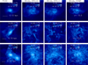Fig. 2

Slice gas density maps in the x-y plane in the four models presented in Table 1 at different redshifts. The maps describe the density distribution in the central region of the simulations in the FC22 (first column from left), ‘Winds, SFE=0.1’ (second), ‘Winds, SFE=1.0’ (third) and ‘Winds, THIMF’ models. The maps are at z = 15.5 (upper row), z = 13 (middle row) and z = 10.5 (bottom row). The horizontal white solid lines shown in the left-hand column-panels indicate the physical scale.

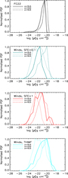Fig. 3

Redshift evolution of the normalised (with respect to the maximum) probability distribution function of the gas density in the same central region of our simulations as in Fig. 2. From top to bottom: gas density PDF in the FC22 (first panel), ‘Winds, SFE=0.1’ (second), ‘Winds, SFE=1.0’ (third) and ‘Winds, THIMF’ (fourth) models at z = 15.5 (solid lines), z = 13 (dotted lines) and z = 10 (dashed lines).

3.2 Properties of the Pre-SN feedback-driven gas

In their pre-SNe phase, massive stars play a fundamental role in determining the physical state of the gas and of the properties of the stellar aggregates. The pre-SN feedback affects the properties of the gas immediately after the formation of new massive stars. On the other hand, SN explosions occur at the end of the stellar lifetimes, therefore SNe of different masses may find diverse gas conditions. In general, SNe of higher masses explode soon after the formation of a new stellar generation. When they explode, the properties of the gas may be closer to the ones of the starforming gas. On the other hand, lower-mass SNe explode later, when the conditions of the gas may be in principle affected by previous explosions. SNe have little effects on the evolution and star formation history of the single clusters. This will be shown in forthcoming works that will address the SFHs of the clusters (Pascale et al. 2025; Ragagnin et al., in prep.).

To investigate further how our prescriptions affect the gas, we study the differences in the physical properties of the medium where SNe explode in various models.

In Fig. 7, we show 2-dimensional temperature-density distributions of the gas where SNe of various masses have exploded in our four different models². The FC22 model shows a narrow distribution, indicating rather similar conditions in which SN explode, with a ∼2 and 4 orders of magnitude dispersion for T and p, respectively. On the other hand, the ‘Winds, SFE=0.1’ model shows a clear anticorrelation that is more similar to typical phase-diagrams of a feedback-driven ISM (Rosdahl et al. 2017; Feldmann et al. 2023; Gurman et al. 2024). The ‘Winds, SFE=0.1’, ‘Winds, SFE=1.0’ and ‘Winds, THIMF’ models show very similar temperature-density distributions, supporting that the change in feedback prescriptions, from the explosive early feedback of FC22 to the more gentle, stellar winds adopted here, plays a stronger role in driving the relation of Fig. 7 than the other parameters.

As already shown in FC22 (see the phase diagrams in Fig. 4 of the supplementary material of Calura et al. 2022), the cold, dense gas with T < 2 × 10⁴ K is promptly turned into new stars. This is the reason why very few SNe explode below this temperature, together with the fact that in the ‘Winds’ models, massive stars heat continuously the gas before the end of their lifetimes. Further information on the SN-driven gas is provided in Fig. 8, illustrating the density of the gas in which SNe of decreasing mass explode. In the FC22 model, SNe explode mostly in relatively dense gas, with the computed distribution peaking slightly below ρ ∼ 10⁻²⁰ g cm⁻³. This is the effect of the long time elapsed between early pre-SN feedback, occurred instantaneously after star formation, and SN explosions, during which the gas is essentially allowed to re-condense and cool. As highlighted by the light-green and blue thick contours, enclosing numbers of SNe corresponding to 60% and 75% of the maximum, respectively, the density range broadens towards lower densities with decreasing mass. This means that, at later times, supernovae can explode under a wider range of physical conditions. This is confirmed also by the left panel of Fig. 9, showing the relation between SN mass and temperature at the explosion, showing a relatively narrow T distribution, peaking at T∼10⁵ K and broadening towards lower masses. The ‘Winds’ models show significantly different distributions in the SN massdensity plane and density PDF as well (shown on the top of each plot in Fig. 8). The ‘Winds, SFE=0.1’ model shows a broad, more symmetric density distribution, with SNe exploding at peak density p ∼ 10⁻²⁴ g cm⁻³, with an overall weaker correlation between mass and density. In the same model, the T distribution of Fig. 9 is strongly asymmetric, due to the fact that SNe cluster at T=10⁸ K, the value chosen for the maximum gas temperature. The saturation at T=10⁸ K also indicates that in this model, the star formation is significantly more concentrated than in the FC22 one. This effect is even stronger for the ‘Winds, SFE=1.0’ model, in which the SN explosion density peaks at about p ∼ 10⁻²⁶ g cm⁻³, i.e. at significantly lower density, whereas the T distribution shows a stronger clustering at T=10⁸ K. This aspect highlights that also the SF efficiency plays an important role in shaping the p and T structure of the feedback-driven gas. Finally, the ‘Winds, THIMF’ is the model that shows the clearest sign of a correlation between exploding SN mass and T, highlighted by the two thick contours in the rightmost panel of Fig. 9. This is the result of the strongest early feedback achieved in this case with respect to the other ‘Winds’ models, in which the final cumulative stellar mass is the lowest (see Table 1 and Fig. A.1), the stars are the least concentrated and where, when the lowest mass SNe explode, the early effects of pre-SNe have weakened the most (although the hint for a similar behaviour is shown also by the ‘Winds, SFE=0.1’ model).

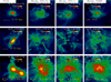Fig. 4

Maps of the gravitational pressure $P_{g r a v} = G Σ_{g a s}^{2}$ $P_{\rm grav} = G\,\Sigma_{\rm gas}^2$ of the gas (see the text for details) in the x-y plane and in the central region of the simulations in the FC22 (first column from left), ‘Winds, SFE=0.1’ (second), ‘Winds, SFE=1.0’ (third) and ‘Winds, THIMF’ (fourth) models. The maps are at z = 15.5 (upper row), z = 13 (middle row) and z = 10.5 (bottom row). The horizontal white solid lines shown in the left-hand column-panels indicate the physical scale. In each panel we report also the 1D density-weighted velocity dispersion of the cold medium (with temperature <200 K) calculated as in Eq. (11).

Fig. 5

Projected SFR surface density maps computed in the x-y plane at z = 10.5 in the central region of the simulations in the FC22 (first panel from left), ‘Winds, SFE=0.1’ (second), ‘Winds, SFE=1.0’ (third) and ‘Winds, THIMF’ (fourth) models.

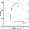Fig. 6

Normalised (with respect to the maximum) probability distribution function of the SFR surface density in the same central region of our simulations as in Fig. 5, at z = 10.5 and in different models. FC22: black solid line; ‘Winds, SFE=0.1’: dotted dark-cyanline; ‘Winds, SFE=1.0’: dashed red line; ‘Winds, THIMF’: dot-dashed lightcyan line.

3.3 Properties of the stellar clumps

The stellar mass density maps of the central region of our simulations at different redshifts is shown in Fig. 10. Starting from the earliest time (z = 15.5), the FC22 model shows a diffuse central clump with a maximum density of 10² M_ʘ pc⁻². At later epochs, the mass and size of the central clumps grows significantly, but the same is not true for the maximum stellar density. At z = 10.5 the stellar clumps show extended and smooth distributions, reflecting the properties of the gas discussed in Sect. 3.1, and with overall sizes of approximately ∼100 pc. At the earliest redshift, the ‘Winds, SFE=0.1’ model does not show significant differences with the FC22, barring a more conspicuous amount of stars, becoming more noticeable at z = 13. At z = 10.5, the ‘Winds, SFE=0.1’ shows more a extended stellar distribution than FC22, with a few dense clumps and a significant amount of diffuse stars. The maximum density values achieved in this model are higher than the FC22 by more than 1 order of magnitude.

On the other hand, the ‘Winds, SFE=1.0’ model shows remarkably high stellar density values already at early times, with two compact stellar clumps clearly visible at z = 15.5. At lower redshift, this model shows some similarities with its lower-SFE homologous, in particular in terms of the extent of the diffuse stellar component but, besides the larger Σ_* values, it also shows a larger abundance of dense aggregates at z = 10.5.

The stellar component in the ‘Winds, THIMF’ model shows intermediate features between the ‘Winds’ and the ‘FC22’ models, with a distribution of diffuse stars similar to the one of the ‘Winds, SFE=0.1’, but with the presence of very few compact knots with maximum densities similar to their counterparts in the FC22 model.

The ‘Winds-THIMF’ model is characterised by a much stronger feedback (i.e. a higher injected specific mass and energy rate, see Fig. 1) than the ‘Winds, SFE=0.1’ and the ‘Winds, SFE=1.0’ models, characterised by a standard Kroupa (2001) IMF. This is the reason for the significantly lower density of the star clusters present in this model.

A few more representative star clusters and clumps in our 4 models are shown in Fig. B.1 and will be discussed in Appendix B.

The normalised PDF of the central surface stellar density at z = 10.5 shown in Fig. 11 (computed as in Fig. 6), helps gaining further insight into the differences between our models. This plot confirms the narrow distribution of the ‘FC22’ model, peaking slightly below Σ_* ∼ 10² M_ʘ pc⁻². The ‘Winds, SFE=0.1’ peaks at a value of Σ_* ∼ 20 M_ʘ pc⁻² but is slightly more populated at the highest values than the ‘FC22’. The ‘Winds, THIMF’ and the ‘Winds, SFE=1.0’ have distributions skewed towards the lowest and highest Σ_* values, respectively. These results confirm that the ‘Winds, SFE=1.0’ model shows the densest stellar aggregates.

Fig. 7

Temperature-density diagrams of the gas in which SNe explode in different models (see the text for further details) in the FC22 (first panel from left), ‘Winds, SFE=0.1’ (second), ‘Winds, SFE=1.0’ (third) and ‘Winds, THIMF’ (fourth) models. The colour scale correspods to the number of SNe exploding in each pixel of the map.

Fig. 8

Density of the gas in which SN explode vs SN progenitor mass in the FC22 (first panel from left), ‘Winds, SFE=0.1’ (second), ‘Winds, SFE=1.0’ (third) and ‘Winds, THIMF’ (fourth) models. The colour scale illustrates the number of SNe exploding in each pixel of the map. The light-blue and blue thick contours enclose numbers of SNe corresponding to 60% and 75% of the maximum, respectively. The histograms on top of each panel are the normalised PDFs of the density.

Fig. 9

Temperature of the gas in which SN explode vs SN progenitor mass in the FC22 (first panel from left), ‘Winds, SFE=0.1’ (second), ‘Winds, SFE=1.0’ (third) and ‘Winds, THIMF’ (fourth) models. The colour scale illustrates the number of SNe exploding in each pixel of the map. The light-orange and red thick contours enclose numbers of SNe corresponding to 60% and 75% of the maximum, respectively. The histograms on top of each panel are the normalised PDFs of the temperature.

3.4 Comparison with the observed young star clusters

In Fig. 12, we analyse a standard scaling relation for young stellar aggregates, the one between stellar surface density and size. In the simulations, the clusters have been identified by means of the Hierarchical Density-Based Spatial Clustering of Applications with Noise (HDBSCAN) software library (McInnes & Healy 2017). HDBSCAN builds a minimum spanning tree (MST) based on the distances of the data points, then it uses a density threshold to build a hierarchy of clusters, set to 25 M_ʘ pc⁻³. This value was chosen on an empirical basis, as we verified that lower values tend to classify non-genuine agglomerates as clusters, while higher values lead to the exclusion of the densest structures. HDBSCAN also requires the expected number of objects per cluster, in our case set to 500, having checked the robustness of the results by varying this parameter across a reasonable range.

For the clustering algorithms, the most common problem is the clump identification in regions that contain diffuse, unbound stellar components. This makes the clump-finding process prone to noise and identification of unreal systems, such as diffuse, extended regions regarded by the software as clumps. The cleaning of the sample from such effects is often troublesome, with automatic procedures not capable of offering reliable solutions. To tackle this aspect, we performed visual inspection of the clumps identified by the algorithm, ensuring that the identified set of clumps is a reliable one and that the rejected clumps were effectively unphysical or classifiable as too diffuse systems.

As for the sizes, in the case of our systems we consider the half-mass radii, computed from the 2D mass density profiles and, for each, calculating the average values along different projections as performed in FC22. In Fig. 12, we show the stellar density (Σ_*³)-size relation for the samples of clusters and clumps identified at z=10.5 in all our models. Although the properties of the star-forming ISM are known to depend critically on redshift (Tacconi et al. 2020), without any observational knowledge of the evolution of the size and mass of young stars clusters across cosmic time, we compare the model properties with an observational dataset of young star clusters from the Legacy Extragalactic UV Survey (Ryon et al. 2017) collected by Brown & Gnedin (2021). The latter is essentially the largest database of local young star clusters (YSCs) radii currently available. In this dataset, the sizes indicated with R_half are the half-light radii.

The clumps obtained in the ‘FC22’ model (black solid squares) are very diffuse and incompatible with local YSCs. The systems identified in the ‘Winds, SFE=0.1’ model (dark-cyan squares) build a diagonal sequence that is partially in agreement with the local sample, yet with too few clusters reaching a density high enough to account for the observational relation of YSCs, populating the upper-left area of the diagram. Moreover, a significant fraction of the clumps identified in the ‘Winds, SFE=0.1’ extend to size values >10 pc and have densities <10 M_ʘ pc⁻², without any observational counterpart. On the other hand, the ‘Winds, SFE=1.0’ model allows us to reproduce nicely the local YSCs relation, as underscored further by the agreement of the linear fits (in log-scales) obtained for the observational data and simulated clusters, represented by the black and red solid lines, respectively.

A comparison between the results of the ‘Winds, SFE=0.1’ (dark cyan squares) and FC22 model (black squares) shows that, for a given IMF, the release of feedback in the form of stellar winds produces significantly denser structures. A comparison between the results of the ’Winds, SFE=1.0’ (red circles) and the ‘Winds, SFE=0.1’ (dark cyan squares) shows that, for the same feedback implementation and IMF, the adoption of a higher SFE produces denser star clusters. The shape of the observational distribution is accounted for, with our ‘Winds, SFE=1.0’ model showing the presence of a few systems with average densities up to several 10³ M_ʘ pc⁻². Still, the less frequent, observed average densities of ∼10⁴−10⁵ M_ʘ pc⁻² shown by some YSCs are not reproduced, and this requires further investigation in future works. Finally, we note that the THIMF model produces the most diffuse clumps, even more diffuse that those obtained in FC22. The result of extremely loose star clusters with a THIMF is the very strong pre-SN feedback characterising this model (Fig. 1), in which the specific cumulative mass and energy for a THIMF (red dotted lines in Fig. 1) are significantly higher than with a K01 IMF, to become comparable to the ones of the ‘Winds, FC22’ model at ∼5-6 Myr and the strongest of all models at later times. This is also the reason of the similarity of the cumulative star formation history of the C22 and THIMF model.

To summarise the results of this Section, the adoption of a high SFE is the key ingredient that allows us to eventually achieve realistic star clusters in our simulations, with properties similar to the ones of local YSCs.

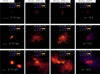Fig. 10

Projected stellar density map in the x-y plane in the four models presented in Table 1 at different redshifts. The maps describe the stellar density in the central region of the simulations in the FC22 (first column from left), ‘Winds, SFE=0.1’ (second), ‘Winds, SFE=1.0’ (third) and ‘Winds, THIMF’ models (fourth column). The maps are at z = 15.5 (upper row), z = 13 (middle row) and z = 10.5 (bottom row). The horizontal white solid lines shown in the left-hand column-panels indicate the physical scale.

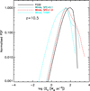Fig. 11

Normalised (with respect to the maximum) probability distribution function of the stellar surface density in the same central region of our simulations as in Fig. 5, at z = 10.5 and in different models. FC22: black solid line; ‘Winds, SFE=0.1’: dotted dark-cyan line; ‘Winds, SFE=1.0’: dashed red line; ‘Winds, THIMF’: dot-dashed lightcyan line.

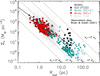Fig. 12

Relation between stellar surface density and size (defined as half-mass or half-light radius) in our simulations and as observed in local star clusters. The black solid squares, dark-cyan solid squares, red solid circles and light-cyan diamonds are the star clusters or clumps retrieved at z = 10.5 in the FC22, ‘Winds, SFE=0.1’, ‘Winds, SFE=1.0’ and ‘Winds, THIMF’ model, respectively, and the small black dots are the observational dataset of young star clusters from the Legacy Extragalactic UV Survey (Ryon et al. 2017; Brown & Gnedin 2021). The thick red and thin black line is a linear fit (in log(∑_*) - log(R_half) space) to the relation found in the ‘Winds, SFE=1.0’ model and in the observational dataset, respectively. Each grey dashed line represents the relation between Σ_* and R_half at fixed stellar mass, for which we have considered various values between 10² M_ʘ and 10⁶ M_ʘ.

4 Discussion

We have shown how both stellar feedback and star formation efficiency play a fundamental role to obtain high-density systems that can be classified as star clusters. In this section, we discuss in more detail these fundamental aspects and the implication of our results in a more general framework, also comparing them with those obtained in other studies.

4.1 Importance of the Pre-SN feedback

Recent studies have shown that early feedback from winds and radiation, occurring before supernova explosions, is necessary to account for some fundamental properties of GMCs, such as the ‘de-correlation’ between molecular gas and young stellar regions at ∼100 pc scales (Chevance et al. 2020). The fact that the co-existence of GMCs and H II regions is very rare on such scales indicates that the evolutionary cycling between GMCs, star formation, and feedback must be rapid and efficient (Krumholz et al. 2019), and that early feedback is the dominant process that drives the destruction of molecular clouds, on typical timescales of a few Myr (Chevance et al. 2020), before the first SN explosions occur.

In the process of pre-SN feedback, the energetic input from massive stars is known to play a crucial role in pre-processing the gas before SNe explode. In fact, while SN explosions are known to dominate the total energy budget on timescales comparable to the lives of massive stars, i.e. up to ∼20-30 Myr (e.g., Fichtner et al. 2022, see also Fig. 1), the pre-SN feedback is of great importance for reducing the circumstellar gas density and limiting radiative losses in SN remnants, strenghtening their impact.

Traditionally, in cosmological simulations pre-SN feedback has often been ignored since it acts on scales much smallerthan the typical maximum resolution (typically >50 pc) that can be achieved in a fully cosmological framework, although a few previous studies have recognised its role, modelled with crude, sub-grid approximations (Hopkins et al. 2011; Stinson et al. 2013; Agertz et al. 2013).

Various pre-SN feedback processes are known to act on scales between ∼1 pc and ∼10 pc (Fichtner et al. 2022 and references therein). These scales can be resolved mostly in non- cosmological simulations, which typically represent isolated systems such as star clusters (e.g., Calura et al. 2015; Yaghoobi et al. 2022) or dwarf galaxies (Agertz et al. 2020; Lahén et al. 2023), where the role of such ingredients can be investigated more carefully. Our results highlight further the importance of pre-SN stellar feedback as a main driver of the early evolution of star clusters. In our previous work, we modelled pre-SN feedback as a local, impulsive release of thermal energy and mass from each newly formed massive star, likely representing an overestimate of its effects and leading to excessively diffuse stellar clumps. In our new simulations, we have shown that the prescription of stellar winds in the form of continuous, slow injection of thermal energy and mass plays a fundamental role in increasing the compactness of the stellar aggregates.

In simulations, the development of the wind-blown bubbles depends crucially on numerical resolution (e.g., Lancaster et al. 2021a). Pittard et al. (2021) discussed the required criteria to inflate a stellar wind bubble in different conditions, such as via momentum and thermal energy injections. In the case of pure thermal energy as in our case, the pressure in the injection region should exceed the environmental one P_amb; this criterion corresponds to a well-defined requirement for the maximum size of the injection region as a function of the mass return rate m and the terminal velocity of the wind v_w: $r_{i n j} = {(\frac{\dot{m} v_{w}}{4 π P_{a m b}})}^{1 / 2} .$ $r_{\rm inj} = \left( \frac{\dot{m} v_w}{4 \pi P_{\rm amb}} \right)^{1/2}.$ (12)

In our case, considering the very high gas density values of >10⁵ cm⁻³ of our star-forming regions and P_amb ∼ ρ T k_B/m_p, a 0.02 pc cell width is required to resolve the wind-driven bubbles, i.e. a factor 10 smaller than our actual resolution at z ∼ 16, therefore we have to recur to our sub-grid, ‘delayed-cooling’ implementation. In other simulations aimed at modelling star cluster formation, stellar feedback is often implemented in the form of momentum injection (Kimm et al. 2016; Li & Gnedin 2019). Despite it has been shown that the clustering of the feedback sources enhances their ɛffects in terms of both momentum and energy (Yadav et al. 2017; Scherer et al. 2018), in most cases for the feedback to be ɛfficient this choice requires the momentum to be artificially boosted by a given factor, that can reach values in excess of 100 even at our resolution (Pittard et al. 2021).

However, we are aware that care needs to be taken when treating stellar winds as the primary feedback process on the typical GMCs scale. In turbulent clouds, most of the energy deposited by stellar winds is dissipated by various processes, including ɛfficient radiative cooling through the mixing between the hot, shocked medium and the colder, surrounding gas (Lancaster et al. 2021a). In such systems, ionising radiation from young massive stars is more ɛffective at regulating SF in the pre-SN phase (Walch et al. 2012; Rosdahl & Teyssier 2015; Geen et al. 2015; Kim et al. 2018). Moreover, also in this case metallicity is expected to have a relevant ɛffect and, according to previous studies of isolated turbulent clouds, it may affect the SFE as well (He et al. 2019).

Although the exact details have not been discussed explicitly, in cosmological simulations this ingredient seems to make a difference even in presence of momentum injection from stellar winds (Kimm et al. 2016; Ma et al. 2020).

In dense environments, also radiation pressure may play an important role in regulating the early phases of star formation in young massive clusters (Fall et al. 2010), even though its regulating ɛffect on GMC scales has been questioned (e.g., Menon et al. 2022).

In the present framework, the contribution of ionising radiation and radiation pressure from individual massive stars remains to be tested, to check how it impacts the star cluster density and whether it requires further artificial assumptions to work, such as momentum boosting; this will be the focus of a future work of the SIEGE series.

4.2 A high star formation efficiency in dense stellar systems

The second important ingredient to achieve dense star clusters is a high SFE. The results of our study indicate that a high SFE, defined as the fraction of gas converted into stars per freefall time ɛ_ff (see Eq. (2)), is needed to reproduce the density values observed in local young star clusters. Considering a density of 10⁵ particles cm⁻³, typical of our star-forming gas, ɛff = 1 corresponds to very fast SF timescales of ∼0.2 Myr. In the present framework, it is important to stress that the SFE is an assumed quantity. The capability to predict a possible range of values for this quantity with an ab-initio approach requires a different type of simulations, including more physical processes, such as magnetohydrodynamics, and spatial resolution down to the AU, currently unfeasible in our conditions, but marginally achievable in studies of isolated SF regions (e.g. Grudic et al. 2019; Polak et al. 2024).

It is worth noting that other definitions of SFE can be found in the literature. A popular one is ɛ, sometimes referred to as the instantaneous SFE $ϵ = \frac{M_{*}}{M_{*} + M_{g a s}},$ $\epsilon = \frac{M_{\rm *}}{M_{\rm *} + M_{\rm gas}},$ (13)

where M_* is the stellar mass and M_gas is the gas mass associated with the star-forming cloud, often represented by the molecular gas and inferred via suitable tracers (Grudić et al. 2019).

Observations suggest that in local star-forming regions, including dense clumps and giant molecular clouds, the SFE can show significant scatter, from a few tenths of percent to a few percent (see Table 2 of Grudić et al. 2019). It is worth noting that the same scatter is shown by both ɛff and ɛ that, in the same set of observations, agree within a factor of ∼2 (Wu et al. 2010; Evans et al. 2014; Heyer et al. 2016; Lee et al. 2016). These measures are performed with different methodologies, that involve tracers of both the stellar (Evans et al. 2014; Heyer et al. 2016; Vutisalchavakul et al. 2016) and molecular gas components (Lada et al. 2010; Wu et al. 2010; Goldsmith & Kauffmann 2017). The reasons for the wide scatter shown by these measures are highly debated and present a serious challenge to modern SF theories (e.g., Hopkins et al. 2014; Grisdale et al. 2019; Segovia Otero et al. 2024). These aim to explain the SFE of molecular clouds based on their turbulent properties, Mach number or virial parameter (Krumholz & McKee 2005; Hennebelle & Chabrier 2011; Padoan & Nordlund 2011; Federrath & Klessen 2012) or balance between gravity and massive stellar feedback (e.g.,Raskutti et al. 2016; Grudić et al. 2018), or to the stochasticity of SF itself, that can account for this huge scatter only up to a limited extent (Grudić et al. 2019). It is also likely that such scatter is intrinsic to the molecular clouds and reflects a strong variation with time of the SFR and gas mass, occurring before the dispersal of the gas (Murray 2011; Feldmann & Gnedin 2011).

At variance with local spirals, observations of star-forming regions in the local, compact starburst galaxy IRAS0 show a two orders-of-magnitude variation in ɛff, reaching extreme values as high as 100% (Fisher et al. 2022) in the central region. This galaxy is located above the local SFR-M, Main sequence where most galaxies lie, therefore, for its intense star formation activity, IRAS0 is regarded as similar to the turbulent, compact starburst galaxies present at high redshift. For some of these systems, separate studies confirm ɛff values higher than local ones (e.g., Dessauges-Zavadsky et al. 2023).

One major, currently unanswered question concerns the physical conditions leading to the formation of bound star clusters, particularly in relation to the SFE.

From the theoretical point of view, a long-standing idea concerns a ‘canonical’ value of ɛ = 50% for the SFE, based on the virial theorem to explain the survival of a bound cluster after mass loss on timescales less than one crossing time (Mathieu 1983). However, in the case of slower gas loss, it is possible for a cluster to survive with lower SFE values (e.g., Boily & Kroupa 2002; Farias et al. 2018.) Other studies have investigated the relation between ɛ and the bound fraction with N-body simulations (e.g., Baumgardt & Kroupa 2007; Shukirgaliyev et al. 2017), showing that ɛ > 30% is required to form gravitationally bound star clusters.

More works based on radiation hydrodynamics simulations showed that in high-density clouds with surface density ∑_gas > 10² M_ʘ pc-², the SFE and the bound fractions can increase significantly due to in ɛfficient photoionisation feedback in a deep gravitational potential (Fukushima & Yajima 2021).

From the observational point of view, the measure of ɛ is more problematic in local young star clusters, in most cases because of the poor available constraints on the amount of cold gas in the systems (Parmentier & Fritze 2009). Exceptions are the bright centres of a few nearby starbursts, that represent the most favourable systems where such measures can be performed. In a few cases, such sites are the hosts of super star clusters, where high SFE values are observed. Through the detection of the J=3-2 rotational CO transition of CO in the local dwarf galaxy NGC 5253, Turner et al. (2015) detected a young, massive (with M^* ∼ 10⁶ M_ʘ) star cluster with ɛ > 50% ɛfficiency. Similar results are found for the SSCs of other systems such as NGC 253, NGC 4945 and Mrk 71A, which present SFE between 50 and 80% (Rico-Villas et al. 2020; Emig et al. 2020; Oey et al. 2017).

Other empirical, sometimes indirect arguments suggest that bound star clusters are likely characterised by high SFE. In particular, arguments related to the dynamics of the gas in clusters, and the response of the surrounding envirnment to the energetic output from massive stars allow one to derive constraints on the SFE (Hills 1980).

In the Milky Way, one of the best studied YMCs is Wester- lund I. At its young age (4.5-5 Myr, Crowther et al. 2006) this system is expected to be out of virial equilibrium because of a recent expulsion of residual gas not converted into stars (Cottaar et al. 2012). One likely explanation for Westerlund I to survive the gas expulsion is a high star-formation ɛfficiency, which would cause the cluster to remain close to virial equilibrium (Mengel & Tacconi-Garman 2009; Cottaar et al. 2012).

Bastian & Goodwin (2006) considered the luminosity profiles of a set of young clusters, with ages <100 Myr and, from the study of their dynamical mass to observed light ratios, found that that several of them were out of virial equilibrium. By means of N-body simulations of clusters including the ɛffects of rapid gas loss, they quantified the ɛffect of rapid gas removal on the cluster disruption, finding that models characterised by SFE between 40% and 50% best reproduced the observed dataset. Hénault-Brunet et al. (2012) studied the dynamical state of the Large Magellanic Cloud young massive cluster R136 through a multi-epoch spectroscopic data analysis of a set of individual stars. From the computed velocity dispersion, they concluded that R136 is in virial equilibrium and, comparing the low velocity dispersion with the values found in a few other young massive clusters, their result suggests that gas expulsion had a negligible ɛffect on its dynamics. Among a few possibilities, this could be explained also with a high star-formation ɛfficiency (Goodwin & Bastian 2006).

In cosmological simulations, an extensive test of the role of the SFE per freefall time on galaxy and cluster properties was performed by Li et al. (2018). In this framework, star clusters are not resolved, but introduced in a sub-grid fashion, where star particles within molecular clouds are allowed to accrete gas from their surroundings. Feedback from new stars can stop this process, and the final particle mass represents the one of a star cluster. While the global galaxy properties were weakly affected by the chosen value of ɛff across a wide range, the cluster properties were rather sensitive to this parameter, in particular the fraction of clustered star formation, showing that to reproduce the increasing observed trend of the cluster formation ɛfficiency with SFR, large values (50-100%) are required. Brown & Gnedin (2022) improved the study of Li et al. (2018), with more comprehensive initial conditions describing more MW- mass progenitors and run down to z=0. Among the explored set of values for ɛff, only ɛff = 1 allows them to reproduce the MW GCs mass function, whereas a too low ɛfficiency of ∼ 1 percent produces too few massive clusters and unrealistic age spreads.

Polak et al. (2024) use high-resolution simulations of turbulent, isolated clouds of various masses where feedback from individual stars is resolved. Their results support that the star formation of YMCs is rapid, with a large fraction (up to 85%) converted into stars within the first freefall time of the collapsing clouds. They stress that an inadequate treatment of feedback from individual stars might lead to overestimating the SFE.

These results highlight the need for additional investigations, possibly within a cosmological framework, to address the interplay of the SFE and stellar feedback, including more physical ingredients such as ionising radiation. In a forthcoming paper, we will study the impact of ionising feedback from individual stars on the self-regulation of SF, in particular testing various values for the SFE.

5 Conclusions

Star clusters represent the building blocks of galaxies and have recently gained interest in galaxy formation. Resolving the formation of star clusters stands out as one of the major ambitions in cosmological simulations, where, due to significant technical challenges and computational limitations, they are often modelled as single particles, whose properties are studied by meansof sub-grid recipes. The study of their internal properties in realistic galactic environments requires high-resolution simulations, most preferably at least at the sub-pc level. Clearly, even such high resolution is not enough to model the formation of single stars, but it is sufficient to quantify how stellar cluster substructures are affected by fast, small-scale gravitational processes such as tidal shocks in the rapidly changing, primordial density field, and to model properly the multi-scale, turbulent nature of star formation. Building upon a previous project aimed at SImulating the Environment where Globular clusters Emerged (SIEGE, Calura et al. 2022; Pascale et al. 2023b), by means of cosmological simulations we studied the roles and the interplay of three fundamental factors, namely (i) stellar feedback, (ii) star formation ɛfficiency and (iii) stellar initial mass function, in shaping the intrinsic properties of star clusters within a cosmological framework. We compared the results obtained in the previous work of FC22, where the pre-SN feedback was modelled through the instantaneous release of a significant quantity of mass and energy by massive stars at their birth, with another model in which stellar winds are implemented, and where massive stars release mass and energy continuously at a low and constant rate. We considered two different models including this feedback scheme, but with two different values for the SFE, expressed as a fraction of the free fall time, i.e. ɛff = 0.1 and ɛff = 1. In one additional model, we matched the stellar winds prescriptions with a top-heavy stellar IMF, characterised by the same mass interval as adopted in the standard case but significantly flatter slope, and therefore more massive stars per stellar mass formed than with the fiducial initial mass function. All the simulations have been run down to z = 10.5, suitable to appreciate the differences between the models and for long enough to characterise the properties of the stellar systems. In the present work, we have focused on the global properties of the simulations, of the structure at the centre of the simulated box and on some star clusters features. In a forthcoming paper we will study in more detail some fundamental scaling relations of the stellar clusters and their evolution on a longer timescale (Pascale et al., in prep.).

Our conclusions can be summarised as follows:

While the large-scale properties of the gas are similar in all simulations, the sub-structural properties of the star-forming clouds are sensitive to the different ingredients considered in our study. At the analysed redshifts, the gas clumps of the FC22 model show a smooth density field. With its gentler release of energy and mass, the adoption of stellar winds is the ingredient making the biggest difference with respect to the old model, as it generates a more perturbed distribution, with the degree of complexity and filamentary structures increasing with decreasing redshift;
This is also supported by the evolution of the gas density PDF. The PDF is narrow in the case of the FC22 model, while it spans a larger range of gas densities in the ‘Winds’ models. The three models with stellar wind prescriptions but different SFE and IMF do not show remarkable differences between each other in either the density maps or the PDFs;
In virialized systems like our clumps, the gravitational pressure P_grav and the 1D density-weighted velocity dispersion. are quantities suited to measure the degree of turbulence. All our models show comparable values of P_grav, although with different morphological distributions. Similar to the gas density, all the ’Winds’ model show filamentary patterns, in particular at late times, regardless of the adopted SFE or IMF. At z = 10.5, all the ’Winds’ models show very similar values for the 1D density-weighted velocity dispersion, a factor ∼2 lower than the value computed for the FC22 model, again to be ascribed to a stronger pre-SN feedback of the latter;
While massive stars start shaping the properties of the ISM immediately after their birth, SNe may find different conditions in the gas in which they explode. In the FC22 model, many SNe explode in gas that had the time to recollapse after the prompt release of energy from newly born massive stars. The ‘Winds’ models show generally a clear anticorrelation between T and p, more similar to typical ISM phase diagrams driven by stellar feedback. The ‘Winds’ model with SFE=0.1 and 1.0 show significant clustering of the feedback sources, that reflects the more compact stellar aggregates;
In comparison with the results of FC22 and adopting the same SFE of 10%, the use of a more gentle pre-SN stellar feedback scheme, characterised by ejection of mass and energy via continuous stellar winds, produces a nearly 2 orders of magnitude increase in the maximum stellar density in the central region of the simulation at z = 10.5. On the other hand, the ‘Winds, SFE=1.0’ model shows remarkably high stellar density already in the earliest phases, with values up to 10⁴ M_ʘ pc⁻² soon after the beginning of star formation. From the analysis of the PDF of the central stellar density across different models at the final redshift of our simulations, the ‘Winds, SFE=1.0’ is the one that shows the distribution skewed towards the highest density values. On the other hand, due to excessive stellar feedback related to the higher number of massive stars, the ‘Winds, THIMF’ is the model characterised by the lowest density in stellar clumps;
We analysed the relation between stellar density (Σ_*) and size for the clusters identified in our models and compared it to observational datasets, incuding both local star clusters and high-redshift clumps. While the observed relation of local star clusters is nicely reproduced by the ‘Winds, SFE=1.0’, all the other models fail in producing dense enough clusters. This confirms that the adoption of a high SF ɛfficiency is the key ingredient that allows us to achieve realistic star clusters, characterised by properties comparable to the ones of local YSCs.

In the future, we will test new ingredients in our models. In particular, we will study the role of ionising radiation on the formation of star clusters and the implications regarding the other quantities analysed here, such as the stellar densities in the most massive star clusters, that sometimes reach values in excess of 10⁵ M_ʘ pc⁻². A follow-up study of early cluster formation in a more massive, Milky-Way mass halo will also be necessary.

Acknowledgements

The research activities described in this paper have been co-funded by the European Union – NextGeneration EU within PRIN 2022 project no. 20229YBSAN - Globular clusters in cosmological simulations and in lensed fields: from their birth to the present epoch. We acknowledge support from the 2023 INAF Mini-Grant ‘Clumps at cosmological distance: revealing their formation, nature, and evolution’ (1.05.23.04.01). This paper is supported by the Fondazione ICSC, Spoke 3 Astrophysics and Cosmos Observations. National Recovery and Resilience Plan (Piano Nazionale di Ripresa e Resilienza, PNRR) Project ID CN_00000013 “Italian Research Center for High-Performance Computing, Big Data and Quantum Computing” funded by MUR Missione 4 Componente 2 Investimento 1.4: Potenziamento strutture di ricerca e creazione di “campioni nazionali di R&S (M4C2-19)” – Next Generation EU (NGEU). EL acknowledges financial support from the European Research Council for the ERC Consolidator grant DEMOBLACK, under contract no. 770017. Enrico Vesperini acknowledges support from NSF grant AST-2009193 and from the John and A-Lan Reynolds Faculty Research Fund. We acknowledge EuroHPC JU for awarding the project IDs EHPC-REG-2021R0052 and EHPC-REG-2024R01- 042 access to DISCOVERER at the Sofia Tech Park, Bulgaria. This research wassupported in part by Lilly Endowment, Inc., through its support for the Indiana University Pervasive Technology Institute.

Appendix A Star formation history of the central clump

To better understand the differences in the features of our models, in this Section we analyse the SFHs calculated in the central regions of the box and shown in Figs. 2, 4, 5, 10. In the upper and lower panels of Fig. A.1 we show the evolution of the star formation rate and the cumulative stellar mass, respectively, of the central regions of the box for the 4 models considered in this work. The model with the most massive central clump at z = 10.5 is the ’Winds, SFE=1.0’, characterised by M_* = 3 × 10⁶M_ʘ. By comparing the results of the ’Winds, SFE=0.1’ and ’Winds, SFE=1.0’ models, it is interesting to note that a factor 10 increase in the SFH results in a factor ∼2 increase in the final stellar mass at z = 10.5. Despite significant differences in both the feedback implementation and adopted IMF, another important aspect is the remarkable similarity between the cumulative stellar mass shown by the ’FC22’ and ’Winds, THIMF’. The final cumulative stellar mass of the ’Winds, SFE=1.0’ model is a factor ∼2, 3.1 and 4.3 higher than the one of the ’Winds, SFE=0.1’, ’FC22’ and ’Winds, THIMF’, respectively.

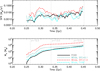Fig. A.1

Star formation history of the central regions of the box (see Figs. 2 and 10) in the models considered in the present work. In the upper and lower panel we show the evolution of the SFR and the cumulative stellar mass, respectively, obtained in the ‘FC22’ (black solid line), ‘Winds, SFE=0.1’ (dark-cyan solid line), ‘Winds, SFE=1.0’ (red solid line) and ‘Winds, THIMF’ (solid cyan line). The three vertical dashed lines represent the cosmic times of the snapshots considered in this works, for which we report the corresponding redshifts.

Appendix B A few dense star clusters and clumps

In Fig. B.1 we show the stellar density maps for some representative clumps and clusters of each model. This figure highlights further the different features of the stellar aggregates created in our simulations. Very diffuse, extended clumps are formed within the ’FC22’ model (first colums from left of Fig. B.1). The change of prescriptions from the ’FC22’ model, characterised by instantaneous and intense release of energy and mass in the pre-SN phase, to the low-intensity stellar winds of the ’Winds, SFE=0.1’ model leads to a major transition from extended clumps to very compact star clusters, with maximum densities larger by one order of magnitude or more (second column).

By adopting a factor 10 higher SFE ɛfficiency, in the ’Winds, SFE=1.0’ model the cluster densities may reach values up to 10⁴ M_ʘ pc⁻² and sizes of the order of ∼1 pc (third column). Finally, again due to the stronger feedback, the clumps of the ’Winds, THIMF’ model (fourth column) are characterised by extended, scattered stellar distributions with compact knots at their centre, but presenting significantly lower maximum densities, of Σ_* ∼ 10² M_ʘ pc⁻².

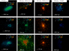Fig. B.1

Projected stellar density maps in the x-y plane for a few representative stellar clumps and star clusters in our models at z = 10.5. Starting from the left, in the first, second, third and fourth column we show clumps or clusters in the ’FC22’, ’ Winds, SFE=0.1’, ’Winds, SFE=1.0’ and ’Winds, THIMF’ model, respectively. The horizontal white solid lines shown in each panel indicates the physical scale.

References

Agertz, O., & Kravtsov, A. V. 2015, ApJ, 804, 18 [NASA ADS] [CrossRef] [Google Scholar]
Agertz, O., Kravtsov, A. V., Leitner, S. N., & Gnedin, N. Y. 2013, ApJ, 770, 25 [NASA ADS] [CrossRef] [Google Scholar]
Agertz O., Pontzen, A., Read, J. I., et al. 2020, MNRAS, 491, 1656 [Google Scholar]
Andersson, E. P., Agertz, O., & Renaud, F. 2020, MNRAS, 494, 3328 [NASA ADS] [CrossRef] [Google Scholar]
Andersson, E. P., Mac Low, M.-M., Agertz, O., Renaud, F., & Li, H. 2024, A&A, 681, A28 [NASA ADS] [CrossRef] [EDP Sciences] [Google Scholar]
Arzoumanian, D., André, P., Didelon, P., et al. 2011, A&A, 529, L6 [NASA ADS] [CrossRef] [EDP Sciences] [Google Scholar]
Bastian, N., & Goodwin, S. P. 2006, MNRAS, 369, L9 [NASA ADS] [CrossRef] [Google Scholar]
Baumgardt, H., & Kroupa, P. 2007, MNRAS, 380, 1589 [NASA ADS] [CrossRef] [Google Scholar]
Bica, E., Santiago, B. X., Dutra, C. M., et al. 2001, A&A, 366, 827 [NASA ADS] [CrossRef] [EDP Sciences] [Google Scholar]
Bik, A., Ostlin, G., Menacho, V., et al. 2018, A&A, 619, A131 [NASA ADS] [CrossRef] [EDP Sciences] [Google Scholar]
Boily, C., & Kroupa, P. 2002, ASPC, 285, 141 [Google Scholar]
Bouwens, R. J., Illingworth, G. D., van Dokkum, P. G., et al. 2021, AJ, 162, 255 [NASA ADS] [CrossRef] [Google Scholar]
Bromm, V., & Larson, R. B. 2004, ARA&A, 42, 79 [NASA ADS] [CrossRef] [Google Scholar]
Brown, G., & Gnedin, O. Y. 2021, MNRAS, 508, 5935 [NASA ADS] [CrossRef] [Google Scholar]
Brown, G., & Gnedin, O. Y. 2022, MNRAS, 514, 280 [Google Scholar]
Caimmi, R. 2015, arXiv e-prints [arXiv:1504.07730] [Google Scholar]
Calura, F., Few, C. G., Romano, D., & D’Ercole, A. 2015, ApJ, 814, L14 [NASA ADS] [CrossRef] [Google Scholar]
Calura, F., Bellazzini, M., & D’Ercole, A. 2020, MNRAS, 499, 5873 [Google Scholar]
Calura, F., Vanzella, E., Carniani, S., et al. 2021, MNRAS, 500, 3083 [Google Scholar]
Calura, F., Lupi, A., Rosdahl, J., et al. 2022, MNRAS, 516, 5914 [Google Scholar]
Calzetti, D., Lee, J. C., Sabbi, E., et al. 2015, AJ, 149, 51 [Google Scholar]
Carlberg, R. G., & Keating, L. C. 2022, ApJ, 924, 77 [NASA ADS] [CrossRef] [Google Scholar]
Castor, J., McCray, R., & Weaver, R. 1975, ApJ, 200, L107 [NASA ADS] [CrossRef] [Google Scholar]
Chevance, M., Kruijssen, J. M. D., Vazquez-Semadeni, E., et al. 2020, SSRv, 216, 50 [Google Scholar]
Chevance, M., Kruijssen, J. M. D., Krumholz, M. R., et al. 2022, MNRAS, 509, 272 [Google Scholar]
Chon, S., Omukai, K., & Schneider, R. 2021, MNRAS, 508, 4175 [NASA ADS] [CrossRef] [Google Scholar]
Clark, P. C., Glover, S. C. O., Klessen, R. S., & Bromm, V. 2011, ApJ, 727, 110 [NASA ADS] [CrossRef] [Google Scholar]
Cottaar, M., Meyer, M. R., Andersen, M., & Espinoza, P. 2012, A&A, 539, A5 [NASA ADS] [CrossRef] [EDP Sciences] [Google Scholar]
Crowther, P. A., Hadfield, L. J., Clark, J. S., Negueruela, I., & Vacca, W. D. 2006, MNRAS, 372, 1407 [Google Scholar]
Cummings, J. D., Kalirai, J. S., Tremblay, P.-E., Ramirez-Ruiz, E., & Choi, J. 2018, ApJ, 866, 21 [NASA ADS] [CrossRef] [Google Scholar]
Deng, Y., Li, H., Liu, B., et al. 2024, A&A, 691, A231 [NASA ADS] [CrossRef] [EDP Sciences] [Google Scholar]
Dessauges-Zavadsky, M., Richard, J., Combes, F., et al. 2023, MNRAS, 519, 6222 [NASA ADS] [CrossRef] [Google Scholar]
Dib, S., Piau, L., Mohanty, S., & Braine, J. 2011, MNRAS, 415, 3439 [NASA ADS] [CrossRef] [Google Scholar]
Dubois, Y., Volonteri, M., Silk, J., et al. 2015, MNRAS, 452, 1502 [Google Scholar]
Elmegreen, B. G., & Efremov, Y. N. 1997, ApJ, 480, 235 [Google Scholar]
Elmegreen, B. G., Efremov, Y., Pudritz, R. E., & Zinnecker, H. 2000, Protostars and Planets IV, 179 [Google Scholar]
Emerick, A., Bryan, G. L., & Mac Low, M.-M. 2019, MNRAS, 482, 1304 [NASA ADS] [CrossRef] [Google Scholar]
Emig, K. L., Bolatto, A. D., Leroy, A. K., et al. 2020, ApJ, 903, 50 [NASA ADS] [CrossRef] [Google Scholar]
Evans, N. J., Heiderman, A., & Vutisalchavakul, N. 2014, ApJ, 782, 114 [CrossRef] [Google Scholar]
Fall, S. M., Krumholz, M. R., & Matzner, C. D. 2010, ApJ, 710, L142 [NASA ADS] [CrossRef] [Google Scholar]
Farias, J. P., Fellhauer, M., Smith, R., Domínguez, R., & Dabringhausen, J. 2018, MNRAS, 476, 5341 [NASA ADS] [CrossRef] [Google Scholar]
Federrath, C., & Klessen, R. S. 2012, ApJ, 761, 156 [Google Scholar]
Feldmann, R., & Gnedin, N. Y. 2011, ApJ, 727, L12 [Google Scholar]
Feldmann, R., Quataert, E., Faucher-Giguère, C.-A., et al. 2023, MNRAS, 522, 3831 [NASA ADS] [CrossRef] [Google Scholar]
Ferrara, A., & Salvaterra, R. 2004, arXiv e-prints [arXiv:astro-ph/0406554] [Google Scholar]
Fiacconi, D., Mayer, L., Madau, P., et al. 2017, MNRAS, 467, 4080 [NASA ADS] [CrossRef] [Google Scholar]
Fierlinger, K. M., Burkert, A., Ntormousi, E., et al. 2016, MNRAS, 456, 710 [NASA ADS] [CrossRef] [Google Scholar]
Fichtner, Y. A., Grassitelli, L., Romano-Diaz, E., & Porciani C. 2022, MNRAS, 512, 4573 [NASA ADS] [CrossRef] [Google Scholar]
Fisher, D. B., Bolatto, A. D., Glazebrook, K., et al. 2022, ApJ, 928, 169 [NASA ADS] [CrossRef] [Google Scholar]
Fukushima, H., & Yajima, H. 2021, MNRAS, 506, 5512 [NASA ADS] [CrossRef] [Google Scholar]
Garcia, F. A. B., Ricotti, M., Sugimura, K., & Park, J. 2023, MNRAS, 522, 2495 [NASA ADS] [CrossRef] [Google Scholar]
Geen, S., Rosdahl, J., Blaizot, J., Devriendt, J., & Slyz, A. 2015, MNRAS, 448, 3248 [Google Scholar]
Geen, S., Hennebelle, P., Tremblin, P., & Rosdahl, J. 2016, MNRAS, 463, 3129 [CrossRef] [Google Scholar]
Ghodsi, L., Man, A. W. S., Donevski, D., et al. 2024, MNRAS, 528, 43939 [Google Scholar]
Glover, S. 2005, SSRv, 117, 445 [Google Scholar]
Goldsmith, P. F., & Kauffmann, J. 2017, ApJ, 841, 25 [Google Scholar]
Goodwin, S. P., & Bastian, N. 2006, MNRAS, 373, 752 [Google Scholar]
Grisdale, K., Agertz, O., Renaud, F., et al. 2019, MNRAS, 486, 5482 [NASA ADS] [CrossRef] [Google Scholar]
Grudic, M. Y., Hopkins, P. F., Faucher-Giguère, C.-A., et al. 2018, MNRAS, 475, 3511 [CrossRef] [Google Scholar]
Grudić, M. Y., Hopkins, P. F., Lee, E. J., et al. 2019, MNRAS, 488, 1501 [CrossRef] [Google Scholar]
Grudić, M. Y., Kruijssen, J. M. D., Faucher-Giguère, C.-A., et al. 2021, MNRAS, 506, 3239 [NASA ADS] [CrossRef] [Google Scholar]
Gurman, A., Hu, C.-Y., Sternberg, A., & van Dishoeck, E. F. 2024, ApJ, 965, 179 [NASA ADS] [CrossRef] [Google Scholar]
Gutcke, T. A., Pakmor, R., Naab, T., & Springel, V. 2021, MNRAS, 501, 5597 [NASA ADS] [Google Scholar]
Heckman, T. M., Robert, C., Leitherer, C., Garnett, D. R., & van der Rydt, F. 1998, ApJ, 503, 646 [NASA ADS] [CrossRef] [Google Scholar]
He, C.-C., Ricotti, M., & Geen, S. 2019, MNRAS, 489, 1880 [NASA ADS] [CrossRef] [Google Scholar]
Heger, A., & Woosley, S. E. 2010, ApJ, 724, 341 [Google Scholar]
Hénault-Brunet, V., Evans, C. J., Sana, H., et al. 2012, A&A, 546, A73 [CrossRef] [EDP Sciences] [Google Scholar]
Hennebelle, P., & Chabrier, G. 2011, ApJ, 743, L29 [Google Scholar]
Heyer, M., Gutermuth, R., Urquhart, J. S., et al. 2016, A&A, 588, A29 [NASA ADS] [CrossRef] [EDP Sciences] [Google Scholar]
Hills, J. G. 1980, ApJ, 235, 986 [NASA ADS] [CrossRef] [Google Scholar]
Hirai, Y., Fujii, M. S., & Saitoh, T. R. 2021, PASJ, 73, 1036 [NASA ADS] [CrossRef] [Google Scholar]
Hirano, S., & Bromm, V. 2017, MNRAS, 470, 898 [CrossRef] [Google Scholar]
Hirano, S., Hosokawa, T., Yoshida, N., et al. 2014, ApJ, 781, 60 [NASA ADS] [CrossRef] [Google Scholar]
Hopkins, P. F., Murray, N., Quataert, E., & Thompson, T. A. 2010, MNRAS, 401, L19 [NASA ADS] [Google Scholar]
Hopkins, P. F., Quataert, E., & Murray, N. 2011, MNRAS, 417, 950 [NASA ADS] [CrossRef] [Google Scholar]
Hopkins, P. F., Kereš, D., Oñorbe, J., et al. 2014, MNRAS, 445, 581 [NASA ADS] [CrossRef] [Google Scholar]
Hopkins, P. F., Wetzel, A., Kereš, D., et al. 2018, MNRAS, 480, 800 [NASA ADS] [CrossRef] [Google Scholar]
Hu, C.-Y., Smith, M. C., Teyssier, R., et al. 2023, ApJ, 950, 132 [NASA ADS] [CrossRef] [Google Scholar]
Jeon, M., Besla, G., & Bromm, V. 2017, ApJ, 848, 85 [NASA ADS] [CrossRef] [Google Scholar]
Kim, J.-G., Kim, W.-T., & Ostriker, E. C. 2018, ApJ, 859, 68 [NASA ADS] [CrossRef] [Google Scholar]
Kimm, T., Cen, R., Rosdahl, J., & Yi, S. K. 2016, ApJ, 823, 52 [NASA ADS] [CrossRef] [Google Scholar]
Klessen, R. S., & Glover, S. C. O. 2023, ARA&A, 61, 65 [NASA ADS] [CrossRef] [Google Scholar]
Kroupa, P. 2001, MNRAS, 322, 231 [NASA ADS] [CrossRef] [Google Scholar]
Krumholz, M. R., & McKee, C. F. 2005, ApJ, 630, 250 [Google Scholar]
Kruijssen, J. M. D., Schruba, A., Chevance, M., et al. 2019, Natur, 569, 519 [Google Scholar]
Krumholz, M. R., McKee, C. F., & Bland-Hawthorn, J. 2019, ARA&A, 57, 227 [NASA ADS] [CrossRef] [Google Scholar]
Lacchin, E., Calura, F., & Vesperini, E. 2021, MNRAS, 506, 5951 [NASA ADS] [CrossRef] [Google Scholar]
Lacchin, E., Mastrobuono-Battisti, A., Calura, F., et al. 2024, A&A, 681, A45 [NASA ADS] [CrossRef] [EDP Sciences] [Google Scholar]
Lada, C. J., & Lada E. A. 2003, ARA&A, 41, 57 [Google Scholar]
Lada, C. J., Lombardi, M., & Alves, J. F. 2010, ApJ, 724, 687 [Google Scholar]
Lahén, N., Naab, T., Johansson, P. H. et al., 2020, ApJ, 891, 2 [CrossRef] [Google Scholar]
Lahén, N., Naab, T., Kauffmann, G., et al. 2023, MNRAS, 522, 3092 [CrossRef] [Google Scholar]
Lancaster, L., Ostriker, E. C., Kim, J.-G., & Kim, C.-G. 2021a, ApJ, 914, 89 [NASA ADS] [CrossRef] [Google Scholar]
Lancaster, L., Ostriker, E. C., Kim, J.-G., & Kim C.-G. 2021b, ApJ, 922, L3 [NASA ADS] [CrossRef] [Google Scholar]
Larson, R. B. 1981, MNRAS, 194, 809 [Google Scholar]
Larson, R. B. 1998, MNRAS, 301, 569 [NASA ADS] [CrossRef] [Google Scholar]
Lee, E. J., Miville-Deschênes, M.-A., & Murray, N. W. 2016, ApJ, 833, 229 [NASA ADS] [CrossRef] [Google Scholar]
Leitherer, C., Schaerer, D., Goldader, J. D., et al. 1999, ApJS, 123, 3 [Google Scholar]
Levy, R. C., Bolatto, A. D., Leroy, A. K., et al. 2021, ApJ, 912, 4 [NASA ADS] [CrossRef] [Google Scholar]
Li, H., & Gnedin, O. Y. 2019, MNRAS, 486, 4030 [NASA ADS] [CrossRef] [Google Scholar]
Li, H., Gnedin, O. Y., & Gnedin, N. Y. 2018, ApJ, 861, 107 [Google Scholar]
Limongi, M., & Chiɛffi, A. 2018, ApJS, 237, 13 [NASA ADS] [CrossRef] [Google Scholar]
Lupi, A., Volonteri, M., Decarli, R., et al. 2019, MNRAS, 488, 4004 [NASA ADS] [CrossRef] [Google Scholar]
Ma, X., Grudić, M. Y., Quataert, E., et al. 2020, MNRAS, 493, 4315 [NASA ADS] [CrossRef] [Google Scholar]
Mackey, J. 2023, IAUS, 370, 205 [Google Scholar]
Mathieu, R. D. 1983, ApJ, 267, L97 [NASA ADS] [CrossRef] [Google Scholar]
McInnes, L., Healy, J., & Astels, S. 2017, J. Open Source Softw., 2, 11 [Google Scholar]
Meng, X., & Gnedin, O. Y. 2022, MNRAS, 515, 1065 [NASA ADS] [CrossRef] [Google Scholar]
Menon, S. H., Federrath, C., & Krumholz, M. R. 2022, MNRAS, 517, 1313 [CrossRef] [Google Scholar]
Mengel, S., & Tacconi-Garman, L. E. 2009, Ap&SS, 324, 321 [Google Scholar]
Messa, M., Vanzella, E., Loiacono, F., et al. 2025, A&A, 694, A59 [NASA ADS] [CrossRef] [EDP Sciences] [Google Scholar]
Molina, J., Ibar, E., Godoy, N., et al. 2020, A&A, 643, A78 [NASA ADS] [CrossRef] [EDP Sciences] [Google Scholar]
Mowla, L., Iyer, K. G., Desprez, G., et al. 2022, ApJ, 937, L35 [NASA ADS] [CrossRef] [Google Scholar]
Murray, N. 2011, ApJ, 729, 133 [NASA ADS] [CrossRef] [Google Scholar]
Murray, N., Quataert, E., & Thompson, T. A. 2010, ApJ, 709, 191 [NASA ADS] [CrossRef] [Google Scholar]
Myers, P. C., Dame, T. M., Thaddeus, P., et al. 1986, ApJ, 301, 398 [Google Scholar]
Oey, M. S., Herrera, C. N., Silich, S., et al. 2017, ApJ, 849, L1 [NASA ADS] [CrossRef] [Google Scholar]
Omori, Y., Giannantonio, T., Porredon, A., et al. 2019, PhRvD, 100, 043501 [Google Scholar]
Omukai, K. 2000, ApJ, 534, 809 [NASA ADS] [CrossRef] [Google Scholar]
Orr, M. E., Fielding, D. B., Hayward, C. C., & Burkhart, B., 2022, ApJ, 932, 88 [NASA ADS] [CrossRef] [Google Scholar]
OyarzÅn, G. A., Blanc, G. A., Gonzalez, V., et al. 2016, ApJ, 821, L14 [CrossRef] [Google Scholar]
Padoan, P., & Nordlund, Å. 2011, ApJ, 730, 40 [Google Scholar]
Parmentier, G., & Fritze, U. 2009, ApJ, 690, 1112 [Google Scholar]
Pascale, M., Dai, L., McKee, C. F., & Tsang, B. T.-H. 2023a, ApJ, 957, 77 [NASA ADS] [CrossRef] [Google Scholar]
Pascale, R., Calura, F., Lupi, A., et al. 2023b, MNRAS, 526, 1428 [NASA ADS] [CrossRef] [Google Scholar]
Pascale, R., Calura, F., Vesperini, E., et al., 2025, A&A, in press, https://doi.org/10.1051/0004-6361/202453252 [Google Scholar]
Petty, S. M., de Mello, D. F., Gallagher, J. S., et al. 2009, AJ, 138, 362 [Google Scholar]
Pittard, J. M., Wareing, C. J., & Kupilas, M. M. 2021, MNRAS, 508, 1768 [Google Scholar]
Polak, B., Mac Low, M.-M., Klessen, R. S., et al. 2024, A&A, 690, A94 [NASA ADS] [CrossRef] [EDP Sciences] [Google Scholar]
Portinari, L., Chiosi, C., & Bressan, A. 1998, A&A, 334, 505 [NASA ADS] [Google Scholar]
Raskutti, S., Ostriker, E. C., & Skinner, M. A. 2016, ApJ, 829, 130 [NASA ADS] [CrossRef] [Google Scholar]
Reina-Campos, M., Kruijssen, J. M. D., Pf ɛffer, J., Bastian, N., & Crain, R. A. 2018, MNRAS, 481, 2851 [NASA ADS] [CrossRef] [Google Scholar]
Reina-Campos, M., Sills A., & Bichon, G. 2023, MNRAS, 524, 968 [NASA ADS] [CrossRef] [Google Scholar]
Renaud, F. 2020, IAUS, 351, 40 [Google Scholar]
Renaud, F., Bournaud, F., Emsellem, E., et al. 2013, MNRAS, 436, 1836 [NASA ADS] [CrossRef] [Google Scholar]
Renaud, F., Agertz, O., & Gieles, M. 2017, MNRAS, 465, 3622 [NASA ADS] [CrossRef] [Google Scholar]
Renzo, M., Ott, C. D., Shore, S. N., & de Mink, S. E. 2017, A&A, 603, A118 [NASA ADS] [CrossRef] [EDP Sciences] [Google Scholar]
Revaz, Y., Arnaudon, A., Nichols, M., Bonvin, V., & Jablonka, P. 2016, A&A, 588, A21 [NASA ADS] [CrossRef] [EDP Sciences] [Google Scholar]
Rico-Villas, F., Martín-Pintado, J., González-Alfonso, E., Martín, S., & Rivilla, V. M. 2020, MNRAS, 491, 4573 [NASA ADS] [CrossRef] [Google Scholar]
Rodríguez, M. J., Baume, G., & Feinstein, C. 2020, A&A, 644, A101 [NASA ADS] [CrossRef] [EDP Sciences] [Google Scholar]
Rosdahl, J., & Teyssier, R. 2015, MNRAS, 449, 4380 [Google Scholar]
Rosdahl, J., Schaye, J., Dubois, Y., Kimm, T., & Teyssier, R. 2017, MNRAS, 466, 11 [NASA ADS] [CrossRef] [Google Scholar]
Rosen, A. L., Lopez, L. A., Krumholz, M. R., & Ramirez-Ruiz, E. 2014, MNRAS, 442, 2701 [NASA ADS] [CrossRef] [Google Scholar]
Ryon, J. E., Gallagher, J. S., Smith, L. J., et al. 2017, ApJ, 841, 92 [Google Scholar]
Safranek-Shrader, C., Milosavljević, M., & Bromm, V. 2014, MNRAS, 438, 1669 [Google Scholar]
Salpeter, E. E. 1955, ApJ, 121, 161 [Google Scholar]
Scherer, K., Noack, A., Kleimann, J., Fichtner, H., & Weis, K. 2018, A&A, 616, A115 [NASA ADS] [CrossRef] [EDP Sciences] [Google Scholar]
Schmidt, M. 1959, ApJ, 129, 243 [NASA ADS] [CrossRef] [Google Scholar]
Segovia Otero, Á., Agertz, O., Renaud, F., et al. 2024, arXiv e-prints [arXiv:2410.08266] [Google Scholar]
Senchyna, P., Plat, A., Stark, D. P., et al. 2024, ApJ, 966, 92 [NASA ADS] [CrossRef] [Google Scholar]
Shetty, R., Collins, D. C., Kauffmann, J., et al. 2010, ApJ, 712, 1049 [NASA ADS] [CrossRef] [Google Scholar]
Shukirgaliyev, B., Parmentier, G., Berczik, P., & Just, A. 2017, A&A, 605, A119 [NASA ADS] [CrossRef] [EDP Sciences] [Google Scholar]
Silverman, J. D., Daddi, E., Rodighiero, G., et al. 2015, ApJ, 812, L23 [NASA ADS] [CrossRef] [Google Scholar]
Sollima, A. 2021, MNRAS, 502, 1974 [NASA ADS] [CrossRef] [Google Scholar]
Sormani, M. C., Treß, R. G., Klessen, R. S., & Glover, S. C. O. 2017, MNRAS, 466, 407 [NASA ADS] [CrossRef] [Google Scholar]
Spitzer, L. 1987, Dynamical evolution of globular clusters (Princeton, N.J.: Princeton University Press) [Google Scholar]
Stinson, G. S., Brook, C., Macciò, A. V., et al. 2013, MNRAS, 428, 129 [NASA ADS] [CrossRef] [Google Scholar]
Sun, J., Leroy, A. K., Schruba, A., et al. 2018, ApJ, 860, 172 [NASA ADS] [CrossRef] [Google Scholar]
Tacconi, L. J., Genzel, R., & Sternberg, A. 2020, ARA&A, 58, 157 [NASA ADS] [CrossRef] [Google Scholar]
Tenorio-Tagle, G., Silich, S., Rodríguez-González, A., & Muñoz-Tuñón, C. 2005, ApJ, 620, 217 [NASA ADS] [CrossRef] [Google Scholar]
Teyssier, R. 2002, A&A, 385, 337 [CrossRef] [EDP Sciences] [Google Scholar]
Teyssier, R., Pontzen, A., Dubois, Y., & Read, J. I. 2013, MNRAS, 429, 3068 [NASA ADS] [CrossRef] [Google Scholar]
Turner, J. L., Beck, S. C., Benford, D. J., et al. 2015, Natur, 519, 331 [Google Scholar]
Utomo, D., Sun, J., Leroy, A. K., et al. 2018, ApJ, 861, L18 [NASA ADS] [CrossRef] [Google Scholar]
Vanzella, E., Calura, F., Meneghetti, M., et al. 2017a, MNRAS, 467, 4304 [Google Scholar]
Vanzella, E., Castellano, M., Meneghetti, M., et al. 2017b, ApJ, 842, 47 [Google Scholar]
Vanzella, E., Calura, F., Meneghetti, M., et al. 2019, MNRAS, 483, 3618 [Google Scholar]
Vesperini, E., Hong, J., Giersz, M., & Hypki, A. 2021, MNRAS, 502, 4290 [NASA ADS] [CrossRef] [Google Scholar]
Vesperini, E., Calura, F., & Dalessandro, E. 2024, JWST Proposal. Cycle 3, 6067 [Google Scholar]
Vilella-Rojo, G., Viironen, K., López-Sanjuan, C., et al. 2015, A&A, 580, A47 [NASA ADS] [CrossRef] [EDP Sciences] [Google Scholar]
Vink, J. S. 2018, A&A, 619, A54 [NASA ADS] [CrossRef] [EDP Sciences] [Google Scholar]
Vutisalchavakul, N., Evans, N. J., & Heyer, M. 2016, ApJ, 831, 73 [CrossRef] [Google Scholar]
Walch, S. K., Whitworth, A. P., Bisbas, T., Wünsch, R., & Hubber, D. 2012, MNRAS, 427, 625 [NASA ADS] [CrossRef] [Google Scholar]
Wall, J. E., Mac Low, M.-M., McMillan, S. L. W., et al. 2020, ApJ, 904, 192 [Google Scholar]
Weaver, R., McCray, R., Castor, J., Shapiro, P., & Moore, R. 1977, ApJ, 218, 377 [Google Scholar]
Wielen, R. 1988, IAUS, 126, 393 [Google Scholar]
Woosley, S. E., & Weaver, T. A. 1995, ApJS, 101, 181 [Google Scholar]
Wu, J., Evans, N. J., Shirley, Y. L., & Knez, C. 2010, ApJS, 188, 313 [NASA ADS] [CrossRef] [Google Scholar]
Yadav, N., Mukherjee, D., Sharma, P., & Nath, B. B. 2017, MNRAS, 465, 1720 [NASA ADS] [CrossRef] [Google Scholar]
Yaghoobi, A., Calura, F., Rosdahl, J., & Haghi, H., 2022, MNRAS, 510, 4330 [NASA ADS] [CrossRef] [Google Scholar]

¹

High mass stars younger than ∼ 10-15 Myr are responsible for powering strong emission lines such as Hα and Lyman a, frequently used as star formation indicators (e.g., Vilella-Rojo et al. 2015; Oyarzún et al. 2016).

²

The density and the temperature values shown in Fig. 7 are the ones of the gas in the cell, one timestep before the explosion affects the ISM.

³

We define the surface stellar density $Σ_{*} = \frac{M_{*}}{2 π R_{h a l f}^{2}}$ $\Sigma_{\rm *}=\frac{M_{\rm *}}{2 \pi R_{\rm half}^2}$ , where M_* and R_half are the cluster stellar mass and half-mass radius, respectively.

All Tables

Table 1

Summary of the simulations run in this work.

In the text

All Figures

Fig. 1

Top-left: stellar IMF computed in this work for a standard (black solid line) and a top-heavy (black dashed line) IMF compared to the analytic ones (cyan solid line: Kroupa (2001); orange dashed line: THIMF). The vertical blue, red and dark-blue dashed lines indicate the minimum mass for individual stars, for massive stars and the maximum mass for SN progenitors, respectively. The top-right is the cumulative mass per unit stellar mass ejected by a stellar population for a Kroupa (2001) (black lines) and top-heavy IMF (red lines) for stellar winds (dashed lines) and SNe (solid lines), whereas the blue dashed line represents the prescriptions for stellar winds ejecta adopted in FC22. The solid, dashed and dotted green straight lines are the metallicity-dependent cumulative mass injected by stellar winds in the model of Agertz et al. (2013) and stopping at t = 6.5 Myr, corresponding to the wind duration in their model. The bottom-left panel is the energy per unit mass and in units of 10⁵¹ erg ejected by stellar winds and SNe in a stellar population, with same line types as in the top-right panel. The bottom-right panel is the specific cumulative mass in the form of heavy elements for a standard (black line) and top-heavy (red line) IMF.

In the text

Fig. 2

Slice gas density maps in the x-y plane in the four models presented in Table 1 at different redshifts. The maps describe the density distribution in the central region of the simulations in the FC22 (first column from left), ‘Winds, SFE=0.1’ (second), ‘Winds, SFE=1.0’ (third) and ‘Winds, THIMF’ models. The maps are at z = 15.5 (upper row), z = 13 (middle row) and z = 10.5 (bottom row). The horizontal white solid lines shown in the left-hand column-panels indicate the physical scale.

In the text

Fig. 3

Redshift evolution of the normalised (with respect to the maximum) probability distribution function of the gas density in the same central region of our simulations as in Fig. 2. From top to bottom: gas density PDF in the FC22 (first panel), ‘Winds, SFE=0.1’ (second), ‘Winds, SFE=1.0’ (third) and ‘Winds, THIMF’ (fourth) models at z = 15.5 (solid lines), z = 13 (dotted lines) and z = 10 (dashed lines).

In the text

Fig. 4

Maps of the gravitational pressure $P_{g r a v} = G Σ_{g a s}^{2}$ $P_{\rm grav} = G\,\Sigma_{\rm gas}^2$ of the gas (see the text for details) in the x-y plane and in the central region of the simulations in the FC22 (first column from left), ‘Winds, SFE=0.1’ (second), ‘Winds, SFE=1.0’ (third) and ‘Winds, THIMF’ (fourth) models. The maps are at z = 15.5 (upper row), z = 13 (middle row) and z = 10.5 (bottom row). The horizontal white solid lines shown in the left-hand column-panels indicate the physical scale. In each panel we report also the 1D density-weighted velocity dispersion of the cold medium (with temperature <200 K) calculated as in Eq. (11).

In the text

	Fig. 5 Projected SFR surface density maps computed in the x-y plane at z = 10.5 in the central region of the simulations in the FC22 (first panel from left), ‘Winds, SFE=0.1’ (second), ‘Winds, SFE=1.0’ (third) and ‘Winds, THIMF’ (fourth) models.
In the text

	Fig. 6 Normalised (with respect to the maximum) probability distribution function of the SFR surface density in the same central region of our simulations as in Fig. 5, at z = 10.5 and in different models. FC22: black solid line; ‘Winds, SFE=0.1’: dotted dark-cyanline; ‘Winds, SFE=1.0’: dashed red line; ‘Winds, THIMF’: dot-dashed lightcyan line.
In the text

	Fig. 7 Temperature-density diagrams of the gas in which SNe explode in different models (see the text for further details) in the FC22 (first panel from left), ‘Winds, SFE=0.1’ (second), ‘Winds, SFE=1.0’ (third) and ‘Winds, THIMF’ (fourth) models. The colour scale correspods to the number of SNe exploding in each pixel of the map.
In the text

Fig. 8

Density of the gas in which SN explode vs SN progenitor mass in the FC22 (first panel from left), ‘Winds, SFE=0.1’ (second), ‘Winds, SFE=1.0’ (third) and ‘Winds, THIMF’ (fourth) models. The colour scale illustrates the number of SNe exploding in each pixel of the map. The light-blue and blue thick contours enclose numbers of SNe corresponding to 60% and 75% of the maximum, respectively. The histograms on top of each panel are the normalised PDFs of the density.

In the text

Fig. 9

Temperature of the gas in which SN explode vs SN progenitor mass in the FC22 (first panel from left), ‘Winds, SFE=0.1’ (second), ‘Winds, SFE=1.0’ (third) and ‘Winds, THIMF’ (fourth) models. The colour scale illustrates the number of SNe exploding in each pixel of the map. The light-orange and red thick contours enclose numbers of SNe corresponding to 60% and 75% of the maximum, respectively. The histograms on top of each panel are the normalised PDFs of the temperature.

In the text

Fig. 10

Projected stellar density map in the x-y plane in the four models presented in Table 1 at different redshifts. The maps describe the stellar density in the central region of the simulations in the FC22 (first column from left), ‘Winds, SFE=0.1’ (second), ‘Winds, SFE=1.0’ (third) and ‘Winds, THIMF’ models (fourth column). The maps are at z = 15.5 (upper row), z = 13 (middle row) and z = 10.5 (bottom row). The horizontal white solid lines shown in the left-hand column-panels indicate the physical scale.

In the text

	Fig. 11 Normalised (with respect to the maximum) probability distribution function of the stellar surface density in the same central region of our simulations as in Fig. 5, at z = 10.5 and in different models. FC22: black solid line; ‘Winds, SFE=0.1’: dotted dark-cyan line; ‘Winds, SFE=1.0’: dashed red line; ‘Winds, THIMF’: dot-dashed lightcyan line.
In the text

Fig. 12

Relation between stellar surface density and size (defined as half-mass or half-light radius) in our simulations and as observed in local star clusters. The black solid squares, dark-cyan solid squares, red solid circles and light-cyan diamonds are the star clusters or clumps retrieved at z = 10.5 in the FC22, ‘Winds, SFE=0.1’, ‘Winds, SFE=1.0’ and ‘Winds, THIMF’ model, respectively, and the small black dots are the observational dataset of young star clusters from the Legacy Extragalactic UV Survey (Ryon et al. 2017; Brown & Gnedin 2021). The thick red and thin black line is a linear fit (in log(∑_*) - log(R_half) space) to the relation found in the ‘Winds, SFE=1.0’ model and in the observational dataset, respectively. Each grey dashed line represents the relation between Σ_* and R_half at fixed stellar mass, for which we have considered various values between 10² M_ʘ and 10⁶ M_ʘ.

In the text

Fig. A.1

Star formation history of the central regions of the box (see Figs. 2 and 10) in the models considered in the present work. In the upper and lower panel we show the evolution of the SFR and the cumulative stellar mass, respectively, obtained in the ‘FC22’ (black solid line), ‘Winds, SFE=0.1’ (dark-cyan solid line), ‘Winds, SFE=1.0’ (red solid line) and ‘Winds, THIMF’ (solid cyan line). The three vertical dashed lines represent the cosmic times of the snapshots considered in this works, for which we report the corresponding redshifts.

In the text

Fig. B.1

Projected stellar density maps in the x-y plane for a few representative stellar clumps and star clusters in our models at z = 10.5. Starting from the left, in the first, second, third and fourth column we show clumps or clusters in the ’FC22’, ’ Winds, SFE=0.1’, ’Winds, SFE=1.0’ and ’Winds, THIMF’ model, respectively. The horizontal white solid lines shown in each panel indicates the physical scale.

In the text

Current usage metrics show cumulative count of Article Views (full-text article views including HTML views, PDF and ePub downloads, according to the available data) and Abstracts Views on Vision4Press platform.

Data correspond to usage on the plateform after 2015. The current usage metrics is available 48-96 hours after online publication and is updated daily on week days.

Initial download of the metrics may take a while.

[1] Agertz, O., & Kravtsov, A. V. 2015, ApJ, 804, 18 [NASA ADS] [CrossRef] [Google Scholar]

[2] Agertz, O., Kravtsov, A. V., Leitner, S. N., & Gnedin, N. Y. 2013, ApJ, 770, 25 [NASA ADS] [CrossRef] [Google Scholar]

[3] Agertz O., Pontzen, A., Read, J. I., et al. 2020, MNRAS, 491, 1656 [Google Scholar]

[4] Andersson, E. P., Agertz, O., & Renaud, F. 2020, MNRAS, 494, 3328 [NASA ADS] [CrossRef] [Google Scholar]

[5] Andersson, E. P., Mac Low, M.-M., Agertz, O., Renaud, F., & Li, H. 2024, A&A, 681, A28 [NASA ADS] [CrossRef] [EDP Sciences] [Google Scholar]

[6] Arzoumanian, D., André, P., Didelon, P., et al. 2011, A&A, 529, L6 [NASA ADS] [CrossRef] [EDP Sciences] [Google Scholar]

[7] Bastian, N., & Goodwin, S. P. 2006, MNRAS, 369, L9 [NASA ADS] [CrossRef] [Google Scholar]

[8] Baumgardt, H., & Kroupa, P. 2007, MNRAS, 380, 1589 [NASA ADS] [CrossRef] [Google Scholar]

[9] Bica, E., Santiago, B. X., Dutra, C. M., et al. 2001, A&A, 366, 827 [NASA ADS] [CrossRef] [EDP Sciences] [Google Scholar]

[10] Bik, A., Ostlin, G., Menacho, V., et al. 2018, A&A, 619, A131 [NASA ADS] [CrossRef] [EDP Sciences] [Google Scholar]

[11] Boily, C., & Kroupa, P. 2002, ASPC, 285, 141 [Google Scholar]

[12] Bouwens, R. J., Illingworth, G. D., van Dokkum, P. G., et al. 2021, AJ, 162, 255 [NASA ADS] [CrossRef] [Google Scholar]

[13] Bromm, V., & Larson, R. B. 2004, ARA&A, 42, 79 [NASA ADS] [CrossRef] [Google Scholar]

[14] Brown, G., & Gnedin, O. Y. 2021, MNRAS, 508, 5935 [NASA ADS] [CrossRef] [Google Scholar]

[15] Brown, G., & Gnedin, O. Y. 2022, MNRAS, 514, 280 [Google Scholar]

[16] Caimmi, R. 2015, arXiv e-prints [arXiv:1504.07730] [Google Scholar]

[17] Calura, F., Few, C. G., Romano, D., & D’Ercole, A. 2015, ApJ, 814, L14 [NASA ADS] [CrossRef] [Google Scholar]

[18] Calura, F., Bellazzini, M., & D’Ercole, A. 2020, MNRAS, 499, 5873 [Google Scholar]

[19] Calura, F., Vanzella, E., Carniani, S., et al. 2021, MNRAS, 500, 3083 [Google Scholar]

[20] Calura, F., Lupi, A., Rosdahl, J., et al. 2022, MNRAS, 516, 5914 [Google Scholar]

[21] Calzetti, D., Lee, J. C., Sabbi, E., et al. 2015, AJ, 149, 51 [Google Scholar]

[22] Carlberg, R. G., & Keating, L. C. 2022, ApJ, 924, 77 [NASA ADS] [CrossRef] [Google Scholar]

[23] Castor, J., McCray, R., & Weaver, R. 1975, ApJ, 200, L107 [NASA ADS] [CrossRef] [Google Scholar]

[24] Chevance, M., Kruijssen, J. M. D., Vazquez-Semadeni, E., et al. 2020, SSRv, 216, 50 [Google Scholar]

[25] Chevance, M., Kruijssen, J. M. D., Krumholz, M. R., et al. 2022, MNRAS, 509, 272 [Google Scholar]

[26] Chon, S., Omukai, K., & Schneider, R. 2021, MNRAS, 508, 4175 [NASA ADS] [CrossRef] [Google Scholar]

[27] Clark, P. C., Glover, S. C. O., Klessen, R. S., & Bromm, V. 2011, ApJ, 727, 110 [NASA ADS] [CrossRef] [Google Scholar]

[28] Cottaar, M., Meyer, M. R., Andersen, M., & Espinoza, P. 2012, A&A, 539, A5 [NASA ADS] [CrossRef] [EDP Sciences] [Google Scholar]

[29] Crowther, P. A., Hadfield, L. J., Clark, J. S., Negueruela, I., & Vacca, W. D. 2006, MNRAS, 372, 1407 [Google Scholar]

[30] Cummings, J. D., Kalirai, J. S., Tremblay, P.-E., Ramirez-Ruiz, E., & Choi, J. 2018, ApJ, 866, 21 [NASA ADS] [CrossRef] [Google Scholar]

[31] Deng, Y., Li, H., Liu, B., et al. 2024, A&A, 691, A231 [NASA ADS] [CrossRef] [EDP Sciences] [Google Scholar]

[32] Dessauges-Zavadsky, M., Richard, J., Combes, F., et al. 2023, MNRAS, 519, 6222 [NASA ADS] [CrossRef] [Google Scholar]

[33] Dib, S., Piau, L., Mohanty, S., & Braine, J. 2011, MNRAS, 415, 3439 [NASA ADS] [CrossRef] [Google Scholar]

[34] Dubois, Y., Volonteri, M., Silk, J., et al. 2015, MNRAS, 452, 1502 [Google Scholar]

[35] Elmegreen, B. G., & Efremov, Y. N. 1997, ApJ, 480, 235 [Google Scholar]

[36] Elmegreen, B. G., Efremov, Y., Pudritz, R. E., & Zinnecker, H. 2000, Protostars and Planets IV, 179 [Google Scholar]

[37] Emerick, A., Bryan, G. L., & Mac Low, M.-M. 2019, MNRAS, 482, 1304 [NASA ADS] [CrossRef] [Google Scholar]

[38] Emig, K. L., Bolatto, A. D., Leroy, A. K., et al. 2020, ApJ, 903, 50 [NASA ADS] [CrossRef] [Google Scholar]

[39] Evans, N. J., Heiderman, A., & Vutisalchavakul, N. 2014, ApJ, 782, 114 [CrossRef] [Google Scholar]

[40] Fall, S. M., Krumholz, M. R., & Matzner, C. D. 2010, ApJ, 710, L142 [NASA ADS] [CrossRef] [Google Scholar]

[41] Farias, J. P., Fellhauer, M., Smith, R., Domínguez, R., & Dabringhausen, J. 2018, MNRAS, 476, 5341 [NASA ADS] [CrossRef] [Google Scholar]

[42] Federrath, C., & Klessen, R. S. 2012, ApJ, 761, 156 [Google Scholar]

[43] Feldmann, R., & Gnedin, N. Y. 2011, ApJ, 727, L12 [Google Scholar]

[44] Feldmann, R., Quataert, E., Faucher-Giguère, C.-A., et al. 2023, MNRAS, 522, 3831 [NASA ADS] [CrossRef] [Google Scholar]

[45] Ferrara, A., & Salvaterra, R. 2004, arXiv e-prints [arXiv:astro-ph/0406554] [Google Scholar]

[46] Fiacconi, D., Mayer, L., Madau, P., et al. 2017, MNRAS, 467, 4080 [NASA ADS] [CrossRef] [Google Scholar]

[47] Fierlinger, K. M., Burkert, A., Ntormousi, E., et al. 2016, MNRAS, 456, 710 [NASA ADS] [CrossRef] [Google Scholar]

[48] Fichtner, Y. A., Grassitelli, L., Romano-Diaz, E., & Porciani C. 2022, MNRAS, 512, 4573 [NASA ADS] [CrossRef] [Google Scholar]

[49] Fisher, D. B., Bolatto, A. D., Glazebrook, K., et al. 2022, ApJ, 928, 169 [NASA ADS] [CrossRef] [Google Scholar]

[50] Fukushima, H., & Yajima, H. 2021, MNRAS, 506, 5512 [NASA ADS] [CrossRef] [Google Scholar]

[51] Garcia, F. A. B., Ricotti, M., Sugimura, K., & Park, J. 2023, MNRAS, 522, 2495 [NASA ADS] [CrossRef] [Google Scholar]

[52] Geen, S., Rosdahl, J., Blaizot, J., Devriendt, J., & Slyz, A. 2015, MNRAS, 448, 3248 [Google Scholar]

[53] Geen, S., Hennebelle, P., Tremblin, P., & Rosdahl, J. 2016, MNRAS, 463, 3129 [CrossRef] [Google Scholar]

[54] Ghodsi, L., Man, A. W. S., Donevski, D., et al. 2024, MNRAS, 528, 43939 [Google Scholar]

[55] Glover, S. 2005, SSRv, 117, 445 [Google Scholar]

[56] Goldsmith, P. F., & Kauffmann, J. 2017, ApJ, 841, 25 [Google Scholar]

[57] Goodwin, S. P., & Bastian, N. 2006, MNRAS, 373, 752 [Google Scholar]

[58] Grisdale, K., Agertz, O., Renaud, F., et al. 2019, MNRAS, 486, 5482 [NASA ADS] [CrossRef] [Google Scholar]

[59] Grudic, M. Y., Hopkins, P. F., Faucher-Giguère, C.-A., et al. 2018, MNRAS, 475, 3511 [CrossRef] [Google Scholar]

[60] Grudić, M. Y., Hopkins, P. F., Lee, E. J., et al. 2019, MNRAS, 488, 1501 [CrossRef] [Google Scholar]

[61] Grudić, M. Y., Kruijssen, J. M. D., Faucher-Giguère, C.-A., et al. 2021, MNRAS, 506, 3239 [NASA ADS] [CrossRef] [Google Scholar]

[62] Gurman, A., Hu, C.-Y., Sternberg, A., & van Dishoeck, E. F. 2024, ApJ, 965, 179 [NASA ADS] [CrossRef] [Google Scholar]

[63] Gutcke, T. A., Pakmor, R., Naab, T., & Springel, V. 2021, MNRAS, 501, 5597 [NASA ADS] [Google Scholar]

[64] Heckman, T. M., Robert, C., Leitherer, C., Garnett, D. R., & van der Rydt, F. 1998, ApJ, 503, 646 [NASA ADS] [CrossRef] [Google Scholar]

[65] He, C.-C., Ricotti, M., & Geen, S. 2019, MNRAS, 489, 1880 [NASA ADS] [CrossRef] [Google Scholar]

[66] Heger, A., & Woosley, S. E. 2010, ApJ, 724, 341 [Google Scholar]

[67] Hénault-Brunet, V., Evans, C. J., Sana, H., et al. 2012, A&A, 546, A73 [CrossRef] [EDP Sciences] [Google Scholar]

[68] Hennebelle, P., & Chabrier, G. 2011, ApJ, 743, L29 [Google Scholar]

[69] Heyer, M., Gutermuth, R., Urquhart, J. S., et al. 2016, A&A, 588, A29 [NASA ADS] [CrossRef] [EDP Sciences] [Google Scholar]

[70] Hills, J. G. 1980, ApJ, 235, 986 [NASA ADS] [CrossRef] [Google Scholar]

[71] Hirai, Y., Fujii, M. S., & Saitoh, T. R. 2021, PASJ, 73, 1036 [NASA ADS] [CrossRef] [Google Scholar]

[72] Hirano, S., & Bromm, V. 2017, MNRAS, 470, 898 [CrossRef] [Google Scholar]

[73] Hirano, S., Hosokawa, T., Yoshida, N., et al. 2014, ApJ, 781, 60 [NASA ADS] [CrossRef] [Google Scholar]

[74] Hopkins, P. F., Murray, N., Quataert, E., & Thompson, T. A. 2010, MNRAS, 401, L19 [NASA ADS] [Google Scholar]

[75] Hopkins, P. F., Quataert, E., & Murray, N. 2011, MNRAS, 417, 950 [NASA ADS] [CrossRef] [Google Scholar]

[76] Hopkins, P. F., Kereš, D., Oñorbe, J., et al. 2014, MNRAS, 445, 581 [NASA ADS] [CrossRef] [Google Scholar]

[77] Hopkins, P. F., Wetzel, A., Kereš, D., et al. 2018, MNRAS, 480, 800 [NASA ADS] [CrossRef] [Google Scholar]

[78] Hu, C.-Y., Smith, M. C., Teyssier, R., et al. 2023, ApJ, 950, 132 [NASA ADS] [CrossRef] [Google Scholar]

[79] Jeon, M., Besla, G., & Bromm, V. 2017, ApJ, 848, 85 [NASA ADS] [CrossRef] [Google Scholar]

[80] Kim, J.-G., Kim, W.-T., & Ostriker, E. C. 2018, ApJ, 859, 68 [NASA ADS] [CrossRef] [Google Scholar]

[81] Kimm, T., Cen, R., Rosdahl, J., & Yi, S. K. 2016, ApJ, 823, 52 [NASA ADS] [CrossRef] [Google Scholar]

[82] Klessen, R. S., & Glover, S. C. O. 2023, ARA&A, 61, 65 [NASA ADS] [CrossRef] [Google Scholar]

[83] Kroupa, P. 2001, MNRAS, 322, 231 [NASA ADS] [CrossRef] [Google Scholar]

[84] Krumholz, M. R., & McKee, C. F. 2005, ApJ, 630, 250 [Google Scholar]

[85] Kruijssen, J. M. D., Schruba, A., Chevance, M., et al. 2019, Natur, 569, 519 [Google Scholar]

[86] Krumholz, M. R., McKee, C. F., & Bland-Hawthorn, J. 2019, ARA&A, 57, 227 [NASA ADS] [CrossRef] [Google Scholar]

[87] Lacchin, E., Calura, F., & Vesperini, E. 2021, MNRAS, 506, 5951 [NASA ADS] [CrossRef] [Google Scholar]

[88] Lacchin, E., Mastrobuono-Battisti, A., Calura, F., et al. 2024, A&A, 681, A45 [NASA ADS] [CrossRef] [EDP Sciences] [Google Scholar]

[89] Lada, C. J., & Lada E. A. 2003, ARA&A, 41, 57 [Google Scholar]

[90] Lada, C. J., Lombardi, M., & Alves, J. F. 2010, ApJ, 724, 687 [Google Scholar]

[91] Lahén, N., Naab, T., Johansson, P. H. et al., 2020, ApJ, 891, 2 [CrossRef] [Google Scholar]

[92] Lahén, N., Naab, T., Kauffmann, G., et al. 2023, MNRAS, 522, 3092 [CrossRef] [Google Scholar]

[93] Lancaster, L., Ostriker, E. C., Kim, J.-G., & Kim, C.-G. 2021a, ApJ, 914, 89 [NASA ADS] [CrossRef] [Google Scholar]

[94] Lancaster, L., Ostriker, E. C., Kim, J.-G., & Kim C.-G. 2021b, ApJ, 922, L3 [NASA ADS] [CrossRef] [Google Scholar]

[95] Larson, R. B. 1981, MNRAS, 194, 809 [Google Scholar]

[96] Larson, R. B. 1998, MNRAS, 301, 569 [NASA ADS] [CrossRef] [Google Scholar]

[97] Lee, E. J., Miville-Deschênes, M.-A., & Murray, N. W. 2016, ApJ, 833, 229 [NASA ADS] [CrossRef] [Google Scholar]

[98] Leitherer, C., Schaerer, D., Goldader, J. D., et al. 1999, ApJS, 123, 3 [Google Scholar]

[99] Levy, R. C., Bolatto, A. D., Leroy, A. K., et al. 2021, ApJ, 912, 4 [NASA ADS] [CrossRef] [Google Scholar]

[100] Li, H., & Gnedin, O. Y. 2019, MNRAS, 486, 4030 [NASA ADS] [CrossRef] [Google Scholar]

[101] Li, H., Gnedin, O. Y., & Gnedin, N. Y. 2018, ApJ, 861, 107 [Google Scholar]

[102] Limongi, M., & Chiɛffi, A. 2018, ApJS, 237, 13 [NASA ADS] [CrossRef] [Google Scholar]

[103] Lupi, A., Volonteri, M., Decarli, R., et al. 2019, MNRAS, 488, 4004 [NASA ADS] [CrossRef] [Google Scholar]

[104] Ma, X., Grudić, M. Y., Quataert, E., et al. 2020, MNRAS, 493, 4315 [NASA ADS] [CrossRef] [Google Scholar]

[105] Mackey, J. 2023, IAUS, 370, 205 [Google Scholar]

[106] Mathieu, R. D. 1983, ApJ, 267, L97 [NASA ADS] [CrossRef] [Google Scholar]

[107] McInnes, L., Healy, J., & Astels, S. 2017, J. Open Source Softw., 2, 11 [Google Scholar]

[108] Meng, X., & Gnedin, O. Y. 2022, MNRAS, 515, 1065 [NASA ADS] [CrossRef] [Google Scholar]

[109] Menon, S. H., Federrath, C., & Krumholz, M. R. 2022, MNRAS, 517, 1313 [CrossRef] [Google Scholar]

[110] Mengel, S., & Tacconi-Garman, L. E. 2009, Ap&SS, 324, 321 [Google Scholar]

[111] Messa, M., Vanzella, E., Loiacono, F., et al. 2025, A&A, 694, A59 [NASA ADS] [CrossRef] [EDP Sciences] [Google Scholar]

[112] Molina, J., Ibar, E., Godoy, N., et al. 2020, A&A, 643, A78 [NASA ADS] [CrossRef] [EDP Sciences] [Google Scholar]

[113] Mowla, L., Iyer, K. G., Desprez, G., et al. 2022, ApJ, 937, L35 [NASA ADS] [CrossRef] [Google Scholar]

[114] Murray, N. 2011, ApJ, 729, 133 [NASA ADS] [CrossRef] [Google Scholar]

[115] Murray, N., Quataert, E., & Thompson, T. A. 2010, ApJ, 709, 191 [NASA ADS] [CrossRef] [Google Scholar]

[116] Myers, P. C., Dame, T. M., Thaddeus, P., et al. 1986, ApJ, 301, 398 [Google Scholar]

[117] Oey, M. S., Herrera, C. N., Silich, S., et al. 2017, ApJ, 849, L1 [NASA ADS] [CrossRef] [Google Scholar]

[118] Omori, Y., Giannantonio, T., Porredon, A., et al. 2019, PhRvD, 100, 043501 [Google Scholar]

[119] Omukai, K. 2000, ApJ, 534, 809 [NASA ADS] [CrossRef] [Google Scholar]

[120] Orr, M. E., Fielding, D. B., Hayward, C. C., & Burkhart, B., 2022, ApJ, 932, 88 [NASA ADS] [CrossRef] [Google Scholar]

[121] OyarzÅn, G. A., Blanc, G. A., Gonzalez, V., et al. 2016, ApJ, 821, L14 [CrossRef] [Google Scholar]

[122] Padoan, P., & Nordlund, Å. 2011, ApJ, 730, 40 [Google Scholar]

[123] Parmentier, G., & Fritze, U. 2009, ApJ, 690, 1112 [Google Scholar]

[124] Pascale, M., Dai, L., McKee, C. F., & Tsang, B. T.-H. 2023a, ApJ, 957, 77 [NASA ADS] [CrossRef] [Google Scholar]

[125] Pascale, R., Calura, F., Lupi, A., et al. 2023b, MNRAS, 526, 1428 [NASA ADS] [CrossRef] [Google Scholar]

[126] Pascale, R., Calura, F., Vesperini, E., et al., 2025, A&A, in press, https://doi.org/10.1051/0004-6361/202453252 [Google Scholar]

[127] Petty, S. M., de Mello, D. F., Gallagher, J. S., et al. 2009, AJ, 138, 362 [Google Scholar]

[128] Pittard, J. M., Wareing, C. J., & Kupilas, M. M. 2021, MNRAS, 508, 1768 [Google Scholar]

[129] Polak, B., Mac Low, M.-M., Klessen, R. S., et al. 2024, A&A, 690, A94 [NASA ADS] [CrossRef] [EDP Sciences] [Google Scholar]

[130] Portinari, L., Chiosi, C., & Bressan, A. 1998, A&A, 334, 505 [NASA ADS] [Google Scholar]

[131] Raskutti, S., Ostriker, E. C., & Skinner, M. A. 2016, ApJ, 829, 130 [NASA ADS] [CrossRef] [Google Scholar]

[132] Reina-Campos, M., Kruijssen, J. M. D., Pf ɛffer, J., Bastian, N., & Crain, R. A. 2018, MNRAS, 481, 2851 [NASA ADS] [CrossRef] [Google Scholar]

[133] Reina-Campos, M., Sills A., & Bichon, G. 2023, MNRAS, 524, 968 [NASA ADS] [CrossRef] [Google Scholar]

[134] Renaud, F. 2020, IAUS, 351, 40 [Google Scholar]

[135] Renaud, F., Bournaud, F., Emsellem, E., et al. 2013, MNRAS, 436, 1836 [NASA ADS] [CrossRef] [Google Scholar]

[136] Renaud, F., Agertz, O., & Gieles, M. 2017, MNRAS, 465, 3622 [NASA ADS] [CrossRef] [Google Scholar]

[137] Renzo, M., Ott, C. D., Shore, S. N., & de Mink, S. E. 2017, A&A, 603, A118 [NASA ADS] [CrossRef] [EDP Sciences] [Google Scholar]

[138] Revaz, Y., Arnaudon, A., Nichols, M., Bonvin, V., & Jablonka, P. 2016, A&A, 588, A21 [NASA ADS] [CrossRef] [EDP Sciences] [Google Scholar]

[139] Rico-Villas, F., Martín-Pintado, J., González-Alfonso, E., Martín, S., & Rivilla, V. M. 2020, MNRAS, 491, 4573 [NASA ADS] [CrossRef] [Google Scholar]

[140] Rodríguez, M. J., Baume, G., & Feinstein, C. 2020, A&A, 644, A101 [NASA ADS] [CrossRef] [EDP Sciences] [Google Scholar]

[141] Rosdahl, J., & Teyssier, R. 2015, MNRAS, 449, 4380 [Google Scholar]

[142] Rosdahl, J., Schaye, J., Dubois, Y., Kimm, T., & Teyssier, R. 2017, MNRAS, 466, 11 [NASA ADS] [CrossRef] [Google Scholar]

[143] Rosen, A. L., Lopez, L. A., Krumholz, M. R., & Ramirez-Ruiz, E. 2014, MNRAS, 442, 2701 [NASA ADS] [CrossRef] [Google Scholar]

[144] Ryon, J. E., Gallagher, J. S., Smith, L. J., et al. 2017, ApJ, 841, 92 [Google Scholar]

[145] Safranek-Shrader, C., Milosavljević, M., & Bromm, V. 2014, MNRAS, 438, 1669 [Google Scholar]

[146] Salpeter, E. E. 1955, ApJ, 121, 161 [Google Scholar]

[147] Scherer, K., Noack, A., Kleimann, J., Fichtner, H., & Weis, K. 2018, A&A, 616, A115 [NASA ADS] [CrossRef] [EDP Sciences] [Google Scholar]

[148] Schmidt, M. 1959, ApJ, 129, 243 [NASA ADS] [CrossRef] [Google Scholar]

[149] Segovia Otero, Á., Agertz, O., Renaud, F., et al. 2024, arXiv e-prints [arXiv:2410.08266] [Google Scholar]

[150] Senchyna, P., Plat, A., Stark, D. P., et al. 2024, ApJ, 966, 92 [NASA ADS] [CrossRef] [Google Scholar]

[151] Shetty, R., Collins, D. C., Kauffmann, J., et al. 2010, ApJ, 712, 1049 [NASA ADS] [CrossRef] [Google Scholar]

[152] Shukirgaliyev, B., Parmentier, G., Berczik, P., & Just, A. 2017, A&A, 605, A119 [NASA ADS] [CrossRef] [EDP Sciences] [Google Scholar]

[153] Silverman, J. D., Daddi, E., Rodighiero, G., et al. 2015, ApJ, 812, L23 [NASA ADS] [CrossRef] [Google Scholar]

[154] Sollima, A. 2021, MNRAS, 502, 1974 [NASA ADS] [CrossRef] [Google Scholar]

[155] Sormani, M. C., Treß, R. G., Klessen, R. S., & Glover, S. C. O. 2017, MNRAS, 466, 407 [NASA ADS] [CrossRef] [Google Scholar]

[156] Spitzer, L. 1987, Dynamical evolution of globular clusters (Princeton, N.J.: Princeton University Press) [Google Scholar]

[157] Stinson, G. S., Brook, C., Macciò, A. V., et al. 2013, MNRAS, 428, 129 [NASA ADS] [CrossRef] [Google Scholar]

[158] Sun, J., Leroy, A. K., Schruba, A., et al. 2018, ApJ, 860, 172 [NASA ADS] [CrossRef] [Google Scholar]

[159] Tacconi, L. J., Genzel, R., & Sternberg, A. 2020, ARA&A, 58, 157 [NASA ADS] [CrossRef] [Google Scholar]

[160] Tenorio-Tagle, G., Silich, S., Rodríguez-González, A., & Muñoz-Tuñón, C. 2005, ApJ, 620, 217 [NASA ADS] [CrossRef] [Google Scholar]

[161] Teyssier, R. 2002, A&A, 385, 337 [CrossRef] [EDP Sciences] [Google Scholar]

[162] Teyssier, R., Pontzen, A., Dubois, Y., & Read, J. I. 2013, MNRAS, 429, 3068 [NASA ADS] [CrossRef] [Google Scholar]

[163] Turner, J. L., Beck, S. C., Benford, D. J., et al. 2015, Natur, 519, 331 [Google Scholar]

[164] Utomo, D., Sun, J., Leroy, A. K., et al. 2018, ApJ, 861, L18 [NASA ADS] [CrossRef] [Google Scholar]

[165] Vanzella, E., Calura, F., Meneghetti, M., et al. 2017a, MNRAS, 467, 4304 [Google Scholar]

[166] Vanzella, E., Castellano, M., Meneghetti, M., et al. 2017b, ApJ, 842, 47 [Google Scholar]

[167] Vanzella, E., Calura, F., Meneghetti, M., et al. 2019, MNRAS, 483, 3618 [Google Scholar]

[168] Vesperini, E., Hong, J., Giersz, M., & Hypki, A. 2021, MNRAS, 502, 4290 [NASA ADS] [CrossRef] [Google Scholar]

[169] Vesperini, E., Calura, F., & Dalessandro, E. 2024, JWST Proposal. Cycle 3, 6067 [Google Scholar]

[170] Vilella-Rojo, G., Viironen, K., López-Sanjuan, C., et al. 2015, A&A, 580, A47 [NASA ADS] [CrossRef] [EDP Sciences] [Google Scholar]

[171] Vink, J. S. 2018, A&A, 619, A54 [NASA ADS] [CrossRef] [EDP Sciences] [Google Scholar]

[172] Vutisalchavakul, N., Evans, N. J., & Heyer, M. 2016, ApJ, 831, 73 [CrossRef] [Google Scholar]

[173] Walch, S. K., Whitworth, A. P., Bisbas, T., Wünsch, R., & Hubber, D. 2012, MNRAS, 427, 625 [NASA ADS] [CrossRef] [Google Scholar]

[174] Wall, J. E., Mac Low, M.-M., McMillan, S. L. W., et al. 2020, ApJ, 904, 192 [Google Scholar]

[175] Weaver, R., McCray, R., Castor, J., Shapiro, P., & Moore, R. 1977, ApJ, 218, 377 [Google Scholar]

[176] Wielen, R. 1988, IAUS, 126, 393 [Google Scholar]

[177] Woosley, S. E., & Weaver, T. A. 1995, ApJS, 101, 181 [Google Scholar]

[178] Wu, J., Evans, N. J., Shirley, Y. L., & Knez, C. 2010, ApJS, 188, 313 [NASA ADS] [CrossRef] [Google Scholar]

[179] Yadav, N., Mukherjee, D., Sharma, P., & Nath, B. B. 2017, MNRAS, 465, 1720 [NASA ADS] [CrossRef] [Google Scholar]

[180] Yaghoobi, A., Calura, F., Rosdahl, J., & Haghi, H., 2022, MNRAS, 510, 4330 [NASA ADS] [CrossRef] [Google Scholar]