| Issue |
A&A
Volume 691, November 2024
|
|
|---|---|---|
| Article Number | A227 | |
| Number of page(s) | 9 | |
| Section | Galactic structure, stellar clusters and populations | |
| DOI | https://doi.org/10.1051/0004-6361/202451223 | |
| Published online | 15 November 2024 | |
Failed supernova explosions increase the duration of star formation in globular clusters
1
Charles University, Faculty of Mathematics and Physics, Astronomical Institute,
V Holešovičkách 2,
Praha
18000,
Czech Republic
2
European Southern Observatory,
Karl-Schwarzschild-Strasse 2,
85748
Garching bei München,
Germany
3
School of Astronomy and Space Science, Nanjing University,
Nanjing
210023,
China
4
Helmholtz Institut für Strahlen und Kernphysik, Universität Bonn,
Nussallee 14-16,
53115
Bonn,
Germany
★ Corresponding author; This email address is being protected from spambots. You need JavaScript enabled to view it.
Received:
22
June
2024
Accepted:
9
October
2024
Abstract
Context. The duration of star formation (SF) in globular clusters (GCs) is an essential aspect for understanding their formation. Contrary to previous presumptions that all stars above 8 M⊙ explode as core-collapse supernovae (CCSNe), recent evidence suggests a more complex scenario.
Aims. We analyse iron spread observations from 55 GCs to estimate the number of CCSNe explosions before SF termination, thereby determining the SF duration. This work for the first time takes the possibility of failed CCSNe into account, when estimating the SF duration.
Methods. Two scenarios are considered: one where all stars explode as CCSNe and another where only stars below 20 M⊙ lead to CCSNe, as most CCSN models predict that no failed CCSNe happen below 20 M⊙ .
Results. This establishes a lower (≈3.5 Myr) and an upper (≈10.5 Myr) limit for the duration of SF. Extending the findings of our previous paper, this study indicates a significant difference in SF duration based on CCSN outcomes, with failed CCSNe extending SF by up to a factor of three. Additionally, a new code is introduced to compute the SF duration for a given CCSN model.
Conclusions. The extended SF has important implications on GC formation, including enhanced pollution from stellar winds and increased binary star encounters. These results underscore the need for a refined understanding of CCSNe in estimating SF durations and the formation of multiple stellar populations in GCs.
Key words: stars: abundances / stars: formation / supernovae: general / globular clusters: general
© The Authors 2024
 Open Access article, published by EDP Sciences, under the terms of the Creative Commons Attribution License (https://creativecommons.org/licenses/by/4.0), which permits unrestricted use, distribution, and reproduction in any medium, provided the original work is properly cited.
This article is published in open access under the Subscribe to Open model. This email address is being protected from spambots. You need JavaScript enabled to view it. to support open access publication.
1 Introduction
Knowing how long star formation (SF) lasted is a further piece of the puzzle towards understanding the formation of globular clusters (GCs) and the presence of multiple populations therein (Marino et al. 2015; Milone 2015, 2016; Milone et al. 2017; Marino et al. 2018, 2019; Milone et al. 2015a,b). Stellar clusters form rapidly (≲10 Myr) at the centres of massive gas cloud cores. After the first stars are formed the gas is quickly expelled inhibiting the formation of any further stars (Hills 1980; Lada et al. 1984; Kroupa et al. 2001; Dib et al. 2011, 2013; Calura et al. 2015; Banerjee & Kroupa 2018; Pascale et al. 2023).
In Wirth et al. (2021) and Wirth et al. (2022), the duration of SF was estimated using the observed iron spreads in 55 GCs taken from Bailin (2019). For all GCs the initial masses were computed using a method based on Baumgardt & Makino (2003), but applying an invariant – in Wirth et al. (2021) – and systematically varying stellar initial mass function (IMF) – in Wirth et al. (2022) – to each GC. From the initial masses of the GCs, the masses of the initial gas cloud the GCs formed out of was computed and combining this with the observed iron spreads the overall amount of iron that had to be produced to explain the observed iron spread was computed. Since core-collapse supernovae (CCSNe) are the earliest source of iron in GCs this allowed Wirth et al. (2021) and Wirth et al. (2022) to compute the number of CCSNe that must have exploded before the end of SF. The progenitor’s lifetimes then provide an estimate for the duration of SF.
While previous studies exploring the gas expulsion and the end of SF assumed that all stars above 8 M⊙ explode as CCSNe (Calura et al. 2015; Wirth et al. 2021, 2022), newer findings show that especially in the high mass range (>30 M⊙) stars often fail to explode and collapse into a black hole as a so called ‘failed CCSN’. Heger et al. (2003); O’Connor & Ott (2011); Pejcha & Thompson (2015); Sukhbold et al. (2016); Ebinger et al. (2019) and Pejcha (2020) studied the nature of CCSNe up to a mass of 120 M⊙ theoretically. While Heger et al. (2003) approximates the outcomes of massive stars dying based on a number of previous studies over a wide range of masses and metallicities, the other studies listed here computed smaller samples with more detailed stellar evolution. O’Connor & Ott (2011) and Pejcha & Thompson (2015) investigated models of zero, 10−4 times solar and solar metallicity; Sukhbold et al. (2016) and Ebinger et al. (2019) only looked at models with solar metallicity. While these studies yield vastly different results, when it comes to the outcomes of the evolution of individual stars, they all show that the majority of stars with initial masses up to 20 M⊙ explode, while stars of higher masses are more likely to end their lives as failed CCSNe. It is important to underline here that these are statistical tendencies, rather than strict rules.
The present work, therefore, investigates what effect these failed CCSNe have on estimations of a GC’s SF duration from measured iron spreads. Building on the results of Wirth et al. (2022) the duration of SF is computed assuming all stars more massive than 20 M⊙ end as failed CCSNe, below which no failed CCSNe are expected. This results in an upper limit for the duration of SF. Despite a large amount of modelling attempts, the exact iron output and whether or not a star results in a CCSN based on its metallicity and mass is currently unknown (Heger et al. 2003; O’Connor & Ott 2011; Pejcha & Thompson 2015; Sukhbold et al. 2016; Ebinger et al. 2019; Pejcha 2020). Therefore, an open source code named STAR FORMATION DURATION ESTIMATOR (SFDE) is introduced in Sect. 2.3 which can take different CCSN models as input parameters. The usage of this code is demonstrated using one specific example.
2 Methods
2.1 Model assumptions
Following Wirth et al. (2022) the following assumptions are made:
Continuous SF from a gas clump with a star formation efficiency (SFE) of 0.3 is assumed. This clump mass is linearly correlated to the amount of iron that needs to be produced to explain the iron spread (see Wirth et al. 2021). At the onset of SF, the gas has an iron abundance of [Fe/H] − σ[Fe/H] (Wirth et al. 2021), where [Fe/H] is the mean iron abundance of the GC and σ[Fe/H] the observed iron spread. SF continues until the gas cloud reaches an iron abundance of [Fe/H] + σ[Fe/H]. The CCSN contributing the last increment of the iron abundance terminates further SF. The exact star formation history is currently undetermined. For this work the simple difference between the initial and final iron abundance of the gas cloud is used. This would correspond to a symmetric distribution of the SFE over the iron abundance in the gas cloud centred around [Fe/H], which would match the Gaussian fit by Bailin (2019) over the observed sample of stars.
Each star which explodes ejects 0.074 M⊙ of iron (Maoz & Graur 2017).
All ejecta are preserved in the gas cloud. It should be noted here that both the assumption that all gas is preserved in the GC and the assumption that the ejecta are preserved are strong simplifications. In reality the gas would slowly be removed from the cluster due to stellar winds and CCSNe and the CCSNe would carve tunnels through which their ejecta might escape preferentially (Calura et al. 2015). The present work, therefore, provides rough estimates rather than detailed calculations. These are in any case not possible as a GC-scale star formation process is currently not computable on a star-by-star hydrodynamical with feedback basis.
The gas in the GC is well mixed.
The iron abundance of stars is fixed once formed, which means that we can not increase the iron abundance of stars through accretion.
Any kind of binary evolution is neglected and all stars are treated as single stars.
In Wirth et al. (2022) only the stellar lifetimes and remnant masses for [Z/H] = −1.67 from Fig. 3 in Yan et al. (2019) were used to compute the initial GC masses, Mini , since the metallicity does not have a significant effect on stellar lifetime for high-mass stars. However, the remnant masses vary a lot (Yan et al. 2019). For the present work the algorithm was upgraded to include metallicity dependent remnant masses by interpolating linearly between the different graphs from Fig. 3 in Yan et al. (2019). To compute the initial masses of the GCs taking stellar and dynamical evolution into account, the algorithm presented in Wirth et al. (2022) is used. This algorithm is based on N-body calculations from Baumgardt & Makino (2003). As the remnant masses vary over about an order of magnitude with the metallicity this significantly changes the amount of mass lost due to stellar evolution at the beginning of GC evolution and therefore changes the initial mass estimates.
-
One of the main equations the computation of the initial mass, Mini , is based on is Eq. (10) of Baumgardt & Makino (2003):
![Mathematical equation: ${{{T_{{\rm{diss}}}}} \over {{\rm{Myr}}}} = \beta {\left[ {{N \over {\ln (0.02N)}}} \right]^{\rm{x}}}{{{R_{\rm{G}}}} \over {{\rm{kpc}}}}{\left( {{{{V_{\rm{G}}}} \over {220{\rm{km}}{{\rm{s}}^{ - 1}}}}} \right)^{ - 1}}(1 - ),$](/articles/aa/full_html/2024/11/aa51223-24/aa51223-24-eq1.png) (1)
(1)with the life- or dissolution-time of the GC, Tdiss , the initial number of stars, N, the distance of the apocentre from the Galactic centre, RG , the velocity with which the GC revolves around the Galactic centre, VG and the eccentricity of the GC’s orbit, ϵ. β and x are constants that depend on the King concentration parameter, W0 . Baumgardt & Makino (2003) give values for β and x for W0 = 5.0 and W0 = 7.0. In Wirth et al. (2022) we therefore performed a linear fit through those two values. This works well for x, which does not vary much. β was fitted with β = 4.11 − 0.44W0. This becomes negative at W0 = 9.34, which would lead to a negative dissolution time and therefore become unphysical. What would be expected is that the dissolution time goes towards 0 as the concentration parameter goes towards infinity. Therefore, we replace the linear fit of β(W0) with:
 (2)
(2)with the fitting constants a = 36.63 and µ = 1.835. This function naturally fulfils the boundary condition

In Wirth et al. (2022), the spline fitted stellar lifetimes from Fig. 3 in Yan et al. (2019) were used. However, the fitting method leads to an increase of the stellar lifetimes with mass at the high-mass end (see Fig. 1). In the present work, this is corrected for by keeping the stellar lifetimes constant with mass after their minimum.
While especially the items 7 and 8 improve the accuracy of our calculations significantly, this work focuses on another major error source of Wirth et al. (2022): the unknown number of failed CCSNe. As visible in Fig. 3 in Yan et al. (2019) the time until a star dies does not vary much at high masses. In Wirth et al. (2022) the number of CCSNe that explode before the end of SF is much lower than the number of stars more massive than 8 M⊙ in the GC (see their Table 1). In fact for most of them it is much lower than the number of stars more massive than 20 M⊙ . This means that even if the other effects, like errors in the iron measurements or inaccuracies in the computation of Mini , were to change the number of CCSNe required by a factor of 10, the SF duration would only change marginally. This is especially true if the required number of CCSNe decreases. The existence of a large fraction of failed CCSNe on the other hand means that a large portion of the function shown in Fig. 3 of Yan et al. (2019) is simply skipped, leaving only the longer-lived lower-mass O stars as possible polluters. This, as is further discussed in this work, can lead to an appreciable jump in the duration of SF.
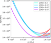 |
Fig. 1 Stellar lifetimes over the stellar masses of high-mass stars according to Yan et al. (2019, see their Fig. 3). The areas in which stellar lifetimes increase with initial stellar mass are marked in red. Instead of following these increases, the stellar lifetimes are kept constant beyond the minimum as shown on the colours of the different graphs. |
2.2 Computing the duration of SF
As shown in Wirth et al. (2021), the iron spread observed in GCs can be used to estimate the number of CCSNe that must have exploded before star formation ended. From this the time after which SF must have ended was computed assuming all stars with masses above 8 M⊙ explode as CCSNe. Since newer studies have shown that a large portion of massive stars end their life as a failed CCSN such an approach provides a lower limit for the duration of SF. The current paper aims to find an upper limit by investigating how long SF would have to last if only stars with masses below 20 M⊙ contribute to the iron enrichment. The value of 20 M⊙ is chosen, since according to O’Connor & Ott (2011) no failed CCSNe occur below this mass and according to Pejcha & Thompson (2015) and Sukhbold et al. (2016) the overwhelming majority of stars between 8 and 20 M⊙ explode as CCSNe.
The present work is based on Wirth et al. (2022), which uses an empirically gauged IMF as described originally in Marks et al. (2012) and updated by Yan et al. (2021). This IMF is a function of the initial gas cloud density and metallicity. Under the assumption that initially more massive stars have shorter lifetimes, the number of CCSNe required to explain the iron spread can be used to compute the duration of SF in GCs. The number of required CCSNe, NSN , computed from the iron spread, needs to be the result of an integral over the IMF, ξ(m), from an unknown minimum value, mlast , to the most massive star to explode with a mass of 20 M⊙ for the upper limit of the duration of SF (150 M⊙ is used for the lower limit of the duration of SF):
 (3)
(3)
 (4)
(4)
where α3 and k3 are the parameters of the IMF,  , for stellar initial masses, m, above 1 M⊙ . As mentioned above, these are functions of the metallicity and the density of the starforming gas cloud as given in Wirth et al. (2022).
The lifetime of a star with mass mlast then equals the time for which SF lasts. As in Wirth et al. (2022) the values from Fig. 3 in Yan et al. (2019), showing the life expectancy of a star over its initial mass, are used to compute the time at which SF ends from mlast . For details of the calculations the reader is referred to Wirth et al. (2022).
2.3 A program for detailed simulation
While a rough upper and lower estimate can be computed using the methods above, it is possible to do more accurate computations if concrete CCSN models are given. In this section, we therefore present the code SFDE that can compute SF durations from given tables for iron ejecta and the CCSN status (failed or exploded) depending on the stellar mass. This code computes the amount of iron to be produced as described above and then goes through the stars of the GC from the most massive to the least massive one. In Sect. 2.1, the assumption that each star ejects 0.074 M⊙ of iron upon explosion was mentioned. In SFDE the amount of iron ejected per star is given in an input file that allows the user to define initial stellar mass, m, dependent ejecta (information on input and output files are available in the README.md of SFDE). For each star that explodes the amount of iron is looked up from the table in the given input file and subtracted from the total amount of iron needed. If the amount of iron still required reaches 0, the last star contributing to SF was found. The life expectancy of this star equals the time for which SF lasts in the GC. An open source version of the code SFDE can be found on github1. For the present work version 1.0.0 is used.
3 Results
3.1 Changes to the computed initial masses
As explained in Sect. 2.1 two important changes were made to the algorithm computing the initial masses of GCs: metallicity dependent stellar remnant masses were added and β was computed using Eq. (2) instead of a linear function. Table A.1 shows both Mini computed in Wirth et al. (2022) and in this work next to each other. While the computed initial masses of most GCs are lower in this work, for some they did increase. As visible in Fig. 2, this change is uncorrelated to the metallicities, suggesting that the change in β is the dominant factor: Fig. 3 demonstrates the difference of β, when fitted linearly compared to the new power-law (Eq. (2)).
Figure 4 depicts the King concentration parameters and initial masses of our sample used in Wirth et al. (2022) and this work. It is visible that a larger concentration parameter automatically leads to a larger initial mass, which is to be expected since the other parameters W0 depends on, the pericentre radius and the SFE, do not change between this work and Wirth et al. (2022). Note that rh depends on Mini and is therefore not mentioned as a separate dependency of W0 . Note also that the largest W0 for the masses from Wirth et al. (2022) is slightly above the the point at which the linearly fitted β becomes negative. The reason why this still lead to a positive β in Wirth et al. (2022) is a bug, that lead to slightly smaller W0 being computed for the initial masses. In this plot we used the correctly computed W0 (see Wirth et al. 2022, for more details).
Figure 4 also shows that for W0 ≲ 7.0 the GCs becomes less compact (W0 decreases), while for W0 ≳ 7.0 the GCs becomes more compact (W0 increases) when comparing our upgraded method to the previous one. From Fig. 3, we learned that for 5.0 < W0 < 7.0, β(W0) is smaller in this paper than in Wirth et al. (2022), while it is the other way around for all other values of W0 . From Eq. (1) we learned that Tdiss is proportional to β and the mass-loss rate is, therefore, inversely proportional to β. For 5.0 < W0 < 7.0 (W0 > 7.0) the mass-loss rate of the GC is, therefore, decreased (increased) and therefore the computed initial mass is smaller (larger). The fact that W0 = 7.0 is not a hard boundary is due to the remnant masses now being metallic- ity dependent, while they were independent on the metallicity in Wirth et al. (2022).
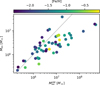 |
Fig. 2 New initial GC masses over the old ones colour-coded by metal- licity. The identity is shown in grey. |
3.2 The upper and lower limits for SF durations
Table A.1 shows measured and computed quantities for the 55 GCs from Bailin (2019). For Terzan 5 the SF durations could not be computed. Even if all CCSNe that it can produce happen (all stars with a mass above 8 M⊙ explode) the iron produced is insufficient to explain the iron abundance spread observed in this GC (see also Wirth et al. 2021, 2022). This suggests either that this GC, which is a bulge GC (Valenti et al. 2007) formed while being enriched externally or that the amount of gas expelled before forming the enriched population was significantly underestimated.
According to the data from Yan et al. (2019) a star with a mass of 20 M⊙ ends its life after ≈10.2 Myr. Therefore, no explosions should happen before this time and the respective values for tSF are expected to be larger than 10.2 Myr, which is the case. For most GCs the upper limit remains below 12 Myr. This is consistent with the findings of Bastian et al. (2013) who studied 130 young massive clusters with ages between 10 and 300 Myr observationally and found no ongoing SF within them, concluding that SF in GCs must have ended before the age of 10 Myr. This confirms the upper limit of our calculations. However, confirming the lower limit from observational studies is more difficult.
Observational studies on very young star clusters yield vastly different results for the duration of SF. Estimates for NGC 3603 YC for example go from 0.4 Myr (Kudryavtseva et al. 2012) to 10 Myr (Beccari et al. 2010). The density and velocity dispersion profiles of this cluster suggest a prompt monolithic collapse of a molecular cloud clump rather than a prolonged formation from merging sub-clusters (Banerjee & Kroupa 2015, 2018). For Westerlund 1 studies find 0.1 Myr (Kudryavtseva et al. 2012) to 1 Myr (Negueruela et al. 2010). Deshmukh et al. (2024) investigated the system of young clusters around M83 and found that for most of them the majority of the gas is cleared by pre-CCSN feedback. However, they also identify a massive (105.13M⊙) cluster that is still surrounded by gas and dust after 6.6 Myr. It should be pointed out here that these young clusters are more metal rich than the GCs studied in the present work, which means that the stars within them produce much stronger stellar winds (Dib et al. 2011). This leads to an earlier gas expulsion and, therefore, a shorter duration of SF.
The time after which SF ends for the different GCs is visualized in Fig. 5. As is visible the mass of the most massive star which explodes as a CCSN has a major impact on the time SF ends. Additionally, the spread between the GCs becomes larger for the cases with failed CCSNe compared to the cases where all stars above 8 M⊙ explode as a CCSNe. This is because the decrease in stellar life expectancies with mass is lower for high- mass O stars, than for low-mass O stars (see Fig. 3 in Yan et al. 2019).
The order in which GCs cease SF also changes. In Table A.1 we easily find pairs of GCs where one GC has a smaller duration of SF than the other if all stars are assumed to explode in CCSNe, but a larger duration of SF if only stars below 20 M⊙ are allowed to explode. This happens for example with NGC 5139 and NGC 5272 or NGC 6441 and NGC 6553. The cause of this is the differing IMFs for the individual GCs. A GC with a large Mini and low metallicity is expected to have a top-heavy IMF (Marks et al. 2012; Yan et al. 2021; Wirth et al. 2022).
How the IMF affects the SF duration is demonstrated in Fig. 6. This figure shows two IMFs for two fictional stellar clusters. For the blue cluster it is assumed that 4 CCSNe exploded before SF ends while for the orange one it is assumed to be only one. The coloured areas are the integral over all the stars that explode in a CCSN before SF ends that is they are equal to these numbers of CCSNe. Both cases, if the most massive CCSN progenitor has a mass of 150 M⊙ and if the most massive CCSN progenitor has a mass of 20 M⊙ , are shown. Note that the two blue (orange) areas both have an area of 4 (1). The low mass boundary of these areas then are equal to the masses of the last star to explode. The more massive this star is, the shorter is the duration of SF. It is therefore visible how the IMF shape and the assumptions about which stars explode in a CCSN both affect in which GC SF ceases first.
The duration of SF is especially important for the formation of multiple stellar populations in GCs, since a longer SF duration means a prolonged pollution of the star forming gas in the GC from stellar winds (Decressin et al. 2007; de Mink et al. 2009; Jecmen & Oey 2023). Additionally, binaries will also experience more encounters before SF ends if the duration of SF is long. This would lead to more binaries tightening and colliding, thus contributing their processed material to the surrounding gas (Sills & Glebbeek 2010; Wang et al. 2020; Dib et al. 2022; Kravtsov et al. 2022, 2024). It would also shorten the timescale for matter ejected from interacting binaries as discussed in Nguyen & Sills (2024). Their work investigates the evolution of binaries experiencing Roche-Lobe overflow. This leads to a spin-up of the secondary, which then due to its quick rotation cannot accrete more material, so that the polluted material is injected into the inter-stellar gas. However, they do not take dynamical interactions into account, therefore neglecting the effects of dynamical interactions and CCSNe. With dynamical interactions, we would expect the Roche-Lobe overflows to happen earlier, which means that material is ejected earlier and in a less polluted state. Therefore, an early SF period of up to ≈10 Myr has to be taken into account when investigating the formation of GCs and in rare cases (GCs with an unusually high amount of failed CCSNe) SF duration can last even longer, leading to an increased enrichment with light elements.
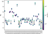 |
Fig. 4 Old and new values for W0 for the GCs in our sample. The values from Wirth et al. (2022) are shown using an empty circle, the values for this paper using a filled circle. Both are colour-coded for the initial masses of the clusters and connected with an arrow pointing in the direction of the new value computed in this work. |
 |
Fig. 5 Time after which SF ends depending on the initial cluster mass. The empty circles are for the case that all stars above 8 M⊙ explode in a CCSN, the filled circles show the upper limit for the SF duration, for which it is assumed that only stars with masses <20 M⊙ explode in CCSNe. The plot is colour-coded for the metallicity, [Fe/H]. |
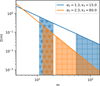 |
Fig. 6 Example of two IMFs (one shown in blue, one in orange) with different numbers of CCSNe. The number of CCSNe equals the integral from the least massive star to contribute to SF to the most massive star. The areas below the functions, therefore, show the number of CCSNe that are expected to explode before SF ends for the case that all stars up to a mass of 150 M⊙ explode in a CCSN (squares) and the case that only stars below 20 M⊙ explode (stars). In this work the mass of the least massive star to explode (lower boundary of the coloured areas) is computed from the known number of CCSNe and the known mass of the most massive star to explode. |
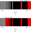 |
Fig. 7 Outcomes of stars depending on their stellar initial mass for NGC 288 and NGC 6366 using the CCSN model W18 of Sukhbold et al. (2016). Black shows mass ranges of failed CCSNe, red shows stars that explode as CCSNe and of which the iron is used in the formation of further stars and grey shows stars that explode as CCSNe after SF stopped. The time after which SF ends is marked by an arrow and written above the last star to explode. |
3.3 Precise calculations
To test the algorithm implemented in SFDE we use model W18 from Sukhbold et al. (2016). The reason we choose this model is that Sukhbold et al. (2016) provides precise values for the iron ejected by the CCSNe (see their Fig. 12). The SF duration computed using this model ( in Table A.1) is always larger than or equal to our lower limit (
 in Table A.1) and in most cases smaller than our upper limit (tSF in Table A.1). For NGC 6441 and NGC 6553 the iron produced by all CCSNe exploding in the GC is less than the amount of iron needed. Therefore, no SF duration could be computed for these GCs.
We also computed what happens if we assume that half of the residual gas is ejected from the cluster before iron enriched stars form ( in Table A.1). This effectively halves the amount of iron required to explain the iron spread, reducing the number of CCSNe required to produce the iron. For most GCs this significantly decreases the duration of SF. However, for GCs with already very small durations of SF it stays constant. This is caused by the low variations of stellar lifetimes in high-mass stars (no variation for the highest mass stars in this work).
Figure 7 is designed similar to the ‘barcodes’ shown in Fig. 13 of Sukhbold et al. (2016). The stars that contribute iron to the formation of new stars are marked in red. As is visible, a few of the stars with masses between 8 and 20 M⊙ still end in failed CCSNe and some of the stars with masses above 20 M⊙ explode as CCSNe. Additionally, since the estimates of ejecta masses from Sukhbold et al. (2016) are used, some stars produce a different amount from the 0.074 M⊙ assumed previously for computing the upper and lower limit.
To understand the influence these two effects have on the SF duration, the calculations for the two GCs that couldn’t produce enough iron in total (NGC 6441 and NGC 6553) were done again with the same mass ranges for failed CCSNe, but assuming that each CCSN produces 0.074 M⊙ of iron. The results are shown in Fig. 8, with blue used for the stars contributing to the iron spread to underline the difference in assumed masses of iron produced. Both NGC 6441 and NGC 6553 now have SF durations within the computed lower and upper limit, showing that the difference in iron output between the models has a significant effect on the SF duration. As Fig. 9 shows, even redoing the same calculations with Model W20 from Sukhbold et al. (2016), the most extreme model (when it comes to the ranges of failed CCSNe) available to us, still produces enough iron to explain the observed iron spread. However the SF duration now exceeds our previously computed upper limit. Therefore, the determination of the SF duration depends strongly on the precise iron ejecta of CCSN assumed for the calculation.
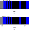 |
Fig. 8 Outcomes of stars depending on their initial stellar mass in NGC 6441 (a) and NGC 6553 (b) using the failed CCSNs of model W18 of Sukhbold et al. (2016), but a constant amount of 0.074 M⊙ of iron ejected per CCSN. Black shows mass ranges of failed CCSNe, blue shows stars that explode as CCSNe and of which the iron is used in the formation of further stars and grey shows stars that explode as CCSNe after SF stopped. The time after which SF ends is marked by an arrow and written above the last star to explode. |
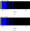 |
Fig. 9 Same as Fig. 8, but model W20 from Sukhbold et al. (2016) is used instead of W18. |
4 Discussion
4.1 Discussion of the assumptions
In this work, we improved the model from Wirth et al. (2022) by adding the effects of failed CCSNe and varying the amount of iron ejected per star. However, many aspects of this problem still require further investigation.
In our model, we assumed that all ejecta were preserved in the gas cloud and that the gas would be well mixed. As described in Calura et al. (2015) the ejecta from CCSNe cuts tunnels into the remaining gas cloud, through which gas can escape the GC easier. A loss of some of the CCSN ejecta would lead to a higher number of CCSNe required to produce the observed iron spread. On the other hand the CCSNe would produce pockets of higher metallicity, therefore, reducing the number of CCSN required. It is unclear, which of the two effects is dominant.
Furthermore, any kind of accretion and binary evolution is neglected. Both have been proposed as a possible cause for the multiple population phenomenon (de Mink et al. 2009; Sills & Glebbeek 2010; Gieles et al. 2018; Wang et al. 2020; Dib et al. 2022; Kravtsov et al. 2022, 2024; Nguyen & Sills 2024). Observational studies have shown that accretion onto a low-metallicity star can go on for up to 10 Myr (Fedele et al. 2010), which means that previously non-enriched stars may experience a small enrichment from polluted material entering the accretion disk. The magnitude of this effect is currently unknown. Additionally, stars do also show chemical enrichment, when ingesting a planet (Liu et al. 2024). These stars might become visible as exotic stars in a stellar cluster. In the current study both of these effects are neglected due to their unknown extent. Binary evolution would also greatly affect the outcomes of stellar evolution due to changes of the stellar mass caused by mass transfer and mergers. It is currently unclear what kind of ejecta are produced this way.
4.2 The current understanding of failed CCSNe
As mentioned in Sect. 1, it is not yet fully understood under which conditions massive stars explode as CCSNe and under which conditions they implode into a black hole (BH). Additionally, for those stars that do explode, the amount of iron ejected is not uniform. Portinari et al. (1998) describe the composition of CCSNe depending on the initial masses and metallicities of stars assuming all stars above 8 M⊙ explode. They find variations in iron outputs of about 3 orders of magnitude with a minimum iron output for stars with an initial mass of around 30 M⊙ .
Newer studies, however, describe the possibility of failed CCSNe. Additionally, if an explosion occurs, the nature of the remnant and, therefore, the ejecta is not only dependent on mass and metallicity. O’Connor & Ott (2011) point out that rotation significantly affects a CCSN due to centrifugal forces. Similarly Limongi & Chieffi (2018) found larger ejecta masses in fast rotating stars when compared to their slower or non-rotating counterparts. Sukhbold et al. (2016) point out the dependency on the structure of the pre-CCSN core, while Pejcha & Thompson (2015) find a strong dependency on the assumed required neutrino luminosity, showing how large the uncertainties are in current models of CCSNe. Finally, Ebinger et al. (2019) confirm the dependency on rotation and core structure and point out that the magnetic field of the star also affects the outcome of stellar evolution.
It is currently unknown how many stars and stars of which masses and metallicities actually end up exploding as a CCSN and what the exact amount and composition of the ejecta are. As was shown, this has a large effect on our results. To make more precise deductions about the duration of SF during GC formation, reliable CCSNe models for stars depending on metallicity, initial mass and rotation are needed. Furthermore, the initial distribution of stellar rotation in a just-born GC needs to be investigated.
5 Conclusions
This work revisits the results of Wirth et al. (2022) and studies the upper limit for the SF durations of GCs assuming that all stars more massive than 20 M⊙ result in failed CCSNe. The lower limit computed in Wirth et al. (2022) under the assumption that all stars above 8 M⊙ explode as CCSNe (≈3.5 Myr) and the upper limit computed here (≈10.5 Myr) differ by about a factor of 3 which has significant implications on the formation of GCs. It is also shown that failed CCSNe significantly affect the order in which GCs born simultaneously seize star formation. Because of this no conclusions about the duration of SF in different GCs relative to one another can be made without a more precise understanding of which CCSNe fail. However, as mentioned before, the longer durations of SF allow for longer periods of pollution from binaries and stellar winds to form multiple populations (de Mink et al. 2009; Sills & Glebbeek 2010; Gieles et al. 2018; Wang et al. 2020; Dib et al. 2022; Kravtsov et al. 2022, 2024; Nguyen & Sills 2024).
To further improve our understanding of the duration of SF, the nature of CCSN and the dependence of the amount of the ejected iron on stellar initial mass, metallicity and rotation needs to be investigated further. It is also important to develop a better understanding of the stellar rotation distribution in the young GCs as this largely influences the amount and chemical composition of ejecta produced (O’Connor & Ott 2011; Limongi & Chieffi 2018).
Acknowledgements
We thank an anonymous referee for many helpful suggestions. We also thank the DAAD-Eastern-European exchange programme at Bonn and Charles University for support.
Appendix A Additional table
The deduced masses, metallicities, numbers of CCSNe and times when SF ends for 55 Galactic GCs.
References
- Bailin, J. 2019, ApJS, 245, 5 [NASA ADS] [CrossRef] [Google Scholar]
- Banerjee, S., & Kroupa, P. 2015, MNRAS, 447, 728 [NASA ADS] [CrossRef] [Google Scholar]
- Banerjee, S., & Kroupa, P. 2018, Formation of Very Young Massive Clusters and Implications for Globular Clusters, 424, ed. S. Stahler, 143 [Google Scholar]
- Bastian, N., Cabrera-Ziri, I., Davies, B., & Larsen, S. S. 2013, MNRAS, 436, 2852 [NASA ADS] [CrossRef] [Google Scholar]
- Baumgardt, H., & Makino, J. 2003, MNRAS, 340, 227 [NASA ADS] [CrossRef] [Google Scholar]
- Beccari, G., Spezzi, L., De Marchi, G., et al. 2010, ApJ, 720, 1108 [NASA ADS] [CrossRef] [Google Scholar]
- Calura, F., Few, C. G., Romano, D., & D’Ercole, A. 2015, ApJ, 814, L14 [NASA ADS] [CrossRef] [Google Scholar]
- Decressin, T., Meynet, G., Charbonnel, C., Prantzos, N., & Ekström, S. 2007, A&A, 464, 1029 [NASA ADS] [CrossRef] [EDP Sciences] [Google Scholar]
- de Mink, S. E., Pols, O. R., Langer, N., & Izzard, R. G. 2009, A&A, 507, L1 [NASA ADS] [CrossRef] [EDP Sciences] [Google Scholar]
- Deshmukh, S., Linden, S. T., Calzetti, D., et al. 2024, The Clearing Timescale for Infrared-selected Star Clusters in M83 with HST [Google Scholar]
- Dib, S., Piau, L., Mohanty, S., & Braine, J. 2011, MNRAS, 415, 3439 [NASA ADS] [CrossRef] [Google Scholar]
- Dib, S., Gutkin, J., Brandner, W., & Basu, S. 2013, MNRAS, 436, 3727 [NASA ADS] [CrossRef] [Google Scholar]
- Dib, S., Kravtsov, V. V., Haghi, H., Zonoozi, A. H., & Belinchón, J. A. 2022, A&A, 664, A145 [NASA ADS] [CrossRef] [EDP Sciences] [Google Scholar]
- Ebinger, K., Curtis, S., Fröhlich, C., et al. 2019, ApJ, 870, 1 [NASA ADS] [Google Scholar]
- Fedele, D., van den Ancker, M. E., Henning, T., Jayawardhana, R., & Oliveira, J. M. 2010, A&A, 510, A72 [NASA ADS] [CrossRef] [EDP Sciences] [Google Scholar]
- Gieles, M., Charbonnel, C., Krause, M. G. H., et al. 2018, MNRAS, 478, 2461 [Google Scholar]
- Heger, A., Fryer, C. L., Woosley, S. E., Langer, N., & Hartmann, D. H. 2003, ApJ, 591, 288 [CrossRef] [Google Scholar]
- Hills, J. G. 1980, ApJ, 235, 986 [NASA ADS] [CrossRef] [Google Scholar]
- Jecmen, M. C., & Oey, M. S. 2023, ApJ, 958, 149 [NASA ADS] [CrossRef] [Google Scholar]
- Kravtsov, V., Dib, S., Calderón, F. A., & Belinchón, J. A. 2022, MNRAS, 512, 2936 [NASA ADS] [CrossRef] [Google Scholar]
- Kravtsov, V., Dib, S., & Calderón, F. A. 2024, MNRAS, 527, 7005 [Google Scholar]
- Kroupa, P., Aarseth, S., & Hurley, J. 2001, MNRAS, 321, 699 [NASA ADS] [CrossRef] [Google Scholar]
- Kudryavtseva, N., Brandner, W., Gennaro, M., et al. 2012, ApJ, 750, L44 [NASA ADS] [CrossRef] [Google Scholar]
- Lada, C. J., Margulis, M., & Dearborn, D. 1984, ApJ, 285, 141 [NASA ADS] [CrossRef] [Google Scholar]
- Limongi, M., & Chieffi, A. 2018, ApJS, 237, 13 [NASA ADS] [CrossRef] [Google Scholar]
- Liu, F., Ting, Y.-S., Yong, D., et al. 2024, Nature, 627, 501 [NASA ADS] [CrossRef] [Google Scholar]
- Maoz, D., & Graur, O. 2017, ApJ, 848, 25 [Google Scholar]
- Marino, A. F., Milone, A. P., Karakas, A. I., et al. 2015, MNRAS, 450, 815 [NASA ADS] [CrossRef] [Google Scholar]
- Marino, A. F., Yong, D., Milone, A. P., et al. 2018, ApJ, 859, 81 [NASA ADS] [CrossRef] [Google Scholar]
- Marino, A. F., Milone, A. P., Renzini, A., et al. 2019, MNRAS, 487, 3815 [CrossRef] [Google Scholar]
- Marks, M., Kroupa, P., Dabringhausen, J., & Pawlowski, M. S. 2012, MNRAS, 422, 2246 [NASA ADS] [CrossRef] [Google Scholar]
- Milone, A. P. 2015, MNRAS, 446, 1672 [NASA ADS] [CrossRef] [Google Scholar]
- Milone, A. P. 2016, Mem. Soc. Astron. Italiana, 87, 303 [NASA ADS] [Google Scholar]
- Milone, A. P., Bedin, L. R., Piotto, G., et al. 2015a, MNRAS, 450, 3750 [CrossRef] [Google Scholar]
- Milone, A. P., Marino, A. F., Piotto, G., et al. 2015b, ApJ, 808, 51 [NASA ADS] [CrossRef] [Google Scholar]
- Milone, A. P., Piotto, G., Renzini, A., et al. 2017, MNRAS, 464, 3636 [Google Scholar]
- Negueruela, I., Clark, J. S., & Ritchie, B. W. 2010, A&A, 516, A78 [NASA ADS] [CrossRef] [EDP Sciences] [Google Scholar]
- Nguyen, M., & Sills, A. 2024, ApJ, 969, 18 [NASA ADS] [CrossRef] [Google Scholar]
- O’Connor, E., & Ott, C. D. 2011, ApJ, 730, 70 [Google Scholar]
- Pascale, M., Dai, L., McKee, C. F., & Tsang, B. T. H. 2023, ApJ, 957, 77 [NASA ADS] [CrossRef] [Google Scholar]
- Pejcha, O. 2020, in Reviews in Frontiers of Modern Astrophysics; From Space Debris to Cosmology, 189 [CrossRef] [Google Scholar]
- Pejcha, O., & Thompson, T. A. 2015, ApJ, 801, 90 [NASA ADS] [CrossRef] [Google Scholar]
- Portinari, L., Chiosi, C., & Bressan, A. 1998, A&A, 334, 505 [NASA ADS] [Google Scholar]
- Sills, A., & Glebbeek, E. 2010, MNRAS, 407, 277 [NASA ADS] [CrossRef] [Google Scholar]
- Sukhbold, T., Ertl, T., Woosley, S. E., Brown, J. M., & Janka, H. T. 2016, ApJ, 821, 38 [NASA ADS] [CrossRef] [Google Scholar]
- Valenti, E., Ferraro, F. R., & Origlia, L. 2007, AJ, 133, 1287 [Google Scholar]
- Wang, L., Kroupa, P., Takahashi, K., & Jerabkova, T. 2020, MNRAS, 491, 440 [Google Scholar]
- Wirth, H., Jerabkova, T., Yan, Z., et al. 2021, MNRAS, 506, 4131 [NASA ADS] [CrossRef] [Google Scholar]
- Wirth, H., Kroupa, P., Haas, J., et al. 2022, MNRAS, 516, 3342 [NASA ADS] [CrossRef] [Google Scholar]
- Yan, Z., Jerabkova, T., Kroupa, P., & Vazdekis, A. 2019, A&A, 629, A93 [NASA ADS] [CrossRef] [EDP Sciences] [Google Scholar]
- Yan, Z., Jerábková, T., & Kroupa, P. 2021, A&A, 655, A19 [NASA ADS] [CrossRef] [EDP Sciences] [Google Scholar]
All Tables
The deduced masses, metallicities, numbers of CCSNe and times when SF ends for 55 Galactic GCs.
All Figures
|
Fig. 1 Stellar lifetimes over the stellar masses of high-mass stars according to Yan et al. (2019, see their Fig. 3). The areas in which stellar lifetimes increase with initial stellar mass are marked in red. Instead of following these increases, the stellar lifetimes are kept constant beyond the minimum as shown on the colours of the different graphs. |
| In the text | |
|
Fig. 2 New initial GC masses over the old ones colour-coded by metal- licity. The identity is shown in grey. |
| In the text | |
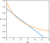 |
Fig. 3 β(W0) fitted linearly (blue) and as a power-law (orange, Eq. (2)). |
| In the text | |
|
Fig. 4 Old and new values for W0 for the GCs in our sample. The values from Wirth et al. (2022) are shown using an empty circle, the values for this paper using a filled circle. Both are colour-coded for the initial masses of the clusters and connected with an arrow pointing in the direction of the new value computed in this work. |
| In the text | |
|
Fig. 5 Time after which SF ends depending on the initial cluster mass. The empty circles are for the case that all stars above 8 M⊙ explode in a CCSN, the filled circles show the upper limit for the SF duration, for which it is assumed that only stars with masses <20 M⊙ explode in CCSNe. The plot is colour-coded for the metallicity, [Fe/H]. |
| In the text | |
|
Fig. 6 Example of two IMFs (one shown in blue, one in orange) with different numbers of CCSNe. The number of CCSNe equals the integral from the least massive star to contribute to SF to the most massive star. The areas below the functions, therefore, show the number of CCSNe that are expected to explode before SF ends for the case that all stars up to a mass of 150 M⊙ explode in a CCSN (squares) and the case that only stars below 20 M⊙ explode (stars). In this work the mass of the least massive star to explode (lower boundary of the coloured areas) is computed from the known number of CCSNe and the known mass of the most massive star to explode. |
| In the text | |
|
Fig. 7 Outcomes of stars depending on their stellar initial mass for NGC 288 and NGC 6366 using the CCSN model W18 of Sukhbold et al. (2016). Black shows mass ranges of failed CCSNe, red shows stars that explode as CCSNe and of which the iron is used in the formation of further stars and grey shows stars that explode as CCSNe after SF stopped. The time after which SF ends is marked by an arrow and written above the last star to explode. |
| In the text | |
|
Fig. 8 Outcomes of stars depending on their initial stellar mass in NGC 6441 (a) and NGC 6553 (b) using the failed CCSNs of model W18 of Sukhbold et al. (2016), but a constant amount of 0.074 M⊙ of iron ejected per CCSN. Black shows mass ranges of failed CCSNe, blue shows stars that explode as CCSNe and of which the iron is used in the formation of further stars and grey shows stars that explode as CCSNe after SF stopped. The time after which SF ends is marked by an arrow and written above the last star to explode. |
| In the text | |
|
Fig. 9 Same as Fig. 8, but model W20 from Sukhbold et al. (2016) is used instead of W18. |
| In the text | |
Current usage metrics show cumulative count of Article Views (full-text article views including HTML views, PDF and ePub downloads, according to the available data) and Abstracts Views on Vision4Press platform.
Data correspond to usage on the plateform after 2015. The current usage metrics is available 48-96 hours after online publication and is updated daily on week days.
Initial download of the metrics may take a while.