| Issue |
A&A
Volume 698, June 2025
|
|
|---|---|---|
| Article Number | A203 | |
| Number of page(s) | 12 | |
| Section | Extragalactic astronomy | |
| DOI | https://doi.org/10.1051/0004-6361/202451959 | |
| Published online | 23 June 2025 | |
Unraveling the Lyman continuum emission of Ion3: Insights from HST multiband imaging and X-Shooter spectroscopy
1
Dipartimento di Fisica, Università degli Studi di Milano, Via Celoria 16, I-20133 Milano, Italy
2
INAF – OAS, Osservatorio di Astrofisica e Scienza dello Spazio di Bologna, via Gobetti 93/3, I-40129 Bologna, Italy
3
Space Telescope Science Institute, 3700 San Martin Drive, Baltimore, MD 21218, USA
4
Department of Physics and Astronomy, Johns Hopkins University, Baltimore, MD 21218, USA
5
INAF – IASF Milano, Via A. Corti 12, I-20133 Milano, Italy
6
Department of Astronomy, University of Massachusetts Amherst, Amherst, MA 01002, USA
7
INAF – Osservatorio Astronomico di Roma, via di Frascati 33, 00078 Monte Porzio Catone, Italy
8
Istituto Nazionale di Astrofisica – Osservatorio Astronomico di Trieste, Via Tiepolo 11, Trieste, Italy
9
IFPU – Institute for Fundamental Physics of the Universe, Via Beirut 2, 34014 Trieste, Italy
10
Istituto Nazionale di Astrofisica, Vicolo dell’Osservatorio 5, 35137 Padova, Italy
11
Università di Salerno, Dipartimento di Fisica “E.R. Caianiello”, Via Giovanni Paolo II, 132, I-84084 Fisciano (SA), Italy
12
INAF – Osservatorio Astronomico di Capodimonte, Via Moiariello 16, I-80131 Napoli, Italy
13
INFN – Gruppo Collegato di Salerno – Sezione di Napoli, Dipartimento di Fisica “E.R. Caianiello”, Università di Salerno, via Giovanni Paolo II, 132, I-84084 Fisciano (SA), Italy
14
Dipartimento di Fisica e Scienze della Terra, Università degli Studi di Ferrara, via Saragat 1, I-44122 Ferrara, Italy
15
Kapteyn Astronomical Institute, University of Groningen, P.O. Box 800 9700AV Groningen, The Netherlands
16
Cosmic Dawn Center (DAWN), Copenhagen, Denmark
⋆ Corresponding author.
Received:
22
August
2024
Accepted:
21
April
2025
Abstract
We provide a comprehensive analysis of Ion3, the most distant LyC leaker at z = 3.999, using multiband HST photometry (F390W, F814W, and F140W) and reevaluated X-Shooter spectroscopy. Deep HST F390W imaging enables us to probe uncontaminated LyC flux blueward of ∼880 Å. In this work, the nonionizing UV 1500 Å/2800 Å flux was probed with the F814W/F140W band. High angular resolution allowed us to properly mask low-z interlopers and prevent contamination of measured LyC radiation. We confirm the detection of LyC flux at a signal-to-noise ratio of S/N ∼ 3.5 and estimate the escape fraction of ionizing photons to be in the range fesc, rel = 0.06–1, depending on the adopted IGM attenuation. A morphological analysis of Ion3 reveals a clumpy structure made up of two main components, Ion3A and Ion3B, with effective radii of Reff ∼ 180 pc and Reff < 100 pc, respectively, along with a total estimated delensed area in the rest-frame 1600 Å of 4.2 kpc2. We confirm the presence of faint ultraviolet spectral features, including HeIIλ1640, CIII]λ1907,1909, and [NeIII]λ3968, with a rest-frame equivalent width EW(HeII) =(1.6 ± 0.7) Å and EW(CIII]) =(6.5 ± 3) Å. From the [OII]λλ3726,3729 and [CIII]λ1909/CIII]λ1906 doublets, we derived electron densities of ne[OII] = 2300 ± 1900 cm−3 and ne[CIII] > 104 cm−3, corresponding to an interstellar medium (ISM) pressure log(P/k) > 7.90. Furthermore, we derived an intrinsic SFR(Hα) ≈77 M⊙ yr−1 (corresponding to ΣSFR = 20 M⊙ yr−1 kpc−2 for the entire galaxy) and subsolar metallicity 12 + log(O/H) = 8.02 ± 0.20 using the EW(CIII]) as a diagnostic. The detection of [NeIII]λ3968 line and [OII]λλ3726,3729 offer an estimate of the ratio [OIII]λ5007/[OII]λλ3727,29 of O32 > 50 and a high ionization parameter, log U > −1.5, using empirical and theoretical correlations. These measurements imply remarkably high ionization levels and density conditions produced by an ongoing bursty star formation, observed during an ionizing, optically thin phase of the ISM along the line of sight.
Key words: galaxies: evolution / galaxies: formation / galaxies: general / galaxies: high-redshift
Deceased.
© The Authors 2025
 Open Access article, published by EDP Sciences, under the terms of the Creative Commons Attribution License (https://creativecommons.org/licenses/by/4.0), which permits unrestricted use, distribution, and reproduction in any medium, provided the original work is properly cited.
This article is published in open access under the Subscribe to Open model. This email address is being protected from spambots. You need JavaScript enabled to view it. to support open access publication.
1. Introduction
Directly detecting Lyman continuum radiation (LyC, λ < 912 Å) emitted by star-forming galaxies at redshifts of 3 < z < 4.5 is a challenging task. After more than 20 years of searching for LyC-emitting galaxies using different approaches, such as spectroscopy and broad- and narrowband photometry, only a handful of LyC sources have been confirmed at these redshifts (e.g., Vanzella et al. 2016, 2018; Shapley et al. 2016; Steidel et al. 2018; Fletcher et al. 2019; Marques-Chaves et al. 2021, 2022; Rivera-Thorsen et al. 2019). The current number of galaxies at these redshifts with confirmed LyC detection is not sufficient to build the robust and statistically significant sample required to characterize the properties of LyC-leaking galaxies and understand the mechanisms and conditions that control the LyC emissivity. Several factors limit our ability to successfully detect hydrogen-ionizing radiation emitted by star-forming galaxies. First, LyC radiation is produced by O-type and other massive, short-lived stars and is easily absorbed by neutral hydrogen and dust in the interstellar medium (ISM). This absorption makes it difficult for LyC radiation to be observable and the situation is further exacerbated by the increasing intervening opacity of the circumgalactic and intergalactic medium (CGM and IGM) with increasing redshift (Worseck et al. 2014). Second, LyC flux can easily be contaminated by low-redshift sources, which further complicates the task of ascertaining the nature of suspected LyC emission without high-angular resolution, multiband imaging (e.g., Vanzella et al. 2010; Nestor et al. 2011). Overcoming these challenges and accurately measuring the escape fraction (fesc) of LyC radiation from galaxies is crucial for understanding how the Epoch of Reionization (EoR) progressed, as well as for investigating the formation and evolution of galaxies.
In recent years, faint, low-mass galaxies have been suggested as the most likely main contributors to the global budget of ionizing photons (e.g., Finkelstein et al. 2019; Simmonds et al. 2024). The relative contribution of high-mass galaxies, however, still remains to be quantified, and these sources still remain potential important candidates of substantial LyC emission (e.g., Naidu et al. 2020). Due to the high IGM opacity beyond z ∼ 4.5 (Inoue & Iwata 2008; Inoue et al. 2014), it is impossible to directly probe the ionizing UV radiation from galaxies at the EoR. For these reasons, there are ongoing efforts to identify and study large samples of LyC emitters at low redshift (e.g., Flury et al. 2022; Jaskot et al. 2024a) that plausibly are good proxies (or “analogs”) of z > 6 galaxies to inform on how to best trace LyC leakers at the EoR by means of robustly calibrated indirect diagnostics. Results from Lyman alpha (Lyα) radiation transfer models suggest that a promising LyC tracer is a multiply peaked Lyα emission line (e.g., Verhamme et al. 2015; Behrens et al. 2014). Correlations between the LyC emissivity and the Lyα spectral properties have been investigated using samples of low-z and high-z LyC-leaking galaxies and these studies have shown that a multipeaked Lyα profile with a narrow emission peak close to the systemic redshift would indicate an optically thin medium to LyC radiation (e.g., Verhamme et al. 2017; Izotov et al. 2018, 2021a; Vanzella et al. 2020; Rivera-Thorsen et al. 2017). Furthermore, Naidu et al. (2022) demonstrated that the properties of the Lyα line as velocity separation between Lyα peaks (Vsep) and the central escape fraction of Lyα can discriminate between sources with high and low escape fractions of LyC photons. Nevertheless, it has been recognized that describing correlations between the LyC emissivity and other properties of the galaxies is a multiparameter problem; thus, to indirectly identify likely LyC leakers and predict their escape fraction, different physical properties need to be considered simultaneously and described in terms of multiply varied distribution functions. For example, the results from a multivariate analysis by Jaskot et al. (2024a) suggested that the EW of Lyman absorption features and the UV β slope are the most important parameters, followed by escape fraction of Lyα photons (fesc,Lyα), dust excess (E(B–V)neb), star formation rate surface density (ΣSFR), and the O32 index. These conclusions are based on a sample of 35 local (z ∼ 0.3) LyC leakers (e.g., LzLCS, Flury et al. 2022). A similar set of indirect tracers of LyC has also been studied for sources at high redshift (z ∼ 3 − 4), however, larger samples of LyC leakers are required to better constrain the multivariate models that robustly predict fesc. Currently, the most effective diagnostics to predict fesc of z ∼ 3 sources adopt dust attenuation, the UV β slope, the O32 index, and ΣSFR as the best physical parameters (Jaskot et al. 2024b).
This work presents results from new HST multiband imaging of Ion3 (PI: Meštrić, ID 17133) which, at a redshift of z = 3.999, is the most distant confirmed LyC leaker to date (Vanzella et al. 2018). Ion3 shows strong LyC leakage and quadruple-peaked Lyα emission features, with a peak located at the resonance frequency, and a very blue ultraviolet continuum slope (β slope) of −2.5 ± 0.25. The photometric SED from VLT/HAWKI Ks and Spitzer/IRAC 3.6 μm and 4.5 μm bands (available from the Hubble frontier fields project, Lotz et al. 2017) reveals a clear excess in the 3.6 μm channels ascribed to prominent Hα line emission (with a rest-frame EW of ∼1000 Å). From the same data, a stellar mass of ∼ 1.5 × 10⁹ M⊙, a SFR of ≃140 M⊙ yr−1 and a young age of ∼10 Myr have been inferred (Vanzella et al. 2018).
The depth and high-angular resolution, combined with the wavelength coverage of HST imaging, allowed us to measure the fesc and successfully check for and remove potential contamination by a low-z interloper. Furthermore, we combined HST imaging with archival spectroscopy (FORS2 and X-Shooter) and Spitzer/IRAC 3.6 μm data to investigate the ISM conditions and mechanisms behind LyC leakage in Ion3 in depth. This work is organized as follows. In Sect. 2, we describe our HST data reduction procedure. In Sect. 3, we detail the morphological, photometric, and spectroscopic analyses. In Sect. 4, we define and evaluate the escape fraction of ionizing photons. Section 5 presents our results and discussion. Lastly, in Sect. 6, we summarize our work and give our conclusions. Throughout this work, we adopt a Λ-CDM cosmology, with H0 = 68 km s−1 Mpc−1, Ωm = 0.3, and ΩΛ = 0.7.
2. Data
2.1. HST data
The HST data used in this work consist of three bands of imaging using both the UV/optical and near-infrared (NIR) channels of the Wide Field Camera 3 (WFC3, Marinelli & Dressel 2024), namely, F390W, F814W and F140W. We used a long exposure time in F390W (25 540 s across nine exposures and three visits) to detect LyC radiation, from 890 Å and blueward, from Ion 3. Shorter exposures were used to measure the non-ionizing UV flux at λ ∼ 1400 Å to ∼1950 Å) and stellar continuum morphology (8030 s in F814W) as well as to improve the SED modeling to measure properties, such as the stellar mass, and to check for low-z interlopers (13 900 s in F140W). The full width half maximum (FWHM) of the point spread functions (PSFs) for the F390W and F8140W filters are very similar: 0.070″ and 0.074″, respectively. Therefore, a PSF size matching was not performed between these two bands. Despite an expected FWHM of ∼0.141″, which is notably different from other two observed bands, the PSF-matching to the F140W filter was not performed because this filter was only used for contamination checks in our analysis.
We applied a custom data reduction pipeline to this data, utilizing routines from the Drizzlepac software (Gonzaga et al. 2012; Hoffmann et al. 2021), as well as LACOSMIC (van Dokkum 2001) and custom routines similar to those used in several previous studies with WFC3 imaging (e.g., Prichard et al. 2022; Revalski et al. 2023; Wang et al. 2024). We first prepared the individual exposures using CALWF3, which produces the initial dark and flat-field corrections, debiasing, sink pixel rejection, and post-flash subtraction. Firstly, we flagged hot pixels using a variable threshold. The number of hot pixels varies as a function of location on the detector when using a constant threshold, due to imperfections in the corrections made to account for charge transfer efficiency (CTE) degradation. By fitting the number of hot pixels as a function of row number, we can then adjust the detection threshold, so that the hot pixels were evenly distributed (Prichard et al. 2022). Next, after masking out sources detected in each image, we estimated the background levels in the two chips, which were then equalized to remove any offsets between the amplifiers.
We then proceeded to remove cosmic rays from the exposures. ASTRODRIZZLE was used for an initial run to detect cosmic rays. Read-out cosmic rays (ROCRs) were removed by flagging pixels within five pixels of these detected cosmic rays that are more than 2.75σ below the background level. Afterwards, we used LACOSMIC to remove the remaining cosmic rays from each frame. Finally, we used the UPDATEWCS routine to reset the astrometry of each exposure to that obtained from the Hubble guide stars, which are tied to the GAIA astrometry.
Finally, we aligned the cleaned exposures onto the same WCS grid and combined them using routines from Drizzlepac. We used the TWEAKREG routine to match the positions of bright, compact sources across the image, and the ASTRODRIZZLE routine to combine exposures into our final science images. We first created “unaligned” drizzles by adding the exposures from each visit together. This results in one image in the F814W and F140W bands and three F390W images. Using TWEAKREG, we matched compact sources in each exposure to their counterparts in the unaligned image and adjusted the wcs of the exposures to align with the drizzle. We then re-combined the aligned exposures to produce final visit-level drizzles.
We attempted to match these visit-level drizzles to the GAIA catalog (Gaia Collaboration 2023), but there were too few unsaturated stars in our field whose centroids could be accurately measured. Therefore, we used TWEAKREG to align our images instead. For the F390W data, we measured the “tweak” required to align the three visit-level drizzles to each other, applied that tweak to the exposures making up each visit, and combined these aligned exposures into a final F390W image. Finally, we applied the same procedure to align the F814W and F140W images with the F390W: measuring the required shift to align the drizzles to the F390W image, applying it to the individual exposures, and then drizzling these into the final science images.
This ensures excellent relative astrometry despite some uncertainty in the absolute astrometry. Each time an image was “tweaked” to align with another, the spread of the differences between the locations of the matched sources gives an indication of the uncertainty in the shift. We find that the F390W exposures are aligned to each other to an accuracy of ≈2 mas (0.05 native pixel), the F814W image is aligned to the F390W to within 10 mas (0.25 native pixel), and the F140W matches the F390W to within 13 mas (0.04 native pixel).
2.2. VLT X-Shooter data
The four-hour X-Shooter observations Ion3 were carried out in November 2017 with an average seeing conditions of 0.8 arcsec (prog. 098.A-0665, P.I. Vanzella), providing a final spectrum spanning the range 3400 Å–24 000 Å, with spectral resolution of 35 − 60 km s−1. The data were partially presented by Vanzella et al. (2018), focusing mainly on the Lyα line and possible detection of [OII]λλ3726,3729 used to measure systemic redshift. In this work, we carefully analyze the full spectral range reporting on additional emission ultraviolet features tracing the physical properties of the interstellar medium and the ionizing source. We refer to Vanzella et al. (2018, and references therein) for details on the X-Shooter data reduction.
3. Analysis
Our main scientific goals are threefold: (1) evaluate the escape fraction of ionizing photons, while eliminating possible low-z contaminants, (2) investigate the morphology of the system and, (3) study the ISM properties of the LyC-emitting regions. The main results presented in this section are summarized in Table 1.
Resulting photometry, spectroscopy, and physical properties of Ion3.
3.1. Lyman continuum emission and morphological analysis
Figure 1 shows the LyC image at the redshift of Ion3 and the non-ionizing radiation at λ ∼ 1600 Å and at λ ∼ 2800 Å, from the F390W, F814W, and F140W bands, respectively. F814W data are much shallower than those in F390W (having 5σ magnitude limits maglim(F814W) ∼ 25.41 and maglim(F390W) ∼ 28.20, respectively). We report the detection of a source, designated D in Fig. 1, located 0.6 arcsec from Ion3. Source D shows magnitudes of 28.00 ± 0.15 and 27.50 ± 0.08 in the F390W and F140W filters, respectively, but is not detected in F814W. We suspect that source D is a lower-redshift contaminant, previously unknown until this Hubble imaging analysis. Although we lacked a redshift confirmation for source D, now it is clear that LyC signal detected from the ground-based FORS spectroscopic data presented in Vanzella et al. (2018) is probably contaminated by source D flux, which leaks into the slit. The deep F390W image probing LyC shows three tentative clumps at the location of Ion3 (A, B, and C), two of which (A and B) resemble the geometry of the double-blob morphology of Ion3 observed in the F814W image. Given the shallower F814W image, the non-detection of the object C does not necessarily rule out its LyC nature. However, we conservatively mask the source C in the following statistical analysis.
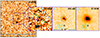 |
Fig. 1. Left: HST F390W band thumbnail image of Ion3, size 5″ × 5″. Three zoom-in cut outs of sizes 1.5″ × 1.5″ are shown on the right side and F390W, F814W, and F140W bands with their expected PSFs in the upper left corner, blue circle. The HST F390W band probes LyC flux from 890 Å and blueward (note: the F390W band misses the first ∼20 Å of LyC flux). Green arrows point toward two clumpy structures (A and B) at z = 3.999 where LyC flux is detected. The third clumpy structure, pointed to with a purple arrow (C), very close to the LyC leaking sources, is most likely a low-z interloper, which is masked before the LyC flux is measured. Finally, the blue circle is adopted as the aperture to measure LyC flux, with a diameter of 0.36″, while the cyan rectangle (D) encloses the source that probably contaminates the LyC flux detected from the FORS spectroscopy. The blue lines indicate the VLT FORS slit position, showing that source D enters the slit and likely contaminates the LyC flux detected in FORS spectroscopy. The grey lines show the VLT X-Shooter slit position. The second observed band is F814W and covers non-ionizing UV flux, where both LyC leaking clumps are detected. The third panel is the F140W band, where Ion3 is detected as a single bright blob, which is not resolved due to the lower spatial resolution of WFC3/IR. The three small green diamonds are centered on the clumpy sources A, B, and C in the F390W image, with their corresponding positions also shown in the F814W and F140W images. It is noticeable that clump A detected in F390W is slightly offset from clump A observed in F814W. |
We perform photometric measurements using the Astropy package and the photometry of astronomical sources with Photutils (Bradley et al. 2024). The center of the aperture was defined by inspecting all three HST bands, and was placed between the detected clumps A and B; to check the robustness of our measurements, we moved the aperture center a two pixels around the selected center and concluded that the resulting photometry was unaffected. Before measuring the LyC flux in F390W, we first mask the source C and construct a photometric curve of growth (CoG) with a series of apertures centered on the source. The CoG is computed by summing the flux in a predefined series of apertures to determine the optimal diameter for flux measurement (the peak at which the CoG reaches its maximum before entering the noise regime), which in our case is 12 pixels or 0.36″ in diameter (blue circle, Fig. 1). This aperture includes both A and B peaks in F390W as well as most of the F814W flux. The mean-background local sky level was measured within an annulus aperture (rin = 7 pix and rout = 9 pix). The evaluated LyC flux and magnitude of Ion3 measured in the F390W band are Fν = 1.07 ± 0.3 × 10⁻³¹ erg/cm2/s/Hz or mF390W = 28.8 ± 0.3, with a signal-to-noise ratio of S/N = 3.5.
To confirm the reliability and robustness of the measured LyC flux, we determined the background level in the parts of the images surrounding Ion3. As a first step, we create 5″ × 5″ thumbnails centered on Ion3 in all three observed HST bands. Since our aim is to probe the background around Ion3 in the F390W band, we detect all sources in F814W and F140W, adopting a detection threshold of 5σ. In the second step, all positions of detected sources in F814W and F140W are masked (in total 3 sources) in the F390W image to reduce contamination. Finally, we probe the background by randomly placing 10 000 overlapping apertures, of the same size used to measure the reported flux (0.36″ in diameter), over the 5″ × 5″ F390W thumbnail image. The resulting background flux measurements are presented in the histogram density plot (Fig. 2); we confirm that the emission observed at the location of Ion3 is significant, at 3.5σ level. Finally, the magnitude errors were evaluated by adopting the standard expression mag_error = 1.086 × err_flux /flux, where the term err_flux is the standard deviation derived from 10 000 background apertures, and flux is the measured flux from Ion3 within the defined aperture. The same approach was applied for magnitude measurement in F814W band whose resulting magnitude is mF814W = 24.20 ± 0.07.
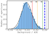 |
Fig. 2. Histogram density plot of randomly placed 10 000 apertures over a 5″ × 5″ F390W image centered on Ion3. The black line is the Gaussian fit to the measured fluxes (in ADU) from 10 k apertures, with a resulting mean value of 0.001 and a 1σ of 0.0119, marked with a red dashed line (2σ and 3σ are marked with yellow and green dashed lines, respectively). The thick blue dashed line represents the background-subtracted, clean, non-contaminated LyC signal of Ion3, while thin gray dashed line is measured non-contaminated LyC signal before the background subtraction. |
To measure the effective radius of both clumps, we applied the method described in Meštrić et al. (2022). The two-dimensional (2D) modeling of the clump light profiles was performed using GALFIT (Peng et al. 2002, 2010), resulting in estimated physical sizes for both components (Ion3A and Ion3B). The sizes were derived from HST F814W imaging (probing UV rest-frame flux) after fixing the Sérsic index to 0.5 and leaving magnitude and half-light radii as free parameters. The resulting effective radii are Reff ∼ 180 ± 90 pc for Ion3A and an upper limit of Reff < 100 pc for Ion3B. The estimated sizes for both clumps were corrected for a total magnification of μtot = 1.3 (Caminha et al. 2016). The GALFIT model and residuals are shown in Fig. 3.
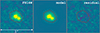 |
Fig. 3. Results from Galfit modeling. The first panel shows the original F814W image of Ion3 covering the non-ionizing UV flux with 2σ contour in red, also overlaid in other two panels. The second panel is the resulting model from Galfit and the third panel is a residual map. |
3.2. X-Shooter spectroscopy
Our X-Shooter data includes a total of four hours of exposure time, divided into four observation blocks (OBs); the spectral range covered is 3000–5595 Å (600–1119 Å rest frame) by the UVB arm, 5595–10 240 Å (1119–2048 Å rest frame) by the VIS arm, and 10 240–24 800 Å (2048–4960 Å rest frame) by the NIR arm. We chose to focus our analysis mostly on the spectra from the VIS and NIR arms, since the wavelength coverage of the UVB arm has been observed with deeper FORS spectroscopy, as reported in Vanzella et al. (2018). We combine the 4 OBs by creating an average weighted 2D stacked spectrum using the IRAFIMCOMBINE task (both for the VIS and NIR data).
3.2.1. X-Shooter VIS-arm
In order to increase the S/N of the VIS spectrum, we binned the 2D spectrum (whose initial resolution element is 0.2 Å/pix) by a factor of 9 in the dispersion direction using the IRAFBLKAVG task. This produced a binned 2D spectrum with a 1.8 Å/pix resolution element. Subsequently, the 1D spectrum was extracted within a window of 1.6 arcsec centered on the spatial position of Ion3 in the slit, traced by its continuum. The result is shown in Fig. 4. After a careful inspection of the 1D and 2D X-Shooter VIS binned spectra, in addition to Lyα, NVλλ1238,1242, [CII]λ1335.71, and CIVλ1550 lines (Vanzella et al. 2018), we detected HeIIλ1640 and CIII]λλ1907,1909 features. Before measuring the flux and EW of newly detected emission lines, we fit the continuum and subtract the resulting fit from the original spectrum, creating a continuum-subtracted spectrum. The continuum fitting was done using the IRAF task CONTINUUM, where we used a second-order polynomial, avoiding parts of the spectrum where prominent emission and absorption features are expected. The flux and equivalent width (EW) of detected emission lines are evaluated by fitting a Gaussian function to the observed spectral features. This fitting procedure utilizes the LevMarLSQFitter class from the astropy library (unless otherwise noted). Uncertainties associated with the measured flux and EW are propagated from the covariance matrix output by the fitting algorithm. This matrix provides information on both the uncertainties and the correlations between the fitted parameters. The resulting fluxes and EWs are  , EW(HeII) = 1.6 ± 0.7 Å and FCIII] = 1.12 ± 0.49 × 10⁻¹⁷ erg/s/cm2, EW(CIII]) = 6.5 ± 3 Å. The fitted emission features and their corresponding 1D, 2D, and 3D spectrograms are shown in Fig. 5.
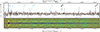 |
Fig. 4. X-Shooter VIS-arm 1D spectra (upper panel) and 2D spectra (bottom panel) covering the rest-UV wavelengths from ∼1180 Å–1940 Å. The spectrum (black) is binned by a factor of 9 to increase the S/N of the continuum and other spectroscopic features, while 1σ uncertainty is presented in red color and orange line shows 0 flux level. The displayed 1D spectrum is continuum subtracted. The location of the reported and analyzed emission features (HeIIλ1640 and CIII]λλ1907,1909) are marked with thick black markers, while the positions of the other lines reported in Vanzella et al. (2018) from FORS spectroscopy (Lyα, NVλ1240, [CII]λ1335.71, [SIV]λλ1393,1402, CIVλλ1548,1550) are marked with thin blue markers. |
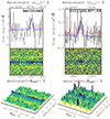 |
Fig. 5. Zoom-ins show two emission features detected in the VIS arm of the X-Shooter spectra. The left and right panels consist of the 1D continuum subtracted (upper), 2D (middle), and 3D (bottom) spectrograms of HeIIλ1640 with characteristic P-Cygni line profile and semi-forbidden non-resolved CIII]λλ1907,1909 line. The fitted Gaussian emission line is overplotted in blue. The 1D spectra in both panels is shown in black, error spectrum in red, and zero-level flux with the orange line. Sharp peaks notable in 1D around the CIII]λλ1907,1909 line belonging to the sky residuals are also visible in 2D and 3D spectrograms. The 1D and 2D spectrograms are displayed in rest and observed wavelength frame. |
3.2.2. X-Shooter NIR-arm
The NIR arm data were analyzed using a similar methodology as the VIS data described in the previous subsection. Upon our preliminary visual examination, the final stacked spectra observed from the NIR arm, covering the ∼2050 Å–4960 Å rest-frame range, show a very faint trace of continuum, visible down to ∼3500 Å. Faint [OII]λλ3727,3729 doublet with  and
and  flux was detected, confirming the systemic redshift of zspec = 3.999 ± 0.001 reported by Vanzella et al. (2018). We calculated the integrated flux from the lines by fitting the Gaussian line profile (using the same method described in Sect. 3.2.1), excluding the continuum-fitting procedure (as the continuum was extremely faint and negligibly contributing in this case). Furthermore, we binned the NIR data by a factor of 9, translating the spectrum from 0.5 Å/pix to 5.4 Å/pix resolution element to check for other fainter features, and show the resulting spectrum in Fig. 6. The [NeIII]λ3968 Å feature is clearly detected and partially blended with a skyline. To quantify the integrated flux of this line, we followed a methodology similar to that adopted for the [OII] doublet and other VIS lines. We first masked the skyline region (6 Å wide region) to prevent its interference with the Gaussian fitting process. Afterwards, we measured the integrated flux, as depicted in Fig. 7. The resulting flux is
 ![Mathematical equation: $ F_{\mathrm{[NeIII]}}=(1.56 \pm0.54)\times10^{-17}\,\rm erg/s/cm^2 $](/articles/aa/full_html/2025/06/aa51959-24/aa51959-24-eq9.gif) .
.
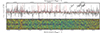 |
Fig. 6. Same as Fig. 4, but for the X-Shooter NIR-arm, showing the [OII]λλ3727,3729 doublet and [NeIII]λ3968 line. |
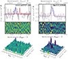 |
Fig. 7. Same as Fig. 5, but for the emission [OII]λλ3727,3729 doublet and [NeIII]λ3968 line detected in X-Shooter NIR spectrum. For the [OII]λλ3727,3729 doublet, the fitted Gaussian emission lines are overplotted in blue and red, respectively. The dashed red markers in [OII] 2D spectrogram point to the faint doublet at wavelengths [OII]λλ3727,3729. Spectrum in both panels are presented in black while error in red color and zero level flux with orange line. Note: the [NeIII]λ3968 line is partially blended with the skyline (gray shaded region of ∼6 Å width). The skyline is not taken into account when fitting a Gaussian curve and calculating the integrated line flux. The 1D and 2D spectrograms are displayed in the rest- and observed-frame wavelengths. |
4. Fraction of escaped LyC photons
We derived the relative escape fraction of Lyman continuum photons (fesc, rel) following Vanzella et al. (2012, 2018):
 (1)
(1)
where Lν(1500)/Lν(LyC) represents the intrinsic flux density ratio of non-ionizing UV radiation (in our case from λrest = 1400–1940 Å) and LyC photons, while Fν(1500)/Fν(LyC) refers to the observed flux density ratio. The  value takes into account the attenuation of LyC photons caused by the neutral hydrogen atoms along the line of sight.
From the HST F390W and F814W imaging the LyC flux blueward from 880 Å (the F390W band probes rest-frame range 700 − 880 Å, with a pivotal wavelength of 800 Å) and nonionizing flux at 1500 Å is measured  and Fν1500 = 7.6 ± 0.5 × 10⁻³⁰ erg/cm2/s/Hz, which correspond to flux density ratio of Fν(1500)/Fν(LyC) = 69 ± 19. On the other hand, the intrinsic luminosity ratio is sensitive to the choice of stellar population synthesis models and assumptions about key galaxy properties, including metallicity, age, star formation history, and initial mass function. This dependence can cause the Lν(1500)/Lν(LyC) ratio to vary significantly, from approximately 1.5–9, resulting in substantial uncertainty in the calculated escape fraction. Therefore, in order to put more stringent constraints on Lν(1500)/Lν(LyC), we can rely on the expression from Chisholm et al. (2019) that describes the relationship between stellar population age, metallicity, and the ratio between intrinsic ionizing and non-ionizing flux density:
 (2)
(2)
The presence of the NVλ1240 feature that shows a P-Cygni profile with clear absorption and emission (FORS spectra, Vanzella et al. 2018) is a strong indicator of young stellar populations (< 5 Myr) (Chisholm et al. 2019). The strength of the peak/through ratio can serve as an age indicator, where a higher ratio goes with younger ages. For Ion3, the estimated NVλ1240 peak/through ratio is ∼2.3, which corresponds to an age of ∼5 Myr, and with a given metallicity of 12 + log(O/H) = 8.02 ± 0.20 or ∼0.2 Z⊙, (see Sect. 5.4), we derived an intrinsic luminosity ratio of L(1500)/L(LyC) = 1.6 ± 0.9.
To fully sample the IGM transmission expected in F390W at z = 4.0, we simulated 10 000 mock sightlines using the prescription from Bassett et al. (2021). To summarize, the column density of HI in the IGM is modeled by randomly adding HI absorbers with column densities between 1012 and 1021 cm−2 to the mock sightlines using a column density distribution function given by Steidel et al. (2018). At wavelengths redder than 912 Å, these produce Voigt profiles, along with Doppler widths randomly sampled from Hui & Rutledge (1999). The first 32 Lyman series transitions are modeled. At bluer wavelengths, the absorption is proportional to NHIλ3 (e.g., Osterbrock 1974). In our simulations we did not include the CGM attenuation since the Ly-alpha multipeak line suggests a low-column-density of CGM (see Sect. 5.5). The resulting IGM transmission is shown as a function of wavelength in Fig. 8. We then integrated this through the F390W filter to model the probability distribution for the fraction of LyC photons from Ion3, which will pass through the IGM. This procedure is repeated for all 10 000 sightlines, with the resulting  distribution shown in Fig. 9.
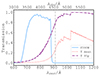 |
Fig. 8. Mean IGM transmission as a function of wavelength over 10 000 lines of sight is shown as a red dotted line. The purple dash dotted line is 95 percentile IGM transmission and the blue solid line represents the F390W filter curve. A vertical gray dashed line marks the beginning of LyC region at 912 Å. |
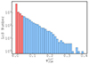 |
Fig. 9. Resulting distribution of IGM transmission for 10 000 sightlines. The blue part of the histogram marks the IGM transmission distribution of those sight lines, which (in combination with adopted intrinsic and observed flux ratio) result in fesc, rel = 0.06–1. The IGM transmissions shown in red result in fesc, rel > 1. |
To evaluate the relative escape fraction of ionizing photons, we adopted the previously estimated L(1500)/L(LyC) = 1.6 ± 0.9, Fν(1500)/Fν(LyC) = 69 ± 19 and the range of values for  shown as the blue part of histogram plot in Fig. 9. The values of
  , which produce fesc, rel > 1 (red histogram marked in Fig. 9) are not considered in the analysis. The corresponding distribution of fesc is shown in the histogram plot of Fig. 10 and spans the range fesc, rel = 0.06–1, depending on the
  . Finally it is worth noting that given the already large distribution of fesc values, we did not include LyC flux measurement uncertainty in the fesc, rel distribution in Fig. 10.
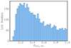 |
Fig. 10. Distribution of evaluated fesc, rel for Ion3 LyC leaker. The presented distribution only includes the |

5. Results and discussion
5.1. The electron density (ne) and ISM pressure (log(P/k))
To constrain the underlying physical conditions within the ISM (i.e., the electron density, electron temperature, pressure, metallicity, and ionization parameter), a variety of robust line diagnostics have been proposed. One of the most commonly used density diagnostics is the forbidden fine-structure [OII]λλ3727,3729 optical line doublet. The [OII] doublet is produced by collisional excitations and de-excitations; therefore, the [OII]λλ3727/3729 line ratio is sensitive to the electron density of the environments with T ∼ 1–2 × 10⁴ K, recognized as star-forming regions (Osterbrock & Ferland 2006). Furthermore, the [OII]λλ3727/3729 line ratio is a useful electron density diagnostic over the 40 − 10 000 cm−3 range, with errors up to 0.4 dex due to electron temperature dependency (for more details, we refer to Kewley et al. 2019).
We adopted the method of calculating ne described in Sanders et al. (2016), where the electron density is expressed as a function of the line ratio:
 (3)
(3)
where [OII]λλ3727/3729 line ratio is denoted as R and a = 0.3771, b = 2468, and c = 638.4 are the best fit coefficients. It is important to highlight that ne measurements are temperature-dependent, which can introduce errors of about ∼20% (Sanders et al. 2016). In our case, we adopted Te = 104 K (Osterbrock 1974). The uncertainty due to the relatively low signal to noise ratio of the [OII] components dominates the electron density measurement; therefore, any errors introduced by other effects are negligible. We found an electron density of ![Mathematical equation: $ n_{\mathrm{e}}^{[\rm OII]} = 2280\pm 1900 $](/articles/aa/full_html/2025/06/aa51959-24/aa51959-24-eq20.gif) cm−3, while using IRAFtemden task n
cm−3, while using IRAFtemden task n![Mathematical equation: $ _{\mathrm{e}}^{[\rm OII]} \sim 1340 $](/articles/aa/full_html/2025/06/aa51959-24/aa51959-24-eq21.gif) cm−3. The difference of ne as derived from Equation (3) and temden is expected, as shown in Fig. 1 of Sanders et al. (2016). Moreover, we derived a very similar electron density, namely,
cm−3. The difference of ne as derived from Equation (3) and temden is expected, as shown in Fig. 1 of Sanders et al. (2016). Moreover, we derived a very similar electron density, namely, ![Mathematical equation: $ n_{\mathrm{e}}^{[\rm OII]} = 2754 $](/articles/aa/full_html/2025/06/aa51959-24/aa51959-24-eq22.gif) cm−3, when using the theoretical relation between the [OII]λλ3729/3726 line ratio and electron density from Kewley et al. (2019), while the ISM pressure derived from the same theoretical relation results to be log(P/k) ∼7.89.
cm−3, when using the theoretical relation between the [OII]λλ3729/3726 line ratio and electron density from Kewley et al. (2019), while the ISM pressure derived from the same theoretical relation results to be log(P/k) ∼7.89.
Another density and pressure diagnostic we can use to probe the ISM physical conditions of Ion3 is the [CIII]λ1909/CIII]λ1906 line ratio (Kewley et al. 2019). This ratio is useful for diagnostics in environments characterized by high-pressure log(P/k) > 7.5 and high densities, in he range ne > 3 × 10³ − 5.5 × 105 cm−3. Therefore it is recognized as a more reliable tracer (in cases where more extreme conditions are present) than the [OII] diagnostic. The [CIII]λ1909 and CIII]λ1906 feature is clearly detected in the binned spectrum shown in Fig. 4. Figure 11, instead, shows the 2D non-binned zoomed spectrum of the same doublet. The two components CIII]λ1906 and [CIII]λ1909 are detected with S/Ns of 5.7 and 4.5, respectively, eventually providing a ratio [CIII]λ1909/CIII]λ1906 = 0.7 ± 0.3. Ratios lower than 1 suggest extreme ISM conditions, with  cm−3 and pressure of log(P/k) > 7.9.
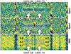 |
Fig. 11. Zoomed X-Shooter spectrum centerd on the CIII] doublet. Top: 2D spectrum at the original spectral resolution (R = 8900, 0.2 Å/pix) with the positions of the components indicated. Middle: Same spectrum as above with outlined the regions where the S/Ns were calculated in three spatial positions: below, above, and at the location of Ion3. The size of the boxes is 0.8″ × 250 km s−1. Bottom: 2D RMS spectrum is shown with reported the same boxes shown in the middle panel with listed the corresponding SN values. Detections emerge on top of Ion3 spatial position. |
It is worth noting that such extreme pressure values are typical of the most highly pressurized, turbulent medium in molecular clouds of local star-forming galaxies (Molina et al. 2020; Chevance et al. 2020) and high-redshift clumps in high-resolution simulations (Calura et al. 2022). In virialized systems such as star clusters, where equipartition between gravity and kinetic energy holds and where the gravitational pressure can be computed as Pgrav = G × Σ2, these P/k values correspond to gas surface density  /pc2. We also note that these values are by several orders of magnitude higher than the warm ISM in the Milky Way disk, characterized by typical thermal P/k
  cm−3. Overall results from [OII] and indications from [CIII]/CIII] line ratio diagnostics suggest that Ion3 has an extreme and dense ISM environment with high pressure. This suggests the formation and presence of very massive stars, a conclusion which is also supported by the large ionizing photon production efficiency, log(ξion/[Hz erg−1]) = 25.5, as measured in Vanzella et al. (2018) (see also, Schaerer et al. 2025). Deeper spectroscopic observations of CIII features are required to derive precise ratio among the components, however the current analysis suggest a ratio favoring a brighter blue component.
5.2. Unraveling the ISM ionization state of Ion3
The established empirical correlation between [NeIII]λ3870/[OII]λλ3727,29 and [OIII]λ5007/[OII]λλ3727,29 (O32) line ratios enables us to estimate the O32 index of Ion3, despite the lack of [OIII]λ5007 wavelength coverage in the data. The [NeIII]λ3968 emission line is detected in the X-Shooter spectrum, while the other component, [NeIII]λ3870, falls in a strong atmospheric absorption band1 and is absent in the spectrum. However, from the theoretical line ratio [NeIII]λ3870/[NeIII]λ3968 ∼ 2.4, we can estimate the flux of the [NeIII]λ3870, which results F![Mathematical equation: $ _{\mathrm{[NeIII]}}\sim 3.74 \times 10^{-17} \,\rm erg/s/cm^2 $](/articles/aa/full_html/2025/06/aa51959-24/aa51959-24-eq26.gif) , implying a significant large [NeIII]λ3870/[OII]λλ3727,29 ratio of 6.9 (Witstok et al. 2021). Adopting the empirical relationship (Equation (1), Witstok et al. 2021), the inferred line ratio would formally corresponds O32 > 100. Conservatively, we use the measured NeIII]λ3968 in place of [NeIII]λ3870, knowing that in this case the resulting O32 is a lower limit of > 50. Still, this value is significantly higher than the limiting ratio of O32 ≥ 5, characteristic of most other known LyC leakers at both low and high redshifts (Witstok et al. 2021). Furthermore, a high O32 line ratio is correlated with a high ionization parameter (log U), defined as the ratio of the number density of ionizing photons to the number density of particles. We derived log U using two methods, following the prescription from Díaz et al. (2000) and using the [NeIII]λ3870/[OII]λλ3727,29 ratio (Equation (3), Witstok et al. 2021). In both cases, the resulting ionization parameter was log U > −1.5, significantly higher than that of other known LyC leakers. Furthermore, comparing the log U of Ion3 with that of star-forming galaxies at high redshift, located in both lensed and non-lensed fields (Reddy et al. 2023a; Williams et al. 2023; Tang et al. 2023), the value we inferred is remarkably high – and comparable to the most extreme cases known in the local and high-z Universe (e.g., Jaskot et al. 2019; Topping et al. 2024). The ongoing intense starburst hosting young massive stars is consistent with extreme ISM conditions, whose estimated electron density is
, implying a significant large [NeIII]λ3870/[OII]λλ3727,29 ratio of 6.9 (Witstok et al. 2021). Adopting the empirical relationship (Equation (1), Witstok et al. 2021), the inferred line ratio would formally corresponds O32 > 100. Conservatively, we use the measured NeIII]λ3968 in place of [NeIII]λ3870, knowing that in this case the resulting O32 is a lower limit of > 50. Still, this value is significantly higher than the limiting ratio of O32 ≥ 5, characteristic of most other known LyC leakers at both low and high redshifts (Witstok et al. 2021). Furthermore, a high O32 line ratio is correlated with a high ionization parameter (log U), defined as the ratio of the number density of ionizing photons to the number density of particles. We derived log U using two methods, following the prescription from Díaz et al. (2000) and using the [NeIII]λ3870/[OII]λλ3727,29 ratio (Equation (3), Witstok et al. 2021). In both cases, the resulting ionization parameter was log U > −1.5, significantly higher than that of other known LyC leakers. Furthermore, comparing the log U of Ion3 with that of star-forming galaxies at high redshift, located in both lensed and non-lensed fields (Reddy et al. 2023a; Williams et al. 2023; Tang et al. 2023), the value we inferred is remarkably high – and comparable to the most extreme cases known in the local and high-z Universe (e.g., Jaskot et al. 2019; Topping et al. 2024). The ongoing intense starburst hosting young massive stars is consistent with extreme ISM conditions, whose estimated electron density is ![Mathematical equation: $ n_{\mathrm{e}}^{\mathrm{[OII]}} = 2280\pm1900 $](/articles/aa/full_html/2025/06/aa51959-24/aa51959-24-eq27.gif) cm−3 and
cm−3 and ![Mathematical equation: $ n_{\mathrm{e}}^{\mathrm{CIII]}} > 10^{4} $](/articles/aa/full_html/2025/06/aa51959-24/aa51959-24-eq28.gif) cm−3. However, in environments with a high electron density, the strength of low-ionization emission features can be suppressed due to increased collisional de-excitation, which can further affect the measured line ratios and inferred ionization parameter. Either way, both conditions require a hard ionization field generated from young massive stars, which is then responsible for the production of LyC radiation we have observed in the Hubble data.
cm−3. However, in environments with a high electron density, the strength of low-ionization emission features can be suppressed due to increased collisional de-excitation, which can further affect the measured line ratios and inferred ionization parameter. Either way, both conditions require a hard ionization field generated from young massive stars, which is then responsible for the production of LyC radiation we have observed in the Hubble data.
Finally, recent JWST observations of high redshift (z > 6) sources suggest that these extreme conditions may not be rare. For example, an extreme O32 = 184 has been reported at z > 6 by Topping et al. (2024). This source is recognized as a compact clump with the size of ∼20 pc having high SFR surface density, subsolar metallicity, and ISM under extreme ionization conditions with electron density and ionization parameters estimated to be ![Mathematical equation: $ n_{\mathrm{e}}^{\mathrm{CIII]}} = 1.1\times10{^5} $](/articles/aa/full_html/2025/06/aa51959-24/aa51959-24-eq29.gif) and log U ∼ −1, respectively. Similar conditions have been reported in another spectroscopically confirmed high-redshift galaxy, at z = 12.34 (GHZ2, Castellano et al. 2024; Calabrò et al. 2024). This galaxy is characterized by very high stellar and star-formation rate density, namely, 104 − 105M⊙ pc−2 and
and log U ∼ −1, respectively. Similar conditions have been reported in another spectroscopically confirmed high-redshift galaxy, at z = 12.34 (GHZ2, Castellano et al. 2024; Calabrò et al. 2024). This galaxy is characterized by very high stellar and star-formation rate density, namely, 104 − 105M⊙ pc−2 and  yr−1 kpc−2, respectively. Furthermore, the ISM of GHZ2 is characterized by low metallicity, < 0.1 Z⊙, a high ionizing parameter, log U > −2, and extreme ionizing conditions, with O32 ∼ 25. Ion3 shares similar physical properties of the ISM, observed during a young bursty event.
5.3. Star formation rate
Another key physical property that can be extracted from the forbidden [OII]λλ3727,3729 line (in this case, the dust-uncorrected line flux) is the star-formation rate (SFR), estimated as:
![Mathematical equation: $$ \begin{aligned} \mathrm {SFR}\,(\mathrm {M}_\odot \,yr^{-1}) = (1.4\pm 0.4)\times 10^{-41}\,L[OII]\,(erg\,s^{-1}), \end{aligned} $$](/articles/aa/full_html/2025/06/aa51959-24/aa51959-24-eq31.gif) (4)
(4)
where L[OII] is luminosity of the line. This prescription to derive the SFR from the [OII] forbidden line was adopted from Kennicutt (1998) and calibrated using the Hα line from two spectro-photometrical samples of galaxies (Gallagher et al. 1989; Kennicutt 1992). Gilbank et al. (2010) introduced an empirically-corrected SFR that takes into account metallicity and dust obscuration on [OII] as a function of galaxy mass:
![Mathematical equation: $$ \begin{aligned} \mathrm {SFR}([\mathrm {OII}])_{\mathrm {corr}} = \frac{\mathrm{SFR}_{[\mathrm {OII]}}}{\mathrm {a}\, \mathrm {tanh[(x-b)/c]+d}}, \end{aligned} $$](/articles/aa/full_html/2025/06/aa51959-24/aa51959-24-eq32.gif) (5)
(5)
where SFR[OII]= L([OII])/2.53 × 1040 ergs −1, x= log(M*/M⊙), a = −1.424, b = 9.827, c = 0.572, and d = 1.700. After adopting the above-mentioned empirical correction, we found SFR([OII])corr = 12 ± 5 M⊙ yr−1. Lastly, the SFR([OII]) value derived in this way was then additionally corrected by total magnification of 1.3, resulting in final SFR([OII]) M⊙ yr−1.
However, the [OII] SFR indicator is prone to substantial systematic uncertainties caused by different galaxy properties (ionization parameter, metallicity, extinction, etc., as given in Kennicutt 1998; Teplitz et al. 2003; Kewley et al. 2004; Moustakas et al. 2006), and differences in the SFR inferred from [OII] and Hα have been found to be as high as 0.5–1 dex (Kennicutt 1998; Kewley et al. 2004), namely, SFR([OII])corr can be subject to the large systematics.
On the other hand, the rest-frame UV nonionizing continuum is produced from stars with a broader mass range, extending down to a few M⊙. This implies that rest-frame UV flux traces SFR events over larger time periods of about 100 Myr. The inferred SFR(UV) from the F814W band probing the nonionizing ultraviolet luminosity is SFR(UV) = 10 ± 1 M⊙ yr−1 (Kennicutt & Evans 2012), where no dust attenuation is considered. To correct the SFR(UV) from dust extinction we applied the correction using A1600 – β relation: A1600 = 5.32−0.37+0.41 + 1.99 × β from Castellano et al. (2014), adopting β = −2.50 (Vanzella et al. 2018). The dust-corrected SFR is SFR(UV)corr∼ 14 M⊙ yr−1 and after applying magnification correction it decreases to ∼11 M⊙ yr−1.
A more reliable SFR tracer accessible for Ion3 is the Hα line. As discussed in Vanzella et al. (2018) Spitzer/IRAC photometry shows significant photometric excess in the 3.6 μm band, which includes the Hα line at its redshift. We derived the SFR(Hα) attributing this excess to Hα line. From the magnitude of the galaxy in the IRAC 3.6 μm band, mag = 23.20 ± 0.10 and subtracting the continuum (assumed from the nearest band, IRAC 4.5 μm, to be mag = 23.70 ± 0.10), we derived an Hα line flux  . The resulting SFR(Hα) is 100 ± 30 M⊙ yr−1 (Kennicutt & Evans 2012); after correcting for magnification, it is SFR(Hα)tot = 77 ± 23 M⊙ yr−1. The value presented here is slightly lower than that reported by Vanzella et al. (2018) (140 M⊙ yr−1), primarily because we have corrected for the continuum emission and assumed that the continuum level of 23.70 also applies to the IRAC 3.6 μm channel.
Hα is a nebular emission line produced by the recombination of gas ionized from short-living young and massive stars. Therefore, Hα is an excellent tracer of SFR events that span over short periods (< 10 Myr). The relatively high SFR(Hα) indicates Ion3 is undergoing an intense burst of star formation, in line with the detected LyC emission, steep ultraviolet slope, and signatures of massive stars in the ultraviolet spectrum (e.g., P-Cygni profile of NV). At the given stellar mass of ∼1.5 × 10⁹ M⊙, the SFR(Hα) places the LyC emitter Ion3 in the starburst phase, with a specific star formation rate of ≃70 Gyr−1, fully compatible with the strong Hα emitters observed during the epoch or reionization (e.g., Rinaldi et al. 2024). It worth reporting also the star formation rate surface density, ΣSFR, calculated as the ratio between the SFR(Hα) and the area outlined by the two-sigma contour defined in the F814W band (which probes the rest-frame non-ionizing ultraviolet radiation ∼1600 Å). Assuming the bulk of the SFR activity is confined within that area, corresponding to 5.5 kpc2 (see Fig. 3), ΣSFR is ≃20 M⊙ yr−1 kpc−2. This high value is consistent with the high electron density inferred above (Reddy et al. 2023a,b, see also Topping et al. 2025).
5.4. The CIII]λ λ1907,1909 metallicity
The CIII]λλ1907,1909 (CIII]λ1909) is a very useful spectral feature to identify very distant star-forming galaxies, for instance, at z > 6, especially in the pre-JWST era. (e.g., Shapley et al. 2003; Stark et al. 2014; Rigby et al. 2015; Ravindranath et al. 2020). Moreover, CIII]λ1909 proves to be a decent metallicity diagnostic for low-mass star-forming galaxies down to 12 + log(O/H) ∼7.5 (e.g., Rigby et al. 2015; Nakajima et al. 2018; Ravindranath et al. 2020; Mingozzi et al. 2022) and it is also considered as a potential tracer of LyC leaking galaxies, as shown for “Grean Pea” galaxies (Cardamone et al. 2009) with detected LyC emission (Schaerer et al. 2022; Izotov et al. 2023).
To evaluate the metallicity of Ion3, we are using the best fitting results of estimated gas-phase metallicities and measured (CIII]λ1909 from the sample of local high-z analogs. This is proven to be valid at 12 + log(O/H) > 7.5, with a scatter of 0.18 dex (Mingozzi et al. 2022):
![Mathematical equation: $$ \begin{aligned} 12+\mathrm {log(O/H)} = (-0.5\pm 0.13) \times \mathrm {log}(\mathrm {EW(CIII])})+(8.43\pm 0.11), \end{aligned} $$](/articles/aa/full_html/2025/06/aa51959-24/aa51959-24-eq35.gif) (6)
(6)
where EW(CIII]) is the rest-frame equivalent width of the doublet. The inferred EW(CIII]) = 6.5 Å reported in Sect. 3.2.1 implies a metallicity 12 + log(O/H) = 8.02 ± 0.20 or ∼0.2 Z⊙. This subsolar metallicity agrees with the measured values of other confirmed LyC leakers at high redshift, such as Ion2 (12 + log(O/H) = 8.07 ± 0.44, Vanzella et al. 2016; de Barros et al. 2016) and Sunburst (12 + log(O/H) ∼ 8.4, Rivera-Thorsen et al. 2017; Vanzella et al. 2020; Chisholm et al. 2019; Mainali et al. 2022; Meštrić et al. 2023).
5.5. Complexity of the Lyα line
Interpreting the properties of the Lyα line is challenging due to its resonant nature. The way how Lyα photons propagates through the ISM and CGM is affected by the intrinsic properties of the medium (e.g., geometry, ionization, and kinematics of the gas, dust attenuation, etc.) and leaves an imprint in the shape of the line. Therefore, Lyα is a carrier of valuable information about various intrinsic properties of the neutral hydrogen HI of the hosting galaxy. As a consequence of its nature, the Lyα profile is recognized as one of the most robust indirect tracers of escaping LyC photons (Verhamme et al. 2015), which was later proven on the basis of confirmed LyC emitters at various redshifts having complex Lyα profiles (Verhamme et al. 2017; Izotov et al. 2021b; Vanzella et al. 2020; Naidu et al. 2022); however, we also refer to the Ion1 LyC emitter at z = 3.8 without Lyα emission (Ji et al. 2020).
Figure 12 shows the complex Lyα multipeaked shape, in which a clear narrow emission close to the systemic redshift (red line) is evident (Lyα − systemic =dv ∼ −35 km s−1). In particular, including the uncertainty of the systemic redshift 3.999 ± 0.001, dv ranges from −60 to +10 km s−1, making the peak fully compatible with being at the systemic (dotted red lines in the same figure). The proximity of Lyα line location with its resonance frequency strongly indicates very low column density of neutral HI gas (e.g., Rivera-Thorsen et al. 2017; Behrens et al. 2014; Naidu et al. 2022), in line with the LyC detection reported in this work and suggesting the presence of ionized channels through which Lyα and LyC photons can escape into the IGM (Verhamme et al. 2017). It is worth noting that besides the presence of aligned ionized channels, there are ongoing radiative transfer effects that produce additional peaks observed far from the resonance frequency. This characteristic has also been observed in other confirmed leakers, such as the Sunburst arc at z = 2.37 (e.g., Vanzella et al. 2016) and among the local analogs, remarkably similar to the case of triple-peaked Lyα emitter J1243+4646 J1243+4646 (Izotov et al. 2018).
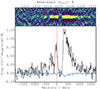 |
Fig. 12. 2D and the 1D spectra of the Lyα extracted from X-Shooter shown in the top and bottom panels. The blue line shows the spectrum of the sky, while the red vertical line (on the 1D spectrum) marks the systemic velocity of the source with the one sigma error (dotted vertical lines), located at +35 km s−1 form the central Lyα peak dubbed 0. The other Lyα peaks are marked as −2, −1 (blueward the systemic velocity), and 1 (redward from systemic velocity). |
6. Summary and conclusions
In this work, we present detailed HST multiband (F390W, F814W, and F140W) photometric and high-resolution VLT X-Shooter spectroscopic analysis of the most distant LyC leaker at zspec = 3.999, summarized in Table 1. The HST F390W band covers a clean non-contaminated portion of the LyC flux blueward ∼880 Å, while F814W covers the UV nonionizing part ∼1500 Å. Additional ancillary X-Shooter spectroscopy allowed us to investigate properties of spectroscopic features focusing on ∼CIVλ1550, HIIλ1640, CIII]λλ1907,1909, NeIII]λ3968, and [OII]λλ3726,3729. Our main results are summarized as follows:
-
We measured a non-contaminated LyC radiation using HST F390W band with S/N ∼ 3.5, which results in fesc, rel = 0.06–1, depending on the
 .
. -
Additional spectral features have been identified in the X-Shooter spectrum and confirmed the systemic redshift zspec = 3.999 ± 0.001, based on [OII]λλ3726,3729 and NeIII]λ3968 nebular features, revealing that within the uncertainties the Lyα central peak lies at the systemic velocity zsys. Furthermore, Ion3 shows signatures of an ongoing burst (P-Cygni profile of NV, rest-frame EW(Hα) ∼ 1000 Å and high [NeIII]λ3870/[OII]λλ3727,29 implying O32 > 50.
-
We find high electron density,
![Mathematical equation: $ n_{\mathrm{e}}^{\mathrm{[OII]}} = 2280\pm1900 $](/articles/aa/full_html/2025/06/aa51959-24/aa51959-24-eq37.gif) cm−3, indications for
cm−3, indications for ![Mathematical equation: $ n_{\mathrm{e}}^{\mathrm{CIII]}} > 10^{4} $](/articles/aa/full_html/2025/06/aa51959-24/aa51959-24-eq38.gif) cm−3 and subsolar metallicity 12 + log(O/H) = 8.02 ± 0.20, suggesting extreme ISM conditions connected with the high star-formation rate surface density.
cm−3 and subsolar metallicity 12 + log(O/H) = 8.02 ± 0.20, suggesting extreme ISM conditions connected with the high star-formation rate surface density. -
The star formation rate (SFR), has been evaluated, and corrected for magnification, using three different diagnostics ([OII], Hα, UV), yielded the following results: SFR([OII]) = 9 ± 4 M⊙ yr−1, SFR(Hα)
 , and SFR(UV)corr∼ 11 M⊙ yr−1. The star formation rate surface density of Ion3 is relatively high ΣSFR ≃ 20 M⊙ yr−1 kpc−2 and in line with the high electron density inferred in the steps described in Sect. 5.1.
 -
High-resolution HST imaging reveals the clumpy structure of Ion3. Using the F814W image, we measure the effective radius of Ion3A ∼ 180 pc, while an upper limit is derived for the second component, Ion3B < 100 pc, while the currently estimated area in the rest-frame 1600 Å is 5.5 kpc2.
This study presents a detailed analysis of Ion3, the most distant known LyC leaker, using deep HST imaging and X-Shooter spectroscopy to confirm LyC emission with a S/N of ∼3.5 and an estimated escape fraction ranging from 6% to 100%, depending on IGM attenuation. The galaxy exhibits a clumpy structure with high electron densities, subsolar metallicity, intense star formation, and evidence for high ionization conditions. These results indicate that Ion3 is being observed during a bursty star-forming episode when its ISM is optically thin to ionizing radiation. Further progress in investigating Ion3 will require spectroscopic observations of nebular lines with the JWST, which will help to confirm and strengthen the results presented in this work.
Acknowledgments
The authors thank the anonymous referee for helpful comments that improved the manuscript. We thank Rui Marques-Chaves on helpful discussion related to  . The analysis presented in this paper is based on observations with the NASA/ESA Hubble Space Telescope obtained at the Space Telescope Science Institute, which is operated by the Association of Universities for Research in Astronomy, Incorporated, under NASA contract NAS5-26555. Support for Program Number HST-GO-17133 was provided through a grant from the STScI under NASA contract NAS5-26555. UM, CG acknowledge financial support through grant PRIN-MUR 2020SKSTHZ M.M. acknowledges the financial support through grant PRIN-MIUR 2020SKSTHZ. MC acknowledges support from INAF Mini-grant “Reionization and Fundamental Cosmology with High-Redshift Galaxies”. AZ: The research activities described in this paper have been co-funded by the European Union – NextGenerationEU within PRIN 2022 project n.20229YBSAN – Globular clusters in cosmological simulations and in lensed fields: from their birth to the present epoch. AM acknowledges financial support through grant NextGenerationEU” RFF M4C2 1.1 PRIN 2022 project 2022ZSL4BL INSIGHT. KIC acknowledges funding from the Dutch Research Council (NWO) through the award of the Vici Grant VI.C.212.036. This research made use of Photutils, an Astropy package for detection and photometry of astronomical sources (Bradley et al. 2024). This work uses the following software packages: ASTROPY (Astropy Collaboration 2013; Price-Whelan et al. 2018), matplotlib (Hunter 2007), NUMPY (van der Walt et al. 2011); Harris et al. 2020), Python, (Van Rossum & Drake 2009), Scipy (Virtanen et al. 2020).
References
- Astropy Collaboration (Robitaille, T. P., et al.) 2013, A&A, 558, A33 [NASA ADS] [CrossRef] [EDP Sciences] [Google Scholar]
- Bassett, R., Ryan-Weber, E. V., Cooke, J., et al. 2021, MNRAS, 502, 108 [NASA ADS] [CrossRef] [Google Scholar]
- Behrens, C., Dijkstra, M., & Niemeyer, J. C. 2014, A&A, 563, A77 [NASA ADS] [CrossRef] [EDP Sciences] [Google Scholar]
- Bradley, L., Sipőcz, B., Robitaille, T., et al. 2024, https://doi.org/10.5281/zenodo.10967176 [Google Scholar]
- Calabrò, A., Castellano, M., Zavala, J. A., et al. 2024, ApJ, 975, 245 [CrossRef] [Google Scholar]
- Calura, F., Lupi, A., Rosdahl, J., et al. 2022, MNRAS, 516, 5914 [Google Scholar]
- Caminha, G. B., Grillo, C., Rosati, P., et al. 2016, A&A, 587, A80 [NASA ADS] [CrossRef] [EDP Sciences] [Google Scholar]
- Cardamone, C., Schawinski, K., Sarzi, M., et al. 2009, MNRAS, 399, 1191 [NASA ADS] [CrossRef] [Google Scholar]
- Castellano, M., Sommariva, V., Fontana, A., et al. 2014, A&A, 566, A19 [NASA ADS] [CrossRef] [EDP Sciences] [Google Scholar]
- Castellano, M., Napolitano, L., Fontana, A., et al. 2024, ApJ, 972, 143 [Google Scholar]
- Chevance, M., Kruijssen, J. M. D., Vazquez-Semadeni, E., et al. 2020, Space Sci. Rev., 216, 50 [NASA ADS] [CrossRef] [Google Scholar]
- Chisholm, J., Rigby, J. R., Bayliss, M., et al. 2019, ApJ, 882, 182 [Google Scholar]
- de Barros, S., Vanzella, E., Amorín, R., et al. 2016, A&A, 585, A51 [NASA ADS] [CrossRef] [EDP Sciences] [Google Scholar]
- Díaz, A. I., Castellanos, M., Terlevich, E., & Luisa García-Vargas, M. 2000, MNRAS, 318, 462 [CrossRef] [Google Scholar]
- Finkelstein, S. L., D’Aloisio, A., Paardekooper, J.-P., et al. 2019, ApJ, 879, 36 [Google Scholar]
- Fletcher, T. J., Tang, M., Robertson, B. E., et al. 2019, ApJ, 878, 87 [Google Scholar]
- Flury, S. R., Jaskot, A. E., Ferguson, H. C., et al. 2022, ApJS, 260, 1 [NASA ADS] [CrossRef] [Google Scholar]
- Gaia Collaboration (Vallenari, A., et al.) 2023, A&A, 674, A1 [NASA ADS] [CrossRef] [EDP Sciences] [Google Scholar]
- Gallagher, J. S., Bushouse, H., & Hunter, D. A. 1989, AJ, 97, 700 [Google Scholar]
- Gilbank, D. G., Baldry, I. K., Balogh, M. L., Glazebrook, K., & Bower, R. G. 2010, MNRAS, 405, 2594 [NASA ADS] [Google Scholar]
- Gonzaga, S., Hack, W., Fruchter, A., & Mack, J. 2012, The DrizzlePac Handbook [Google Scholar]
- Harris, C. R., Millman, K. J., van der Walt, S. J., et al. 2020, Nature, 585, 357 [NASA ADS] [CrossRef] [Google Scholar]
- Hoffmann, S. L., Mack, J., Avila, R., et al. 2021, Am. Astron. Soc. Meet. Abstr., 53, 216.02 [Google Scholar]
- Hui, L., & Rutledge, R. E. 1999, ApJ, 517, 541 [Google Scholar]
- Hunter, J. D. 2007, Comput. Sci. Eng., 9, 90 [NASA ADS] [CrossRef] [Google Scholar]
- Inoue, A. K., & Iwata, I. 2008, MNRAS, 387, 1681 [Google Scholar]
- Inoue, A. K., Shimizu, I., Iwata, I., & Tanaka, M. 2014, MNRAS, 442, 1805 [NASA ADS] [CrossRef] [Google Scholar]
- Izotov, Y. I., Schaerer, D., Worseck, G., et al. 2018, MNRAS, 474, 4514 [Google Scholar]
- Izotov, Y. I., Worseck, G., Schaerer, D., et al. 2021a, MNRAS, 503, 1734 [NASA ADS] [CrossRef] [Google Scholar]
- Izotov, Y. I., Guseva, N. G., Fricke, K. J., et al. 2021b, A&A, 646, A138 [NASA ADS] [CrossRef] [EDP Sciences] [Google Scholar]
- Izotov, Y. I., Schaerer, D., Worseck, G., et al. 2023, MNRAS, 522, 1228 [NASA ADS] [CrossRef] [Google Scholar]
- Jaskot, A. E., Dowd, T., Oey, M. S., Scarlata, C., & McKinney, J. 2019, ApJ, 885, 96 [Google Scholar]
- Jaskot, A. E., Silveyra, A. C., Plantinga, A., et al. 2024a, ApJ, 972, 92 [NASA ADS] [CrossRef] [Google Scholar]
- Jaskot, A. E., Silveyra, A. C., Plantinga, A., et al. 2024b, ApJ, 973, 111 [NASA ADS] [CrossRef] [Google Scholar]
- Ji, Z., Giavalisco, M., Vanzella, E., et al. 2020, ApJ, 888, 109 [Google Scholar]
- Kennicutt, R. C. Jr. 1992, ApJ, 388, 310 [CrossRef] [Google Scholar]
- Kennicutt, R. C. Jr. 1998, ARA&A, 36, 189 [NASA ADS] [CrossRef] [Google Scholar]
- Kennicutt, R. C., & Evans, N. J. 2012, ARA&A, 50, 531 [NASA ADS] [CrossRef] [Google Scholar]
- Kewley, L. J., Geller, M. J., & Jansen, R. A. 2004, AJ, 127, 2002 [Google Scholar]
- Kewley, L. J., Nicholls, D. C., Sutherland, R., et al. 2019, ApJ, 880, 16 [Google Scholar]
- Lotz, J. M., Koekemoer, A., Coe, D., et al. 2017, ApJ, 837, 97 [Google Scholar]
- Mainali, R., Rigby, J. R., Chisholm, J., et al. 2022, ApJ, 940, 160 [NASA ADS] [CrossRef] [Google Scholar]
- Marinelli, M., & Dressel, L. 2024, WFC3 Instrument Handbook for Cycle 32 v. 16 (Baltimore, MD: Space Telescope Science Institute), 16, 16 [Google Scholar]
- Marques-Chaves, R., Schaerer, D., Álvarez-Márquez, J., et al. 2021, MNRAS, 507, 524 [NASA ADS] [CrossRef] [Google Scholar]
- Marques-Chaves, R., Schaerer, D., Álvarez-Márquez, J., et al. 2022, MNRAS, 517, 2972 [CrossRef] [Google Scholar]
- Meštrić, U., Vanzella, E., Zanella, A., et al. 2022, MNRAS, 516, 3532 [CrossRef] [Google Scholar]
- Meštrić, U., Vanzella, E., Upadhyaya, A., et al. 2023, A&A, 673, A50 [NASA ADS] [CrossRef] [EDP Sciences] [Google Scholar]
- Mingozzi, M., James, B. L., Arellano-Córdova, K. Z., et al. 2022, ApJ, 939, 110 [NASA ADS] [CrossRef] [Google Scholar]
- Molina, J., Ibar, E., Godoy, N., et al. 2020, A&A, 643, A78 [NASA ADS] [CrossRef] [EDP Sciences] [Google Scholar]
- Moustakas, J., Kennicutt, R. C. Jr., & Tremonti, C. A. 2006, ApJ, 642, 775 [NASA ADS] [CrossRef] [Google Scholar]
- Naidu, R. P., Tacchella, S., Mason, C. A., et al. 2020, ApJ, 892, 109 [NASA ADS] [CrossRef] [Google Scholar]
- Naidu, R. P., Matthee, J., Oesch, P. A., et al. 2022, MNRAS, 510, 4582 [CrossRef] [Google Scholar]
- Nakajima, K., Schaerer, D., Le Fèvre, O., et al. 2018, A&A, 612, A94 [NASA ADS] [CrossRef] [EDP Sciences] [Google Scholar]
- Nestor, D. B., Shapley, A. E., Steidel, C. C., & Siana, B. 2011, ApJ, 736, 18 [NASA ADS] [CrossRef] [Google Scholar]
- Osterbrock, D. E. 1974, Astrophysics of Gaseous Nebulae (San Franciso: Freeman) [Google Scholar]
- Osterbrock, D. E., & Ferland, G. J. 2006, Astrophysics of Gaseous Nebulae and Active Galactic Nuclei (Sausalito, CA: University Science Books) [Google Scholar]
- Peng, C. Y., Ho, L. C., Impey, C. D., & Rix, H.-W. 2002, AJ, 124, 266 [Google Scholar]
- Peng, C. Y., Ho, L. C., Impey, C. D., & Rix, H.-W. 2010, AJ, 139, 2097 [Google Scholar]
- Price-Whelan, A. M., Sipőcz, B. M., Günther, H. M., et al. 2018, AJ, 156, 123 [NASA ADS] [CrossRef] [Google Scholar]
- Prichard, L. J., Rafelski, M., Cooke, J., et al. 2022, ApJ, 924, 14 [Google Scholar]
- Ravindranath, S., Monroe, T., Jaskot, A., Ferguson, H. C., & Tumlinson, J. 2020, ApJ, 896, 170 [NASA ADS] [CrossRef] [Google Scholar]
- Reddy, N. A., Topping, M. W., Sanders, R. L., Shapley, A. E., & Brammer, G. 2023a, ApJ, 952, 167 [CrossRef] [Google Scholar]
- Reddy, N. A., Sanders, R. L., Shapley, A. E., et al. 2023b, ApJ, 951, 56 [NASA ADS] [CrossRef] [Google Scholar]
- Revalski, M., Rafelski, M., Fumagalli, M., et al. 2023, ApJS, 265, 40 [NASA ADS] [CrossRef] [Google Scholar]
- Rigby, J. R., Bayliss, M. B., Gladders, M. D., et al. 2015, ApJ, 814, L6 [NASA ADS] [CrossRef] [Google Scholar]
- Rinaldi, P., Caputi, K. I., Iani, E., et al. 2024, ApJ, 969, 12 [NASA ADS] [CrossRef] [Google Scholar]
- Rivera-Thorsen, T. E., Dahle, H., Gronke, M., et al. 2017, A&A, 608, L4 [NASA ADS] [CrossRef] [EDP Sciences] [Google Scholar]
- Rivera-Thorsen, T. E., Dahle, H., Chisholm, J., et al. 2019, Science, 366, 738 [Google Scholar]
- Sanders, R. L., Shapley, A. E., Kriek, M., et al. 2016, ApJ, 816, 23 [Google Scholar]
- Schaerer, D., Izotov, Y. I., Worseck, G., et al. 2022, A&A, 658, L11 [NASA ADS] [CrossRef] [EDP Sciences] [Google Scholar]
- Schaerer, D., Guibert, J., Marques-Chaves, R., & Martins, F. 2025, A&A, 693, A271 [NASA ADS] [CrossRef] [EDP Sciences] [Google Scholar]
- Shapley, A. E., Steidel, C. C., Pettini, M., & Adelberger, K. L. 2003, ApJ, 588, 65 [Google Scholar]
- Shapley, A. E., Steidel, C. C., Strom, A. L., et al. 2016, ApJ, 826, L24 [Google Scholar]
- Simmonds, C., Tacchella, S., Hainline, K., et al. 2024, MNRAS, 527, 6139 [Google Scholar]
- Stark, D. P., Richard, J., Siana, B., et al. 2014, MNRAS, 445, 3200 [NASA ADS] [CrossRef] [Google Scholar]
- Steidel, C. C., Bogosavljević, M., Shapley, A. E., et al. 2018, ApJ, 869, 123 [Google Scholar]
- Tang, M., Stark, D. P., Chen, Z., et al. 2023, MNRAS, 526, 1657 [NASA ADS] [CrossRef] [Google Scholar]
- Teplitz, H. I., Collins, N. R., Gardner, J. P., Hill, R. S., & Rhodes, J. 2003, ApJ, 589, 704 [Google Scholar]
- Topping, M. W., Stark, D. P., Senchyna, P., et al. 2024, MNRAS, 529, 3301 [NASA ADS] [CrossRef] [Google Scholar]
- Topping, M. W., Sanders, R. L., Shapley, A. E., et al. 2025, ArXiv e-prints [arXiv:2502.08712] [Google Scholar]
- van der Walt, S., Colbert, S. C., & Varoquaux, G. 2011, Comput. Sci. Eng., 13, 22 [Google Scholar]
- van Dokkum, P. G. 2001, PASP, 113, 1420 [Google Scholar]
- Van Rossum, G., & Drake, F. L. 2009, Python 3 Reference Manual (Scotts Valley, CA: CreateSpace) [Google Scholar]
- Vanzella, E., Siana, B., Cristiani, S., & Nonino, M. 2010, MNRAS, 404, 1672 [NASA ADS] [Google Scholar]
- Vanzella, E., Guo, Y., Giavalisco, M., et al. 2012, ApJ, 751, 70 [NASA ADS] [CrossRef] [Google Scholar]
- Vanzella, E., de Barros, S., Vasei, K., et al. 2016, ApJ, 825, 41 [NASA ADS] [CrossRef] [Google Scholar]
- Vanzella, E., Nonino, M., Cupani, G., et al. 2018, MNRAS, 476, L15 [Google Scholar]
- Vanzella, E., Caminha, G. B., Calura, F., et al. 2020, MNRAS, 491, 1093 [Google Scholar]
- Verhamme, A., Orlitová, I., Schaerer, D., & Hayes, M. 2015, A&A, 578, A7 [NASA ADS] [CrossRef] [EDP Sciences] [Google Scholar]
- Verhamme, A., Orlitová, I., Schaerer, D., et al. 2017, A&A, 597, A13 [NASA ADS] [CrossRef] [EDP Sciences] [Google Scholar]
- Virtanen, P., Gommers, R., Oliphant, T. E., et al. 2020, Nat. Methods, 17, 261 [Google Scholar]
- Wang, X., Teplitz, H. I., Sun, L., et al. 2024, Res. Notes Am. Astron. Soc., 8, 26 [Google Scholar]
- Williams, H., Kelly, P. L., Chen, W., et al. 2023, Science, 380, 416 [NASA ADS] [CrossRef] [Google Scholar]
- Witstok, J., Smit, R., Maiolino, R., et al. 2021, MNRAS, 508, 1686 [NASA ADS] [CrossRef] [Google Scholar]
- Worseck, G., Prochaska, J. X., O’Meara, J. M., et al. 2014, MNRAS, 445, 1745 [NASA ADS] [CrossRef] [Google Scholar]
All Tables
All Figures
|
Fig. 1. Left: HST F390W band thumbnail image of Ion3, size 5″ × 5″. Three zoom-in cut outs of sizes 1.5″ × 1.5″ are shown on the right side and F390W, F814W, and F140W bands with their expected PSFs in the upper left corner, blue circle. The HST F390W band probes LyC flux from 890 Å and blueward (note: the F390W band misses the first ∼20 Å of LyC flux). Green arrows point toward two clumpy structures (A and B) at z = 3.999 where LyC flux is detected. The third clumpy structure, pointed to with a purple arrow (C), very close to the LyC leaking sources, is most likely a low-z interloper, which is masked before the LyC flux is measured. Finally, the blue circle is adopted as the aperture to measure LyC flux, with a diameter of 0.36″, while the cyan rectangle (D) encloses the source that probably contaminates the LyC flux detected from the FORS spectroscopy. The blue lines indicate the VLT FORS slit position, showing that source D enters the slit and likely contaminates the LyC flux detected in FORS spectroscopy. The grey lines show the VLT X-Shooter slit position. The second observed band is F814W and covers non-ionizing UV flux, where both LyC leaking clumps are detected. The third panel is the F140W band, where Ion3 is detected as a single bright blob, which is not resolved due to the lower spatial resolution of WFC3/IR. The three small green diamonds are centered on the clumpy sources A, B, and C in the F390W image, with their corresponding positions also shown in the F814W and F140W images. It is noticeable that clump A detected in F390W is slightly offset from clump A observed in F814W. |
| In the text | |
|
Fig. 2. Histogram density plot of randomly placed 10 000 apertures over a 5″ × 5″ F390W image centered on Ion3. The black line is the Gaussian fit to the measured fluxes (in ADU) from 10 k apertures, with a resulting mean value of 0.001 and a 1σ of 0.0119, marked with a red dashed line (2σ and 3σ are marked with yellow and green dashed lines, respectively). The thick blue dashed line represents the background-subtracted, clean, non-contaminated LyC signal of Ion3, while thin gray dashed line is measured non-contaminated LyC signal before the background subtraction. |
| In the text | |
|
Fig. 3. Results from Galfit modeling. The first panel shows the original F814W image of Ion3 covering the non-ionizing UV flux with 2σ contour in red, also overlaid in other two panels. The second panel is the resulting model from Galfit and the third panel is a residual map. |
| In the text | |
|
Fig. 4. X-Shooter VIS-arm 1D spectra (upper panel) and 2D spectra (bottom panel) covering the rest-UV wavelengths from ∼1180 Å–1940 Å. The spectrum (black) is binned by a factor of 9 to increase the S/N of the continuum and other spectroscopic features, while 1σ uncertainty is presented in red color and orange line shows 0 flux level. The displayed 1D spectrum is continuum subtracted. The location of the reported and analyzed emission features (HeIIλ1640 and CIII]λλ1907,1909) are marked with thick black markers, while the positions of the other lines reported in Vanzella et al. (2018) from FORS spectroscopy (Lyα, NVλ1240, [CII]λ1335.71, [SIV]λλ1393,1402, CIVλλ1548,1550) are marked with thin blue markers. |
| In the text | |
|
Fig. 5. Zoom-ins show two emission features detected in the VIS arm of the X-Shooter spectra. The left and right panels consist of the 1D continuum subtracted (upper), 2D (middle), and 3D (bottom) spectrograms of HeIIλ1640 with characteristic P-Cygni line profile and semi-forbidden non-resolved CIII]λλ1907,1909 line. The fitted Gaussian emission line is overplotted in blue. The 1D spectra in both panels is shown in black, error spectrum in red, and zero-level flux with the orange line. Sharp peaks notable in 1D around the CIII]λλ1907,1909 line belonging to the sky residuals are also visible in 2D and 3D spectrograms. The 1D and 2D spectrograms are displayed in rest and observed wavelength frame. |
| In the text | |
|
Fig. 6. Same as Fig. 4, but for the X-Shooter NIR-arm, showing the [OII]λλ3727,3729 doublet and [NeIII]λ3968 line. |
| In the text | |
|
Fig. 7. Same as Fig. 5, but for the emission [OII]λλ3727,3729 doublet and [NeIII]λ3968 line detected in X-Shooter NIR spectrum. For the [OII]λλ3727,3729 doublet, the fitted Gaussian emission lines are overplotted in blue and red, respectively. The dashed red markers in [OII] 2D spectrogram point to the faint doublet at wavelengths [OII]λλ3727,3729. Spectrum in both panels are presented in black while error in red color and zero level flux with orange line. Note: the [NeIII]λ3968 line is partially blended with the skyline (gray shaded region of ∼6 Å width). The skyline is not taken into account when fitting a Gaussian curve and calculating the integrated line flux. The 1D and 2D spectrograms are displayed in the rest- and observed-frame wavelengths. |
| In the text | |
|
Fig. 8. Mean IGM transmission as a function of wavelength over 10 000 lines of sight is shown as a red dotted line. The purple dash dotted line is 95 percentile IGM transmission and the blue solid line represents the F390W filter curve. A vertical gray dashed line marks the beginning of LyC region at 912 Å. |
| In the text | |
|
Fig. 9. Resulting distribution of IGM transmission for 10 000 sightlines. The blue part of the histogram marks the IGM transmission distribution of those sight lines, which (in combination with adopted intrinsic and observed flux ratio) result in fesc, rel = 0.06–1. The IGM transmissions shown in red result in fesc, rel > 1. |
| In the text | |
|
Fig. 10. Distribution of evaluated fesc, rel for Ion3 LyC leaker. The presented distribution only includes the |
| In the text | |
|
Fig. 11. Zoomed X-Shooter spectrum centerd on the CIII] doublet. Top: 2D spectrum at the original spectral resolution (R = 8900, 0.2 Å/pix) with the positions of the components indicated. Middle: Same spectrum as above with outlined the regions where the S/Ns were calculated in three spatial positions: below, above, and at the location of Ion3. The size of the boxes is 0.8″ × 250 km s−1. Bottom: 2D RMS spectrum is shown with reported the same boxes shown in the middle panel with listed the corresponding SN values. Detections emerge on top of Ion3 spatial position. |
| In the text | |
|
Fig. 12. 2D and the 1D spectra of the Lyα extracted from X-Shooter shown in the top and bottom panels. The blue line shows the spectrum of the sky, while the red vertical line (on the 1D spectrum) marks the systemic velocity of the source with the one sigma error (dotted vertical lines), located at +35 km s−1 form the central Lyα peak dubbed 0. The other Lyα peaks are marked as −2, −1 (blueward the systemic velocity), and 1 (redward from systemic velocity). |
| In the text | |
Current usage metrics show cumulative count of Article Views (full-text article views including HTML views, PDF and ePub downloads, according to the available data) and Abstracts Views on Vision4Press platform.
Data correspond to usage on the plateform after 2015. The current usage metrics is available 48-96 hours after online publication and is updated daily on week days.
Initial download of the metrics may take a while.