| Issue |
A&A
Volume 698, June 2025
|
|
|---|---|---|
| Article Number | A295 | |
| Number of page(s) | 11 | |
| Section | Catalogs and data | |
| DOI | https://doi.org/10.1051/0004-6361/202451807 | |
| Published online | 27 June 2025 | |
Selected open cluster sample for validating atmospheric parameters: Application to Gaia and other surveys
1
Astrophysics Division, Shanghai Astronomical Observatory, Chinese Academy of Sciences,
80 Nandan Road,
Shanghai
200030,
PR China
2
School of Astronomy and Space Science, University of Chinese Academy of Sciences,
No. 19A, Yuquan Road,
Beijing
100049,
PR China
3
Institut de Ciències del Cosmos, Universitat de Barcelona (ICCUB),
Martí i Franquès 1,
08028
Barcelona,
Spain
★ Corresponding author: This email address is being protected from spambots. You need JavaScript enabled to view it.
Received:
6
August
2024
Accepted:
6
May
2025
Abstract
Context. Reliable stellar atmospheric parameters are essential for probing stellar structure and evolution, and for stellar population studies. However, various deviations appear in comparisons with different ground-based spectroscopic surveys.
Aims. We aim to select high-quality open cluster members and employ the atmospheric parameters provided by the theoretical isochrones of open clusters as a benchmark to assess the quality of stellar atmospheric parameters from Gaia DR3 and other ground-based spectroscopic surveys, such as LAMOST DR11, APOGEE DR17, and GALAH DR4.
Methods. We selected 130 open clusters with well-defined main sequences within 500 pc of the solar neighborhood as a benchmark sample to estimate the reference atmospheric parameters of the members from the best-fit isochrones of those clusters.
Results. By comparing the atmospheric parameters provided by different spectroscopic surveys to the theoretical parameters, we found that the atmospheric parameter deviation and the corresponding dispersions exhibit different variations. The atmospheric parameter deviations of F, G, and K-type stars are smaller than those of B, A, and M-type stars for most surveys. For most samples, the dispersion of Teff decreases as temperature decreases, whereas the dispersion of g shows the opposite trend.
Key words: surveys / stars: fundamental parameters / Hertzsprung-Russell and C-M diagrams / open clusters and associations: general
© The Authors 2025
 Open Access article, published by EDP Sciences, under the terms of the Creative Commons Attribution License (https://creativecommons.org/licenses/by/4.0), which permits unrestricted use, distribution, and reproduction in any medium, provided the original work is properly cited.
This article is published in open access under the Subscribe to Open model. This email address is being protected from spambots. You need JavaScript enabled to view it. to support open access publication.
1 Introduction
Stellar spectra allow us to obtain basic stellar atmospheric parameters, such as the effective temperature (Teff), the surface gravity (log g), and the metallicity ([M/H]) (Wu et al. 2011; Blanco-Cuaresma et al. 2014). This information is essential not only for exploring stellar formation and evolution but also for understanding the structure and formation history of the Milky Way (Fu et al. 2022; Netopil et al. 2022).
The ambitious European Space Agency (ESA)mission Gaia (Gaia Collaboration 2016) has provided insights into the physical properties of Milky Way stars. Gaia Data Release 3 (DR3, Gaia Collaboration 2023) published high-precision astrometric, photometric, and atmospheric parameters for a vast number of stars, which revolutionized the study of stars and the Milky Way. The General Stellar Parameterizer from Photometry (GSP-Phot) is an important module that aims to estimate atmospheric param- eters from low-resolution blue photometer (BP) and red photometer (RP) spectra. It provided the atmospheric parameters, including Teff, log g, and [M/H], for about 470 million sources (Creevey et al. 2023; Andrae et al. 2023). Meanwhile, Gaia DR3 has released low-resolution BP/RP spectra (λ/Δλ = 20−60) covering wavelength ranges of 330−680 nm and 640−1050 nm for approximately 220 million stars with sufficient observation times and high signal-to-noise ratios (De Angeli et al. 2023). The General Stellar Parameterizer from Spectroscopy (GSP-Spec) is another crucial module of the Gaia mission, estimating the chemophysical parameters for about 5.6 million stars using the pure spectroscopic processing of the Radial Velocity Spectrometer (RVS) (λ/Δλ ∼ 11 500), which covers the wavelength range of 846−870 nm (Recio-Blanco et al. 2023). Moreover, the Extended Stellar Parameterizer for Hot Stars (ESP-HS), a module dedicated to analyzing high-temperature stars (O, B, and A-type stars), provided atmospheric parameters for about 2.4 million stars (Fouesneau et al. 2023, hereafter (F23)). It is noted that the Gaia methods do not incorporate prior information like binary stars, member stars, or known distances when estimating these atmospheric parameters on a star-by-star basis from the observational data. Also, in dense regions there could be issues in the BP, RP, and RVS astrometric data because of the limits in the angular resolution.
Other spectroscopic surveys also provide a large sample of atmospheric parameters, such as the Large Sky Area Multi-Object Fiber Spectroscopic Telescope survey (LAMOST, Cui et al. 2012; Zhao et al. 2012), the Apache Point Observatory Galactic Evolution Experiment survey (APOGEE, Majewski et al. 2017), and the GALactic Archaeology with HERMES survey (GALAH, Buder et al. 2021). The LAMOST Low-Resolution Spectroscopic Survey provided a stellar parameter catalog for about 7.7 million A, F, G, and K-type stars (LAMOST-LRS DR11 v1.01) from the LAMOST Stellar Parameter Pipeline (LASP, Wu et al. 2011). The published low-resolution spectra (λ/Δλ ∼ 1800) cover the wavelength range of 370–900 nm. The most current APOGEE data release 17 (DR17, Abdurro’uf et al. 2022) includes spectroscopic parameters determined by the APOGEE Stellar Parameters and Chemical Abundances Pipeline (ASPCAP, García Pérez et al. 2016) for more than 730 000 stars with high-resolution spectra (λ/Δλ ∼ 22 500, 1510–1700 nm). The fourth data release (DR4, Buder et al. 2024) of the GALAH survey contains stellar parameters provided by Spectroscopy Made Easy (SME, Valenti & Piskunov 2012) for 917 588 stars from high-resolution spectra with four noncontiguous wavelength bands in the range of 471−490, 565−587, 648−674, and 759−789 nm.
Several recent studies have compared the Gaia atmospheric data with other survey data. Andrae et al. (2023) compared GSP-Phot parameters to those from APOGEE DR16, GALAH DR3, LAMOST DR4, and RAVE DR6, obtaining median absolute differences of 169 K, 110 K, 110 K, and 160 K for Teff and 0.22 dex, 0.06 dex, 0.1 dex, and 0.25 dex for log g, respectively. They suggested that GSP-Phot tends to overestimate Teff in the Galactic plane (see their Fig. 8) and systematically overestimates log g (see their Fig. 9). Recio-Blanco et al. (2023) compared GSP-Spec parameters with APOGEE DR17, GALAH DR3, and RAVE DR6 with a selected best-quality sample. They determined a median offset for Teff and log g of −17 K and −0.3 dex, respectively. F23 compared the ESP-HS parameters for hot stars with some literature catalogs. They found that the dispersions in Teff and log g deviation values between the ESP-HS and other catalogs increased with temperature. These parameters obtained from different spectroscopic surveys vary in the observed band, spectral resolution, and data processing method, which may lead to some systematic differences. For example, the deviation and dispersion of Teff between GSP-Phot and APOGEE DR16 are 2–3 times greater than those between GSP-Phot and LAMOST DR4, GALAH DR3, and RAVE DR6. Therefore, it is a challenge to accurately assess the quality of the atmospheric parameters of the different surveys.
To test the diverse systematic deviations among different spectroscopic surveys, we employed the atmospheric parameters from PARSEC isochrones (Marigo et al. 2017) as a benchmark to assess the observational atmospheric parameters of Gaia DR3, LAMOST-LRS DR11, APOGEE DR17, and GALAH DR4. Compared with field stars, it is noted that open clusters can be used as a bridge between observation and theoretical parameters, which are highly efficient for evaluating the quality of stellar parameters (Zhong et al. 2020; Fu et al. 2022; Fouesneau et al. 2023). This is because the member stars in an open cluster are formed in the same molecular cloud, sharing a similar age, metallicity, distance, and extinction (Lada & Lada 2003; Portegies Zwart et al. 2010), and so can be obtained with a more accurate age through isochrone fitting (Monteiro et al. 2010; Bossini et al. 2019). After determining the stellar age, their parameter values, such as the Teff and log g of cluster members, can be estimated by comparing the PARSEC isochrones and their locus on the color-magnitude diagrams (CMDs).
The unprecedented precise astrometric and photometric from Gaia data (Gaia Collaboration 2023), together with the popularity of machine learning approaches (Krone-Martins & Moitinho 2014; Pera et al. 2021; McInnes et al. 2017; Hunt & Reffert 2021) in finding the open cluster, has effectively boosted the cluster census and the reliability of membership determination. More than 4000 open clusters have been detected in the Milky Way (Cantat-Gaudin et al. 2018, 2020; Liu & Pang 2019; Sim et al. 2019; Castro-Ginard et al. 2020, 2022; Qin et al. 2021, 2023; He et al. 2022a, b; Hunt & Reffert 2023), which offers us an opportunity to evaluate the atmospheric parameters from Gaia DR3 with a large and reliable sample of member stars.
F23 estimated reference values of atmospheric parameters from isochrone fitting for 230 000 cluster members and compared the atmospheric parameters provided by Gaia DR3. They obtained a median of residuals to the isochrones for Teff, log g from GSP-Phot of 34 K, 0.01 dex, respectively, and a mean absolute deviation (MAD) of 400 K, 0.22 dex. They also pointed out the overestimation of Teff for giants and log g for the main sequence stars and the underestimation of Teff for supergiants and log g for hot stars and giants. When comparing the atmospheric parameters of GSP-Spec with the reference values, they found a median and a MAD of Teff, log g residuals to the isochrones of 6 K and 160 K, 0.3 dex and 0.44 dex, respectively. They also noted a systematic underestimation of both Teff and log g provided by ESP-HS. Upon reviewing their sample of open clusters, we found that about 20% exhibit apparent broadened main sequence features; for example, NGC 6124 and NGC 7654. This broadening could be caused by photometric uncertainties, differential reddening, binary stars, and so on, which may lead to biases in estimating the reference atmospheric parameters of the member stars. Hence, we need to select high-quality clusters with well-defined main sequences and exclude their binary member stars to reevaluate the quality of the atmospheric parameters provided by Gaia.
Brandner et al. (2023, hereafter B23) benchmarked the atmospheric parameters of Gaia DR3 using single stars in two well-known open clusters, Hyades and Pleiades. They indicated that the Teff and log g of GSP-Phot deviate from the isochrone model by 200 K and 0.1−0.2 dex, with a dispersion of around 250 K and 0.2 dex, respectively. The Teff of the GSP-Spec is generally consistent with the isochrone, but the log g deviates significantly from the isochrone (Fig. 6 in B23). They also found an underestimation of the metallicity from GSP-Phot and GSP-Spec.
In our recent work, we systematically searched for open clusters in the Milky Way at Galactic latitudes of |b| ≤ 30° within 500 pc of the solar neighborhood using Gaia DR3 data (Qin et al. 2023, hereafter Qin23). We employed varying slicing box sizes in different distance grids to distinguish the signals of cluster members from field stars. By combining the clustering algorithms pyUPMASK (Unsupervised Photometric Membership Assignment in Stellar Clusters, Krone-Martins & Moitinho 2014; Pera et al. 2021) and HDBSCAN (Hierarchical DensityBased Spatial Clustering of Applications with Noise, McInnes et al. 2017), a total of 324 open clusters were identified, including 101 previously unreported clusters. We also provided each open cluster’s age, distance modulus, and reddening through visual isochrone fitting.
In this work, we have selected 130 open clusters with clear and well-defined main sequences from the OCSN (Open Clusters of Solar Neighborhood) catalog provided by Qin23. Considering the low extinction and high signal-to-noise ratio of these nearby open star clusters, which make it easier to measure more accurate atmospheric parameters, we use the member stars of these clusters to evaluate the quality of the stellar atmospheric parameter measurements from Gaia DR3, LAMOST-LRS DR11, APOGEE DR17, and GALAH DR4.
The paper is structured as follows. In Sect. 2, we describe the sample selection and the reference atmospheric parameter estimation process with PARSEC isochrones. In Sect. 3, we provide the assessment of atmospheric parameters from Gaia and other spectroscopic survey. Finally, we sum up in Sect. 5.
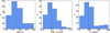 |
Fig. 1 Histograms of the selected clusters’ age, reddening, and member number. Those parameters are from the OCSN catalog of Qin23. The dashed black lines represent the median values. |
2 Sample and method
2.1 Sample
Open clusters are generally considered simple stellar populations, and all members in a cluster are supposed to present an isochrone distribution on the CMD. However, differential reddening and observational uncertainty would make the isochrone distribution become broader, leading to uncertainties when estimating the atmospheric parameters of members on the CMD. To reduce the effect of these factors, we selected open clusters with E(B − V) ≤ 0.3 from the OCSN catalog of Qin23, and then visually excluded clusters with an extended main sequence. A sample of 130 open clusters was selected, including 34 424 member stars in Gaia DR3. Fig. 1 shows histograms of the age, reddening, and number of selected clusters provided by Qin23. The logarithm ages of these clusters (log (t[yr])) are between 7 and 9; most are young. The number of members of each cluster ranges from 46 to 1986, with an average value of 269.
It is noted that Qin23 set the cut on the renormalized unit weight error as <1.4 (Lindegren 2018) to exclude sources with unreliable astrometric and photometric observations. Meanwhile, Riello et al. (2021b) introduced the corrected flux excess factor of the BP and RP flux, C*, defined as
 (1)
(1)
where C = (IBP + IRP)/IG is the BP and RP flux excess factor, and f(BP − RP) is a function indicating the expected excess at a given color for sources with high-quality photometry (Riello et al. 2021b). We used |C*|< N σC* to remove sources with inconsistent G-band photometry and BP and RP photometric measurements, where N=3, σC* in bins of 0.01 mag and fit with a simple power law in G magnitude (equation (18) in Riello et al. 2021b). Furthermore, we made use of the best isochrones fit by Qin23 for all the clusters to derive their binary sequences with a mass ratio (q) of 0.5. Subsequently, we excluded those members that have a mass ratio greater than 0.5 (q > 0.5), as is represented by the blue dots in Fig. 2. 32% of the member samples were removed in this step.
To validate the atmospheric parameters from spectroscopic surveys, we cross-matched the remaining cluster members with Gaia DR3 (GSP-Phot, GSP-Spec, ESP-HS), LAMOST-LRS DR11, APOGEE DR17, and GALAH DR4 atmospheric parameter catalogs. The atmospheric properties of the common samples are listed in Table 1. Additionally, for the GSP-Spec sample, we applied the quality flags where vbroadT, vbroadG, VbroadM, vradT, vradG, and vradM were equal to 0; that is, f1, f2, f3, f4, f5, and f6=0 in the corresponding gspspec_flags (Recio-Blanco et al. 2023).
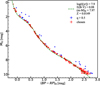 |
Fig. 2 Color-absolute magnitude diagram of OCSN 259 (Roslund 6). The dashed green line represents the best-fit isochrone provided by Qin23. The blue dots represent the members with a binary mass ratio larger than 0.5. The red dots represent the member stars we have retained. The error bars indicate the photometric uncertainties. |
2.2 Method
To evaluate the quality of the stellar parameter values in Gaia DR3, LAMOST-LRS DR11, APOGEE DR17, and GALAH DR4, we adopted members in 130 open clusters with well-defined main sequences from the OCSN catalog as standards. While we adopted the metallicity and age values of open clusters from Qin23, we acknowledge that these reference metallicities may have errors that could introduce potential biases into our analysis. For this work, we assume that these are the true values. We estimated the atmospheric parameters of member stars through the isochrone fitting approach. Then we compared the estimated parameters to those from different catalogs. The steps are listed below:
- (1)
We prepared the theoretical nonrotating isochrones for this analysis. It is important to note that the use of nonrotating models may limit the accuracy for early-type stars, particularly those of spectral types O, B, and A, where rotation plays a significant evolutionary role. Based on the cluster age and metallicity parameters provided by Qin23, we obtained the PARSEC isochrones (Marigo et al. 2017) with the Gaia photometric system (Riello et al. 2021a) from CMD 3.72 for each cluster. Furthermore, for each isochrone, we interpolated the parameters (including Giso, BPiso, RPiso, Teff_iso, log g_iso) on a mass grid with a step size of 0.0005 M⊙.
- (2)
We obtained the intrinsic color and absolute magnitude. Based on the distance modulus (m − M)0 and reddening value E(B − V) given by Qin23 for each cluster, we used AG = 2.74 × E(B − V) and E(BP − RP) = 1.339 × E(B − V) (Casagrande & VandenBerg 2018; Zhong et al. 2019) to calculate the absolute magnitude, MG = Gobs − (m − M)0 − AG, and the intrinsic color, (BP − RP)0 = (BP − RP)obs − E(BP − RP), of each member star. It should be noted that the extinction coefficient here is applicable to stars in the temperature range of [5250, 7000] K. However, it has been applied for all stars, and readers are advised to pay attention to this point (for more discussions, please refer to Sect. 4.3).
- (3)
We estimated the theoretical atmospheric parameters. On the CMD of each cluster, we matched each member to the theoretical point in the isochrone with the minimum distance. The minimum distance is defined as the minimum difference between the observed and theoretical values of
 . Then, we obtained theoretical Teff_iso and log g_iso from the isochrone for each member star. At the same time we also considered the uncertainty due to observational errors. We provide these estimated theoretical atmospheric parameters and the uncertainties in Appendix A.
 - (4)
We calculated the deviations between observational and theoretical atmospheric parameters. Adopting theoretical values as reference values, we separately calculated the differences between the crossmatched atmospheric parameters and the reference values, which are ΔTeff_surveys = Teff_surveys − Teff_iso, Δ log g_surveys = log g_surveys − log g_iso. Then, the data quality of these catalogs were evaluated.
Sample size and typical uncertainties from Gaia, LAMOST, APOGEE, and GALAH.
3 Validating atmospheric parameters
We calculated the median and dispersion values for the differences between the theoretical and observational parameters for the selected cluster member stars. Then we evaluated the atmospheric parameters provided by Gaia GSP-Phot, GSP-Spec, ESP-HS, LAMOST, APOGEE, and GALAH, and summarized them in Table 2. The crossmatched catalogs were given in Col. 1 (‘Catalogs’). Based on the deviation variations in Figs. 3 and 4, we roughly divided the member sample into different stellar type groups (Col. 2, “Stellar type”) based on the range of intrinsic colors, and calculated the corresponding median deviations (Col. 3 and 5, “Med(ΔTeff)” and “Med(Δ log g)”) and the dispersions (Cols. 4 and 6, “σ(ΔTeff)” and “σ(Δ log g)”) of stars.
Figs. 3 and 4 display the parameter deviation (ΔTeff and Δ log g) distributions for different spectroscopic surveys within different intrinsic color ranges. For the GSP-Phot sample, in the intrinsic color range of [−0.2, 3.4] mag, we calculated the median and dispersion values with a color step size of 0.1 mag. For the GSP-Spec sample, we computed the median and dispersion values in the intrinsic colors range of [0.5, 1.2] mag with a step of 0.05 mag. For the ESP-HS samples, we made similar calculations in the intrinsic color range of [−0.25, 0.3] mag with a step of 0.05 mag. For the LAMOST sample, we analyzed the parameter deviations in the intrinsic color range of [−0.2, 1.8] mag with a step of 0.2 mag. For the APOGEE sample, we evaluated the parameter deviations in the intrinsic color range of [−0.3, 2.9] mag with a step of 0.2 mag. Within the intrinsic color range of [−0.2, 3.2] mag, we performed a similar estimation for the GALAH sample with a step of 0.2 mag.
The metallicity of each catalog is also shown in Figs. 3 and 4. The metallicity of the GSP-Phot has been calibrated with the calibration relation from Andrae et al. (2023). We find that the metallicity of the B, A, and K-type stars of LAMOST-LRS DR11, GALAH DR4 seems lower than that of the G, F-type stars. In addition, there is an underestimation of the metallicity of M-type stars in GSP-Phot.
3.1 Teff, log g from GSP-Phot
Panel A in Figs. 3 and 4 presents the distribution of ΔTeff_Phot and Δ log g_Phot versus the intrinsic color. The median values for ΔTeff_Phot and Δ log g_Phot of all member stars are 101 K and −0.06 dex, respectively, while their MAD values are 232 K and 0.14 dex. It is noted that the MAD values of the difference (ΔTeff_Phot and Δ log g_Phot) in our sample are lower than those (400 K and 0.22 dex) provided by F23. Moreover, as is shown in Fig. 5 (red lines), the median dispersions of ΔTeff_Phot and Δ log g_Phot are 174 K and 0.11 dex for all the selected sample stars, which are smaller than those from Andrae et al. (2023) (see their Table 1 and Table 2). This may be because the selected comparison sample in this work is the high-quality open clusters with well-defined main sequences, and stars with a binary mass ratio larger than 0.5 were excluded. We discuss the variations of Teff and log g deviations for different types of stars in color bins, which are shown below:
- (1)
B and A-type stars: both ΔTeff_Phot and the corresponding dispersions show significant variations with a median deviation of −233 K and a median dispersion of 593 K. The median value of Δ log g_Phot and the corresponding median dispersion are −0.11 dex 0.08 dex.
- (2)
F, G, and K-type stars: ΔTeff_Phot shows a median value of −40 K and a median dispersion of 186 K. When the stellar color changed from F-type to K-type, ΔTeff_Phot gradually increased from −320 K to 150 K, which is generally in agreement with F23. The log g_Phot of the F, G, and K-type stars is mainly underestimated with a median value of −0.06 dex, and the corresponding dispersion is 0.06 dex, which is similar to the result of B23, while F23 obtained the opposite conclusion. Moreover, we found a bifurcation structure of deviations for K-type stars.
- (3)
M-type stars: the ΔTeff_Phot increases from 100 K to 350 K as the color reddens, while the dispersions are relatively stable. As M-type stars redden, the deviation of log g increases from −0.1 dex to 0.39 dex. The median values of ΔTeff_Phot and Δ log g_Phot are 213 K and 0.01 dex, and the median dispersions are 86 K and 0.16 dex.
Summary of the median values and the dispersions of ΔTeff and Δ log g in different type stars for GSP-Phot, GSP-Spec, ESP-HS, LAMOSTLRS DR11, APOGEE DR17, and GALAH DR4.
Andrae et al. (2023) point out that there is a degeneracy problem between Teff and extinction in the GSP-Phot, which means that an observed red star could be a hot star reddened owing to dust extinction on the line of sight, or a truly cool star. This makes it difficult for GSP-Phot to differentiate the two cases. Fig. 6 displays the distribution of ΔAG_Phot as a function of ΔTeff_Phot in our sample, with the color of each point representing the Δlog g_Phot. Similarly, our result shows that the Teff strongly degenerates with extinction, which may be responsible for the deviation of GSP-Phot’s atmospheric parameters from the theoretical values. The linear relation demonstrates that the temperature and extinction in the G band for most stars are simultaneously overestimated or underestimated. For stars with severely overestimated temperatures and extinctions, the GSP-Phot also overestimates their log g, and vice versa.
In addition, Fig. 7 shows the dependence of ΔTeff_Phot and Δlog g_Phot on G magnitude in the range of [6, 18] mag with a step of 0.5 mag. We found that ΔTeff_Phot varies from 240 K for fainter stars to −460 K for brighter stars, Δ log g_Phot changes from 0.14 dex to −0.16 dex as stars become brighter, and the dispersion of Δlog g_Phot is larger for the fainter stars.
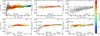 |
Fig. 3 ΔTeff vs. (BP − RP)0. The ΔTeff_Phot/Spec/HS/LAMOST/APOGEE/GALAH is defined as Teff_Phot/Spec/HS/LAMOST/APOGEE/GALAH−Teff_iso. The black triangles and error bars indicate the median values and corresponding dispersions within different color bins. The vertical dashed gray lines are the cutoffs between different stellar types. The rainbow color of the points represents the metallicity from individual catalogs with a color bar on the right. The metallicity of the GSP-Phot has been calibrated with the calibration relation from Andrae et al. (2023). Gray points refer to the samples without observational metallicity. |
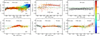 |
Fig. 4 Same as Fig. 3, but for Δlog g. The Δlog g_Phot/Spec/HS/LAMOST/APOGEE/GALAH is defined as and log g_Phot/Spec/HS/LAMOST/APOGEE/GALAH−log g_iso. |
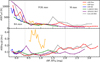 |
Fig. 5 Top panel: dispersion of ΔTeff vs. (BP − RP)0. Bottom panel: dispersion of Δlog g vs. (BP − RP)0. The red, orange, blue, green, purple, and gray lines represent the dispersion of ΔTeff and Δlog g of GSP-Phot, GSP-Spec, ESP-HS, LAMOST-LRS DR11, APOGEE DR17, and GALAH DR4, respectively. |
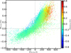 |
Fig. 6 ΔTeff_Phot vs. ΔAG_Phot. ΔAG_Phot is defined as AG_Phot − AG_iso. The color of the points represents Δlog g_Phot with a color bar on the right. |
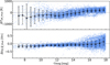 |
Fig. 7 Top panel: ΔTeff_Phot vs. Gmag. Bottom panel: Δlog g_Phot vs. Gamg. The black triangles and error bars indicate the median values and corresponding dispersions within different color bins. |
3.2 Teff, log g from GSP-Spec
The common GSP-Spec sources are mainly F and G-type stars, and some K-type stars. The distributions of ΔTeff_Spec and Δlog g_Spec are shown in panel (B) of Figs. 3 and 4. For these stars, the median value of ΔTeff_Spec is 60 K, which is relatively small, while the dispersion is 202 K. The median value of Δlog g_Spec is 0.4 dex and the dispersion is 0.3 dex. We noted a clear linear relation of the Δlog g_Spec in the color range of [0.6, 1.2] mag, with a decrease from 0.6 dex to 0.3 dex. In addition, we calibrated the log g_Spec according to the polynomial provided by Recio-Blanco et al. (2023). Although this linear structure still exists after calibration, the polynomial reduces the median deviation of log g_Spec from 0.44 dex to 0.31 dex. In Fig. 5, Δlog g_Spec (orange line) shows large dispersions. The median dispersions of ΔTeff_Spec and Δlog g_Spec in our work are larger than those in Recio-Blanco et al. (2023), because they employed a strict data quality control. In their sample, they selected the samples where the first 13 quality flags of gspspec_flags are all equal to 0, while in our sample, only the first six of these flags are equal to 0.
3.3 Teff, log g from ESP-HS
It should be pointed out that solar metallicity was assumed for all the sources in the ESP-HS module (F23). Most selected ESP-HS sources are B and A-type stars, and the distributions of ΔTeff_HS and Δlog g_Hs versus intrinsic color are shown in panel C of Fig. 3 and 4. The median value of ΔTeff_HS is −653 K. There is a clear decrease in the underestimation of Teff_HS from B-type to A-type stars, from 1450 K to 137 K. Meanwhile, the ΔTeff_HS dispersion of B-type stars is generally larger than that of A-type stars. ESP-HS underestimates the log g_HS with a relatively stable deviation of −0.2 dex and a dispersion of 0.1 dex. Fig. 5 displays the parameter dispersion distribution (blue lines). The dispersion of ΔTeff_HS in this work is similar to the result of F23. But the dispersions of ΔTeff_Hs are smaller than those in F23, with a dispersion of 0.2 dex for A-type stars to 0.4 dex for O-type stars.
3.4 Teff, log g from LAMOST-LRS DR11
As is shown in panel D of Figs. 3 and 4, the common member stars with LAMSOT-LRS DR11 are mainly F, G, and K-type stars and a few B and A-type stars. Both ΔTeff_lamost and Δlog g_LAMOST show an increasing trend from B-type to G-type stars, followed by a minor decline from G-type to K-type stars. The median ΔTeff_LAMOST and Δlog g_LAMOST are −85 K and −0.09 dex for F, G, and K-type stars. The corresponding median dispersions are of 157 K and 0.09 dex. The deviations are more significant for B and A-type stars with a median value of −579 K in ΔTeff_LAMOST and −0.37 dex in Δlog g_LAMOST, respectively. The corresponding median dispersions are 371 K and 0.08 dex. As is shown in Fig. 5 (green lines), the ΔTeff_lamost dispersion decreases as stars become redder, and the Δlog g_LAMOST dispersions are smaller than 0.15 dex with minimal variation.
3.5 Teff, log g from APOGEE DR17
Panel E of Figs. 3 and 4 shows the deviation of the Teff, log g of APOGEE DR17 from the theoretical parameters, respectively. The ΔTeff_apogee increases as stars get redder in the color range of [−0.2, 2.0] mag, from the median ΔTeff_APOGEE of −942 K for B and A-type stars to −101 K for F, G, and K-type stars. For M-type stars, we determined a median ΔTeff_apogee offset of 145 K with corresponding median dispersions of 57 K. We also found a median Δlog g_APOGEE offset −0.06 dex of for late F, G, K, and M-type stars, which indicates that the observational data is quite consistent with the theoretical model. However, the Δlog g_APOGEE shows a declining trend for B and A-type stars. As is shown in Fig. 5 (purple lines), the ΔTeff_apogee dispersion decreases as stars become redder, and the Δlog g_APOGEE dispersions exhibit noticeable variation.
3.6 Teff, log g from GALAH DR4
The deviations of the atmospheric parameters of GALAH DR4 from the theoretical values are shown in panel F of Figs. 3 and 4. The ΔTeff_GALAH shows an increasing trend for F, G-type stars, a decline feature for K-type stars, and then an increasing trend for M-type stars. We can see a Δlog g_GALAH offset of −0.05 dex for F and G-type stars and an increasing trend for K and M-type stars. Due to the limited sample number, both ΔTeff_GALAH and Δlog g_GALAH exhibit increasing features for B and A-type stars. As is shown in Fig. 5 (gray lines), for B, A, F, and G-type stars, the ΔTeff_GALAH dispersion decreases as stars become cooler, and the Δlog g_GALAH dispersions are smaller than 0.15 dex with slight variation. Then the dispersions of both parameters increase for K and M-type stars.
Overall, the parameter deviations and dispersions of different spectroscopic surveys exhibit different variations. For all the above surveys, the parameter deviations of F, G, and K-type stars are smaller than those of B, A, and M-type stars. Specifically, for B and A-type stars, the Teff deviations of Gaia data (including GSP-Phot and ESP-HS) are notably lower compared to other surveys. Conversely, for M-type stars, the Teff deviations of GSP-Phot are significantly higher than those observed in APOGEE and GALAH. Among F, G, and K-type stars, the Teff deviations are the largest for GALAH, followed by GSP-Phot, APOGEE, LAMOST, and finally GSP-Spec. As is shown in the top panel of Fig. 5, the ΔTeff dispersions decrease as stars become cooler for most samples, and the ΔTeff dispersions of K-type stars from GSP-Phot and GALAH are larger than the ones for the F and G-type stars. In the bottom panel of Fig. 5, we can see that the Δlog g dispersions of K and M-type stars are larger than the ones for the B, A, F, and G-type stars for most samples. However, the Δlog g dispersions of GSP-Spec samples are significantly larger than those in other surveys.
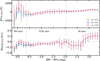 |
Fig. 8 Deviation between the Teff (upper panel) and log g (lower panel) obtained by GSP-Phot and the theoretical values of the isochrone models with different degrees of stellar rotation. The green, yellow, and red lines represent, respectively, the deviations from the theoretical isochrones with rotational angular velocities of ωi = 0.1, 0.5, and 0.9. The error bars denote the degree of dispersion in each color bin. |
4 Discussion
4.1 The influence of stellar rotation
Stellar rotation influences the atmospheric parameter derivation across all surveys. This is particularly evident in the systematic offsets observed for B and A-type stars, as has been reported consistently by multiple catalogs. We have found that the B and A-type stars of all surveys both Teff and log g are underestimated. This situation is likely associated with our failure to utilize the rotational isochrones. We employ the atmospheric parameters furnished by the rotational isochrones as a theoretical benchmark to explore how stellar rotation impacts our results.
We have selected six open clusters (OCSN_77, OCSN_90, OCSN_212, OCSN_218, OCSN_219, and OCSN_259) from our entire sample as test cases. For each cluster, we derived theoretical atmospheric parameter estimates using isochrones with specific angular rotation rates (ωi = 0.1, 0.5, 0.9). Fig. 8 presents the distribution of deviations between GSP-Phot atmospheric parameters and those derived from rotational isochrone models. Here, when we analyze the impact of rotation on GSP-Phot results, it should be understood as a case study representative of broader methodological issues affecting all datasets.
The lower panel of Fig. 8 shows that the isochrone models considering stellar rotation can reduce the degree of deviation between the log g_Phot of the B, A, and early F-type stars obtained by GSP-Phot and the theoretical values. In other words, the theoretical values of the log g_iso obtained from the isochrone models with stellar rotation are smaller than those from the isochrone models without stellar rotation. As is shown in the upper panel of Fig. 8, the theoretical values of the Teff_iso obtained from the isochrone model with stellar rotation are also smaller than that from the isochrone model without stellar rotation. We have summarized the typical deviations and dispersions of the Teff and log g of B and A-type stars under different rotational isochrones, as is shown in Table 3.
Summary of the median values and the dispersions of ΔTeff and Δlog g in B and A-type stars for GSP-Phot from different rotational isochrones models.
However, for some A-type stars, the isochrone with a much higher rotation (ωi = 0.9) will yield an even larger deviation of the Teff (as is indicated by the red line). By contrast, stellar rotation has almost no impact on late F, G, K, and M-type stars. While we use GSP-Phot as a specific example to illustrate these effects, similar discrepancies are observed across all surveys. This suggests that the source of the offsets could lie in limitations of the reference temperatures or methodologies rather than specific pipelines.
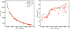 |
Fig. 9 Distribution of Teff (left) and log g (right) from GSP-Phot for the retained member stars of OCSN_259 as a function of intrinsic color. The dashed green line represents the isochrone. Red dots indicate the retained member stars. |
4.2 Dispersion at the low-mass end
The pronounced dispersion observed among low-mass stars in the CMD potentially impacts atmospheric parameter analyses across all surveys. To discuss whether the dispersion here is comparable to that of the atmospheric parameters, we presented the distribution of the observed Teff_Phot and log g_Phot of GSP-Phot with respect to the intrinsic colors for the member stars retained in Fig. 2, as is shown in Fig. 9. Consequently, the analysis of how the low-mass-end dispersion impacts GSP-Phot results also serves as a case study to illustrate the influence of the dispersion at the low-mass end that is brought to all the other survey catalogs.
For the low-mass end, such as the member stars with intrinsic colors around 2.5 mag in Fig. 2, these stars exhibit a relatively significant deviation from the isochrones and also display a relatively large dispersion. In the same color region of the left panel of Fig. 9, the Teff_Phot show a systematic overestimation, and the dispersion is not significant. However, as is shown in the right panel of Fig. 9, for the log g_Phot, there are significant deviations and dispersion in the observed values. Moreover, at the blue end of (BP − RP)0, there is also a significant underestimation and dispersion of the log g_Phot.
Although there is a relatively large dispersion in observed color and magnitude in the member stars at the low-mass end in the CMD, the observed values of their Teff_Phot exhibit a smaller dispersion. The dispersion of the observed values of the log g_Phot is significantly larger. This means that the measurement of the Teff at the low-mass end is relatively reliable, while the measurement error of the log g at the low-mass end is relatively large, showing a significant dispersion.
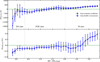 |
Fig. 10 Deviation distribution of the Teff (upper panel) and log g (lower panel) of GSP-Phot from the theoretical values obtained using different extinction laws. The dashed black and blue lines represent, respectively, the results obtained using the fixed extinction coefficient and Gaia (E)DR3 extinction law. |
4.3 The influence of the extinction law
As is well known, the extinction coefficient depends on the Teff and log g of the stars (Jordi et al. 2010). The fixed extinction coefficient we used could potentially affect all our results. To this end, we utilized the extinction law of Gaia (E)DR3 3 (Riello et al. 2021b) to calculate the extinction coefficients of member stars at different temperatures, aiming to explore the influence of different extinction coefficients on our results. We took the parameters from GSP-Phot as an example for discussion.
Consequently we applied the Gaia (E)DR3 extinction law to the member stars and recalculated the theoretical values of their atmospheric parameters, and the resulted distributions of ΔTeff_Phot and Δ log g_Phot are shown as the dashed blue lines in Fig. 10. Compared with using a fixed extinction coefficient (dashed black line in Fig. 10), for B and A-type stars, the ΔTeff_Phot using the Gaia (E)DR3 extinction law is more severely underestimated. This is in fact because the theoretical Teff_iso estimated using the Gaia (E)DR3 extinction law is higher, which further causes the deviations to become larger. As for the Δlog g_Phot deviation of B-type stars, there is an improvement to some extent, but this is not significant. In addition, for F, G, K, and M-type stars, the impact is rather negligible. This further indicates that the source of the deviation between the observed values of B and A-type stars and the theoretical values could be related to the method used.
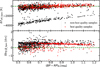 |
Fig. 11 Distribution of the deviations of Teff_Spec and log g_Spec for different quality flags in GSP-Spec. The red dots represent the highestquality samples where f1, f2, f3, f4, f5, and f6 in the gspspec_flags are all equal to 0, and the black dots represent the low-quality samples where at least one of the flags f1, f2, f3, f4, f5, and f6 is not equal to 0. |
4.4 The results of GSP-Spec with different quality flags
In Sect. 3.2, we selected the samples with the best quality in GSP-Spec by applying the condition that the quality flags of vbroadT, vbroadG, vbroadM, vradT, vradG, and vradM are all equal to 0. That is, f1, f2, f3, f4, f5, and f6=0 in the corresponding gspspec_flags. In this section, we discuss the deviation of the Teff_Spec and log g_Spec of the low-quality samples.
The black dots in Fig. 11 represent the deviation of Teff_Spec and log g_Spec of the member stars in GSP-Spec with low-quality flags, meaning that at least one of the quality flags f1, f2, f3, f4, f5, and f6 is not equal to 0. In contrast, the red dots denote the highest-quality samples. We have found that in the upper panel of Fig. 11, there is a significant underestimation of the Teff_Spec for the member stars with low-quality flags. For a portion of the low-quality sample, the deviation of Teff_Spec increases linearly from 2000 K to 4000 K. After the quality control, as is shown by red dots, this obvious linear structure of large deviation can be effectively filtered out. However, in the lower panel of Fig. 11, we found that the deviation of the log g_S pec of the highest-quality samples is nearly the same as that of the low-quality samples; both exhibit overestimating tendencies.
4.5 The limitations of our method
It is worth noting that there are still certain limitations in our work. We have used the theoretical parameters obtained from the cluster isochrones to validate the observed atmospheric parameters; however, we have not considered the fitting error of the cluster age, which may cause a certain degree of deviation in the theoretical parameters of the member stars. Although we removed binaries with a mass ratio greater than 0.5 using the binary sequence for each cluster, the low mass-ratio binaries still affect the theoretical parameter estimation. Moreover, for some clusters, the small color deviations between the observational CMDs and theoretical PARSEC isochrones exist, especially for the low-mass region (Jiang et al. 2024; Wang et al. 2024), which would impact the atmospheric assessment. In addition, the extinction coefficient we used is more applicable to the temperature range of [5250, 7000] K. For some higher-temperature stars, different extinction laws can have significant impacts on the deviation of the observed values.
The uncertainties in the PARSEC model are not considered in our work, which can be divided into two parts: physical uncertainties and computational uncertainties (Valle et al. 2013; Stancliffe et al. 2016). The physical uncertainties include nuclear reactions, radiative and conductive opacity, and mixing processes. The computational uncertainties include spatial and temporal resolutions in models, and stellar structure equation solutions. It is difficult to quantify the model uncertainties in Teff and log g, which is beyond the main goal of this article. It is important to emphasize that the isochrone models used do not include stellar rotation, which can introduce systematic offsets in the interpretation of atmospheric parameters, particularly for early-type stars.
5 Conclusions
In this paper, we selected 130 open clusters with clear and well-defined main sequences within 500 pc of our solar neighborhood to assess the quality of atmospheric parameters from large spectroscopic surveys such as Gaia, LAMOST, APOGEE, and GALAH. Meanwhile, we applied photometric quality filters and binary fraction criteria to remove sources with bad photometric observation or binary stars. Then, we estimated the theoretical atmospheric parameters for each cluster member based on the best isochrone fit by Qin23. Utilizing this unified reference library of atmospheric parameters, we evaluated the quality of atmospheric parameters from GSP-Phot, GSP-Spec, and ESP-HS of Gaia DR3, as well as LAMOST-LRS DR11, APOGEE DR17, and GALAH DR4.
Although the work of using open cluster member stars as a reference standard for atmospheric parameters and then validating the atmospheric parameters of survey data has been carried out, our sample selection is more stringent and statistically significant. By choosing a higher-quality sample of open cluster members, we are better able to assess the typical biases and dispersions of atmospheric parameters in different survey data. For example, in comparison with the work of validating atmospheric parameters by F23, it is noted that differential reddening can introduce significant biases when estimating the theoretical atmospheric parameters. Therefore, we selected clusters with clear and well-defined main sequences and removed large mass-ratio binaries (q>0.5).
Our major results include:
For B and A-type stars, there is an underestimation of Teff of these surveys, and the dispersions in B and A-type stars are all relatively large. All surveys show a significant underestimation of log g, except for the 0.01 dex of APOGEE DR17. There is a systematic offset of −0.2 dex between ESPHS and isochrone values. We need to point out that our method does not take into account the factor of rotation, which may introduce systematic effects. Moreover, the difference in extinction law may also have an impact on the results;
For F, G, and K-type stars, the Teff of the individual surveys are relatively consistent with the isochrones, and the dispersions are all within 260 K. The log g of each survey shows an underestimation, except for GSP-Spec, where there is an overestimation of 0.43 dex. GSP-Phot and APOGEE DR17 show the systematic offset of −0.08 dex and −0.05 dex compared to the isochrone values;
For M-type stars, the Teff of GSP-Phot, APOGEE DR17, and GALAH DR4 all show a relatively large positive deviation, but the dispersions are smaller, with a dispersion of 61 K being the smallest for APOGEE DR17. The log g of APOGEE DR17 has a systematic offset of −0.03 dex compared to the isochrone values, and the dispersion is also minimized at 0.09 dex.
We expect this work to serve as a valuable reference for producers and users of large-scale surveys – spectroscopic or photometric, from ground or space.
Data availability
Full Table A.1 is available at the CDS via anonymous ftp to cdsarc.cds.unistra.fr (130.79.128.5) or via https://cdsarc.cds.unistra.fr/viz-bin/cat/J/A+A/698/A295
Acknowledgements
We express our gratitude to the anonymous referee for their valuable comments and suggestions, which are very helpful in improving our manuscript. This work is supported by the National Natural Science Foundation of China (NSFC) through grants 12090040, 12090042. Jing Zhong would like to acknowledge the science research grants from the China Manned Space Project with NO. CMS-CSST-2025-A19, the Youth Innovation Promotion Association CAS, the Science and Technology Commission of Shanghai Municipality (Grant No. 22dz1202400), and Sponsored by the Program of Shanghai Academic/Technology Research Leader. Li Chen acknowledges the science research grants from the China Manned Space Project with NO. CMS-CSST-2021-A08. Songmei Qin acknowledges the financial support provided by the China Scholarship Council program (Grant No. 202304910547). This work has made use of data from the European Space Agency (ESA) mission Gaia (https://www.cosmos.esa.int/gaia), processed by the Gaia Data Processing and Analysis Consortium (DPAC, https://www.cosmos.esa.int/web/gaia/dpac/consortium). Funding for the DPAC has been provided by national institutions, in particular, the institutions participating in the Gaia Multilateral Agreement.
Appendix A Reference atmospheric parameters catalog
We provide the catalog with atmospheric parameters of the member stars used for reference. A complete list of these stars is available at the CDS, and the description of the catalog is shown in Table. A.1. Columns (1) – (10) list fundamental information about the member stars, including the Name of the cluster to which it belongs (Name), Gaia DR3 source identifier (gaia_source_id), the position coordinate in ICRS (RAdeg, DEdeg), and the G, BP, and RP magnitude and their errors in Gaia DR3. Columns (11) – (14) list the atmospheric parameters (Teff_iso, log g_iso) we estimated by matching the isochrones, and the corresponding uncertainty (e_Teff_iso, e_log g_iso). Column (15) list the minimum difference between the observed and theoretical values of  . A positive value indicates that the member star is on the right side of the isochrone, while a negative value indicates that it is on the left side.
We sampled 50 repetitions of the normality of Gmag ∼ N (Gmag, Gmag_err2) and (BP – RP) ∼ N for each member star, and used the standard deviation of the atmospheric parameters obtained from these samples as the uncertainty (e_Teff_iso, e_log g_iso). It is important to note that our estimates of uncertainties are underestimated. This is because our estimation is only based on the observations’ uncertainties, and we do not consider the uncertainties due to age, and stellar evolution models.
Description of the catalog of the member stars we used.
References
- Abdurro’uf, Accetta, K., Aerts, C., et al. 2022, ApJS, 259, 35 [NASA ADS] [CrossRef] [Google Scholar]
- Andrae, R., Fouesneau, M., Sordo, R., et al. 2023, A&A, 674, A27 [CrossRef] [EDP Sciences] [Google Scholar]
- Blanco-Cuaresma, S., Soubiran, C., Heiter, U., & Jofré, P., 2014, A&A, 569, A111 [CrossRef] [EDP Sciences] [Google Scholar]
- Bossini, D., Vallenari, A., Bragaglia, A., et al. 2019, A&A, 623, A108 [NASA ADS] [CrossRef] [EDP Sciences] [Google Scholar]
- Brandner, W., Calissendorff, P., & Kopytova, T., 2023, A&A, 677, A162 [NASA ADS] [CrossRef] [EDP Sciences] [Google Scholar]
- Buder, S., Sharma, S., Kos, J., et al. 2021, MNRAS, 506, 150 [NASA ADS] [CrossRef] [Google Scholar]
- Buder, S., Kos, J., Wang, E. X., et al. 2024, arXiv e-prints [arXiv:2409.19858] [Google Scholar]
- Cantat-Gaudin, T., Jordi, C., Vallenari, A., et al. 2018, A&A, 618, A93 [NASA ADS] [CrossRef] [EDP Sciences] [Google Scholar]
- Cantat-Gaudin, T., Anders, F., Castro-Ginard, A., et al. 2020, A&A, 640, A1 [NASA ADS] [CrossRef] [EDP Sciences] [Google Scholar]
- Casagrande, L., & VandenBerg, D. A., 2018, MNRAS, 479, L102 [NASA ADS] [CrossRef] [Google Scholar]
- Castro-Ginard, A., Jordi, C., Luri, X., et al. 2020, A&A, 635, A45 [NASA ADS] [CrossRef] [EDP Sciences] [Google Scholar]
- Castro-Ginard, A., Jordi, C., Luri, X., et al. 2022, A&A, 661, A118 [NASA ADS] [CrossRef] [EDP Sciences] [Google Scholar]
- Creevey, O. L., Sordo, R., Pailler, F., et al. 2023, A&A, 674, A26 [NASA ADS] [CrossRef] [EDP Sciences] [Google Scholar]
- Cui, X.-Q., Zhao, Y.-H., Chu, Y.-Q., et al. 2012, Res. Astron. Astrophys., 12, 1197 [Google Scholar]
- De Angeli, F., Weiler, M., Montegriffo, P., et al. 2023, A&A, 674, A2 [NASA ADS] [CrossRef] [EDP Sciences] [Google Scholar]
- Fouesneau, M., Frémat, Y., Andrae, R., et al. 2023, A&A, 674, A28 [NASA ADS] [CrossRef] [EDP Sciences] [Google Scholar]
- Fu, X., Bragaglia, A., Liu, C., et al. 2022, A&A, 668, A4 [NASA ADS] [CrossRef] [EDP Sciences] [Google Scholar]
- Gaia Collaboration (Prusti, T., et al.) 2016, A&A, 595, A1 [NASA ADS] [CrossRef] [EDP Sciences] [Google Scholar]
- Gaia Collaboration (Vallenari, A., et al.), 2023, A&A, 674, A1 [NASA ADS] [CrossRef] [EDP Sciences] [Google Scholar]
- García Pérez, A. E., Allende Prieto, C., Holtzman, J. A.,, et al. 2016, AJ, 151, 144 [Google Scholar]
- He, Z., Li, C., Zhong, J., et al. 2022a, ApJS, 260, 8 [NASA ADS] [CrossRef] [Google Scholar]
- He, Z., Wang, K., Luo, Y., et al. 2022b, ApJS, 262, 7 [NASA ADS] [CrossRef] [Google Scholar]
- Hunt, E. L., & Reffert, S., 2021, A&A, 646, A104 [NASA ADS] [CrossRef] [EDP Sciences] [Google Scholar]
- Hunt, E. L., & Reffert, S., 2023, A&A, 673, A114 [NASA ADS] [CrossRef] [EDP Sciences] [Google Scholar]
- Jiang, Y., Zhong, J., Qin, S., et al. 2024, ApJ, 971, 71 [NASA ADS] [CrossRef] [Google Scholar]
- Jordi, C., Gebran, M., Carrasco, J. M., et al. 2010, A&A, 523, A48 [NASA ADS] [CrossRef] [EDP Sciences] [Google Scholar]
- Krone-Martins, A., & Moitinho, A., 2014, A&A, 561, A57 [NASA ADS] [CrossRef] [EDP Sciences] [Google Scholar]
- Lada, C. J., & Lada, E. A., 2003, ARA&A, 41, 57 [Google Scholar]
- Lindegren, L., 2018, Gaia technical note, gAIA-C3-TN-LU-LL-124 [Google Scholar]
- Liu, L., & Pang, X., 2019, ApJS, 245, 32 [NASA ADS] [CrossRef] [Google Scholar]
- Majewski, S. R., Schiavon, R. P., Frinchaboy, P. M., et al. 2017, AJ, 154, 94 [NASA ADS] [CrossRef] [Google Scholar]
- Marigo, P., Girardi, L., Bressan, A., et al. 2017, ApJ, 835, 77 [Google Scholar]
- McInnes, L., Healy, J., & Astels, S., 2017, J. Open Source Softw., 2, 205 [Google Scholar]
- Monteiro, H., Dias, W. S., & Caetano, T. C., 2010, A&A, 516, A2 [NASA ADS] [CrossRef] [EDP Sciences] [Google Scholar]
- Netopil, M., Oralhan, I. A., Çakmak, H., Michel, R., & Karataş, Y., 2022, MNRAS, 509, 421 [Google Scholar]
- Pera, M. S., Perren, G. I., Moitinho, A., Navone, H. D., & Vazquez, R. A., 2021, A&A, 650, A109 [NASA ADS] [CrossRef] [EDP Sciences] [Google Scholar]
- Portegies Zwart, S. F., McMillan, S. L. W., & Gieles, M., 2010, ARA&A, 48, 431 [NASA ADS] [CrossRef] [Google Scholar]
- Qin, S.-M., Li, J., Chen, L., & Zhong, J., 2021, Res. Astron. Astrophys., 21, 045 [Google Scholar]
- Qin, S., Zhong, J., Tang, T., & Chen, L., 2023, ApJS, 265, 12 [NASA ADS] [CrossRef] [Google Scholar]
- Recio-Blanco, A., de Laverny, P., Palicio, P. A., et al. 2023, A&A, 674, A29 [NASA ADS] [CrossRef] [EDP Sciences] [Google Scholar]
- Riello, M., de Angeli, F., Evans, D. W., et al. 2021a, VizieR Online Data Catalog: J/A+A/649/A3 [Google Scholar]
- Riello, M., De Angeli, F., Evans, D. W., et al. 2021b, A&A, 649, A3 [NASA ADS] [CrossRef] [EDP Sciences] [Google Scholar]
- Sim, G., Lee, S. H., Ann, H. B., & Kim, S., 2019, J. Korean Astron. Soc., 52, 145 [Google Scholar]
- Stancliffe, R. J., Fossati, L., Passy, J. C., & Schneider, F. R. N., 2016, A&A, 586, A119 [NASA ADS] [CrossRef] [EDP Sciences] [Google Scholar]
- Valenti, J. A., & Piskunov, N., 2012, SME: Spectroscopy Made Easy, Astrophysics Source Code Library [record ascl:1202.013] [Google Scholar]
- Valle, G., Dell’Omodarme, M., Prada Moroni, P. G., & Degl’Innocenti, S., 2013, A&A, 549, A50 [CrossRef] [EDP Sciences] [Google Scholar]
- Wang, F., Fang, M., Fu, X., et al. 2024, arXiv e-prints [arXiv:2411.12987] [Google Scholar]
- Wu, Y., Luo, A. L., Li, H.-N.,, et al. 2011, Res. Astron. Astrophys., 11, 924 [Google Scholar]
- Zhao, G., Zhao, Y.-H., Chu, Y.-Q., Jing, Y.-P., & Deng, L.-C., 2012, Res. Astron. Astrophys., 12, 723 [Google Scholar]
- Zhong, J., Chen, L., Kouwenhoven, M. B. N., et al. 2019, A&A, 624, A34 [NASA ADS] [CrossRef] [EDP Sciences] [Google Scholar]
- Zhong, J., Chen, L., Wu, D., et al. 2020, A&A, 640, A127 [NASA ADS] [CrossRef] [EDP Sciences] [Google Scholar]
All Tables
Summary of the median values and the dispersions of ΔTeff and Δ log g in different type stars for GSP-Phot, GSP-Spec, ESP-HS, LAMOSTLRS DR11, APOGEE DR17, and GALAH DR4.
Summary of the median values and the dispersions of ΔTeff and Δlog g in B and A-type stars for GSP-Phot from different rotational isochrones models.
All Figures
|
Fig. 1 Histograms of the selected clusters’ age, reddening, and member number. Those parameters are from the OCSN catalog of Qin23. The dashed black lines represent the median values. |
| In the text | |
|
Fig. 2 Color-absolute magnitude diagram of OCSN 259 (Roslund 6). The dashed green line represents the best-fit isochrone provided by Qin23. The blue dots represent the members with a binary mass ratio larger than 0.5. The red dots represent the member stars we have retained. The error bars indicate the photometric uncertainties. |
| In the text | |
|
Fig. 3 ΔTeff vs. (BP − RP)0. The ΔTeff_Phot/Spec/HS/LAMOST/APOGEE/GALAH is defined as Teff_Phot/Spec/HS/LAMOST/APOGEE/GALAH−Teff_iso. The black triangles and error bars indicate the median values and corresponding dispersions within different color bins. The vertical dashed gray lines are the cutoffs between different stellar types. The rainbow color of the points represents the metallicity from individual catalogs with a color bar on the right. The metallicity of the GSP-Phot has been calibrated with the calibration relation from Andrae et al. (2023). Gray points refer to the samples without observational metallicity. |
| In the text | |
|
Fig. 4 Same as Fig. 3, but for Δlog g. The Δlog g_Phot/Spec/HS/LAMOST/APOGEE/GALAH is defined as and log g_Phot/Spec/HS/LAMOST/APOGEE/GALAH−log g_iso. |
| In the text | |
|
Fig. 5 Top panel: dispersion of ΔTeff vs. (BP − RP)0. Bottom panel: dispersion of Δlog g vs. (BP − RP)0. The red, orange, blue, green, purple, and gray lines represent the dispersion of ΔTeff and Δlog g of GSP-Phot, GSP-Spec, ESP-HS, LAMOST-LRS DR11, APOGEE DR17, and GALAH DR4, respectively. |
| In the text | |
|
Fig. 6 ΔTeff_Phot vs. ΔAG_Phot. ΔAG_Phot is defined as AG_Phot − AG_iso. The color of the points represents Δlog g_Phot with a color bar on the right. |
| In the text | |
|
Fig. 7 Top panel: ΔTeff_Phot vs. Gmag. Bottom panel: Δlog g_Phot vs. Gamg. The black triangles and error bars indicate the median values and corresponding dispersions within different color bins. |
| In the text | |
|
Fig. 8 Deviation between the Teff (upper panel) and log g (lower panel) obtained by GSP-Phot and the theoretical values of the isochrone models with different degrees of stellar rotation. The green, yellow, and red lines represent, respectively, the deviations from the theoretical isochrones with rotational angular velocities of ωi = 0.1, 0.5, and 0.9. The error bars denote the degree of dispersion in each color bin. |
| In the text | |
|
Fig. 9 Distribution of Teff (left) and log g (right) from GSP-Phot for the retained member stars of OCSN_259 as a function of intrinsic color. The dashed green line represents the isochrone. Red dots indicate the retained member stars. |
| In the text | |
|
Fig. 10 Deviation distribution of the Teff (upper panel) and log g (lower panel) of GSP-Phot from the theoretical values obtained using different extinction laws. The dashed black and blue lines represent, respectively, the results obtained using the fixed extinction coefficient and Gaia (E)DR3 extinction law. |
| In the text | |
|
Fig. 11 Distribution of the deviations of Teff_Spec and log g_Spec for different quality flags in GSP-Spec. The red dots represent the highestquality samples where f1, f2, f3, f4, f5, and f6 in the gspspec_flags are all equal to 0, and the black dots represent the low-quality samples where at least one of the flags f1, f2, f3, f4, f5, and f6 is not equal to 0. |
| In the text | |
Current usage metrics show cumulative count of Article Views (full-text article views including HTML views, PDF and ePub downloads, according to the available data) and Abstracts Views on Vision4Press platform.
Data correspond to usage on the plateform after 2015. The current usage metrics is available 48-96 hours after online publication and is updated daily on week days.
Initial download of the metrics may take a while.