| Issue |
A&A
Volume 697, May 2025
|
|
|---|---|---|
| Article Number | A215 | |
| Number of page(s) | 22 | |
| Section | Galactic structure, stellar clusters and populations | |
| DOI | https://doi.org/10.1051/0004-6361/202553776 | |
| Published online | 21 May 2025 | |
Searching for exotic object companions in the dense core of NGC 362
A multi-wavelength and multi-epoch photometric analysis
1
Department of Physics and Astronomy “Augusto Righi”, University of Bologna,
Via Gobetti 93/2,
40129
Bologna,
Italy
2
INAF – Astrophysics and Space Science Observatory of Bologna,
Via Gobetti 93/3,
40129
Bologna,
Italy
3
Department of Physics, University of Alberta,
Edmonton,
AB
T6G 2G7,
Canada
4
Astrophysics Research Institute, Liverpool John Moores University,
146 Brownlow Hill,
Liverpool
L3 5RF,
UK
5
INAF-Osservatorio Astronomico di Padova,
Via dell’Osservatorio 5,
35122
Padova,
Italy
6
Department of Astronomy, Indiana University,
727 E. Third St.,
Bloomington,
IN
47405,
USA
7
Institut für Astrophysik, Georg-August-Universität Göttingen,
Friedrich-Hund-Platz 1,
37077
Göttingen,
Germany
★ Corresponding author: This email address is being protected from spambots. You need JavaScript enabled to view it.
Received:
16
January
2025
Accepted:
28
March
2025
Abstract
The dense cores of globular clusters (GCs) are efficient environments for the production of exotic stellar populations, including millisecond pulsars (MSPs), low-mass X-ray binaries (LMXBs), and cataclysmic variables (CVs). Most of these objects likely form through two- and three-body interactions and are useful tracers of the cluster’s dynamical evolution. In this work, we explore the exotic object population in the galactic GC NGC 362, searching for the optical counterpart of 33 X-ray sources identified within 1′ from the cluster centre. To this end, we exploited a large Hubble Space Telescope dataset obtained in eight different epochs and covering a wavelength range from the near UV to the optical I band. To identify the most promising counterparts, we followed a multi-step analysis based on four main ingredients, namely, positional coincidence, position in the colour–magnitude diagrams, Hα excess, and photometric variability. In addition, we complemented the photometric analysis with spectroscopic information coming from the analysis of MUSE radial velocity curves. Thanks to this multi-diagnostic approach, we were able to identify 28 high-confidence optical counterparts, including several candidate MSPs, active binaries, and CVs. The most intriguing counterparts include a candidate black widow system, an eclipsing binary blue straggler, and a system in outburst, potentially representing either an LMXB or a nova eruption from a CV. The candidate MSPs proposed in this work will contribute to ongoing radio analyses with MeerKAT for the identification and detailed study of MSPs in NGC 362.
Key words: binaries: eclipsing / stars: evolution / pulsars: general / X-rays: binaries / globular clusters: individual: NGC 362
© The Authors 2025
 Open Access article, published by EDP Sciences, under the terms of the Creative Commons Attribution License (https://creativecommons.org/licenses/by/4.0), which permits unrestricted use, distribution, and reproduction in any medium, provided the original work is properly cited.
This article is published in open access under the Subscribe to Open model. This email address is being protected from spambots. You need JavaScript enabled to view it. to support open access publication.
1 Introduction
It is well established that frequent stellar dynamical interactions in the high-density cores of globular clusters (GCs) make them efficient factories for the formation of exotic objects, including millisecond pulsars (MSPs), low-mass X-ray binaries (LMXBs), and cataclysmic variables (CVs) (Paresce et al. 1992; Bailyn 1995; Bellazzini et al. 1995; Ferraro et al. 2001; Pooley & Hut 2006; Freire et al. 2008). Most of these objects are believed to result from the evolution of binary systems (Ivanova et al. 2006). Their existence is therefore closely tied to the dynamics of the parent cluster, thus making them useful indicators for tracing its dynamical evolution (Ferraro et al. 2009, 2012; Dalessandro et al. 2008b,a; Lanzoni et al. 2016; Kızıltan et al. 2017; Dickson et al. 2024). Moreover, these objects are responsible for most of the X-ray emission detected in GCs (Clark 1975; Hertz & Grindlay 1983).
Low-mass X-ray binaries are binary systems in which a neutron star (NS) or a black hole (BH) accretes mass via Roche-lobe overflow from a low-mass companion star through the formation of an accretion disc. When accretion onto the NS is low or non-existent, these systems are classified as quiescent LMXBs (qLMXBs). The latter are usually the brightest X-ray sources in the 0.5−2.5 keV band, with LX ≳ 1032 erg/s, and they show soft blackbody-like spectra (Heinke et al. 2003; Verbunt et al. 2008). Interestingly, LMXBs have long been considered the progenitors of MSPs, as mass accretion from the evolving companion eventually spins up the NS to millisecond periods (Ferraro et al. 2015). The number of MSPs per unit mass in Galactic GCs is about 103 times larger than in the Galactic field (Hui et al. 2010; Turk & Lorimer 2013; Zhao & Heinke 2022). This is due to the fact that dynamical interactions in the dense cluster cores can promote the formation of binaries suitable for recycling NSs into MSPs. This recycling phase can last up to approximately 1 Gyr and ultimately produces a rapidly spinning MSP with spin periods typically shorter than 10 ms. The companion star becomes a low-mass white dwarf (WD) with an He core or, more rarely, with a CO core (e.g. Tauris & Savonije 1999). Alternatively, another class of MSPs exists in which the companions are low-mass non-degenerate stars, the so-called spiders (Roberts 2013).
These spiders are divided into two main classes, black widows (BWs) and redbacks (RBs). The distinction between the two types of spiders lies in the mass of their companion stars. The RBs have companions with masses ranging from 0.1–0.5 M⊙, whereas BWs have companions with masses smaller than 0.1 M⊙. The evolutionary scenario of such systems is still under debate. According to the simulations performed by Chen et al. (2013), the strong MSP wind may be the discriminant factor in the evolution of the pulsar (PSR) companion into an RB or a BW, suggesting that they are the result of two different evolutionary paths. A strong evaporation scenario was also adopted by Smedley et al. (2015). On the other side, adopting an irradiation feedback scenario (Benvenuto et al. 2015; De Vito et al. 2020), Benvenuto et al. (2014) suggests that the RBs may either evolve into BWs or into canonical MSPs with an He WD companion. The connection between LMXBs and MSPs was confirmed by the discovery of a new class of binary systems known as transitional MSPs (tMSPs), which alternate between a purely accretion-powered state and a purely rotation-powered state, where they appear as RBs (Papitto et al. 2013; Pallanca et al. 2013; de Martino et al. 2015; Archibald et al. 2009).
In addition to their radio emission, MSPs also show X-ray emission (Saito et al. 1997; Verbunt et al. 1996; Zavlin et al. 2002). The majority of MSPs appear as soft thermal X-ray sources, where the emission is mostly dominated by thermal blackbody from the heated polar caps of the NS (Bogdanov et al. 2006). However, some MSPs may show sharp X-ray pulsations, which are indicative of non-thermal processes occurring in the system, as magnetospheric emission (Chatterjee et al. 2007) or non-thermal shock radiation resulting from the collision between the pulsar wind and the stellar wind (Wadiasingh et al. 2017). Notably, MSPs with degenerate counterparts typically do not show strong Hα emission because accretion is inhibited by their strong magnetic fields. In contrast, those with non-degenerate companions (spiders) may show strong Hα emission (e.g. the RB system PSR J1740-5340A in NGC 6397; Ferraro et al. 2001). This is particularly true for tMSPs, which can have accretion discs, as found for the two tMSPs PSR J1824-2452I in M28 (Pallanca et al. 2013) and PSR J1023+0038 found in the Galactic field (Bond et al. 2002; Archibald et al. 2009).
Cataclismic variables are binary systems where a WD accretes material from a secondary companion star, either a main sequence (MS) star or a sub-giant, through Roche-lobe overflow. These systems are important for searching for progenitors of type Ia supernovae, as all type Ia supernova progenitor populations are believed to be closely related to CVs, and some CVs might themselves be progenitors of type Ia supernovae (Knigge 2012). These objects exhibit hard X-ray spectra generated by thermal emission from hot plasma (Heinke et al. 2005). Identifying CVs in GCs by using X-ray positions to search for Hubble Space Telescope (HST) counterparts has been highly successful (Cool et al. 1995; Pooley et al. 2002; Edmonds et al. 2003; Cohn et al. 2010). The photometric identification of a star in an X-ray error circle as a CV has typically relied on using some combination of blue colours, variability, and/or Hα emission. All three of these signatures are produced by hot, variable, and often optically thin accretion discs produced by mass transfer. In particular, in the case of a magnetically weak CV, the line emission may originate from the optically thin regions of the accretion disc, whereas for a magnetic CV, it may come from the accretion stream (Witham et al. 2006).
Finally, active binaries (ABs) are also known to contribute to the X-ray emission observed from GCs. In these systems, the emission is due to the coronal activity of MS, giant, or sub-giant stars, where the magnetic corona contains plasma at temperatures exceeding 106 K (Güdel 2004). Examples of these systems include sub-subgiants (SSGs), red straggler stars (RSSs), BY Dra binaries, and RS CVn binaries. In optical colour-magnitude diagrams (CMDs), SSGs are observed below and redwards of the sub-giant branch, while RSSs are observed to the red of the normal red giant branch (RGB; Geller et al. 2017). The RS CVn binaries involve at least one evolved star showing enhanced coronal activity, while BY Dra binaries include two main-sequence stars where the enhanced activity is due to the tidal locking of a close binary producing fast rotation, which increases coronal activity (Dempsey et al. 1997). These systems represent the faintest X-ray sources in GCs and are often characterised by soft X-ray spectra (Verbunt et al. 2008). In the sample studied by Geller et al. (2017), 58% of the SSGs are characterised by X-ray emission with 0.5−2.5 keV luminosities of the order 1030−1031 erg/s, and 33% of them are Hα emitters. In fact, the chromospheric activity in ABs also leads to the presence of Hα emission. However, the intensity of this emission is significantly lower in ABs compared to CVs and LMXBs due to the different physical processes giving rise to it (see for example the results found in 47 Tucanae by Beccari et al. 2014).
Identifying optical counterparts to exotic objects is essential for understanding their formation and characterising their properties in terms of both their degenerate and non-degenerate components. In particular, it has been shown that the adoption of a multi-wavelength approach including X-ray and optical observations is extremely effective at characterising the properties and nature of exotic objects (Cadelano et al. 2019, 2020; Zhang et al. 2023). In fact, each of these observational methods offers unique and complementary insights into the same system, thus allowing for a more comprehensive understanding of its nature. On one side, X-ray observations provide insights into the possible presence of a compact object as well as any ongoing accretion processes or coronal activity, while the optical emission is dominated by the companion non-degenerate star.
In this framework, we explore the exotic object population in the Galactic massive GC NGC 362. This cluster is located at a distance of 8.8 kpc, it has an estimated age of 11.5 Gyr (Dotter et al. 2010; Aguado-Agelet et al. 2025), and its metallicity is [Fe/H] ∼ −1.1 (Carretta et al. 2013; Ceccarelli et al. 2024). Its kinematic properties (Bianchini et al. 2018; Libralato et al. 2018), as well as the presence of a double blue straggler star (BSS) sequence (Dalessandro et al. 2013), suggest that NGC 362 is in a post-core-collapse state. Moreover, 12 pulsars have been identified (but not yet published) in NGC 362, mostly via the TRAPUM project using the MeerKAT radio array, with nine of them residing in binary systems1.
The starting point of our analysis is the list of 33 X-ray sources identified by Kumawat et al. (2024) within 1′ from the cluster centre using 78.8 ks of Chandra data taken in 2004. In their work, Kumawat et al. (2024) used the HST UV Globular Cluster Survey (HUGS) catalogue (Piotto et al. 2015; Nardiello et al. 2018) to search for optical counterparts to these X-ray sources. They found 15 candidate counterparts, including two background active galactic nuclei (AGNs), three SSGs, two RSS counterparts, five candidate ABs, and two objects shifting between the bluer and redder parts of the RGB. According to their results, the majority of these bright optical counterparts are likely to be powered by coronal activity.
Hubble Space Telescope observations of NGC 362 used in this work.
In this work, we expand on the search for optical counterparts to the X-ray sources in NGC 362. While Kumawat et al. (2024) identified optical counterparts by performing astrometric matching between Chandra observations and the HUGS catalogue, here we make use of a larger multi-wavelength, multi-instrument, and multi-epoch HST dataset, and we adopt a data-analysis approach specifically tailored to identify possibly faint objects in strongly crowded fields. As a result, we obtain deeper CMDs – particularly in the bluer filters, where many stars were not detected in HUGS – and we incorporate H-alpha photometric analysis and investigate photometric variability of the counterparts across individual exposures. Additionally, we use the spectroscopic information secured by the integral field spectrograph Multi Unit Spectroscopic Explorer (MUSE) at the Very Large Telescope (VLT; Bacon et al. 2010), including radial velocities (RVs). The combination of the adopted approach and extended dataset enabled a deep and comprehensive search for optical counterparts, strengthening the identification of the most likely candidates and providing useful information for the characterisation of their properties.
The paper is organised as follows: in Sect. 2, we describe the HST dataset and detail the photometric analysis, including the calibration and astrometric procedures used during the reduction process. In Sect. 3, we describe our approach for identifying the optical counterparts of the X-ray sources, including their identification in the optical CMD and the analysis of their variability and Hα emission. The results of our analysis are summarised in Sect. 4, where we highlight the most interesting counterparts we discovered. In Sect. 5, we present the insights obtained from spectroscopy, including a comparison with a recent spectroscopic study and our analysis of RV curves for a subset of the high-confidence counterparts. Finally, in Sect. 6 we compare our results with the reference work by Kumawat et al. (2024) and draw our conclusions.
2 HST observations and data analysis
The photometric dataset used in this work consists of high-resolution HST images ranging from the near-UV (F225W) to the optical I band (F814W), obtained using the ultraviolet-visible (UVIS) channel of the Wide Field Camera 3 (WFC3) and the Advanced Camera for Surveys (ACS), both with the High Resolution Channel (HRC) and Wide Field Channel (WFC). Figure 1 shows the field of view (FoV) covered by all the HST observations used in this work, while Table 1 provides detailed information about them in terms of the adopted filters, number of images and exposure time.
When searching for optical counterparts of exotic objects, two major challenges have to be faced: the faintness of the companions, such as in the case of MSPs or CVs, and the significant crowding of the dense cores of GCs where these objects are typically located. As a result, achieving high photometric accuracy and completeness at faint magnitudes in crowded regions is crucial for this kind of analysis. Thus, our approach in the photometric reduction described in the following sections is guided by these requirements.
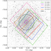 |
Fig. 1 Footprints of the FoVs covered by the HST observations listed in Table 1. The underlying stars come from the Gaia DR3 dataset (Gaia Collaboration 2023) centred on NGC 362, obtained with a search radius of 1 degree and using the Gaia G-band magnitude to scale the size of the data points. Each FoV is colour-coded according to the GO proposal number, listed in Table 1. The black cross marks the centre (RA = 15.8087453, Dec = −70.8489012, Dalessandro et al. 2013) while the black circle represents the half-mass radius, rh (63′′.5, Dalessandro et al. 2013). |
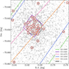 |
Fig. 2 Zoomed-in version of Fig. 1. Red circles represent the 33 X-ray sources identified by Kumawat et al. (2024). Each source is labelled with a number, following the nomenclature established by Kumawat et al. (2024). The black circle marks the core radius, rc (13′′.0, Dalessandro et al. 2013). |
2.1 WFC3 data
The WFC3 dataset consists of images obtained in two different epochs. The first contains 39 images obtained on 2012 April 13 as part of the proposal 12516 (PI: Ferraro) with the F390W, F555W, and F814W filters. The cluster core falls entirely within chip #1, and 32 out of 33 X-ray sources are located within the FoV (blue solid line in Figs. 1 and 2). The second sample contains 25 images taken on 2016 September 18, in the filters F225W and F275W as part of the proposal 14155 (PI: Kalirai). In this case the cluster core is almost entirely contained within chip #2 and all the 33 X-ray sources fall within the FoV (orange solid line in Figs. 1 and 2). In both cases, the reduction was performed on UVIS calibrated exposures that include the charge transfer efficiency (CTE) correction (_flc images). Additionally, for the F225W and F275W images, cosmic rays were removed using the Python package lacosmic (van Dokkum 2001). After correcting the frames for the “Pixel-Area-Map” (PAM), we conducted the photometric analysis using the DAOPHOT package (Stetson 1987) separately for the two datasets but following the same steps, which are described below.
As a first step, we created a list of stars using the FIND package, including only sources having peak counts larger than a given threshold above the local background level. This limit was set at 5σ for the first dataset and 3σ for the F225W and F275W images, where σ is the standard deviation of the local background noise. Using PHOTO we obtained the concentric aperture photometry of each source. For each image we selected a large number (∼200) of bright, unsaturated and isolated stars. These stars were then used to derive the best-fit point-spread function (PSF) through the package PSF. The PSF model that best reproduces the observed PSF is a Penny function (Penny 1976) for the F814W images and a Moffat function (Moffat 1969) with β = 1.5 and β = 2.5 for the F555W and F390W, F225W, F275W frames, respectively. The best-fit PSF models were then applied to all the sources using ALLSTAR. Finally, for each of the two datasets, we took full advantage of the ALLFRAME (Stetson 1994) routine to simultaneously fit stellar sources in all available images. This required the creation of a master list including all the stars that have to be fitted. Using DAOMATCH and DAOMASTER, we generated, for each filter, a list of stars with their average magnitudes and associated errors, determined from the dispersion of individual measurements. Only sources measured in at least half of the images +1 were included. The lists from the different filters were then combined into the final master list, again using DAOMATCH and DAOMASTER.
The WFC3 images are characterised by significant geometrical distortions across the FoV. Therefore, we corrected the instrumental positions of the first dataset with the equations by Bellini & Bedin (2009) for the filter F814W, while we used the coefficients of the F225W for the second dataset. We then transformed the instrumental coordinates to the absolute coordinate systems by cross-matching the WFC3 catalogue with the Gaia DR3 dataset (Gaia Collaboration 2023). Instrumental magnitudes were reported to the VEGAMAG photometric system either by using stars in common with the catalogues by Dalessandro et al. (2013), Piotto et al. (2015) and Nardiello et al. (2018) for bands in common or by applying appropriate equations and zero points for the remaining filters (which are the F225W and F435W), as reported on the HST website2 (see also Sirianni et al. 2005).
Finally, the catalogues derived from the photometric analysis of the two WFC3 datasets were cross-matched and combined, producing the final WFC3 catalogue. This comprehensive catalogue includes all stars detected in at least one band across both WFC3 observation datasets and contains over 130 000 sources.
2.2 ACS/HRC data
The WFC3 catalogue has been supplemented with additional images obtained with the ACS HRC. The HRC images used in this work were taken on 2004 December 06 as part of the proposal 10401 (PI: Chandar). This dataset comprises 16 exposures, each with texp = 85 s, in the filter F435W. These high-resolution images, despite their limited FoV, are a valuable resource for our work as they encompass a significant portion (22 out of 33) of the X-ray sources identified by Kumawat et al. (2024), as shown in Fig. 2. In fact, their inclusion is primarily motivated by the need for enhanced resolution in the cluster’s most densely populated region. Additionally, this dataset allowed us to study the variability of our counterparts over a longer temporal baseline (see Sect. 3.2).
In this analysis we employed the basic fully pipeline-calibrated individual exposures (_flt images). We processed each image using the most recent PAM images from the HST website. Following the same procedure as for the WFC3 images, we used DAOPHOT for the photometric analysis and selected approximately 100 bright isolated stars to construct the PSF model. We employed a Penny model for all frames. The PSF model was applied using ALLSTAR and ALLFRAME, and the star positions and magnitudes were then combined using DAOMATCH and DAOMASTER, requiring sources to be measured in a minimum of nine out of 16 images. We corrected for the geometrical distortions across the FoV using the equations by Meurer et al. (2003). The instrumental positions have been transformed to the absolute coordinate system using the same Gaia DR3 reference catalogue mentioned above and the instrumental magnitudes have been converted to the VEGAMAG photometric system following the guidelines and zero points provided in the ‘ACS Calibration and Zeropoints’ Web site3. The final HRC catalogue contains ∼ 11 000 sources.
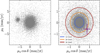 |
Fig. 3 Left: full proper motion VPD from the HSTPROMO catalogue. Right: proper motion VPD for stars within the F606W magnitude bin that includes one of the candidate counterparts of X5 (the object shown in blue in Fig. 6). The purple point indicates the object’s position in the VPD along with its associated errors. The blue, orange and red circles represent the 1σ, 2σ, and 3σ contours, respectively. |
2.3 ACS/WFC data and final catalogue construction
Finally, we include ACS/WFC photometric information, mostly from the public ACS/WFC catalogue from the ‘Hubble Space Telescope Proper Motion (HSTPROMO) Catalogs of Galactic Globular Cluster’ (Libralato et al. 2018, 2022). This includes measurements in the F606W and F814W bands, derived from images taken under proposal ID 10775 (PI: Sarajedini). Additionally, we included the mF435W, mF625W and mF658N magnitudes (from proposal ID 10005) provided by Libralato et al. (2018, 2022) via private communication. As outlined in Sect. 3.3, this allowed us to analyse the Hα emission of our candidate counterparts.
By cross-matching and combining our WFC3 and HRC catalogues with the public HSTPROMO catalogue, we constructed a comprehensive dataset containing more than 154 000 sources. This dataset includes relative proper motion measurements for stars in common between our catalogues and the HSTPROMO catalogue, which is used for investigating the cluster membership probabilities. To assess membership, we excluded stars associated with the Small Magellanic Cloud (SMC) by selecting only stars with proper motions within a 3 mas/yr radius circle centred at (μα cos δ = 0 mas/yr, μδ = 0 mas/yr) in the proper motion vector-point diagram (VPD). In fact, in addition to the cluster population centred in the VPD, the diagram reveals another subpopulation, at (μα cos δ = −6 mas/yr, μδ = 1.5 mas/yr) which corresponds to SMC stars (see the left-hand panel of Fig. 3). Subsequently, we divided the catalogue into seven bins based on F606W magnitude. We performed a 2D Gaussian fit on the VPD for each bin to determine the 1σ, 2σ, and 3σ contours. Stars falling outside the 3σ contour, even after accounting for proper motion uncertainties, were classified as non-members. An example of this analysis is shown in the right-hand panel of Fig. 3, where we highlight the position of one of the candidate counterpart of X5 (the object marked in blue in Fig. 6).
Additionally, we assigned a photometric quality flag to each star in the catalogue. For the magnitudes of the HSTPROMO catalogue, we used the diagnostic parameters described in Libralato et al. (2018), applying the same quality cuts as outlined in their Appendix B. For the WFC3/UVIS and ACS/HRC magnitudes, we identified well-measured stars performing a selection based on the CHI and SHARP photometric parameters derived for each filter by DAOPHOT. To this end, we divided our sample into ten magnitude bins, we computed the mean and performed the selection using an iterative 3σ-rejection method. An example is shown in Fig. 4 for the F814W filter. In Fig. 5, we present a sequence of (mF555W, mF390W−mF555W) CMDs illustrating the data refinement process. The first panel displays the observed CMD, including all stars of the catalogue. In the second panel, we display the CMD after removing the stars with bad photometric quality. Finally, the last, rightmost panel shows the final CMD, refined by applying photometric quality cuts and membership selection, as outlined above. The vertical sequence in the first two CMDs at (mF390W−mF555W) ∼ 0.7 is the MS of the SMC. From the cleaned diagram, it is clear that all evolutionary sequences are narrow and well-defined. A key feature of our catalogue is its depth, extending up to 8 magnitudes below the turn-off.
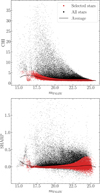 |
Fig. 4 CHI parameter (top panel) and SHARP parameter (bottom panel) as a function of mF814W magnitude. Objects in red represent selected stars following the 3σ-rejection method, while black points are rejected stars. The solid black line represents the average CHI (top panel) and average SHARP (lower panel). It can be observed that both CHI and SHARP display an irregular pattern at brighter magnitudes, particularly for mF814W < 17. This irregularity occurs due to the saturation affecting the magnitudes of these stars. Consequently, the average and standard deviation within these bins are affected, leading to the observed behaviour. |
3 Identification of optical counterparts
The primary goal of this work is to identify and characterise the optical counterparts of the 33 X-ray sources identified in NGC 362 by Kumawat et al. (2024). To this end, we followed a four-step approach that accounts for i) positional coincidence between X-ray observations and HST, ii) stellar position in the CMDs, iii) photometric variability, and iv) Hα excess.
In the following, we refer to the X-ray sources using the same names adopted by Kumawat et al. (2024), and we mark the candidate optical counterparts with a ‘c’ as a superscript. For X-ray sources with multiple candidate counterparts, we distinguish among different candidates by appending a capital letter to their names, starting from ‘A’.
3.1 Positional coincidence and CMD location
As a first step, we searched for optical counterparts for every X-ray source within the X-ray positional 95% confidence uncertainty radius (uncx) using the WFC3 catalogue. An example of a finding chart is shown in Fig. 6 for the X-ray source X5. All the other finding charts are shown in Appendix B. Then, all candidates were placed in the optical CMDs, using different filter combinations, to investigate their position. Particular attention was given to objects that displayed unusual positions, deviating from the expected evolutionary paths. Indeed, an anomalous position in the CMD could be indicative of multiple sources of light in the system or a perturbed state of the companion star. For instance, an accretion disc can shift a CV to the blue of the main sequence, or a second star can shift an AB to the red of the main sequence, while heating, mass loss, or tidal deformation can also alter the CMD position (see for example Cocozza et al. 2008; Pallanca et al. 2010).
3.2 Counterparts variability
One of the most important additions of our work is the possibility to study the variability of the optical counterparts. This is a crucial point when searching for companions of exotic objects. For example, in interacting binaries we expect photometric variability due to different processes as irradiation or tidal distortions. Moreover, in the case of MSPs, there is strong evidence confirming the optical counterpart as the companion to the MSP if the pulsar’s orbital period and ascending node time (e.g. phase), derived from radio observations, match those of the optical counterpart (e.g. Edmonds et al. 2002; Pallanca et al. 2010).
To identify variable stars, we used the Stetson variability index (J as defined by Stetson 1996). This index is computed in the photometric reduction performed with DAOPHOT and it examines the reliability of successive changes in the star’s brightness, taking into account the uncertainties associated with the measurements. Specifically, we plotted the J index as a function of magnitude for all the stars in the catalogue, for each filter. We divided the sample into ten magnitude bins, calculated the median for each bin, and obtained a list of variable stars, considering as variable those sources that were more than 2 sigma from the median in at least two filters. We then checked if any of our candidate counterparts were present in the list of all variable stars and visualised their light curves. In addition to this, we also visually inspected the light curves of all those candidate counterparts displaying unusual positions in the CMDs.
To study the variability of our sources, we used both WFC3 and HRC data. The temporal baseline spans approximately 7 hours for the F390W, F555W, and F814W images, with overlapping observation times. The F225W images cover a time range of nearly 6 hours, while the F275W frames span more than 3 hours. Also in this case, the images overlap in time. On the other side, the temporal baseline of HRC images spans 2 hours and 27 minutes. To get an estimate of the period of the flux modulation in each filter we applied the Lomb-Scargle Periodogram method (Lomb 1976; Scargle 1982) implemented in astropy (Astropy Collaboration 2013, 2018). Afterwards, we opted to merge all the available measurements, possibly broadening our temporal baseline and allowing us to capture objects with longer periods. To do so, we chose one reference magnitude and, for each available filter, we computed the shift between its average magnitude and the average reference magnitude. We thus obtained the combined global light curve and performed the Lomb-Scargle analysis on it. Moreover, we computed the False Alarm Probability (FAP) using the method described by Baluev (2008) and implemented in astropy. As an example, we plot in Fig. 7 the global light curve of one of the candidate counterparts for the X-ray source X5. This object is the one marked with a blue circle in Fig. 6, closest to the X-ray position, and is also shown in the VPD in Fig. 3. This is the light curve obtained combining all the filters of the first WFC3 dataset, taking mF555W as reference magnitude, and folding the measured data points with the period obtained from the Lomb-Scargle method. The light curve shows a very broad peak and varies within a range of over 2 magnitudes (for more details see Sect. 4.2).
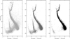 |
Fig. 5 Data selection process schematically illustrated in (mF555W, mF390W−mF555W) CMDs. The left panel shows the observed CMD, including all detected stars. The middle panel shows the cleaned CMD after photometric quality cuts. The fraction of stars removed according to photometric quality cuts is 0.53. It can be observed that the stars in the upper part of the RGB and those on the horizontal branch are excluded after the photometric quality cuts, which is a result of saturation. The right panel shows the final CMD after membership selection. The fraction of stars removed according to membership evaluation with respect to the complete catalogue shown in the first panel is 0.05. |
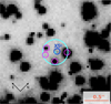 |
Fig. 6 Finding chart for source X5 in the F390W WFC3 band covering an area of 2.4′′ on each side. The cyan circle is centred on the X-ray position, indicated by a cyan cross, and it has a radius equal to the X-ray position uncertainty uncX. The magenta circles denote the positions of the candidate counterparts. We mark in blue the candidate counterpart X5c, which is the same as the one presented in Figs. 3 and 7. |
3.3 Selection of Hα emitter candidates
As mentioned previously, employing the mF658N catalogue (Libralato et al. 2018, 2022), we are able to identify the objects showing Hα excess among the X-ray candidate counterparts. In fact, when a binary system harbours a compact object, mass transfer phenomena may occur. This can generate substantial Xray and UV radiation in addition to emission lines such as Hα. Especially when we have multiple potential counterparts for an X-ray source, which is common when using positional coincidence as a selection criterion in dense environments such as the cores of GCs, the presence of Hα excess in one of them would identify it as the most likely counterpart among the candidates. For example, Beccari et al. (2014) demonstrated the effectiveness of combining broadband V and I with narrowband Hα images to detect CVs. Moreover, this method has been successfully employed in GCs, as demonstrated by Pallanca et al. (2017) in NGC 6397. For this reason, studying the Hα emission provides valuable information that we can incorporate to identify these counterparts and obtain more insights about accretion processes or coronal activity occurring in these systems.
Here we used the (mF555W−mF658N) versus (mF555W−mF814W) colour–colour diagram as diagnostic to identify Hα emitters. Before proceeding, we decided to clean the catalogue, both in terms of membership and photometric quality, following the procedure described at the end of Sect. 2.3. The main point of this analysis is that the majority of the stars in the cluster are expected to have a negligible Hα emission and they define a relatively narrow sequence in the colour–colour diagram, while the objects showing Hα emission are located above this sequence. As the influence of the Hα line on the mF555W magnitude is negligible, the Hα excess can be derived computing the distance of the object from the main sequence of the colour-colour diagram. In this work we decided to follow the same kind of approach adopted by De Marchi et al. (2010), Beccari et al. (2014) and Pallanca et al. (2013,2017). We computed the median of the (mF555W−mF658N) colour using only stars with intrinsic photometric error (defined as σmFS55W−mF658N =  ) smaller than 0.1 mag. The median defines the reference line for stars without Hα excess. For each star of the catalogue we then computed the difference between the intrinsic (mF555W−mF658N) and the value of (mF555W−mF658N) obtained projecting on the median line at the source (mF555W−mF814W). We call this difference Δ Hα. If a star shows ΔHα>5σ(mFS55W−mF658N), then it is classified as an Hα emitter. This approach allowed us to select the objects with a true colour excess and discard those with large intrinsic photometric error. Following this approach we identified 1366 candidate stars showing Hα excess out of more than 45 000 selected stars. While we acknowledge that our approach is more conservative in terms of the number of objects classified as candidate Hα emitters, it was chosen to ensure the inclusion of weak emitters, such as ABs and MSPs. A more restrictive 3σ-based method was also considered, where σ was defined as vertical width of the sequence, but this approach posed the risk of excluding such objects. The effectiveness of our method is supported by cases such as the X20c counterpart, which was spectroscopically confirmed as an Hα emitter by Göttgens et al. (2019, see Sect. 4.3).
For the selected candidate emitters, we also computed the photometric equivalent width (pEW) of the Hα emission line by adopting Eq. (4) in De Marchi et al. (2010):
![Mathematical equation: $\mathrm{pEW}=\mathrm{RW} \times\left[1-10^{(-0.4 \times \Delta \mathrm{H} \alpha)}\right],$](/articles/aa/full_html/2025/05/aa53776-25/aa53776-25-eq2.png) (1)
(1)
where RW is the rectangular width of the filter in Å units. In this context, the pEW is a very useful parameter for distinguishing between different types of objects. In Fig. 8, we plot the colour-colour diagram and we highlight in red the median line and the candidate Hα emitters. We also plot in blue the candidate counterparts showing an Hα excess (see Sect. 4.3).
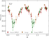 |
Fig. 7 Global light curve of one candidate counterpart to the X5 source (object marked in blue in Fig. 6) obtained by combining the data points from F390W, F555W, and F814W WFC3 images (in green, orange and red respectively). The light curve is folded with a period of 5.08 hours, obtained from the Lomb-Scargle analysis. The grey solid line, a combination of sines and cosines fitted to the data points. It has no physical meaning, it is plotted only to facilitate the visualisation of the curve. |
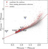 |
Fig. 8 Colour-colour diagram constructed with (mF555W−mF658N) versus (mF555W−mF814W) colours. Grey points are stars passing the photometric and membership selection. Candidate Hα emitters are represented in red. We plot in blue the candidate optical counterparts that we found to have an Hα excess (see Sect. 4.3). |
4 Results
In this section we summarise the main results obtained in our analysis. In Sect. 4.1 we present the most interesting counterparts in terms of CMD position. Section 4.2 lists the counterparts showing coherent and variable light curves, while the candidate counterparts for which we found Hα excess are presented in Sect. 4.3. As a final outcome of this analysis we build a list of ‘high-confidence’ optical counterparts to the X-ray sources in NGC 362. This sample includes stars that meet at least one of the following criteria: interesting CMD position, magnitude variability and presence of Hα excess. Additionally, in cases where only one counterpart is found within the X-ray uncertainty radius, we included it among the high-confidence counterparts.
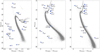 |
Fig. 9 From left to right, CMDs of (mF225W, mF225W−mF275W), (mF555W, mF390W−mF555W), and (mF555W, mF555W−mF814W). Counterparts showing peculiar CMD position are plotted in blue. Objects that become bluer in the mF390W−mF555W CMD might have an accretion disc and/or a WD. Squares indicate those counterparts that were identified also by Kumawat et al. (2024). The step observed along the RGB at mF555W ∼ 17 in the (mF555W, mF555W−mF814W) CMD is due to issues related to saturation in the F814W filter. |
4.1 Counterparts with unusual CMD position
As anticipated in Sect. 3.1, the necessary condition for an object to be considered as a candidate counterpart is that its location falls within the uncertainty radius of the X-ray position. Using our catalogue, we found at least one candidate optical counterpart for each X-ray source. When the uncertainty radius is small, we found a limited number of counterparts for a single X-ray source, while for larger uncertainty radii we found up to a maximum of 45 candidate counterparts. The final result is a list of 530 candidate counterparts for all the 33 X-ray sources, including all the 15 candidate counterparts identified by Kumawat et al. (2024). Among these 530 candidates, ten have only measurements in the F435W ACS/HRC data. Unfortunately, the lack of measurements in other filters for these ten candidates prevented their visualisation within the CMDs. Additionally, variability analysis of these candidates did not reveal any evidence of variable light curves, likely due to the limited temporal coverage of the HRC images (see Sect. 3.2). All the other candidates were placed in different CMDs in order to investigate their position within the evolutionary sequences, using different combinations of filters. In Fig. 9 we show the location of candidate counterparts falling out of the main evolutionary sequences.
Four objects (X9c, X10c, X12c, X21Ac) are located on the red side of the RGB in the (mF555W, mF555W−mF814W) CMD. However, in the (mF225W, mF225W−mF275W) and (mF555W, mF390W− mF555W) CMDs, X9c shifts towars bluer colours, indicating the possible presence of an accretion disc and/or a blue component, such as a WD. A similar behaviour is observed for X10c in the (mF225W, mF225W−mF275W) CMD. Two counterparts (X16Bc and X23c) are found in the BSS sequence. In the (mF555W, mF390W−mF555W) CMD, X23c is slightly redder than the BSS sequence, but interestingly, it becomes bluer than the bulk of BSS stars in the (mF555W, mF555W−mF814W) CMD. Following our membership evaluation, all these objects appear to be members of the cluster. In this context, the study conducted by Rozyczka et al. (2016) gives us insight into the nature of these systems. Specifically, they monitored the NGC 362 field to identify variable stars and obtained light curves for 151 periodic variable stars. Two of the most interesting objects they identified are the so-called V20 and V24. The latter coincides with our X10c, as also pointed out by Kumawat et al. (2024). The period measured for this object is 8.1 days, and the light curve suggests that this could be a semidetached binary system, formed by two ∼0.8 M⊙ stars, where the primary giant is filling its Roche lobe and the blue companion could be either a BSS or an accreting WD. It is worth mentioning that the variability of X10c (see also the case of X23c as discussed in Sect. 4.2) could account for their rather unusual colours.
X15c, X16Ac, X20c and X24Bc are located in the SSG region. All of them are classified as cluster members according to our analysis of the proper motions. Within the scope of this work, the SSG region is of particular interest, since it is a typical CMD position where exotic binaries as SSGs are often found. In general, objects located in the SSG region have experienced unusual binary evolution, such as mass transfer from a star evolving up the sub-giant branch (SGB; Leiner et al. 2017). Moreover, RB MSPs can also populate this region, as found, for example, by Ferraro et al. (2001), Cocozza et al. (2008) and Bogdanov et al. (2010); Zhang et al. (2022) for COM-6397A, COM-6266B and COM-6397B, respectively. Another example of exotic object found in this CMD region is the CV AKO 9 found in 47 Tucanae by Knigge et al. (2003).
Another interesting CMD region is the area, at faint magnitudes, between the cluster’s MS and the WD sequence. Typically, this region hosts BW systems, as in the case of COM-M5C in Pallanca et al. (2014) and COM-M71A in Cadelano et al. (2015), CVs, as CV4 and CV7 in Pallanca et al. (2017) and RBs, as 47 Tuc W found by Edmonds et al. (2002). This region also includes qLMXBs (e.g. the X5 source found in 47 Tucanae by Edmonds et al. 2002) and background galaxies with AGN (e.g. CX2 in M4; Bassa et al. 2005). In the (mF555W, mF390W−mF555W) CMD, this area contains six counterparts (X4c, X5c, X6c, X19c, X21Bc, and X24Ac). However, in the (mF555W, mF555W−mF814W) CMD, X24Ac moves towards the MS and X21Bc shows a shift towards redder colours relative to the MS. In the (mF225W, mF225W–mF275W) CMD X6c lies on the WD cooling sequence, possibly suggesting the presence of a WD in this system. On the other side, X5c is missing from the (F225W, F275W) catalogue, as it is fainter than the detection threshold reached in our photometric reduction of the second WFC3 dataset. We decided to recover its mF225W and mF275W magnitudes by combining all the images using the MONTAGE command in DAOPHOT (Stetson 1987), and performing the same photometric reduction described in Sect. 2.1 up to the ALLSTAR step on the combined images. This process allowed us to retrieve the mF225W and mF275W magnitudes for X5c and to display it in the (mF225W, mF225W−mF275W) CMD as well. Finally, there are two other stars that populate this area in the (mF225W, mF225W−mF275W) CMD. These objects are potential counterparts for the X17 and X2 X-ray sources. The X2c candidate has no measurements in the other WFC3 filters due to saturation from a nearby star, whereas X17c is more unusual, as it is missing from the other WFC3 images, as detailed further in Sect. 4.2. As for the membership, only X5c and X6c fall within the 3σ contours on their proper motion diagram when errors are considered. On the other side, X4c, X24Ac and X21Bc do not appear to be cluster members, while no proper motion information is available for X17c and X2c. The counterpart X19c, is located near the WD sequence of the (mF555W, mF390W−mF555W) CMD, while it is absent in the (mF555W, mF555W−mF814W) CMD because it lacks the mF814W magnitude. In the (mF225W, mF225W−mF275W) CMD this source shifts towards redder colours. However, we should note here that to recover the mF225W and mF275W magnitudes of X19c, we applied the same procedure used for X5c. As a consequence, the derived magnitudes may be affected by relatively large uncertainties. Also in this case no proper motion information is available.
Finally, in the (mF225W, mF225W−mF275W) CMD, the WD cooling sequence includes four objects (X18Ac, X18Bc, X25Ac and X28c). The counterpart X25Ac appears redder in the other two CMDs shown in Fig. 9. Specifically, it aligns with the MS in both the (mF555W, mF390W−mF555W) and (mF555W, mF555W−mF814W) CMDs. This behaviour could be due to the presence of an accretion disc or a blue companion, such as a WD, which becomes prominent in the UV filters. Lastly, the candidate counterpart for X28, which lies along the WD cooling sequence in the (mF225W, mF225W−mF275W) CMD, lacks mF390W and mF555W measurements due to being below the detection threshold. For the same reason, both X18Ac and X18Bc are detected only in the F225W and F275W filters. As a result, the position of these three counterparts in the other two CMDs in Fig. 9 could not be investigated. According to the VPD analysis, X25Ac and X28c are not cluster members, while no information is available for X18Ac and X18Bc. Nevertheless, the fact that these four objects align with the WD cooling sequence in the UV CMD makes them interesting candidate counterparts. For example, they could be CVs, where the UV emission is dominated by the WD.
4.2 Counterparts showing variability
As previously mentioned in Sect. 3.2, the second step of our analysis consists in studying the flux modulation of all candidate counterparts that displayed unusual positions in the CMD (see Sect. 4.1) and/or were classified as variables following our analysis of the Stetson variability index J (Stetson 1996), as detailed in Sect. 3.2.
Among all the candidates, only five4 objects display clear variability and consistent light curves across all filters: X5c, X7c, X16Bc, X23c and X33c. The light curve of X5c was shown as an example in Fig. 7, while the light curves of the other four candidate counterparts are presented in Fig. 10. We overlay a grey solid line representing a combination of sines and cosines. This line has no physical meaning; it is purely meant to facilitate the reading of the light curve. We anticipate that the FAP computed for these five sources, as detailed in Sect. 3.2, are very low, and their specific values are provided in the following paragraphs.
4.2.1 X5c
This is one of the five objects falling inside the uncertainty radius of the X5 X-ray source. It is located at only 0′′.03 from the X-ray position and it has a very blue position in the CMDs, as detailed in the previous section. As also shown in Fig. 3, the VPD suggests that X5c is a likely cluster member. The FAP for this source is 3.29 ⋅ 10−7. The light curve of this candidate counterpart is depicted in Fig. 7. In this case, we were unable to supplement the light curve with HRC data because the star is absent from the final catalogue obtained with HRC images. In fact, X5c is located right at the edge of HRC’s FoV, and due to the slight offset applied to each exposure, the source appears in fewer than half of the images, thus not fulfilling the criteria adopted during the data-reduction procedure. Additionally, individual measurements in the F225W and F275W filters are not available for this object either. As described in the previous section, retrieving the mF225W and mF275W magnitudes for X5c required photometric reduction on the combined images. As a consequence, it was not possible to obtain individual magnitudes. After aligning the three light curves to the mean mF555W magnitude and using the Lomb-Scargle periodogram method, we obtained a period of 5.08 hours, which is the period we used to fold the light curve in Fig. 7. The light curve shows a broad maximum, with an amplitude of more than 2 magnitudes. This pattern resembles typical BW light curves, known for their characteristic singular minimum and maximum structure, which is commonly attributed to the heating of the companion side exposed to the pulsar’s flux. An illustrative example is the light curve derived for the BW system PSR B1957+20 by Reynolds et al. (2007). Interestingly, the period nicely aligns with typical BW periods. The hypothesis that this object could be a BW is also supported by its position in the CMD, which resembles that of COM-M71 (Cadelano et al. 2015) and COM-M5C (Pallanca et al. 2014). An alternative hypothesis is that this could be a CV.
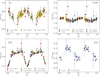 |
Fig. 10 From left to right, top to bottom: Global light curves of X7c, X16Bc, X23c, and X33c. The light curve of X7c does not show mF225w and mF275W measurements for clarity. The curves are folded using periods of 8.89 hours, 13.44 hours, 9.53 hours and 3.10 hours respectively, determined from Lomb-Scargle analysis performed on the global curves across all available filters. In each panel, the grey solid line is a combination of sines and cosines fitted to the data points with the only purpose of helping the visualisation of the light curve. |
4.2.2 X7c
This object is the only candidate for the X7 X-ray source surpassing at least one criterion for being included in our list of high-confidence counterparts. It is located in the binary sequence at mF555W ∼20 (see Fig. 16). Notably, most X-ray sources with counterparts detected in the binary sequence are thought to be coronally active binaries, or BY Dra systems (Edmonds et al. 2003; Bassa et al. 2004). No membership information is available for this source, as it is not present in the HSTPROMO catalogue (Libralato et al. 2018, 2022). The FAP of X7c amounts to 1.62 ⋅ 10−7 as X7c falls within the HRC FoV and it is retrieved in the final HRC catalogue, we had the opportunity to study its variability with HRC images. Due to the fact that the temporal baseline of HRC observations is considerably shorter compared to WFC3, we did not detect any variability using HRC alone. However, we used HRC data to complement WFC3 measurements and perform the period analysis on a much wider baseline, by shifting all the magnitudes to the mF555W one. The period derived from the global light curve is 8.89 hours, and it is used to fold the combined curve shown in the top-left panel of Fig. 10. Although the mF225W and mF275W data points were used to derive the period from the combined light curve, we chose not to display them for clarity reasons, as their larger errors compared to the other filters would make the visualisation of the light curve less clear. With an amplitude of roughly 0.2 magnitudes, the variability of X7c is less pronounced than that of X5c. However, this object is still pretty interesting, particularly considering that also exotic objects such as RB systems typically exhibit small variability amplitudes.
4.2.3 X16Bc
This is, with the SSG X16Ac, one of the two counterparts with interesting CMD position that we identified for the X-ray source. It aligns precisely with the BSS sequence across all filter combinations and it is confirmed as a cluster member based on the proper motion analysis. This object was detected both in the WFC3 and HRC images. By combining all available measurements using mF555W as the reference magnitude, we derived a period of 13.44 hours. This period was used to fold the combined light curve, shown in the top-right panel of Fig. 10. The FAP is equal to 2.66 ⋅ 10−8. As in the previous case, the light curve displays small fluctuations, within 0.1 mag. The light curve, the CMD position and the period suggest that this star might be a WUMa star, defined as a semi-detached binary system with ongoing mass transfer. Four WUMa stars were found in NGC 362 by Dalessandro et al. (2013), but X16Bc is not among these stars. However, it could be another possible candidate. Moreover, using Eq. 1 in Rucinski (2000) for the MV = MV(log P, V − I) calibration for WUMa systems, we get a fairly good agreement between the  computed from the equation using the period inferred from our analysis and the MV = 2.50 computed for X16Bc assuming E(B−V) = 0.05 (Harris 1996) and a distance of 8.8 kpc (Dotter et al. 2010). This further indicates that this system might indeed be a WUMa. Finally, WUMa stars are closely linked to X-ray emission, as noted by Heinke et al. (2005), who highlights that 11 out of 15 WUMa binaries in 47 Tucanae were detected as Chandra sources. In fact, due to their rapid rotation, with periods ranging from 0.3 to 0.6 days, WUMa stars are expected to exhibit the highest coronal activity relative to their surface area.
4.2.4 X23c
This object was already included in the list of objects showing peculiar CMD position. Indeed, in the (mF390W−mF555W) CMD, it is close to the BSS sequence but exhibits a slightly redder colour. On the other side, when plotted in a (mF555W−mF814W) CMD, the star shifts to a bluer colour. As anticipated in Sect. 4.1, this object is classified as a cluster member. Similar to X5c, we observe consistent light curves across the filters. The FAP corresponding to this source is the lowest among our five variable counterparts, being 7.29 ⋅ 10−25. As in the case of X7c, the HRC data alone were not helpful due to their limited temporal range. However, by combining the WFC3 and HRC data, we determined a period of 9.53 hours, which is used to fold the light curve shown in the bottom-left panel of Fig. 10. The curve displays an amplitude of ∼1 mag and it features an asymmetric light profile with two minima, one of which is about 0.7 magnitudes deeper than the other. As anticipated in Sect. 4.1, one of the most interesting variables found by Rozyczka et al. (2016) is V20. In the (B-V) CMD this star exhibit the same position as X23c, being slightly redder than the BSS sequence. At the same time, the light curve plotted in their fig. 4 is very similar to the curve we derived for X23c. According to Rozyczka et al. (2016) this object could be an eclipsing binary BSS with a period of 9.6 hours. In this instance, we matched our catalogue with the position of the variable stars listed in their table 1 and table 2. While we found a match between V24 and X10c, as already reported in Sect. 4.1, we did not find any match with V20, as the latter is ∼ 30′′ away from X23c. However, the similarity in terms of CMD position, variability and period would suggest that this object is likely a close eclipsing binary BSS. This X-ray emission is likely due to coronal activity.
4.2.5 X33c
This object stands out as the only candidate counterpart to the X-ray source X33 with distinctive features. Given that the positional uncertainty of X33 is 1′′.00, this object is one of 45 potential counterparts for this X-ray source. X33c is detected only in the mF225W and mF275W WFC3 catalogue, while in all other images from our dataset, its detection was restricted by the proximity of a saturated star. In the (mF225W, mF225W−mF275W) CMD (see Fig. 16), the object lies along the binary sequence, suggesting that it could be an AB with the X-ray emission powered by coronal activity, as these are typically found on this sequence. Using the mF225W as reference magnitude, we constructed the combined light curve, whose analysis determined a period of 3.10 hours, subsequently used to fold the global curve shown in the bottom-right panel of Fig. 10. The FAP of X33c amounts to 1.62 ⋅ 10−6. The light curve exhibits photometric variability with a modulation amplitude of approximately 0.6 magnitudes. If this object is an AB, the period derived from our analysis could be unreliable, as an object located at this position in the CMD (consistent with a 0.8 M⊙ star) cannot physically sustain a 3.2-hour orbit. In addition, it is worth stressing that, since the temporal baseline available for this source to derive its period is only ∼ 8 hours, it is likely that we have not identified the true period. An alternative interpretation of this source, assuming it is the true optical counterpart of X33, is that it could be a RB MSP. Both its period and light curve remind the typical characteristics of such systems, where this pattern is generally attributed to the tidal distortion caused by the pulsar on the companion star.
4.2.6 The peculiar case of the X17c optical counterpart
We selected this object as a candidate counterpart for the X17 X-ray source due to its unusual position in the (mF225W, mF225W−mF275W) CMD, where it appears significantly offset from the MS, closer to the WD cooling sequence, as can be seen from the first panel of Fig. 9. However, this star lacks mF390W, mF435W, mF555W, and mF814W magnitudes and it is also missing from the public catalogue by Libralato et al. (2018, 2022). To understand why this source only has mF225W and mF275W magnitudes, we performed a visual inspection of all the images in the archive available for NGC 362, confirming that none of the images showed a clear detection of X17c, with the only exception of the F225W and F275W images that we used in this work. As an example, Fig. 11 illustrates four HST combined and calibrated images (_drz and _drc files) centred on the position of the X-ray source X17, captured by two different instruments over three distinct epochs. In the top-left panel, the image from the 2004 ACS/HRC observation of NGC 362 in the F435W filter is shown; this dataset was used to construct our HRC catalogue and is the second entry in Table 1. The image in the top-right panel was taken in the F390W filter as part of the WFC3/UVIS observations of April 2012, which were used to construct our WFC3 catalogue, and corresponds to the fifth entry in Table 1. Finally, the bottom panels, from left to right, display the F225W and F275W WFC3/UVIS images from 2016 which were used in this work (last two entries of Table 1). In each panel, the X-ray source position is indicated by a cyan cross, along with a cyan circle whose radius represents the uncertainty in the X-ray position, uncx. The red circle marks the location of the counterpart X17c. As can be seen from the figure, there is a clear detection of this source in both the F225W and F275W images (bottom panels), whereas the object is completely absent in the other two frames. We note that this is not an issue of detection threshold, as the F435W and F390W frames are deeper than the F225W and F275W frames. Figures 5 and 9 demonstrate that many stars of similar colour, and fainter than X17c, such as X4c and the WD sequence, are detected in the (mF555W, m390W−mF555W) CMD. This object appears to show more extreme behaviour in terms of photometric variability than the other sources described in this section, suggesting that it may be a system experiencing an outburst, similar to the object discovered by Pallanca et al. (2013) in the GC M28. However, further information on its cluster membership or possible Hα excess is currently lacking, as it is absent from Libralato et al. (2018, 2022) catalogues, and its light curve analysis in the F225W and F275W filters does not indicate shortterm variability. Regarding the X-ray emission, the HST archival images temporally closest to the Chandra detection from January 2004 are those from programme ID 10005 (PI: Lewin), captured in December 2003 (first row of Table 1); however, X17c is not present in these images. In contrast, no X-ray emission was detected around September 2016, despite the source being clearly visible in the optical images. Therefore, associating the X-ray emission with this candidate counterpart is not straightforward. However, it is possible that by chance, no HST observations captured the object during its outburst, except for the F225W and F275W images. It is likely that this object is associated with the cluster, since most of the stars in this direction are associated with the cluster, and neither AGNs nor foreground/background stars are substantially more likely to show eruptions in the UV than cluster stars. If the outburst were from a LMXB hosting a neutron star or black hole, the implied increase in accretion would generate an X-ray luminosity of >1036 erg/s, which would almost certainly have been detected by the MAXI all-sky monitor (Negoro et al. 2016). Thus it seems more likely that this was a dwarf nova outburst from a CV, which have been seen repeatedly in GCs (Shara et al. 2005; Pietrukowicz et al. 2008; Modiano et al. 2020).
 |
Fig. 11 Four HST combined and calibrated images (.drz file for the F435W filter and .drc files for the other three filters) centred on the position of the X-ray source X17. In the top-left panel, the F435W image from the December 2004 ACS/HRC observation is shown. The image in the top-right panel was taken in the F390W filter as part of the WFC3/UVIS observations of April 2012. The bottom panels, from left to right, display the F225W and F275W WFC3/UVIS images from September 2016. In each panel, the X-ray source position is indicated by a cyan cross, along with a cyan circle whose radius represents the uncertainty in the X-ray position, uncX. The red circle marks the location of the counterpart X17c. |
4.3 Counterparts showing Hα emission
In this section we summarise the results obtained from our photometric study of candidate Hα emitters in NGC 362. In Fig. 8 we show the (mF555W−mF658N) versus (mF555W−mF814W) colour-colour diagram and we highlight in red the 1366 candidate Hα emitters we found following the method described in Sect. 3.3. In Fig. 12 we plot the pEW as function of the (mF555W−mF814W) colour and we highlight in red the Hα emitters. The pEW of the Hα emitters selected with this method ranges between 1.22 Å and 65.8 Å. Since our focus is on the optical counterparts of the 33 X-ray sources, we examined whether any of the 1366 emitters are included among our 530 candidate optical counterparts. We identified five objects, X8c, X13c, X20c, X25Bc and X23c, showing Hα excess. These objects are represented by blue points in Fig. 8 and Fig. 12. We also found another counterpart, X6c, that exhibits a significant (mF555W−mF658N) excess and satisfies the requirement to be considered an Hα emitter, but it fails the mF814W photometric quality selection. However, as illustrated in Fig. 8, X6c exhibits such a significant excess that it would require a (mF555W−mF814W) shift of more than 1 magnitude to no longer be classified as an emitter. Therefore, even if it does not pass the F814W-band photometric quality selection, we included it among the list of counterparts showing Hα excess.
It should be noted that in our Hα analysis we use coeval F555W and F814W measurements, while those in the F658N band were collected at a different epoch. However, many objects, especially CVs, are variable at optical wavelengths. Thus, taking F658N data from a different epoch than the comparison broadband data could lead to incorrect measurements of Hα strength. In principle, since proposal ID 10 005 includes F435W and F625W images alongside F658N, one should prefer using the magnitudes in these three filters to study the Hα excess. However, since the R band (F625W) is over an order of magnitude wider than the Hα filter and contains the Hα feature itself, it is not an appropriate choice to retrieve a precise estimate of the continuum level and only gives a rough estimate of it, as also pointed out by De Marchi et al. (2010). Moreover, as mentioned in Sect. 3.3, for this type of study we use a two-colour diagram, where the colours are indicative of the Hα excess (on the y-axis) and the stellar effective temperature (on the x-axis). Hence, since we also need a useful colour index for temperature, we cannot rely on the F435W and F658N images only. On the other side, an accurate determination of the continuum can be achieved using a combination of V, I, and H α magnitudes, as the contribution of the Hα line to the V and I bands is negligible. In addition, the V−I is a useful colour index for determining the effective temperature, and it accounts for the variation of the stellar continuum below the Hα line across different spectral types. Moreover, a solid estimate of the level of the stellar continuum inside the Hα band is needed to measure the pEW. As anticipated in Sect. 3.3, the latter is an important piece of information in this context, as it allows for a classification of the identified emitters. Therefore, we chose the (mF555W−mF814W, mF555W−mF658N) colour-colour diagram, shown in Fig. 8, as the primary diagnostic tool for identifying candidate Hα emitters. Nonetheless, we also used the coeval F435W, F625W, and F658N images to check on the counterparts of our candidate Hα emitters identified with this method. In fact, we plotted our candidate Hα emitter counterparts on a (mF555W−mF658N) versus (mF555W−mF814W) colour-colour diagram, presented in Fig. 13. In this diagram, we can plot five of the six counterparts presented in Sect. 4.3, as X23c lacks the mF625W measurement. We note that our candidate emitters show an excess which is broadly consistent with what we observe in Fig. 8. The only true exception is X6c, which shows such a significant excess in our colour-colour plane that is not reflected in the (mF555W−mF658N) versus (mF555W−mF814W) colour-colour diagram. To investigate further, we analysed the light curve of X6c but found no evidence of variability. We believe that, in this case, the Hα excess might result from either long-term variability or a transient event, such as a disc flare, that temporarily enhanced the Hα emission. Table 2 summarises the X-ray source candidate counterparts for which we found Hα excess, while a more detailed description of each object is provided in the following paragraphs.
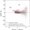 |
Fig. 12 Photometric equivalent width as a function of the (mF555W−mF814W) colour. Grey points are all the objects that passed the photometric selection, while red points are the candidate Hα emitters. The dotted line marks the minimum pEW of the candidate Hα emitters. We plot in blue the candidate optical counterpart that we found to have an Hα excess. |
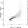 |
Fig. 13 Colour–colour diagram constructed with (mF555W−mF658N) versus (mF555W−mF814W) colours. Grey points are stars passing the photometric selection by Libralato et al. (2018) and membership selection. The blue dots represent our candidate counterparts for which we found an Hα excess with the method described in Sect. 3.3. |
4.3.1 X6c
This star is one of the four objects falling inside the uncertainty radius for the X-ray source X6. Its position in the (mF555W, mF390W−mF555W) CMD resembles that of X5c, as it is located between the MS and the WD cooling sequence, while it shifts towards the WD cooling sequence in the (mF225W, mF225W−. mF275W) CMD, suggesting that this could be a system containing a WD. The proper motion diagram suggests that this object is a cluster member. Figure 8 clearly shows that this star, has a significant (mF555W−mF658N) colour excess. Moreover, its pEW of 46.5 Å is the highest among the X-ray counterparts with Hα emission. As a reference, in the analysis performed by Pallanca et al. (2017) on the Hα emitters of NGC 6397, the objects with the highest Hα excess are 7 CVs, with pEW ranging from a minimum of 15.2 Å to a maximum of 90.4 Å, as reported in their table 1. The pEW of X6c falls precisely within this range; hence, both the CMD position and the prominent Hα pEW suggest that this object may be a CV. On the other side, as anticipated before and shown in Fig. 13, this excess seems to be absent in the CMD constructed with coeval Hα and R images. As previously noted, the Hα excess detected in our analysis could potentially result from significant long-term variability and/or a transient event, such as a flare in the accretion disc.
4.3.2 X8c
X8c is one of the seven counterparts found for its X-ray source. In the CMD it is located along the RGB and according to Libralato et al. (2018) proper motions is a cluster member. The (mF555W−mF658N) colour excess of X8c is not as remarkable as the one of X6c, and its pEW of 1.86 Å is the lowest among the identified Hα emitters. Given the very low value of the pEW and its CMD position, this system might be an AB with a red giant component.
4.3.3 X20c
This is one of the three SSG counterparts we found in this work, together with X15c and X16Ac. Given its peculiar CMD position, this object was already included in our list of high-confidence counterparts. In this case, the presence of an Hα emission together with the peculiar CMD position suggests even more strongly that this could be the real counterpart to the X-ray source X20. Its emission is also confirmed by the survey on 26 GCs performed by Göttgens et al. (2019) with MUSE (see Sect. 5.1). The value of the pEW we found for X20c is 3.35 Å, the second smallest among the Hα emitters. The census of Hα emitters in NGC 6397 performed by Pallanca et al. (2017) revealed that the MSPs companions COM-6397A and COM-6397B, are among the Hα emitters of NGC 6397, with a pEW of 3.2 Å and 4.3 Å, respectively. Both the values of the pEW and the CMD position of COM-6397B are consistent with our X20c candidate counterpart. Moreover, its light curve does not show any variability; hence, it is possible that, if variable, either this object has a longer period than our temporal baseline or the inclination of the system is such that we do not see variability. Given these characteristics, it is possible that this counterpart might represent an example of spider MSP. On the other side, this object is also consistent in being an AB, both in terms its CMD position and moderate Hα excess. At this time, we cannot dismiss either of the two possibilities.
4.3.4 X23c
We previously discussed this object in Sect. 4.1 and Sect. 4.2 due to its peculiar CMD position and distinct light curve, exhibiting clear variability among the three WFC3 filters. Based on the comparison with the V20 source in Rozyczka et al. (2016), we interpret this object as a close eclipsing binary BSS, where the X-ray emission could be explained by coronal activity. Furthermore, this object displays a significant Hα excess with a pEW of 27.5 Å. In this case, the Hα excess might be related to an ongoing mass transfer process. On the other side, it is worth noticing that, the remarkable variability of this source might also affect the single-epoch measurement of the Hα magnitude.
Candidate optical counterparts showing Hα excess.
4.3.5 X13c and X25Bc
These two objects lie on the cluster’s MS, both in the (mF390W−mF555W) and (mF555W−mF814W) CMDs. Both X13c and X25Bc are classified as cluster members according to the proper motion analysis. They are characterised by moderate values for the pEW, being 12.1 and 7.97 Å for X13c and X25Bc, respectively. However, the fact that their CMD position remains unchanged across different filter combinations suggests the absence of a blue component in this system. Furthermore, considering the moderate Hα excess, it is possible that these two objects are ABs. None of the other counterparts of X13c show any peculiarities, apart from the proximity to the X-ray source, either in their CMD position or light curve. Therefore, the presence of Hα emission in the X13c suggests that it could be the most probable counterpart for this X-ray source. On the other hand, X25Bc is not the only candidate counterpart we identified for the X25 X-ray source. In fact, in addition to X25Bc, we identified another potential counterpart, X25Ac, which is more likely to be the correct identification due to its clear UV excess, suggesting a CV nature.
5 Clues from spectroscopy
5.1 Hα analysis by Göttgens et al. (2019)
Göttgens et al. (2019) identified 156 Hα emitters in 27 Galactic GCs by using MUSE. Within this sample, 7 stars belong to NGC 362. Using the coordinates listed in their Table A.2, we matched them with our catalogue to determine whether any of these 7 objects correspond to candidate counterparts in our list. We were able to identify three of them. As anticipated in Sect. 4.3, our X20c corresponds to the first object listed for NGC 362 in table A.2 of Göttgens et al. (2019). In our analysis we found for this object an Hα excess with a pEW of 3.34 Å. Interestingly, Göttgens et al. (2019) found a variable Hα emission for this source. This additional information provides interesting clues about the nature of this object. As anticipated before, X20c is in the SSG region, which is populated by close binaries, such as close, coronally emitting ABs, or more exotic objects such as RB MSPs. The variability of this star did not show any peculiarity; however, the presence of a variable emission in Hα might suggest that this could be an example of an MSP where the emission is likely produced by a combination of material stripped from the companion and a strong intrabinary shock. The fifth object associated with NGC 362 as listed in Göttgens et al. (2019) corresponds to the optical counterpart to X12. As X20c, this counterpart is also characterised by a variable Hα emission. In the CMDs shown in Fig. 9, X12c lies significantly redwards of the RGB. Given its CMD position and the variable Hα emission found by Göttgens et al. (2019), X12 could be interpreted as an AB system, such as an RSS. In our study, we did not find any photometric evidence of Hα emission for it. Finally, the last object with variable emission listed in Göttgens et al. (2019) corresponds to our counterpart X10c. As anticipated in Sect. 4.1, we also found a match between X10c and the V24 variable star in Rozyczka et al. (2016). Here, this system is interpreted as an eclipsing semidetached binary system, formed by two ∼ 0.8 M⊙ stars, where the primary giant is filling its Roche lobe and the secondary star is a blue object, either a BSS or a WD. Moreover, in our analysis, X10c satisfies the requirement for being considered an Hα emitter, but fails the mF814W photometric selection criterion, both in CHI and SHARP. Although it has a pEW of 13.0 Å, X10c's Hα excess is not significant enough to confidently include it among the confirmed emitters as we did instead for X6c. Nonetheless, the Hα emission detected by Göttgens et al. (2019), would suggest that accretion is taking place in this system, probably through Roche-lobe overflow, as suggested by Rozyczka et al. (2016).
5.2 MUSE radial velocities
Multi-epoch RV measurements are particularly useful for understanding the motion of celestial bodies. In particular, the orbital motion of binary system components causes their RVs to vary periodically. Therefore, detecting regular changes in an object’s RV curve is a strong indication that it may belong to a binary system, with its mass ratio, eccentricity, and inclination shaping the radial velocity modulation. Multi-epoch RVs analysis provide a powerful complementary information to magnitude variability to identify and characterise binary systems.
To gain deeper insights into the nature of our high-confidence counterparts, we examined their RVs across multiple observation epochs. The starting point of this analysis is the survey of 27 Galactic GCs (PI: S. Kamann, formerly S. Dreizler) performed with the integral field spectrograph MUSE at the VLT (Kamann et al. 2018). Here we used observations of NGC 362 obtained in Wide Field Mode (WFM) in three main epochs: November 22, 2014; October 8–13, 2015; and November 2, 2017. The RV measurements were produced by combining individual exposures from each pointing within each 1-hour observing block (OB). Typically, a single OB included observations at four distinct pointings, with each pointing observed three times, resulting in four data cubes per OB. For each star we discarded the measurements with reliability R < 0.8 or flagged as outliers. The methods for reliability assessment and outlier detection are described in Sect. 3.2 of Giesers et al. (2019).
We found that eight out of our 28 high-confidence counterparts (see Sect. 6) have multi-epoch RV measurements. These include the brightest counterparts: X8c, X9c, X10c, X12c, X16Bc, X20c, X21Ac, and X23c. As a first step, to determine whether our high-confidence counterparts exhibited any variation in RV, we applied the method recently proposed by Giesers et al. (2019) in their study of binary systems in NGC 3201. To detect RV variations in a given star with m measurements, they compute the χ2 for the set of measurements xj with uncertainties σj. This determines how consistent the measurements are with a constant weighted mean x̄ (null hypothesis) of the data (see eq. 2 in Giesers et al. 2019). We computed the χ2 for each of the eight counterparts and normalised it by dividing by m−1. In Fig. 14, we plot the reduced chi-square χ2n as a function of the weighted mean of the RV measurements for each star (v̄r). The eight high-confidence counterparts are highlighted with orange diamonds, and their names are labelled. The solid vertical blue line indicates the heliocentric RV of NGC 362, while the dashed lines represent the central 1D velocity dispersion σ0, whose values are taken from the catalogue provided by Baumgardt et al. (2020)5. The black rectangle highlights the area of the plot with χ2 < 10, which is shown in more detail in the zoomed-in inset on the right.
Most of the counterparts shown in the figure have an average RV close to the systemic velocity of the cluster, which supports the membership of these eight objects, as already suggested by the study of their proper motions (see Sect. 4.1). Specifically, all objects fall within 3σ0 of the cluster’s velocity, with the only exception of X10c. However, based on proper motions, X10c appears to be a member of the cluster. On the other hand, it should be noted that X10c has the highest χ2n value among all, exceeding 200, which may indicate significant variability. This variability could, in turn, affect the assessment of its membership when considering the resulting average RV. In general, as also mentioned by Giesers et al. (2019), a star with χ2 > 1 typically exhibits RV variations exceeding the associated uncertainties. This condition holds for all the counterparts shown here, except for X8c, which has a χ2n of 0.58.
In addition to analyzing the χ2 value for each high-confidence counterpart with available multi-epoch RV measurements, we also opted to visually inspect the RV curves for these objects, selecting the ones that displayed the clearest indications of significant variability. By combining the χ2n analysis with a visual inspection of the RV curves, we identified clear variability in the RV of four out of the eight counterparts with available measurements. Specifically, this applies to X10c, X12c, X16Bc, and X21Ac, whose RV curves are presented in Fig. 15. For clarity, the x-axis represents the MJD – MJD0, where MJD0 = 2456983.5076, which corresponds to the epoch of the first observation from the November 2014 dataset. The data points in the plots are colour-coded according to the macro-epoch to which they belong. In fact, as mentioned above, the available RV measurements were obtained from observations grouped into three macro-epochs. Within the same epoch, however, the measurements are taken in close succession, with intervals ranging from a minimum of ∼3 minutes for the November 2014 observations, ∼ 10 minutes for the November 2017 observations, up to approximately one day for the October 2015 observations. Consequently, for each counterpart, there are at most three RV measurements available that are separated by a reasonable temporal interval. This limitation prevented us from conducting period studies on RV curves.
Nonetheless, we can confidently state that X10c, X12c, X16Bc, and X21Ac show significant variability in their RV curves, with amplitudes ranging from ∼38 km s−1 in the case of X10c up to 98 km s−1 for X12c, showing that these four objects belong to binary systems.
Finally, it is worth noting that for X16Bc, we also observed consistent variability in its photometric curve (see Sect. 4.2), identifying a period of 13.44 hours. Due to the reasons outlined earlier, we could not determine an estimate of the period from the analysis of RV curves; hence, we could not make a comparison between the results obtained from photometry and spectroscopy. Nevertheless, this additional analysis supports the hypothesis proposed in Sect. 4.2 that this object likely resides in a binary system. Conversely, no signs of photometric modulation were detected for the other three objects exhibiting RV variability. This absence may be attributed to their significantly longer periods compared to the temporal coverage of our HST observations. This is indeed the case for the X10c, for which Rozyczka et al. (2016) found a period of 8.1 days.
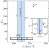 |
Fig. 14 Reduced χ2 as a function of the weighted mean of the RVs for our eight high-confidence counterparts with available multi-epoch RV measurements (orange diamonds). The solid vertical blue line is the heliocentric RV of NGC 362, while the dashed lines represent the central 1D velocity dispersion σ0. The inset on the right is a zoom-in of the area highlighted by the black rectangle. |
6 Conclusions
The photometric search of optical counterparts to X-ray sources in the GC NGC 362 performed in this work yielded 28 high-confidence candidates. Figure 16 shows their location in the (mF225W, mF225W−mF275W), (mF555W, mF390W−mF555W), and (mF555W, mF555W−mF814W) CMDs. We opted to use different colours to denote the distinct criteria leading to the inclusion of counterparts in the final list of the most interesting candidates. Orange points indicate counterparts exhibiting evident variability, while green points denote objects for which we found Hα emission. Additionally, blue points show counterparts occupying peculiar positions in the CMD. X1 is the only case in which we found only one counterpart within the uncertainty radius, and it is highlighted in red. Ten of the high-confidence counterparts we present are in common with those suggested by Kumawat et al. (2024), and they are indicated as squares in Fig. 16. Among the 28 high-confidence counterparts identified in this study, 17 were selected based solely on their peculiar positions in the CMD, five due to their photometric variability, and six for their Hα excess. Notably, four objects satisfy two of these criteria: X5c and X16Bc display both variability and an unusual CMD position, while X20c and X6c combine an anomalous CMD position with Hα excess. Remarkably, X23c fulfills all the criteria established in this analysis. These findings indicate that these five objects are the most intriguing and promising counterparts identified in our work, pointing to their potential association with interacting binary systems, MSPs, or CVs. In Kumawat et al. (2024), only two of these five objects are identified, specifically X16Bc and X20c. This is reasonable, as our identification of the remaining three objects was primarily based on variability and Hα analyses, which were not performed by Kumawat et al. (2024). Additionally, the integration of our photometric analysis with MUSE multi-epoch RV measurements seems to indicate that X10c, X12c, X16Bc, and X21Ac reside in binary systems. A summary of all the high-confidence counterparts proposed in our work is provided in Table A.1.
Kumawat et al. (2024) suggests that the X-ray spectrum of X1 is well fitted by an NS hydrogen atmosphere and interpret this object as a qLMXB. On the other hand, no qLMXB counterpart has ever been found on the SGB of a cluster. To explain this aspect, Kumawat et al. (2024) suggests that either the qLMXB accretion disc is faint and does not appear against a relatively bright star or the real qLMXB companion could be a fainter star. In this regard, as is visible in Fig. A1 of Kumawat et al. (2024), there is a fainter star close to the position of X1 that lacks HUGS photometry. We also could not find this star in the WFC3 images, where we only recovered the same counterpart reported in Kumawat et al. (2024). However, thanks to the HRC database, we were able to obtain the F435W photometry for the fainter star. Its magnitude is ∼1.5 mag fainter with respect to the SGB counterpart; however, we could not assess its position in the CMD since we only have one magnitude available. In addition, it does not show any evidence of variability. Nevertheless, our photometry differs from the HUGS photometry used by Kumawat et al. (2024), which places X1c in the SSG region, whereas our photometry situates it on the SGB. This shift makes the star a less likely candidate counterpart.
We identified the same optical counterparts as Kumawat et al. (2024) for X9 and X10, which lie redward of the RGB in the (mF555W, mF555W−mF814W) CMD but lie substantially blueward of the RGB in the (mF225W, mF225W−mF275W), suggesting very blue and red light sources. Additionally, the match we performed with the stars analysed by Göttgens et al. (2019) revealed that X10c exhibits variable Hα emission, and its RV curve suggests that this object might be in a binary system.
Standing out among the promising counterparts identified by Kumawat et al. (2024) are X15c, X16c, and X20c. All three are classified as SSGs and are located below the MSTO in the CMD. As previously mentioned, we also included these three objects because of their CMD position. Moreover, for X20c, we also found evidence of Hα emission, which has also been spectroscopically confirmed by Göttgens et al. (2019, see Sect. 5.1).
Concerning their counterparts proposed for the X12 and X21A sources, we agree with the hypothesis that given their CMD position, these counterparts appear to be RSSs with X-rays driven by chromospheric activity. Moreover, for both of them, we found RV curves showing strong variability, suggesting that they could be residing in binary systems. Finally, the Hα emission found by Göttgens et al. (2019) for X12c, together with the X-ray emission, corroborates the hypothesis that this system is characterised by intense chromospheric activity.
Among the other candidate ABs found by Kumawat et al. (2024), there are five counterparts they called X21B, X23A, X23B, X23C, and X26. Since these objects do not meet our criteria, we did not include them among our final list of high-confidence counterparts.
Finally, Kumawat et al. (2024) identified X4 and X24 as two background galaxies. We confirmed their identification of the same counterparts for both X4 and X24 sources within their uncertainty radius and included them due to their peculiar CMD position.
Of the remaining 18 high-confidence counterparts, ten are not present in the HUGS catalogue used by Kumawat et al. (2024), namely, X2c, X6c, X7c, X17c, X18Ac, X18Bc, X19c, X21Bc, X25Ac, and X33c. Of the remaining eight candidates, X5c, X16Bc, and X23c are included in our list due to their variability, while X8c, X13c, and X25Bc exhibit Hα emission. Lastly, we included X24Bc and X28c due to their peculiar positions in the CMDs. Finally, it is worth noting that Kumawat et al. (2024) did not find any CV candidate, although they calculated that some CV systems are expected to be present in NGC 362, as suggested by extrapolation of the stellar encounter rate from 47 Tucanae. They attributed this aspect to the optical crowding in the core of the cluster. On the other hand, our identification of several CV candidates (X2c, X5c, X6c, X17c, X19c, X18Ac, X18Bc, X25Ac, and X28c) demonstrates that our photometry is more effective at identifying faint blue stars compared to the HUGS photometry. We attribute this to the fact that the HUGS photometry relies on the F555W and F814W star catalogs for its master list. As shown in our CMDs, many faint blue stars that are clearly visible in bluer filters remain undetectable in F555W and F814W. This is either due to the presence of nearby bright stars in the redder filters or because the stars are too blue and faint to be captured in these redder bands.
In conclusion, the comprehensive methodology used in this study – integrating multi-wavelength, multi-epoch, and multiinstrument data – along with the synergy between optical and X-ray observations has been essential in advancing our understanding of the nature of the studied systems. Moreover, future timing studies of MSPs in NGC 362 will be pivotal to confirming our candidates by linking our variability measures and period estimates to precise orbital periods as derived from radio observations. In addition, the proposed MSP optical counterparts identified in this work will contribute to ongoing radio analyses with MeerKAT, facilitating the identification and comprehensive characterisation of MSPs in NGC 362.
 |
Fig. 15 From left to right, RV curves for the optical counterparts X10c, X12c, X16Bc, and X21Ac obtained from MUSE observations of NGC 362 in November 22, 2014; October 8–13, 2015; and November 2, 2017. The data points in the plots are colour-coded according to the macro-epoch to which they belong. The x-axis represents the MJD – MJD0, where MJD0 = 2456983.5075578704 is the MJD of the first observation from the November 22, 2014 dataset. |
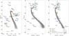 |
Fig. 16 Colour-magnitude diagrams containing the 28 high-confidence optical counterparts found in this study. From left to right, (mF225W, mF225W−mF275W), (mF555W, mF390W−mF555W), and (mF555W, mF555W−mF814W). Orange points indicate counterparts exhibiting evident variability, while green points denote objects for which we found an Hα emission. Additionally, blue counterparts indicate those occupying interesting positions in the CMD. Red counterparts are the only counterparts found within the uncertainty radius of their respective X-ray source. Squares indicate those counterparts that we find in common with Kumawat et al. (2024). |
Acknowledgements
We acknowledge financial support from the INAF Data Analysis Research Grant (ref. E. Dalessandro) of the ‘Bando Astrofisica Fondamentale 2024’. The research activities described in this paper were carried out with contribution of the Next Generation EU funds within the National Recovery and Resilience Plan (PNRR), Mission 4 – Education and Research, Component 2 – From Research to Business (M4C2), Investment Line 3.1 – Strengthening and creation of Research Infrastructures, Project IR0000034 – “STILES – Strengthening the Italian Leadership in ELT and SKA”. This work has been funded using resources from the INAF Large Grant 2022 “GCjewels” (PI Andrea Possenti) approved with the Presidential Decree 30/2022. S.D. acknowledges the support of the Deutsche Forschungsgemeinschaft (DFG) through project DR 281/41-1. S.D. acknowledges the support by the BMBF from the ErUM program through grants 05A14MGA, 05A17MGA, 05A20MGA. C.O.H. is supported by NSERC Discovery Grant RGPIN-2023-04264. The authors thank the anonymous referee for their suggestions and comments, which improved the clarity of this work. G.E. is grateful to A. Della Croce for the useful discussions and comments.
Appendix A Summary table
High-confidence optical counterparts identified in this work.
Appendix B Finding charts
In Fig. B.1 we present the finding charts for our 28 high-confidence counterparts. All images are captured using the F390W filter of the WFC3, except for the finding charts of X2c, X18A − Bc, X28c, and X33c, whose images were taken with the F275W filter of the WFC3. The finding charts for X5c and X17c are shown in the main text of the paper, in Fig. 6 and Fig. 11, respectively.
 |
Fig. B.1 Finding charts of our high-confidence counterparts. Each square covers an area of 2.4′′ on each side. In each panel, the X-ray source position is indicated by a blue cross, along with a blue circle whose radius represents the uncertainty in the X-ray position, uncX. The red circle marks the location of the optical counterpart. All the finding charts are oriented in the same way as indicated by the arrows in the first finding chart for X1c. |
References
- Aguado-Agelet, F., Massari, D., Monelli, M., et al. 2025, arXiv e-prints [arXiv:2502.20436] [Google Scholar]
- Archibald, A. M., Stairs, I. H., Ransom, S. M., et al. 2009, Science, 324, 1411 [Google Scholar]
- Astropy Collaboration (Robitaille, T. P., et al.,) 2013, A&A, 558, A33 [NASA ADS] [CrossRef] [EDP Sciences] [Google Scholar]
- Astropy Collaboration (Price-Whelan, A. M., et al.,) 2018, AJ, 156, 123 [Google Scholar]
- Bacon, R., Accardo, M., Adjali, L., et al. 2010, SPIE Conf. Ser., 7735, 773508 [Google Scholar]
- Bailyn, C. D., 1995, ARA&A, 33, 133 [NASA ADS] [CrossRef] [Google Scholar]
- Baluev, R. V., 2008, MNRAS, 385, 1279 [Google Scholar]
- Bassa, C., Pooley, D., Homer, L., et al. 2004, ApJ, 609, 755 [NASA ADS] [CrossRef] [Google Scholar]
- Bassa, C., Pooley, D., Homer, L., et al. 2005, ApJ, 619, 1189 [Google Scholar]
- Baumgardt, H., Sollima, A., & Hilker, M., 2020, PASA, 37, e046 [Google Scholar]
- Beccari, G., De Marchi, G., Panagia, N., & Pasquini, L., 2014, MNRAS, 437, 2621 [Google Scholar]
- Bellazzini, M., Pasquali, A., Federici, L., Ferraro, F. R., & Pecci, F. F., 1995, ApJ, 439, 687 [Google Scholar]
- Bellini, A., & Bedin, L. R., 2009, PASP, 121, 1419 [CrossRef] [Google Scholar]
- Benvenuto, O. G., De Vito, M. A., & Horvath, J. E., 2014, ApJ, 786, L7 [NASA ADS] [CrossRef] [Google Scholar]
- Benvenuto, O. G., De Vito, M. A., & Horvath, J. E., 2015, ApJ, 798, 44 [Google Scholar]
- Bianchini, P., Webb, J. J., Sills, A., & Vesperini, E., 2018, MNRAS, 475, L96 [CrossRef] [Google Scholar]
- Bogdanov, S., Grindlay, J. E., Heinke, C. O., et al. 2006, ApJ, 646, 1104 [NASA ADS] [CrossRef] [Google Scholar]
- Bogdanov, S., van den Berg, M., Heinke, C. O., et al. 2010, ApJ, 709, 241 [CrossRef] [Google Scholar]
- Bond, H. E., White, R. L., Becker, R. H., & O’Brien, M. S., 2002, PASP, 114, 1359 [NASA ADS] [CrossRef] [Google Scholar]
- Cadelano, M., Pallanca, C., Ferraro, F. R., et al. 2015, ApJ, 807, 91 [Google Scholar]
- Cadelano, M., Ferraro, F. R., Istrate, A. G., et al. 2019, ApJ, 875, 25 [NASA ADS] [CrossRef] [Google Scholar]
- Cadelano, M., Chen, J., Pallanca, C., et al. 2020, ApJ, 905, 63 [NASA ADS] [CrossRef] [Google Scholar]
- Carretta, E., Bragaglia, A., Gratton, R. G., et al. 2013, A&A, 557, A138 [NASA ADS] [CrossRef] [EDP Sciences] [Google Scholar]
- Ceccarelli, E., Mucciarelli, A., Massari, D., Bellazzini, M., & Matsuno, T., 2024, A&A, 691, A226 [NASA ADS] [CrossRef] [EDP Sciences] [Google Scholar]
- Chatterjee, S., Gaensler, B. M., Melatos, A., Brisken, W. F., & Stappers, B. W., 2007, ApJ, 670, 1301 [Google Scholar]
- Chen, H.-L., Chen, X., Tauris, T. M., & Han, Z., 2013, ApJ, 775, 27 [NASA ADS] [CrossRef] [Google Scholar]
- Clark, G. W., 1975, ApJ, 199, L143 [NASA ADS] [CrossRef] [Google Scholar]
- Cocozza, G., Ferraro, F. R., Possenti, A., et al. 2008, ApJ, 679, L105 [Google Scholar]
- Cohn, H. N., Lugger, P. M., Couch, S. M., et al. 2010, ApJ, 722, 20 [Google Scholar]
- Cool, A. M., Grindlay, J. E., Cohn, H. N., Lugger, P. M., & Slavin, S. D., 1995, ApJ, 439, 695 [NASA ADS] [CrossRef] [Google Scholar]
- Dalessandro, E., Lanzoni, B., Ferraro, F. R., et al. 2008a, ApJ, 677, 1069 [NASA ADS] [CrossRef] [Google Scholar]
- Dalessandro, E., Lanzoni, B., Ferraro, F. R., et al. 2008b, ApJ, 681, 311 [NASA ADS] [CrossRef] [Google Scholar]
- Dalessandro, E., Ferraro, F. R., Massari, D., et al. 2013, ApJ, 778, 135 [NASA ADS] [CrossRef] [Google Scholar]
- De Marchi, G., Panagia, N., & Romaniello, M., 2010, ApJ, 715, 1 [NASA ADS] [CrossRef] [Google Scholar]
- de Martino, D., Papitto, A., Belloni, T., et al. 2015, MNRAS, 454, 2190 [NASA ADS] [CrossRef] [Google Scholar]
- Dempsey, R. C., Linsky, J. L., Fleming, T. A., & Schmitt, J. H. M. M., 1997, ApJ, 478, 358 [NASA ADS] [CrossRef] [Google Scholar]
- De Vito, M. A., Benvenuto, O. G., & Horvath, J. E., 2020, MNRAS, 493, 2171 [Google Scholar]
- Dickson, N., Smith, P. J., Hénault-Brunet, V., Gieles, M., & Baumgardt, H., 2024, MNRAS, 529, 331 [NASA ADS] [CrossRef] [Google Scholar]
- Dotter, A., Sarajedini, A., Anderson, J., et al. 2010, ApJ, 708, 698 [Google Scholar]
- Edmonds, P. D., Gilliland, R. L., Camilo, F., Heinke, C. O., & Grindlay, J. E., 2002, ApJ, 579, 741 [NASA ADS] [CrossRef] [Google Scholar]
- Edmonds, P. D., Gilliland, R. L., Heinke, C. O., & Grindlay, J. E., 2003, ApJ, 596, 1177 [NASA ADS] [CrossRef] [Google Scholar]
- Ferraro, F. R., Possenti, A., D’Amico, N., & Sabbi, E., 2001, ApJ, 561, L93 [NASA ADS] [CrossRef] [Google Scholar]
- Ferraro, F. R., Beccari, G., Dalessandro, E., et al. 2009, Nature, 462, 1028 [NASA ADS] [CrossRef] [Google Scholar]
- Ferraro, F. R., Lanzoni, B., Dalessandro, E., et al. 2012, Nature, 492, 393 [Google Scholar]
- Ferraro, F. R., Pallanca, C., Lanzoni, B., et al. 2015, ApJ, 807, L1 [NASA ADS] [CrossRef] [Google Scholar]
- Freire, P. C. C., Ransom, S. M., Bégin, S., et al. 2008, ApJ, 675, 670 [NASA ADS] [CrossRef] [Google Scholar]
- Gaia Collaboration (Vallenari, A., et al.,) 2023, A&A, 674, A1 [NASA ADS] [CrossRef] [EDP Sciences] [Google Scholar]
- Geller, A. M., Leiner, E. M., Bellini, A., et al. 2017, ApJ, 840, 66 [NASA ADS] [CrossRef] [Google Scholar]
- Giesers, B., Kamann, S., Dreizler, S., et al. 2019, A&A, 632, A3 [NASA ADS] [CrossRef] [EDP Sciences] [Google Scholar]
- Göttgens, F., Husser, T.-O., et al., Kamann, S., 2019, A&A, 631, A118 [NASA ADS] [CrossRef] [EDP Sciences] [Google Scholar]
- Güdel, M., 2004, A&A Rev., 12, 71 [Google Scholar]
- Harris, W. E., 1996, AJ, 112, 1487 [Google Scholar]
- Heinke, C. O., Grindlay, J. E., Lugger, P. M., et al. 2003, ApJ, 598, 501 [NASA ADS] [CrossRef] [Google Scholar]
- Heinke, C. O., Grindlay, J. E., Edmonds, P. D., et al. 2005, ApJ, 625, 796 [NASA ADS] [CrossRef] [Google Scholar]
- Hertz, P., & Grindlay, J. E., 1983, ApJ, 267, L83 [NASA ADS] [CrossRef] [Google Scholar]
- Hui, C. Y., Cheng, K. S., & Taam, R. E., 2010, ApJ, 714, 1149 [Google Scholar]
- Ivanova, N., Heinke, C. O., Rasio, F. A., et al. 2006, MNRAS, 372, 1043 [CrossRef] [Google Scholar]
- Kamann, S., Husser, T. O., Dreizler, S., et al. 2018, MNRAS, 473, 5591 [NASA ADS] [CrossRef] [Google Scholar]
- Kızıltan, B., Baumgardt, H., & Loeb, A., 2017, Nature, 542, 203 [Google Scholar]
- Knigge, C., 2012, Mem. Soc. Astron. Italiana, 83, 549 [NASA ADS] [Google Scholar]
- Knigge, C., Zurek, D. R., Shara, M. M., Long, K. S., & Gilliland, R. L., 2003, ApJ, 599, 1320 [Google Scholar]
- Kumawat, G., Heinke, C. O., Cohn, H. N., & Lugger, P. M., 2024, MNRAS, 530, 82 [Google Scholar]
- Lanzoni, B., Ferraro, F. R., Alessandrini, E., et al. 2016, ApJ, 833, L29 [NASA ADS] [CrossRef] [Google Scholar]
- Leiner, E., Mathieu, R. D., & Geller, A. M., 2017, ApJ, 840, 67 [NASA ADS] [CrossRef] [Google Scholar]
- Libralato, M., Bellini, A., van der Marel, R. P., et al. 2018, ApJ, 861, 99 [CrossRef] [Google Scholar]
- Libralato, M., Bellini, A., Vesperini, E., et al. 2022, ApJ, 934, 150 [NASA ADS] [CrossRef] [Google Scholar]
- Lomb, N. R., 1976, Ap&SS, 39, 447 [Google Scholar]
- Meurer, G. R., Lindler, D. J., Blakeslee, J., et al. 2003, SPIE Conf. Ser., 4854, 507 [Google Scholar]
- Modiano, D., Parikh, A. S., & Wijnands, R., 2020, A&A, 634, A132 [NASA ADS] [CrossRef] [EDP Sciences] [Google Scholar]
- Moffat, A. F. J., 1969, A&A, 3, 455 [NASA ADS] [Google Scholar]
- Nardiello, D., Libralato, M., Piotto, G., et al. 2018, MNRAS, 481, 3382 [NASA ADS] [CrossRef] [Google Scholar]
- Negoro, H., Kohama, M., Serino, M., et al. 2016, PASJ, 68, S1 [Google Scholar]
- Pallanca, C., Dalessandro, E., Ferraro, F. R., et al. 2010, ApJ, 725, 1165 [CrossRef] [Google Scholar]
- Pallanca, C., Dalessandro, E., Ferraro, F. R., Lanzoni, B., & Beccari, G., 2013, ApJ, 773, 122 [NASA ADS] [CrossRef] [Google Scholar]
- Pallanca, C., Ransom, S. M., Ferraro, F. R., et al. 2014, ApJ, 795, 29 [NASA ADS] [CrossRef] [Google Scholar]
- Pallanca, C., Beccari, G., Ferraro, F. R., et al. 2017, ApJ, 845, 4 [NASA ADS] [CrossRef] [Google Scholar]
- Papitto, A., Bozzo, E., Ferrigno, C., & Rea, N., 2013, ATel, 5534, 1 [Google Scholar]
- Paresce, F., de Marchi, G., & Ferraro, F. R., 1992, Nature, 360, 46 [NASA ADS] [CrossRef] [Google Scholar]
- Penny, A. J., 1976, PhD thesis, Sussex University, UK [Google Scholar]
- Pietrukowicz, P., Kaluzny, J., Schwarzenberg-Czerny, A., et al. 2008, MNRAS, 388, 1111 [Google Scholar]
- Piotto, G., Milone, A. P., Bedin, L. R., et al. 2015, AJ, 149, 91 [Google Scholar]
- Pooley, D., & Hut, P., 2006, ApJ, 646, L143 [NASA ADS] [CrossRef] [Google Scholar]
- Pooley, D., Lewin, W. H. G., Homer, L., et al. 2002, ApJ, 569, 405 [Google Scholar]
- Reynolds, M. T., Callanan, P. J., Fruchter, A. S., et al. 2007, MNRAS, 379, 1117 [NASA ADS] [CrossRef] [Google Scholar]
- Roberts, M. S. E., 2013, in Neutron Stars and Pulsars: Challenges and Opportunities after 80 years, 291, ed. J. van Leeuwen, 127 [NASA ADS] [Google Scholar]
- Rozyczka, M., Thompson, I. B., Narloch, W., Pych, W., & SchwarzenbergCzerny, A., 2016, Acta Astron., 66, 307 [Google Scholar]
- Rucinski, S. M., 2000, AJ, 120, 319 [Google Scholar]
- Saito, Y., Kawai, N., Kamae, T., et al. 1997, ApJ, 477, L37 [Google Scholar]
- Scargle, J. D., 1982, ApJ, 263, 835 [Google Scholar]
- Shara, M. M., Hinkley, S., Zurek, D. R., Knigge, C., & Dieball, A., 2005, AJ, 130, 1829 [Google Scholar]
- Sirianni, M., Jee, M. J., Benítez, N., et al. 2005, PASP, 117, 1049 [Google Scholar]
- Smedley, S. L., Tout, C. A., Ferrario, L., & Wickramasinghe, D. T., 2015, MNRAS, 446, 2540 [Google Scholar]
- Stetson, P. B., 1987, PASP, 99, 191 [Google Scholar]
- Stetson, P. B., 1994, PASP, 106, 250 [Google Scholar]
- Stetson, P. B., 1996, PASP, 108, 851 [NASA ADS] [CrossRef] [Google Scholar]
- Tauris, T. M., & Savonije, G. J., 1999, A&A, 350, 928 [NASA ADS] [Google Scholar]
- Turk, P. J., & Lorimer, D. R., 2013, MNRAS, 436, 3720 [Google Scholar]
- van Dokkum, P. G., 2001, PASP, 113, 1420 [Google Scholar]
- Verbunt, F., Kuiper, L., Belloni, T., et al. 1996, A&A, 311, L9 [NASA ADS] [Google Scholar]
- Verbunt, F., Pooley, D., & Bassa, C., 2008, in Dynamical Evolution of Dense Stellar Systems, 246, eds. E. Vesperini M. Giersz & A. Sills 301 [Google Scholar]
- Wadiasingh, Z., Harding, A. K., Venter, C., Böttcher, M., & Baring, M. G., 2017, ApJ, 839, 80 [NASA ADS] [CrossRef] [Google Scholar]
- Witham, A. R., Knigge, C., Gänsicke, B. T., et al. 2006, MNRAS, 369, 581 [NASA ADS] [CrossRef] [Google Scholar]
- Zavlin, V. E., Pavlov, G. G., Sanwal, D., et al. 2002, ApJ, 569, 894 [Google Scholar]
- Zhang, L., Ridolfi, A., Blumer, H., et al. 2022, ApJ, 934, L21 [Google Scholar]
- Zhang, L., Freire, P. C. C., Ridolfi, A., et al. 2023, ApJS, 269, 56 [NASA ADS] [CrossRef] [Google Scholar]
- Zhao, J., & Heinke, C. O., 2022, MNRAS, 511, 5964 [NASA ADS] [CrossRef] [Google Scholar]
Our dataset spans a quite limited temporal baseline, allowing us to detect variability only in objects with relatively short periods.
The catalogue is publicly available at https://people.smp.uq.edu.au/HolgerBaumgardt/globular/. Values used in this work are from the 4th version of the catalogue updated in March 2023.
This corresponds to the candidate counterpart identified as X16 in Kumawat et al. (2024)
This is not the same counterpart as the X21B identified by Kumawat et al. (2024)
Our candidate counterpart for the X23 X-ray source does not match any of the three candidates, X23A, X23B, and X23C, suggested by Kumawat et al. (2024) for the same source. Indeed their X23A, X23B, and X23C do not fulfill any of the criteria established in this paper for identifying high-confidence counterparts. On the other side, our X23c shows both significant photometric variability and Hα excess, in addition to its peculiar CMD position.
All Tables
All Figures
|
Fig. 1 Footprints of the FoVs covered by the HST observations listed in Table 1. The underlying stars come from the Gaia DR3 dataset (Gaia Collaboration 2023) centred on NGC 362, obtained with a search radius of 1 degree and using the Gaia G-band magnitude to scale the size of the data points. Each FoV is colour-coded according to the GO proposal number, listed in Table 1. The black cross marks the centre (RA = 15.8087453, Dec = −70.8489012, Dalessandro et al. 2013) while the black circle represents the half-mass radius, rh (63′′.5, Dalessandro et al. 2013). |
| In the text | |
|
Fig. 2 Zoomed-in version of Fig. 1. Red circles represent the 33 X-ray sources identified by Kumawat et al. (2024). Each source is labelled with a number, following the nomenclature established by Kumawat et al. (2024). The black circle marks the core radius, rc (13′′.0, Dalessandro et al. 2013). |
| In the text | |
|
Fig. 3 Left: full proper motion VPD from the HSTPROMO catalogue. Right: proper motion VPD for stars within the F606W magnitude bin that includes one of the candidate counterparts of X5 (the object shown in blue in Fig. 6). The purple point indicates the object’s position in the VPD along with its associated errors. The blue, orange and red circles represent the 1σ, 2σ, and 3σ contours, respectively. |
| In the text | |
|
Fig. 4 CHI parameter (top panel) and SHARP parameter (bottom panel) as a function of mF814W magnitude. Objects in red represent selected stars following the 3σ-rejection method, while black points are rejected stars. The solid black line represents the average CHI (top panel) and average SHARP (lower panel). It can be observed that both CHI and SHARP display an irregular pattern at brighter magnitudes, particularly for mF814W < 17. This irregularity occurs due to the saturation affecting the magnitudes of these stars. Consequently, the average and standard deviation within these bins are affected, leading to the observed behaviour. |
| In the text | |
|
Fig. 5 Data selection process schematically illustrated in (mF555W, mF390W−mF555W) CMDs. The left panel shows the observed CMD, including all detected stars. The middle panel shows the cleaned CMD after photometric quality cuts. The fraction of stars removed according to photometric quality cuts is 0.53. It can be observed that the stars in the upper part of the RGB and those on the horizontal branch are excluded after the photometric quality cuts, which is a result of saturation. The right panel shows the final CMD after membership selection. The fraction of stars removed according to membership evaluation with respect to the complete catalogue shown in the first panel is 0.05. |
| In the text | |
|
Fig. 6 Finding chart for source X5 in the F390W WFC3 band covering an area of 2.4′′ on each side. The cyan circle is centred on the X-ray position, indicated by a cyan cross, and it has a radius equal to the X-ray position uncertainty uncX. The magenta circles denote the positions of the candidate counterparts. We mark in blue the candidate counterpart X5c, which is the same as the one presented in Figs. 3 and 7. |
| In the text | |
|
Fig. 7 Global light curve of one candidate counterpart to the X5 source (object marked in blue in Fig. 6) obtained by combining the data points from F390W, F555W, and F814W WFC3 images (in green, orange and red respectively). The light curve is folded with a period of 5.08 hours, obtained from the Lomb-Scargle analysis. The grey solid line, a combination of sines and cosines fitted to the data points. It has no physical meaning, it is plotted only to facilitate the visualisation of the curve. |
| In the text | |
|
Fig. 8 Colour-colour diagram constructed with (mF555W−mF658N) versus (mF555W−mF814W) colours. Grey points are stars passing the photometric and membership selection. Candidate Hα emitters are represented in red. We plot in blue the candidate optical counterparts that we found to have an Hα excess (see Sect. 4.3). |
| In the text | |
|
Fig. 9 From left to right, CMDs of (mF225W, mF225W−mF275W), (mF555W, mF390W−mF555W), and (mF555W, mF555W−mF814W). Counterparts showing peculiar CMD position are plotted in blue. Objects that become bluer in the mF390W−mF555W CMD might have an accretion disc and/or a WD. Squares indicate those counterparts that were identified also by Kumawat et al. (2024). The step observed along the RGB at mF555W ∼ 17 in the (mF555W, mF555W−mF814W) CMD is due to issues related to saturation in the F814W filter. |
| In the text | |
|
Fig. 10 From left to right, top to bottom: Global light curves of X7c, X16Bc, X23c, and X33c. The light curve of X7c does not show mF225w and mF275W measurements for clarity. The curves are folded using periods of 8.89 hours, 13.44 hours, 9.53 hours and 3.10 hours respectively, determined from Lomb-Scargle analysis performed on the global curves across all available filters. In each panel, the grey solid line is a combination of sines and cosines fitted to the data points with the only purpose of helping the visualisation of the light curve. |
| In the text | |
|
Fig. 11 Four HST combined and calibrated images (.drz file for the F435W filter and .drc files for the other three filters) centred on the position of the X-ray source X17. In the top-left panel, the F435W image from the December 2004 ACS/HRC observation is shown. The image in the top-right panel was taken in the F390W filter as part of the WFC3/UVIS observations of April 2012. The bottom panels, from left to right, display the F225W and F275W WFC3/UVIS images from September 2016. In each panel, the X-ray source position is indicated by a cyan cross, along with a cyan circle whose radius represents the uncertainty in the X-ray position, uncX. The red circle marks the location of the counterpart X17c. |
| In the text | |
|
Fig. 12 Photometric equivalent width as a function of the (mF555W−mF814W) colour. Grey points are all the objects that passed the photometric selection, while red points are the candidate Hα emitters. The dotted line marks the minimum pEW of the candidate Hα emitters. We plot in blue the candidate optical counterpart that we found to have an Hα excess. |
| In the text | |
|
Fig. 13 Colour–colour diagram constructed with (mF555W−mF658N) versus (mF555W−mF814W) colours. Grey points are stars passing the photometric selection by Libralato et al. (2018) and membership selection. The blue dots represent our candidate counterparts for which we found an Hα excess with the method described in Sect. 3.3. |
| In the text | |
|
Fig. 14 Reduced χ2 as a function of the weighted mean of the RVs for our eight high-confidence counterparts with available multi-epoch RV measurements (orange diamonds). The solid vertical blue line is the heliocentric RV of NGC 362, while the dashed lines represent the central 1D velocity dispersion σ0. The inset on the right is a zoom-in of the area highlighted by the black rectangle. |
| In the text | |
|
Fig. 15 From left to right, RV curves for the optical counterparts X10c, X12c, X16Bc, and X21Ac obtained from MUSE observations of NGC 362 in November 22, 2014; October 8–13, 2015; and November 2, 2017. The data points in the plots are colour-coded according to the macro-epoch to which they belong. The x-axis represents the MJD – MJD0, where MJD0 = 2456983.5075578704 is the MJD of the first observation from the November 22, 2014 dataset. |
| In the text | |
|
Fig. 16 Colour-magnitude diagrams containing the 28 high-confidence optical counterparts found in this study. From left to right, (mF225W, mF225W−mF275W), (mF555W, mF390W−mF555W), and (mF555W, mF555W−mF814W). Orange points indicate counterparts exhibiting evident variability, while green points denote objects for which we found an Hα emission. Additionally, blue counterparts indicate those occupying interesting positions in the CMD. Red counterparts are the only counterparts found within the uncertainty radius of their respective X-ray source. Squares indicate those counterparts that we find in common with Kumawat et al. (2024). |
| In the text | |
|
Fig. B.1 Finding charts of our high-confidence counterparts. Each square covers an area of 2.4′′ on each side. In each panel, the X-ray source position is indicated by a blue cross, along with a blue circle whose radius represents the uncertainty in the X-ray position, uncX. The red circle marks the location of the optical counterpart. All the finding charts are oriented in the same way as indicated by the arrows in the first finding chart for X1c. |
| In the text | |
Current usage metrics show cumulative count of Article Views (full-text article views including HTML views, PDF and ePub downloads, according to the available data) and Abstracts Views on Vision4Press platform.
Data correspond to usage on the plateform after 2015. The current usage metrics is available 48-96 hours after online publication and is updated daily on week days.
Initial download of the metrics may take a while.