| Issue |
A&A
Volume 688, August 2024
|
|
|---|---|---|
| Article Number | A180 | |
| Number of page(s) | 14 | |
| Section | Stellar structure and evolution | |
| DOI | https://doi.org/10.1051/0004-6361/202450344 | |
| Published online | 23 August 2024 | |
The HST Large Programme on ω Centauri
VI. The radial gradient of the stellar populations⋆
1
Dipartimento di Fisica e Scienze della Terra, Università di Ferrara, Via Giuseppe Saragat 1, Ferrara 44122, Italy
2
Istituto Nazionale di Astrofisica, Osservatorio Astronomico di Padova, Vicolo dell’Osservatorio 5, Padova 35122, Italy
e-mail: michele.scalco@inaf.it
3
Department of Astronomy, Indiana University, Swain West, 727 E. 3rd Street, Bloomington, IN 47405, USA
Received:
12
April
2024
Accepted:
29
May
2024
In this paper we present the analysis of Hubble Space Telescope (HST) observations of the globular cluster Omega Centauri. Our analysis combines data obtained in this work with previously published HST data from an earlier article of this series and encompasses a broad portion of the cluster’s radial extension. Our findings reveal a significant radial variation in the fraction of stars within the two largest stellar populations, showing that one of the main second-population groups (referred to as the blue main sequence (bMS) group) is more centrally concentrated than the first-population group (referred to as the red main sequence (rMS) group). Additionally, we explore the spatial variations of the other, smaller stellar populations (referred to as MSa and MSd) and find a qualitatively similar, but weaker, radial decrease in the fraction of stars in these populations at larger distances from the cluster centre. Only one of the populations identified (MSe) does not show any significant radial variation.
Key words: techniques: photometric / Hertzsprung-Russell and C-M diagrams / globular clusters: individual: NGC5139
The supplementary data are available at the CDS via anonymous ftp to cdsarc.cds.unistra.fr (130.79.128.5) or via https://cdsarc.cds.unistra.fr/viz-bin/cat/J/A+A/688/A180
© The Authors 2024
 Open Access article, published by EDP Sciences, under the terms of the Creative Commons Attribution License (https://creativecommons.org/licenses/by/4.0), which permits unrestricted use, distribution, and reproduction in any medium, provided the original work is properly cited.
This article is published in open access under the Subscribe to Open model. Subscribe to A&A to support open access publication.
1. Introduction
Photometric and spectroscopic studies over the last 20 years have revealed that stars within globular clusters (GCs) exhibit distinct chemical compositions, and can be categorised into two main populations, each potentially containing subpopulations. The stars of the first population (1P) closely resemble the stars of the halo field in terms of chemical composition, whereas the stars of the second population (2P) display depletions in certain light elements, such as carbon, oxygen, and magnesium, along with enrichment in elements such as helium, nitrogen, aluminium, and sodium compared to 1P stars (see e.g. the reviews by Smith 1987; Gratton et al. 2019).
Several scenarios have been proposed to explain the formation of multiple stellar populations (mPOPs) in GCs; however, all of them face significant challenges (see Renzini et al. 2015; Bastian & Lardo 2018). The spatial distributions of the different populations provide crucial information necessary to construct a comprehensive understanding of the formation and evolutionary history of GCs, as well as to constrain possible paths for theoretical investigations. According to various formation scenarios (see e.g. D’Ercole et al. 2008; Bekki 2010; Calura et al. 2019), 2P stars are expected to form in more central concentrations in the inner regions of a GC and gradually mix with 1P stars during the cluster’s evolution driven by two-body relaxation.
Omega Centauri (or NGC 5139, hereafter ω Cen), the most massive GC in the Milky Way, presents an intriguing case of mPOPs (Bedin et al. 2004). Characterised by low reddening (E(B − V)∼0.12; Harris 1996, 2010) and located relatively close to the Sun (∼5 kpc), ω Cen is an ideal target for various photometric and spectroscopic investigations. It hosts a complex system of mPOPs, rendering it one of the most enigmatic stellar systems within the Galaxy. It is populated by at least two primary groups of stars, namely the blue main sequence (bMS) group and the red main sequence (rMS) group (see Bedin et al. 2004; Bellini et al. 2009), which exhibit significant differences in their helium content (Y ∼ 0.40 for the helium-rich component; see Norris 2004; King et al. 2012). In a more recent paper, Bellini et al. (2017c) showed that in the core of ω Cen, both bMS and rMS stars are split into three subcomponents, and identified at least 15 subpopulations. The story of the origin of the intricate properties of the stellar populations in ω Cen remains unclear. Several scenarios have been proposed, with different explanations. For example, ω Cen could be the nucleus of a dwarf galaxy absorbed by the Milky Way, or the outcome of the merger of two or more clusters (Norris et al. 1997; Jurcsik 1998; Bekki & Freeman 2003; Pancino et al. 2000; Bekki & Norris 2006; Ibata et al. 2019; van de Ven et al. 2006). ω Cen represents an exceptional laboratory for unravelling many fundamental aspects of the origin of mPOPs. Its long relaxation time (1.1 Gyr in the core and 10 Gyr at the half-mass radius; Harris 1996, 2010) suggests that its present-day spatial and kinematic properties may retain some ‘memory’ of the same properties emerging at the end of the formation and early evolutionary phases. Studies of ω Cen have shown that the bMS is more centrally concentrated than the rMS, residing within ∼2 rc (where rc = 2.37 arcmin is the core radius of the cluster; from Harris 1996, 2010), and that the fraction of bMS stars is similar to that of rMS stars but as the distance from the cluster centre increases, the relative abundance of bMS stars compared to rMS stars declines significantly. Beyond ∼8 arcmin, the relative proportions of bMS and rMS stars remain constant (Sollima et al. 2007; Bellini et al. 2009), although recent investigations suggest an increase in the bMS/rMS ratio at radii larger than ∼20 arcmin (Calamida et al. 2020).
The Hubble Space Telescope (HST) GO-16247 programme (P.I.; Scalco) is designed to expand upon the work conducted by Sollima et al. (2007) and Bellini et al. (2009), who focused solely on the bMS and rMS groups, to include all 15 subpopulations identified in the core of the cluster by Bellini et al. (2017c). This program seeks to investigate, for the first time, the complete radial distribution of all identified mPOPs across the entire extension of the GC ω Cen.
Schematically, the existing HST radial coverage of the cluster, with filter coverage sufficient to effectively separate and identify the mPOPs, can be divided into three parts. Figure 1 shows the locations of the three parts superimposed on an image from the Digital Sky Survey (DSS)1. Part (i) of the radial coverage maps the cluster from the centre out to ∼1 rc and is represented in yellow in Fig. 1. The entire photometric catalogue for this field has been published and analysed by Bellini et al. (2017a,b,c).
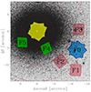 |
Fig. 1. Outlines of the fields observed in HST programs GO-14118+14662 (P.I.: Bedin) and GO-16427 (P.I.: Scalco), superimposed on a DSS image of ω Cen. The primary GO-14118+14662 field (F0) is shown in blue, while the three GO-14118+14662 parallel WFC3 fields are shown in pink. The two GO-16427 fields are shown in green. The data discussed in this paper come from fields F2, F3, F4, and F5. We also show the central field from Bellini et al. (2017a,b,c) in yellow. Units are in arcminutes measured from the cluster centre. The white dashed circle marks the rc while the red dashed circles mark the half-light radius (rh = 5.00 arcmin; from Harris 1996, 2010), and 2 rh and 3 rh from the centre. |
Part (ii) of the radial coverage maps the outskirts of the cluster and consists of three HST fields, mapping between ∼10 arcmin and ∼20 arcmin from the centre of ω Cen, and collected under the multi-cycle programme GO-14118+14662 (P.I.: Bedin). Those fields are represented in pink in Fig. 1 (fields F1, F2, and F3), where we also show the primary field of the GO-14118+14662 programme (field F0) in blue.
The exposures from the parallel fields F1, F2, and F3 were reduced and presented in the five previous publications of this series: the mPOPs at very faint magnitudes in field F1 were analysed by Milone et al. (2017, hereafter Paper I). Bellini et al. (2018, hereafter Paper II) analysed the internal kinematics of the mPOPs in field F1, complementing the GO-14118+14662 data with archival images collected more than 10 years earlier under HST programmes GO-9444 and GO-10101 (King is the P.I. on both). The astrometric catalogue for the F1 field together with the photometry of some filters (F606W, F814W, F110W, and F160W) were released in Paper II. Libralato et al. (2018, hereafter Paper III) presented the absolute proper motion (PM) estimate for ω Cen in the F1 field. Scalco et al. (2021, hereafter Paper IV) released the astro-photometric catalogue for the fields F2 and F3. Finally, Gerasimov et al. (2022, hereafter Paper V) presented a set of stellar models designed to investigate low-mass stars and brown dwarfs in ω Cen.
Part (iii) maps the radial distance between ∼3 arcmin and ∼10 arcmin from the cluster centre. Those fields are represented in green in Fig. 1 (fields F4 and F5) and were observed under programmes GO-12580 (P.I.: Renzini) and GO-14759 (P.I.: Brown) and, more recently, under the GO-16247 programme (P.I.: Scalco). This part of the cluster covers a crucial radial range, because this is where Bellini et al. (2009) found the strongest gradient in the ratio between bMS and rMS stars.
In this paper, we present the reduction of the two intermediate fields F4 and F5 observed under the GO-16247 programme (P.I.: Scalco) and the outer field F1 observed under the GO-14118+14662 programme (P.I.: Bedin), for which the photometry of some filters has not yet been released. Together with the analysis, we also release the catalogue and atlases of the analysed fields. We then combine the photometry obtained from fields F4, F5, and F1 with that from fields F2 and F3 (see Paper IV) and examine the presence of the 15 stellar populations identified by Bellini et al. (2017c) within these fields.
The paper is organised as follows: Section 2 presents the data set and data reduction for fields F4, F5, and F1. Section 3 describes the quality selection and differential-reddening correction applied to the analysed fields F1, F2, F3, F4, and F5, while Section 4 outlines the process used to identify and separate the mPOPs in these fields. Section 5 discusses the radial variations observed among the identified populations. Finally, Section 6 presents a brief summary of the results.
2. Data set and reduction
Fields F4 and F5 were observed in 2012, 2016, 2017, and 2022 using the ultraviolet and visible (UVIS) channel of the Wide Field Camera 3 (WFC3). In each field, data were collected with five filters (F275W, F336W, F438W, F606W and F814W). Table 1 reports the complete list of HST observations of fields F4 and F5.
List of HST observations of fields F4 and F5.
Field F1 was observed under the GO-14118+14662 programme in 2015 and 2017 using the F275W, F336W, F438W, F606W, and F814W filters of the WFC3/UVIS channel and the F110W and F160W filters of the WFC3 near-infrared (NIR) channel. While the astrometry and photometry of some filters were published in Paper II, the catalogue contains only data for which reliable PM measurements were possible. To recover the photometry and astrometry for all other stars, we reprocessed the entire F1 dataset from the GO-14118+14662 programme. We refer to Paper II (see Table 1) for a complete description of the field F1 GO-14118+14662 data set.
The data were reduced following the procedure outlined in Paper IV. In summary, this procedure involves two main steps: the ‘first-pass’ and ‘second-pass’ photometry. During the first-pass photometry, we perturbed a set of ‘library’ WFC3/UVIS and WFC3/NIR effective point spread functions (ePSFs, see Anderson & King 2000, 2006) to determine the optimal spatially variable PSF for each image. Then, using these PSFs, we extracted the positions and fluxes of the stars within each image. This extraction was carried out using the FORTRAN code hst1pass (see Anderson 2022). To account for geometric distortion, the stellar positions in each individual exposure catalogue were corrected using the publicly available WFC3/UVIS and WFC3/NIR correction (Bellini et al. 2011; Anderson 2016). For each filter, the positions and magnitudes were transformed to a common reference frame using six-parameter linear transformations and photometric zero points.
We performed the second-pass photometry using the FORTRAN software package KS2, which is based on the software kitchen_sync presented in Anderson et al. (2008). This software routine makes use of the results obtained from the first-pass stage to simultaneously identify and measure stars across all individual exposures and filters. By relying on multiple exposures, KS2 effectively detects and measures faint stars that would otherwise be lost in the noise of individual exposures. The star-finding process is executed through a series of passes, gradually moving from the brightest to the faintest stars. In each iteration, the routine identifies stars that are fainter than those found in the previous iteration, subsequently measuring and subtracting them. This iterative approach ensures that progressively fainter stars are detected and accounted for, enhancing the overall accuracy of the photometric measurements. KS2 employs three distinct methods for measuring stars, with each approach specifically tailored for different magnitude ranges. We refer to Bellini et al. (2017a), Nardiello et al. (2018) and Paper IV for a detailed description of the methods and procedures. To make the catalogue as similar as possible to that of the F1, F2, and F3 fields released by Paper II and Scalco et al. (2021), we performed the star-finding using the F606W and F814W filters. Our final photometric catalogue contains a total of 40 397, 30 929, and 4 015 sources measured in all five filters for the fields F4, F5, and F1, respectively.
The photometry has been zero-pointed into the Vega magnitude system by following the recipe of Bedin et al. (2005) and adopting the photometric zero-points provided by the STScI web page for WFC3/UVIS and WFC3/NIR2. We cross-referenced the stars in our catalogue with the stars in the Gaia Data Release 3 (Gaia DR3, Gaia Collaboration 2016, 2023). The sources found in common were used to anchor our positions (X, Y) to the Gaia DR3 absolute astrometric system.
PMs were computed using the technique described in Paper IV (see also Bellini et al. 2014; Paper II; Paper III; Libralato et al. 2022). This iterative procedure treats each image as an independent epoch and can be summarised in two main steps: first, it transforms the stellar positions from each exposure into a common reference frame through a six-parameter linear transformation. Then, it fits these transformed positions as a function of the epoch using a least-square straight line. The slope of this line, determined after multiple outlier-rejection stages, provides a direct measurement of the PM. High-frequency-variation systematic effects were corrected as described in Paper II; that is, according to the median value of the closest 100 likely cluster members (excluding the target star itself). Finally, we computed the membership probability (MP) of each star by following a method based on PMs described by Balaguer-Núnez et al. (1998) (see also Bellini et al. 2009; Nardiello et al. 2018; Paper IV).
As part of this publication, we are releasing publicly accessible astro-photometric catalogues and atlases derived from this study for fields F4, F5, and F1. These resources are provided in a format identical to the catalogues and atlases made available by Paper IV for fields F2 and F3. For a comprehensive description of these resources, we refer to Paper IV. When available, we also include the corresponding Gaia DR3 identification numbers for sources in our catalogue. For field F1, we also provide the identification number of the corresponding source in the catalogue published in Paper II when the source is available. The supplementary electronic material for this journal will also be accessible through our website3.
3. Sample selection and differential-reddening correction
In addition to the catalogue obtained for fields F4, F5, and F1, we retrieved the catalogue for fields F2 and F3 as published in Paper IV. Our combined catalogue encompasses a substantial number of sources across a wide range of radial distances from the cluster centre. The intermediate fields F4 and F5 exhibit higher population densities and a higher number of stars compared to the outer fields F1, F2, and F3, offering robust statistical significance. Notably, the photometry in field F4, with its extensive observations in F438W, F336W, and F275W, exhibits greater precision and accuracy than that of field F5.
As outlined in the preceding section, the photometric measurements of stars within our catalogue were conducted using three distinct methods, each designed for specific magnitude ranges (refer to Bellini et al. 2017a; Nardiello et al. 2018; Paper IV for details). For our analysis, we opted to use the photometry obtained through the first method, as it yields the most accurate photometry within the magnitude range under consideration. In what follows, we describe the selection process applied to identify a sample of well-measured stars and the subsequent differential reddening correction performed on the selected sample for each field.
3.1. Sample selection
To ensure a well-measured sample of stars, we implemented a selection process using a set of quality parameters provided by KS2, following a similar approach as described in Paper IV; Bellini et al. (2017a,b). The quality parameters employed include the photometric error (σPHO), the quality-of-fit (QFIT) parameter, which quantifies the PSF-fitting residuals, and the RADXS parameter, a shape parameter that allows for differentiation between stellar sources, Galactic sources, and cosmic ray/hot pixels introduced in Bedin et al. (2008). Further details regarding these parameters can be found in Bellini et al. (2017a), Nardiello et al. (2018) and Paper IV.
The selection process is described in the following and was applied to each field separately. For each filter, we divided the stars into 0.5 magnitude bins and evaluated for each bin the 2.5σ-clipped median value and dispersion (σ) of each photometric parameter. We then defined a series of points by adding (for σPHO and RADXS parameters) or subtracting (for the QFIT parameter) 2.5σ from the median values of each magnitude bin and interpolated the points with a spline. Stars with σPHO or |RADXS| values above or QFIT values below the interpolating spline are considered to be poorly measured stars and are excluded from the analysis. However, we set two hard constraints: stars are always considered well measured and included in the analysis if their QFIT values are above 0.95 and their |RADXS| values are below 0.1. Finally, we required selected stars to be cluster members by excluding all the sources with MP < 90%.
3.2. Differential-reddening correction
We corrected our photometry for the effects of differential reddening and spatial zero-point variations following the procedure described by Bellini et al. (2017b) (see also Sarajedini et al. 2007; Milone et al. 2012). The differential-reddening correction was applied for each field separately. Briefly, for each field, we started by selecting a sample of reference stars by choosing all objects likely belonging to the most populated sequence in the mF814W versus mF275W − mF814W and mF814W versus mF336W − mF438W colour-magnitude diagrams (CMDs), in close analogy to what was done in Bellini et al. (2017b). We limited our reference stars to be within the magnitude range 16.5 < mF814W < 18.8. We evaluated a separate differential-reddening correction for each of the CMDs utilised in this article. For each CMD, we derived the fiducial line of our sample of reference stars in the CMD and measured the residual in colour between our sample of reference stars and the fiducial along the reddening directions. For each star, we considered the median of the residual values from the 75 or 50 (depending on the CMD) neighbouring reference stars as the best estimate of the differential reddening.
4. The main sequence multiple stellar populations
We employed the methodology outlined in Bellini et al. (2017c) to discern and characterise the distinct stellar populations within our selected star sample. The procedure involves several steps and can be summarised as follows: we initiate the process with a preliminary selection of a specific population on the CMD where its features are most prominent. We then plot these preliminarily selected stars on various CMDs, in which outliers are easily discernible and can be excluded. We employ ‘two-pseudo-colour diagrams’ (TpCDs; for details, see Milone et al. 2015a,b) to highlight finer population structures. Once stars belonging to a particular population are identified and isolated, they are removed from the sample, and the process is reiterated for other populations. We refer to Bellini et al. (2017c) for a complete description of the procedure.
For consistency and comparability with the findings presented in Bellini et al. (2017c), we meticulously followed the same procedures, used identical CMDs, and employed the same fiducial lines (provided to us by Bellini via private communication), making minor zero-point adjustments in colour and magnitude to ensure alignment with our photometry. This approach ensured that our selections on the CMDs and the verticalisation process remained consistent (we refer to Bellini et al. 2017c, for a comprehensive description of the CMDs and fiducials used). However, the envelopes used to define the subpopulations in TpCDs are not identical to those used in Bellini et al. (2017c); instead, they are defined manually for each field separately in this paper because of the potentially significant differences in TpCDs at various radial distances. The entire procedure was repeated independently for each field and is briefly presented below for field F4. The corresponding figures for the other fields can be found in the Appendix of this paper4.
All CMDs feature mF438W on the y-axis, with varying colours. Following the convention in Bellini et al. (2017c), we henceforth identify a CMD solely by its colour.
4.1. MSa
One of the most distinguishable populations is the MSa (where the ‘a’ stands for anomalous; see Bellini et al. 2010), which is characterised by a narrow sequence that is notably redder and more curved than the majority of MS stars. This population corresponds to a group of stars rich in helium and with the largest Fe enrichment compared to the reference population (rMS, see below) of ω Cen (see Table 1 of Bellini et al. 2017c, see also Latour et al. 2021). Panel (a) of Fig. 2 illustrates the mF336W − mF438W CMD of stars within our selected sample for field F4. In this CMD, stars attributed to the MSa are distinctly separated from the remaining MS population, with the colour boundaries delineated by red lines. The magnitude range for selection is 19.26 < mF438W < 22.36, as indicated by two horizontal red lines in panel (a) (we note that the bright limit is set to a fainter level for the analysis of the other populations). The initially selected MSa stars are plotted on the mF438W − mF606W CMD (black dots in panel (b)), while the remaining unidentified MS stars are shown in grey. Our MSa selection is restricted to stars within the two red lines (hereafter, red lines always indicate our selection boundaries, black points denote selected stars from the previous panel, and all other stars are in grey). Panel (c) shows the mF275W − mF438W CMD of the surviving MSa stars that passed both selections in panels (a) and (b). A few additional outliers from our MSa candidates (black points outside the two red lines) were subsequently removed. Finally, the mF336W − mF438W and mF275W − mF336W CMDs of the stars that passed all selections are shown in black in panels (d) and (f), respectively, while the excluded stars are shown in grey. In each panel, we used two fiducial lines (represented in green) enclosing the MSa population to rectify and parallelise the population sequence (hereafter, the fiducial used to verticalise the CMDs is represented in green to differentiate it from the fiducials used for making selections). The verticalised  and
and  CMDs of only the selected stars are represented in panels (e) and (g) (for clarity, in the verticalised diagram, only the selected stars are shown). The TpCD obtained from the combination of the two verticalised diagrams is shown in panel (h), while the Hess diagram of the TpCD is shown in panel (i). The colour mapping of this and the following Hess diagrams goes from blue (lowest density) to green (average density), yellow, and then red (highest density). The shape of the TpCDs shown in panels (h) and (i) closely resembles that reported in Bellini et al. (2017c, see Fig. 1), where a similar distribution was observed. Bellini et al. (2017c) identified a primary clump at the TpCD centre, extending into a tail towards the lower-left region, alongside a secondary, less populated clump in the upper-right area. This closely resembles what we observe here: there is a prominent main clump centred around coordinates (0.5, 0.5) with a tail extending towards (0.1, 0.1). A secondary, less populated clump positioned approximately at (0.75, 0.9) seems to emerge, although the statistical significance of this second clump is very low due to the limited number of sources available. Following Bellini et al. (2017c), two subpopulations of MSa are defined in panel (l): the MSa1 (dark yellow) and the MSa2 (light yellow), within the black envelopes. All the sources outside these envelopes are rejected.
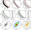 |
Fig. 2. Illustration of the selection procedures we applied to isolate MSa stars. (a) Preliminary selection of MSa candidates on the mF336W − mF438W CMD (within the red lines). (b)-(c) Selection refinements using two CMDs of different colours. We show MSa stars selected from the previous panel in black and, the rest of the MS in grey. Rejected stars are those outside the two red lines. (d) Fiducial lines (in green) used to verticalise the MSa in the mF336W − mF438W CMD. Stars that survived the selections from panels (a)+(b)+(c) are represented in black, while other stars are in grey. (e) Verticalised |

The corresponding procedures for fields F5, F3, and F2 are shown in Figs. A.1, A.2 and A.3 of the Appendix, respectively. Because of the limited number of stars in field F1, the MSa sequence was not identifiable, and therefore we omitted the MSa analysis for this field. The TpCD obtained for field F5 closely resembles that of field F4, albeit with a slightly more blurred appearance due to the lower photometric quality of field F5. Similarly, the TpCDs obtained for fields F2 and F3 exhibit a similar pattern, but the limited number of stars in these fields, particularly belonging to the MSa populations, results in low statistical significance. As a result, a reliable separation of the two stellar populations is not feasible in these fields, and therefore only the total number of MSa stars in these two fields was considered. The final sample of MSa stars in fields F2 and F3 consists of those falling inside the black envelope in panel (l) of Figs. A.3 and A.2, respectively, which are represented by black dots.
4.2. bMS
The bMS stands out distinctly on the blue side of the MS, rendering it easily distinguishable. This is evident in panel (a) of Fig. 3, which illustrates the mF438W − mF814W CMD. This is the most populous of the chemically anomalous 2P groups (see Table 1 of Bellini et al. 2017c) and corresponds to a population with significant enrichment in light elements such as helium and nitrogen. In this and the following panels of the figure, all previously identified stars (in this case, MSa1 and MSa2 stars) have been removed. The two red lines delineate the colour boundaries of our preliminarily selected bMS stars. The selection is confined to the magnitude range 20.16 < mF438W < 22.36, as indicated by the two horizontal red lines. In panel (b), we show the mF336W − mF438W CMD of preliminarily selected bMS stars from panel (a). Stars rejected in panel (a) are in grey. We removed a few outliers using the two red lines. A further selection refinement is applied on the mF275W − mF438W CMD (panel (c)). The mF336W − mF438W and mF275W − mF336W CMDs of the stars surviving all the selections are represented in black in panels (d) and (f), respectively, while the excluded stars are shown in grey. The green fiducial lines are used to verticalise the sequences of bMS stars following the same procedure as that used above for the MSa. The two verticalised  and
and  CMDs are shown in panels (e) and (g). Panel (h) shows the
  versus
  TpCD of the bMS stars, while the Hess diagram of the TpCD is presented in panel (i). The TpCDs presented in panels (h) and (i) closely resemble those illustrated in Bellini et al. (2017c, see Fig. 2) in terms of its shape. Consistent with the findings in Bellini et al. (2017c), we can distinctly identify three stellar populations, each characterised by clumps located at coordinates (0.3, 0.3), (0.5, 0.6), and (0.8, 0.8). It is worth noting that the clump situated at (0.5, 0.6) appears to be more prominent and visually discernible compared to the findings reported in Bellini et al. (2017c), suggesting a possible radial gradient within the bMS subpopulations. However, it is evident that all clumps display varying degrees of overlap and contamination with each other, and their structure appears highly fragmented. Following the same approach as Bellini et al. (2017c), we defined three subpopulations of the bMS in panel (l): the bMS1 (blue), the bMS2 (azure), and the bMS3 (cyan), each defined as all stars within the respective black envelope.
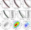 |
Fig. 3. Similar to Fig. 2 but for the bMS stars. (a) Preliminary selection of bMS stars on the mF438W − mF814W CMD (within the red lines). Already identified MSa1 and MSa2 stars have been removed from the CMD. (b)-(c) Preliminarily selected bMS stars are further refined using the mF336W − mF438W and mF275W − mF438W CMDs. As for Fig. 2, stars surviving from the previous panel are in black, while rejected stars are in grey. (d)-(f) Fiducial lines (in green) used to verticalise the MSa in the mF336W − mF438W and mF275W − mF336W CMDs. (e)-(g) Verticalised |


The procedures for identifying the bMS population in fields F5, F3, F2, and F1 are outlined in Figs. A.4, A.5, A.6 and A.7 of the Appendix, respectively. Despite variations in photometric accuracy and statistical limitations, the general shape of the TpCDs remains consistent across all fields. In field F5, the TpCD resembles that of field F4, albeit slightly more blurred due to lower photometric accuracy. Given this limitation, we opted not to separate the three subpopulations but to consider only the total number of bMS stars for this field.
In fields F1, F2, and F3, the visibility of the three clumps on the TpCD is reduced due to limited statistics. Nevertheless, in the TpCD in field F2, we recognize a pattern similar to the TpCD in field F4, with three distinct clumps located around coordinates (0.3, 0.3), (0.55, 0.55), and (0.85, 0.85). Notably, the central clump appears even more prominent compared to field F4, which aligns with the earlier anticipation of a potential radial gradient within the bMS subpopulations.
Similar to field F2, in field F1, we can also barely discern three clumps, which might correspond to the three clumps identified in field F4. These clumps have coordinates (0.15, 0.25), (0.55, 0.45), and (0.95, 0.95), with the central clump appearing more prominent once again.
The field F3 presents a challenging scenario in the TpCD analysis. The bMS1 populations appear to be absent, while there is a possible indication of an increase in the populations of bMS2 and bMS3. However, the positions of the three subpopulations in the TpCD are not clearly defined and a reliable separation is not feasible. In spite of these considerations, we attempted to identify the three bMS subpopulations in fields F1 and F2 (see panel (l) of Figs. A.6 and A.7, respectively), while we only considered the total number of bMS stars for field F3. The final sample of bMS stars in fields F5 and F3 consists of those falling inside the black envelope in panel (l) of Figs. A.4 and A.5, respectively, which are represented by black dots.
4.3. rMS
Another straightforward population to isolate is the rMS. Following Bellini et al. (2017c), we consider this our reference 1P group (although it might include two subgroups of stars with a mild nitrogen enhancement; see Table 1 of Bellini et al. 2017c). This population becomes apparent in the mF275W − mF814W CMD shown in panel (a) of Fig. 4, after the removal of MSa and bMS stars. We kept the same magnitude limits as for the bMS, and preliminarily selected rMS stars on this panel by means of the two red lines. Selected stars are then plotted in black in the mF606W − mF814W CMD of panel (b), where we remove a few outliers. An additional rejection of likely outliers is performed on the mF336W − mF438W CMD of panel (c). We verticalised the sequences of rMS stars on the mF336W − mF438W and mF275W − mF336W CMDs by means of the green fiducials shown in panels (d) and (f). The two verticalised  and
and  CMDs are shown in panels (e) and (g). Panel (h) shows the
  versus
  TpCD of selected rMS stars (in black). The corresponding Hess diagram is in panel (i). The shape of the TpCDs presented in panels (h) and (i) resembles those reported by Bellini et al. (2017c, see Fig. 3). Similar to the findings in Bellini et al. (2017c), we can distinguish three distinct stellar populations, characterised by clumps located at coordinates (0.35, 0.65), (0.65, 0.45), and (0.8, 0.3). However, it is important to note that all clumps exhibit a higher degree of overlap and contamination compared to the results reported by Bellini et al. (2017c). The shape of these clumps and the relative abundance of their populations appear slightly different from the findings of Bellini et al. (2017c). Specifically, the leftmost clumps appear more prominent than those observed in this latter study. This variation could be attributed to contamination by other populations, such as the populations MSe (discussed in Section 4.5), or it could indicate intrinsic variations in the number of stars within the rMS subpopulations as a function of radial distance from the cluster centre. Following the approach of Bellini et al. (2017c) we defined three rMS subpopulations in panel (l): rMS1 (brown), rMS2 (red), and rMS3 (orange).
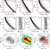 |
Fig. 4. Similar to Figs. 2 and 3 but for the rMs stars. The Hess diagram in panel (i) reveals three main subcomponents, labelled rMS1 (brown), rMS2 (red), and rMS3 (orange) in panel (l). |
Corresponding figures for the other fields are presented in Figs. A.8, A.9, A.10 and A.11 of the Appendix. Across all fields, the general shape of the TpCDs remains consistent. In field F5, the TpCD resembles that of field F4, yet it is significantly blurred, hindering accurate identification of the three subpopulations. In fields F1, F2, and F3, only the leftmost clump is clearly visible, appearing more prominent compared to fields F4 and F5, particularly in field F3. The other two clumps are barely discernible, posing challenges for identification. Similar to fields F4 and F5, the dominance of the leftmost clump in fields F1, F2, and F3 might stem from contamination by other populations or intrinsic radial variations in the number of stars within the three rMS subpopulations. As a result, we opted not to estimate any subpopulations for these fields, and only consider the total number of rMS stars. The final sample of rMS stars in these fields consists of those falling inside the black envelope in panel (l) of Figs. A.8, A.9, A.10 and A.11, which are represented by black dots.
4.4. MSd
Here, we turn our focus to the MSd population (see Bellini et al. 2017c). According to the study of Bellini et al. (2017c), the chemical properties of this 2P subgroup would be characterised by Fe and helium enhancement (less extreme than the MSa population discussed in Section 4.1) and a modest nitrogen enhancement compared to the reference rMS population. In panel (a) of Fig. 5, we present the mF336W − mF814W CMD for stars not categorised under populations MSa, bMS, and rMS. We selected all stars falling between the two red diagonal lines and kept the same magnitude limits used for the bMS and rMS stars (red horizontal lines). Panel (b) shows the mF606W − mF814W CMD of these selected stars in black, where two distinct sequences are evident. The MSd stars, situated in the blue component, are preliminarily selected (red lines) in panel (b). Further refinement of the MSd sample involved removing a few outliers using the mF275W − mF814W and mF336W − mF438W CMDs (panels (c) and (d), respectively). The fiducials used to verticalise the MSd sequence in the mF336W − mF438W and mF275W − mF336W CMDs are shown in green in panels (e) and (g), while the verticalised  and
and  CMDs are shown in panels (f) and (h). The TpCD and Hess diagrams of selected MSd stars are shown in panels (i) and (l), respectively. The TpCD shape resembles that presented in Bellini et al.(2017c, see Fig. 5), where three clumps were identified: two primary clumps situated in the lower-left and centre sections of the plot, and a less populated clump positioned in the upper-right section. Similarly, we observe two main clumps at coordinates (0.25, 0.3) and (0.6, 0.65), along with a less populated clump at (0.8, 0.85). However, the two main clumps exhibit significant overlap and contamination, posing a challenge for clear subpopulation separation. The border between these clumps appears higher and more towards the right than what was presented in Bellini et al. (2017c), with the (0.25, 0.3) clump appearing more prominent compared to the findings reported by these latter authors. The three subpopulations are defined in panel (m), labelled MSd1 (pink), MSd2 (magenta), and MSd3 (purple).
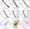 |
Fig. 5. (a) mF336W − mF814W CMD of the MS stars not belonging to MSa, bMs, or rMS. We selected all stars falling between the two red diagonal lines. (b) mF606W − mF814W CMD of the stars selected in (a), where they clearly split into two components. The MSd stars, situated in the blue component, are preliminarily selected. (c)-(d) Selection refinements for MSd stars. (e)-(g) Fiducials (in green) used to verticalise the MSd sequence in the mF336W − mF438W and mF275W − mF336W CMDs. (f)-(h) Verticalised |


The TpCD for field F5 (see Fig. A.12) presents a challenging scenario for the identification of the three subpopulations, displaying a different structure compared to what was obtained for field F4. Additionally, the TpCDs for fields F3, F2, and F1 (see Figs. A.13, A.14 and A.15, respectively) are characterised by a low number of stars and poor statistics, making it very difficult to identify the three clumps. Due to these limitations, we decided not to apply any subpopulation selection for these fields, but to only consider the total number of MSd stars. The final sample of MSd stars in these fields consists of those falling inside the black envelope in panel (m) of Figs. A.12, A.13, A.14 and A.15, which are represented by black dots.
4.5. MSe
Here, we focus our attention on the red component, constituting the MSe population (see Bellini et al. 2017c), which was excluded in panel (b) of Fig. 5. This population is composed of various subpopulations with chemical abundances slightly enhanced in Fe and/or nitrogen relative to the rMS population (see Bellini et al. 2017c). Panel (a) of Fig. 6 is similar to panel (b) of Fig. 5, but without MSd stars. Within this panel, we initially selected MSe stars as those enclosed by the two red lines. We refined the MSe sample as shown in panels (b) and (c). Panels (d) and (f) of Fig. 6 show the fiducials used to verticalise the MSe sequence, while panels (e) and (g) exhibit the verticalised CMDs. Panels (h) and (i) show the TpCD of the selected MSe stars and the corresponding Hess diagram. The TpCD presented here closely resembles that illustrated in Bellini et al. (2017c, see Fig. 6): two prominent clumps are clearly discernible, situated at approximately (0.45, 0.3) and (0.25, 0.75). However, due to lower statistics, the identification of the additional two less populated clumps introduced by Bellini et al. (2017c) is not feasible. Therefore, we focus our attention on the two main clumps. In panel (l), we consequently delineate the following two MSe subpopulations: MSe1 (lime) and MSe2 (green).
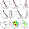 |
Fig. 6. (a) Same as panel (b) of Fig. 5, but MSd stars are also removed. The remaining stars, constituting the MSe population, form a well-defined sequence on this plane, which we select and further refine in panels (b) and (c). (d)-(f) Fiducials (in green) used to verticalise the MSe sequences. (e)-(g) Verticalised CMDs. (h)-(i) TpCD and the Hess diagram of MSe stars. (l) We identified the two MSe populations as MSe1 (lime) and MSe2 (green). |
The corresponding figures for fields F5, F3, F2, and F1 are presented in Figs. A.16, A.17, A.18 and A.19, respectively. For field F5, the obtained TpCD closely resembles that of field F4, albeit more blurred. In fields F2 and F3, despite lower statistics, we are still able to identify the two subpopulations. However, in field F1, the two subpopulations are not discernible, and so we only consider the total number of MSe stars in this field.
5. Radial variation among stellar populations
Table A.1 presents the count and relative percentage of stars in the magnitude range 20.16 < mF438W < 22.36, across the five identified mPOPs and their subpopulations, alongside the estimated number of unidentified stars5 in fields F1, F2, F3, F4, and F5. Errors are estimated using Poisson errors and by propagating the uncertainties. For convenience, the corresponding values from the central field reported by Bellini et al. (2017c) are also included in Table A.1. The distance interval from the cluster centre is provided for each field, with the fields listed in order from the closest to the farthest. The fractions of stars in each main population for each field are also illustrated in Fig. 7 as a function of radial distance from the cluster centre.
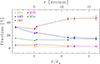 |
Fig. 7. Fractions of stars in each main population for each field as a function of radial distance from the cluster centre, with each population colour coded as indicated in the top-left corner of the plot. |
The separation and identification of mPOPs, particularly their subpopulations, have proven to be more challenging than outlined in Bellini et al. (2017c). This difficulty stems from lower photometric accuracy and precision, which is attributed to fewer exposures (especially in field F5) and limited star counts and statistics; this is particularly evident in the three outer fields, F1, F2, and F3. Notably, the proportion of unidentified stars in our fields exceeds that reported for the central field (10.34% ± 0.17%), with the highest proportion observed in field F5 (27.84% ± 0.59%). This discrepancy is primarily due to the reduced photometric accuracy in this field. To account for the different photometric quality among the analysed fields and the varying numbers of unidentified stars in each, we also provide in Table A.1, within parentheses, ratios obtained solely from the counts of classified stars.
In all the fields analysed, the two most populous stellar populations observed are the rMS and the bMS populations, except for fields F1 and F3, where the MSe populations outnumber the bMS population. The fraction of MSa stars is approximately constant over the range of radial distances from the cluster centre we have explored, although there is a possible subtle indication of a slight decrease in the outermost regions: the fraction of MSa stars varies from 3.53% ± 0.10% to ∼2.4% in the intermediate (F4 and F5) and ∼1.7% in the outer (F2 and F3) fields. A similar trend is observed when considering only classified stars. The two MSa subpopulations (MSa1 and MSa2) can be separated only in the central and the two intermediate fields. In that radial range, the two populations follow a trend similar to that found for the entire MSa population with no strong indication of a variation in the relative number of stars in each of the two groups.
A clear trend is observed in the bMS population with radial distance from the cluster centre, with bMS populations decreasing from the centre to the outskirts. Specifically, there is a central value of 32.32% ± 0.33%, dropping to ∼23–24% in the two intermediate fields (F4 and F5), and further to ∼14–16% in the three outer fields (F1, F2 and F3). Similar considerations are also valid when considering only classified stars, although the radial variation appears less steep. A reliable division of the three bMS subpopulations was feasible only in the central field and fields F4, F2, and F1. The results obtained from the analysis of these fields show that the fraction of stars in each of these subpopulations follows a radial gradient similar to that found in the total bMS population and decreases at larger distances from the cluster centre. Such a trend, however, appears milder in the bMS2 subpopulation.
The fraction of the total number of stars in the rMS group follows a variation with the distance from the cluster centre that is characterised by an approximately constant fraction in the inner regions and an increasing fraction in the outer regions, a behaviour complementary to that of the other dominant population (the bMS population). This increase becomes more pronounced when considering only classified stars. We note that, as anticipated in Section 4.3, the leftmost clump in the TpCDs for the fields F5, F4, F3, F2, and F1 presents a prominence more evident with respect to what was found in the central field (see Fig. 3 of Bellini et al. 2017c). This can be due to contamination from other populations, especially the MSe populations, which partially overlap the rMS population in most CMDs, or can indicate a radial gradient within the rMS subpopulations. The only field in which we are able to separate the rMS subpopulations with sufficient accuracy is the F4 field. The identification of the three rMS subgroups is possible only in the central field and in the F4 field, making the study of the radial variation of the fraction of stars in the three groups difficult. The data available suggest that the fraction of the total number of rMS belonging to the rMS1 (rMS3) group increases (decreases) with the distance from the cluster centre, while it is approximately constant for the rMS2 group.
For the MSd population, the number of MSd stars in the two intermediate fields (4.68% ± 0.24% and 5.80% ± 0.29% for F5 and F4, respectively) aligns closely with the central field value (5.10% ± 0.12%) but slightly decreases in the two outer fields (3.50% ± 0.54%, 3.23% ± 0.50% and 2.67% ± 0.82% for F2, F3 and F1, respectively). However, when considering only classified stars, we observe a slight increase in the two intermediate fields (6.49% ± 0.33% and 7.31% ± 0.37% for F5 and F4, respectively) with respect to the central value (5.69% ± 0.13%), followed by a decrease in the outer fields (4.38% ± 0.68%, 3.85% ± 0.60% and 3.35% ± 1.03% for F2, F3, and F1, respectively). Among these fields, only field F4 allowed the separation of the MSd subpopulations, although with considerable uncertainties due to the envelope positions in the TpCD. Nonetheless, the number counts suggest a potential trend among the MSd subpopulations. While the fraction of the total number of MSd stars in the MSd3 group remains relatively constant in the central field and field F4 (∼0.20–0.22), the fraction of MSd stars in the MSd1 and MSd2 subpopulations exhibits a radial gradient. Specifically, from the central field to field F4, the MSd1/MSd ratio increases from MSd1/MSd∼0.38 ± 0.02 to MSd1/MSd∼0.56 ± 0.05 (an increase of ∼68%), while the MSd2/MSd ratio decreases from MSd2/MSd∼0.41 ± 0.02 to MSd2/MSd∼0.24 ± 0.03 (a decrease of ∼60%). However, it is important to note that these numbers are affected by uncertainties stemming from the envelope positions on the TpCD, as mentioned above.
For the MSe population, the number of stars remains relatively stable across varying radial distances from the cluster centre, ranging between ∼13.8% and 17.2%. When considering only classified stars, we observe a consistent ratio in the central field and fields F5, F4, and F2 (∼16–17%) and then a slight increase in the outermost fields, F3 and F1 (∼20%). Although we were unable to separate the smallest MSe subpopulations (MSe3 and MSe4) due to low statistics, we achieved accurate separation of the two main MSe subpopulations (MSe1 and MSe2) in fields F2, F3, F4, and F5. The relative number of the two subpopulations, MSe1 and MSe2, maintains a constant ratio in the central field and in the intermediate fields (F4 and F5), with MSe2/MSe1 ∼1, while it shows a notable increase in the two outer fields (F2 and F3), with a value of MSe2/MSe1 ∼2.2.
As outlined in Section 1, Bellini et al. (2009) conducted an extensive examination of the radial distribution of the two primary stellar populations in ω Cen (rMs and bMS), identifying a radial gradient in their number-count fraction (bMS/rMS). In Fig. 8, we show a comparison with the radial profile presented in Bellini et al. (2009, black points) alongside the ratios derived from the data presented in this study (red points) and in Bellini et al. (blue point 2017c), revealing a notable agreement between the datasets.
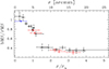 |
Fig. 8. bMS/rMS as a function of radial distance. Black points represent data from Bellini et al. (2009), the blue point is from Bellini et al. (2017c), and the red points are from the present study. |
6. Summary
In this paper, we present the reduction process of HST data acquired through the GO-16247 (P.I.: Scalco) and GO-14118+14662 (P.I.: Bedin) programmes. We provide an overview of the dataset and the process of data reduction. We combined the newly obtained data with previously processed data (see Scalco et al. 2021) to extend the analysis of Bellini et al. (2017c), thus presenting, for the first time, a comprehensive investigation of the radial gradient of the mPOPs within ω Cen spanning a significant portion of the cluster.
Our analysis reveals significant radial variations in the fraction of stars in the stellar populations of ω Cen and their subpopulations. For the two dominant populations, the bMS and the rMS, our results show that the fraction of bMS (rMS) decreases (increases) with the distance from the cluster centre. Our findings are consistent with those reported by Bellini et al. (2009).
As discussed in Section 1, according to various formation scenarios (see e.g. D’Ercole et al. 2008; Bekki 2010, 2011; Calura et al. 2019), the formation of 2P stars is expected to be more centrally concentrated in the cluster’s inner regions, with 2P stars gradually mixing with 1P stars during the cluster’s evolution. ω Cen has a long relaxation time (∼1.1 Gyr in the core and ∼10 Gyr at the half-mass radius, Harris 1996, 2010), suggesting that the effects of two-body relaxation should not have completely erased the spatial differences imprinted by the formation processes and some ‘memory’ of those differences should still be present in the current properties. This is consistent with our observations: we find that the main 2P population (represented by the bMS population) is more centrally concentrated compared to the 1P population (represented by the rMS population).
It is important to emphasise that the variety of stellar populations and subpopulations hosted by ω Cen is a clear indication of a complex formation history. Interpretation of the differences in the spatial variations requires particular attention and caution. Spectroscopic follow-up studies – of the already characterised stars in this work – are essential for an accurate classification of the chemical properties of these stellar populations in order to gain a deeper understanding of their characteristics. Additionally, the complex formation history and intricate system of stellar populations in ω Cen further underscore the need for future theoretical simulations involving mPOPs – beyond just 1P and 2P – to enhance our understanding of the presented results. Some initial theoretical studies in this direction have been presented by Bekki & Tsujimoto (2019), Lacchin et al. (2021) and Lacchin et al. (2022) and have shown that more extreme 2P stars (i.e. those with higher helium content) may form in an initially more concentrated way than the 2P stars with lower helium content (see also Simioni et al. 2016, for a similar trend in NGC 2808). The much weaker radial variation of the MSd and MSe populations might be consistent with those predictions, but we reiterate the importance of caution in this comparison and recognise the necessity for further observational efforts – to characterise the chemical properties of all the populations – and further theoretical studies before drawing more definitive conclusions.
Finally, we point out that ongoing (such as Euclid) and recently approved – by NASA (e.g. UVEX) – wide-field missions will contribute to the statistical analysis of these stellar populations and to the elucidation of their spatial distribution.
The Appendix of the paper can be found on Zenodo https://zenodo.org/doi/10.5281/zenodo.11490583
The count of unidentified stars in our analysis also includes binaries. In contrast to Bellini et al. (2017c), this study does not provide an estimate of the number of binaries. The decision to neglect the presence of binaries stems from uncertainties and their relatively low abundance in this cluster, as noted in previous studies (see Marks et al. 2022; Wragg 2023).
Acknowledgments
Michele Scalco and Luigi Rolly Bedin acknowledge support by MIUR under the PRIN-2017 programme #2017Z2HSMF, and by INAF under the PRIN-2019 programme #10-Bedin.
References
- Anderson, J. 2016, Empirical Models for the WFC3/IR PSF, Instrument Science Report WFC3 2016-12, 42 [Google Scholar]
- Anderson, J. 2022, One-Pass HST Photometry with hst1pass, Instrument Science Report WFC3 2022-5, 55 [Google Scholar]
- Anderson, J., & King, I. R. 2000, PASP, 112, 1360 [NASA ADS] [CrossRef] [Google Scholar]
- Anderson, J., & King, I. R. 2006, PSFs, Photometry, and Astronomy for the ACS/WFC, Instrument Science Report ACS 2006-01, 34 [Google Scholar]
- Anderson, J., Sarajedini, A., Bedin, L. R., et al. 2008, AJ, 135, 2055 [Google Scholar]
- Balaguer-Núnez, L., Tian, K. P., & Zhao, J. L. 1998, A&AS, 133, 387 [Google Scholar]
- Bastian, N., & Lardo, C. 2018, ARA&A, 56, 83 [Google Scholar]
- Bedin, L. R., Piotto, G., Anderson, J., et al. 2004, ApJ, 605, L125 [Google Scholar]
- Bedin, L. R., Cassisi, S., Castelli, F., et al. 2005, MNRAS, 357, 1038 [NASA ADS] [CrossRef] [Google Scholar]
- Bedin, L. R., King, I. R., Anderson, J., et al. 2008, ApJ, 678, 1279 [NASA ADS] [CrossRef] [Google Scholar]
- Bekki, K. 2010, ApJ, 724, L99 [CrossRef] [Google Scholar]
- Bekki, K. 2011, MNRAS, 412, 2241 [NASA ADS] [CrossRef] [Google Scholar]
- Bekki, K., & Freeman, K. C. 2003, MNRAS, 346, L11 [Google Scholar]
- Bekki, K., & Norris, J. E. 2006, ApJ, 637, L109 [NASA ADS] [CrossRef] [Google Scholar]
- Bekki, K., & Tsujimoto, T. 2019, ApJ, 886, 121 [NASA ADS] [CrossRef] [Google Scholar]
- Bellini, A., Piotto, G., Bedin, L. R., et al. 2009, A&A, 493, 959 [NASA ADS] [CrossRef] [EDP Sciences] [Google Scholar]
- Bellini, A., Bedin, L. R., Piotto, G., et al. 2010, AJ, 140, 631 [NASA ADS] [CrossRef] [Google Scholar]
- Bellini, A., Anderson, J., & Bedin, L. R. 2011, PASP, 123, 622 [CrossRef] [Google Scholar]
- Bellini, A., Anderson, J., van der Marel, R. P., et al. 2014, ApJ, 797, 115 [Google Scholar]
- Bellini, A., Anderson, J., Bedin, L. R., et al. 2017a, ApJ, 842, 6 [NASA ADS] [CrossRef] [Google Scholar]
- Bellini, A., Anderson, J., van der Marel, R. P., et al. 2017b, ApJ, 842, 7 [NASA ADS] [CrossRef] [Google Scholar]
- Bellini, A., Milone, A. P., Anderson, J., et al. 2017c, ApJ, 844, 164 [NASA ADS] [CrossRef] [Google Scholar]
- Bellini, A., Libralato, M., Bedin, L. R., et al. 2018, ApJ, 853, 86 [NASA ADS] [CrossRef] [Google Scholar]
- Calamida, A., Zocchi, A., Bono, G., et al. 2020, ApJ, 891, 167 [Google Scholar]
- Calura, F., D’Ercole, A., Vesperini, E., Vanzella, E., & Sollima, A. 2019, MNRAS, 489, 3269 [Google Scholar]
- D’Ercole, A., Vesperini, E., D’Antona, F., McMillan, S. L. W., & Recchi, S. 2008, MNRAS, 391, 825 [CrossRef] [Google Scholar]
- Gaia Collaboration (Brown, A. G. A., et al.) 2016, A&A, 595, A2 [NASA ADS] [CrossRef] [EDP Sciences] [Google Scholar]
- Gaia Collaboration (Vallenari, A., et al.) 2023, A&A, 674, A1 [NASA ADS] [CrossRef] [EDP Sciences] [Google Scholar]
- Gerasimov, R., Burgasser, A. J., Homeier, D., et al. 2022, ApJ, 930, 24 [NASA ADS] [CrossRef] [Google Scholar]
- Gratton, R., Bragaglia, A., Carretta, E., et al. 2019, A&ARv, 27, 8 [Google Scholar]
- Harris, W. E. 1996, AJ, 112, 1487 [Google Scholar]
- Harris, W. E. 2010, ArXiv e-prints [arXiv:1012.3224] [Google Scholar]
- Ibata, R. A., Bellazzini, M., Malhan, K., Martin, N., & Bianchini, P. 2019, Nat. Astron., 3, 667 [Google Scholar]
- Jurcsik, J. 1998, ApJ, 506, L113 [CrossRef] [Google Scholar]
- King, I. R., Bedin, L. R., Cassisi, S., et al. 2012, AJ, 144, 5 [NASA ADS] [CrossRef] [Google Scholar]
- Lacchin, E., Calura, F., & Vesperini, E. 2021, MNRAS, 506, 5951 [NASA ADS] [CrossRef] [Google Scholar]
- Lacchin, E., Calura, F., Vesperini, E., & Mastrobuono-Battisti, A. 2022, MNRAS, 517, 1171 [NASA ADS] [CrossRef] [Google Scholar]
- Latour, M., Calamida, A., Husser, T. O., et al. 2021, A&A, 653, L8 [NASA ADS] [CrossRef] [EDP Sciences] [Google Scholar]
- Libralato, M., Bellini, A., Bedin, L. R., et al. 2018, ApJ, 854, 45 [NASA ADS] [CrossRef] [Google Scholar]
- Libralato, M., Bellini, A., Vesperini, E., et al. 2022, ApJ, 934, 150 [NASA ADS] [CrossRef] [Google Scholar]
- Marks, M., Kroupa, P., & Dabringhausen, J. 2022, A&A, 659, A96 [NASA ADS] [CrossRef] [EDP Sciences] [Google Scholar]
- Milone, A. P., Piotto, G., Bedin, L. R., et al. 2012, A&A, 540, A16 [NASA ADS] [CrossRef] [EDP Sciences] [Google Scholar]
- Milone, A. P., Marino, A. F., Piotto, G., et al. 2015a, MNRAS, 447, 927 [NASA ADS] [CrossRef] [Google Scholar]
- Milone, A. P., Marino, A. F., Piotto, G., et al. 2015b, ApJ, 808, 51 [NASA ADS] [CrossRef] [Google Scholar]
- Milone, A. P., Marino, A. F., Bedin, L. R., et al. 2017, MNRAS, 469, 800 [NASA ADS] [CrossRef] [Google Scholar]
- Nardiello, D., Libralato, M., Piotto, G., et al. 2018, MNRAS, 481, 3382 [NASA ADS] [CrossRef] [Google Scholar]
- Norris, J. E. 2004, ApJ, 612, L25 [NASA ADS] [CrossRef] [Google Scholar]
- Norris, J. E., Freeman, K. C., Mayor, M., & Seitzer, P. 1997, ApJ, 487, L187 [NASA ADS] [CrossRef] [Google Scholar]
- Pancino, E., Ferraro, F. R., Bellazzini, M., Piotto, G., & Zoccali, M. 2000, ApJ, 534, L83 [NASA ADS] [CrossRef] [Google Scholar]
- Renzini, A., D’Antona, F., Cassisi, S., et al. 2015, MNRAS, 454, 4197 [Google Scholar]
- Sarajedini, A., Bedin, L. R., Chaboyer, B., et al. 2007, AJ, 133, 1658 [Google Scholar]
- Scalco, M., Bellini, A., Bedin, L. R., et al. 2021, MNRAS, 505, 3549 [NASA ADS] [CrossRef] [Google Scholar]
- Simioni, M., Milone, A. P., Bedin, L. R., et al. 2016, MNRAS, 463, 449 [NASA ADS] [CrossRef] [Google Scholar]
- Smith, G. H. 1987, PASP, 99, 67 [Google Scholar]
- Sollima, A., Ferraro, F. R., Bellazzini, M., et al. 2007, ApJ, 654, 915 [NASA ADS] [CrossRef] [Google Scholar]
- van de Ven, G., van den Bosch, R. C. E., Verolme, E. K., & de Zeeuw, P. T. 2006, A&A, 445, 513 [NASA ADS] [CrossRef] [EDP Sciences] [Google Scholar]
- Wragg, F. 2023, in Two in a Million - The Interplay Between Binaries and Star Clusters, 12 [Google Scholar]
Appendix A: Additional table
Distribution of stars among various populations in the analysed fields.
All Tables
All Figures
|
Fig. 1. Outlines of the fields observed in HST programs GO-14118+14662 (P.I.: Bedin) and GO-16427 (P.I.: Scalco), superimposed on a DSS image of ω Cen. The primary GO-14118+14662 field (F0) is shown in blue, while the three GO-14118+14662 parallel WFC3 fields are shown in pink. The two GO-16427 fields are shown in green. The data discussed in this paper come from fields F2, F3, F4, and F5. We also show the central field from Bellini et al. (2017a,b,c) in yellow. Units are in arcminutes measured from the cluster centre. The white dashed circle marks the rc while the red dashed circles mark the half-light radius (rh = 5.00 arcmin; from Harris 1996, 2010), and 2 rh and 3 rh from the centre. |
| In the text | |
|
Fig. 2. Illustration of the selection procedures we applied to isolate MSa stars. (a) Preliminary selection of MSa candidates on the mF336W − mF438W CMD (within the red lines). (b)-(c) Selection refinements using two CMDs of different colours. We show MSa stars selected from the previous panel in black and, the rest of the MS in grey. Rejected stars are those outside the two red lines. (d) Fiducial lines (in green) used to verticalise the MSa in the mF336W − mF438W CMD. Stars that survived the selections from panels (a)+(b)+(c) are represented in black, while other stars are in grey. (e) Verticalised |
| In the text | |
|
Fig. 3. Similar to Fig. 2 but for the bMS stars. (a) Preliminary selection of bMS stars on the mF438W − mF814W CMD (within the red lines). Already identified MSa1 and MSa2 stars have been removed from the CMD. (b)-(c) Preliminarily selected bMS stars are further refined using the mF336W − mF438W and mF275W − mF438W CMDs. As for Fig. 2, stars surviving from the previous panel are in black, while rejected stars are in grey. (d)-(f) Fiducial lines (in green) used to verticalise the MSa in the mF336W − mF438W and mF275W − mF336W CMDs. (e)-(g) Verticalised |
| In the text | |
|
Fig. 4. Similar to Figs. 2 and 3 but for the rMs stars. The Hess diagram in panel (i) reveals three main subcomponents, labelled rMS1 (brown), rMS2 (red), and rMS3 (orange) in panel (l). |
| In the text | |
|
Fig. 5. (a) mF336W − mF814W CMD of the MS stars not belonging to MSa, bMs, or rMS. We selected all stars falling between the two red diagonal lines. (b) mF606W − mF814W CMD of the stars selected in (a), where they clearly split into two components. The MSd stars, situated in the blue component, are preliminarily selected. (c)-(d) Selection refinements for MSd stars. (e)-(g) Fiducials (in green) used to verticalise the MSd sequence in the mF336W − mF438W and mF275W − mF336W CMDs. (f)-(h) Verticalised |
| In the text | |
|
Fig. 6. (a) Same as panel (b) of Fig. 5, but MSd stars are also removed. The remaining stars, constituting the MSe population, form a well-defined sequence on this plane, which we select and further refine in panels (b) and (c). (d)-(f) Fiducials (in green) used to verticalise the MSe sequences. (e)-(g) Verticalised CMDs. (h)-(i) TpCD and the Hess diagram of MSe stars. (l) We identified the two MSe populations as MSe1 (lime) and MSe2 (green). |
| In the text | |
|
Fig. 7. Fractions of stars in each main population for each field as a function of radial distance from the cluster centre, with each population colour coded as indicated in the top-left corner of the plot. |
| In the text | |
|
Fig. 8. bMS/rMS as a function of radial distance. Black points represent data from Bellini et al. (2009), the blue point is from Bellini et al. (2017c), and the red points are from the present study. |
| In the text | |
Current usage metrics show cumulative count of Article Views (full-text article views including HTML views, PDF and ePub downloads, according to the available data) and Abstracts Views on Vision4Press platform.
Data correspond to usage on the plateform after 2015. The current usage metrics is available 48-96 hours after online publication and is updated daily on week days.
Initial download of the metrics may take a while.