| Issue |
A&A
Volume 692, December 2024
|
|
|---|---|---|
| Article Number | A135 | |
| Number of page(s) | 8 | |
| Section | Galactic structure, stellar clusters and populations | |
| DOI | https://doi.org/10.1051/0004-6361/202451310 | |
| Published online | 06 December 2024 | |
Hubble Space Telescope survey of Magellanic Cloud star clusters. Binaries among the split main sequences of NGC 1818, NGC 1850, and NGC 2164
1
Dipartimento di Fisica e Astronomia “Galileo Galilei”, Università Degli Studi di Padova,
Vicolo dell’Osservatorio 3,
35122
Padova,
Italy
2
Istituto Nazionale di Astrofisica – Osservatorio Astronomico di Padova,
Vicolo dell’Osservatorio 5,
35122
Padova,
Italy
3
Istituto Nazionale di Astrofisica, Osservatorio Astronomico di Roma,
Via Frascati 33,
00077
Monte Porzio Catone,
Italy
4
Research School of Astronomy and Astrophysics, Australian National University,
Canberra,
ACT 2611,
Australia
5
School of Physics and Astronomy, Sun Yat-sen University,
Zhuhai
519082,
China
6
CSST Science Center for the Guangdong–Hong Kong-Macau Greater Bay Area,
Zhuhai
519082,
PR
China
7
Key Laboratory for Optical Astronomy, National Astronomical Observatories, Chinese Academy of Sciences,
Beijing
100101,
PR
China
8
School of Astronomy and Space Science, University of Chinese Academy of Sciences,
Beijing
100049,
PR
China
9
Department of Astronomy, School of Physics and Astronomy, China West Normal University,
Nanchong
637002,
PR
China
10
South-Western Institute for Astronomy Research, Yunnan University,
Kunming
650500,
PR
China
★ Corresponding author; fabrizio.muratore@studenti.unipd.it
Received:
29
June
2024
Accepted:
30
October
2024
Nearly all star clusters younger than ~600 Myr exhibit extended main sequence turnoffs and split main sequences (MSs) in their color-magnitude diagrams. Works based on both photometry and spectroscopy have clearly demonstrated that the red MS is composed of fast-rotating stars, whereas blue-MS stars are slow rotators. Nevertheless, the mechanism responsible for the formation of stellar populations with varying rotation rates remains a topic of debate. Potential mechanisms proposed for the split MS include binary interactions, the early evolution of pre-MS stars, and the merging of binary systems, but a general consensus has yet to be reached. These formation scenarios predict different fractions of binaries among blue- and red-MS stars. Therefore, studying the binary populations can provide valuable constraints that may help clarify the origins of the split MSs. We used high-precision photometry from the Hubble Space Telescope to study the binaries of three young Magellanic star clusters exhibiting split MSs, namely NGC 1818, NGC 1850, and NGC 2164. By analyzing the photometry in the F225W, F275W, F336W, and F814W filters for observed binaries and comparing it to a large sample of simulated binaries, we determined the fractions of binaries within the red and blue MS. We find that the fractions of binaries among the blue-MS stars are higher than those of red-MS stars by a factor of ~1.5, 4.6, and ~1.9 for NGC 1818, NGC 1850, and NGC 2164, respectively. We discuss these results in the context of the formation scenarios of the split MS.
Key words: binaries: general / stars: rotation / Magellanic Clouds / galaxies: star clusters: general
© The Authors 2024
 Open Access article, published by EDP Sciences, under the terms of the Creative Commons Attribution License (https://creativecommons.org/licenses/by/4.0), which permits unrestricted use, distribution, and reproduction in any medium, provided the original work is properly cited.
This article is published in open access under the Subscribe to Open model. Subscribe to A&A to support open access publication.
1 Introduction
High-precision photometry from the Hubble Space Telescope (HST) and ground-based observatories have shown that the color-magnitude diagrams (CMDs) of Magellanic Cloud star clusters younger than approximately two billion years are complex and cannot be explained by simple isochrones (see Milone & Marino 2022; Li et al. 2024, for recent reviews). The CMDs of nearly all clusters younger than 600 Myr exhibit extended main-sequence turnoffs (eMSTOs) and split main sequences (MSs; Milone et al. 2015, 2018; D’Antona et al. 2015), with the reddest sequence being the most populated. In contrast, the star clusters with ages between ~600 Myr and ~2 Gyr show only the eMSTO (e.g., Bertelli et al. 2003; Mackey & Broby Nielsen 2007; Glatt et al. 2008; Milone et al. 2009; Goudfrooij et al. 2011; Correnti et al. 2014).
Nowadays, it is widely accepted that stellar rotation plays a major role in shaping the split MSs and eMSTOs of young and intermediate-age star clusters (Bastian & de Mink 2009; D’Antona et al. 2015; Niederhofer et al. 2015; Cordoni et al. 2018; Georgy et al. 2019). However, in addition to the rotation, factors such as age spread and dust have also been proposed as potential contributors to the observed eMSTOs (see Goudfrooij et al. 2017; Milone et al. 2017; Li et al. 2017; Cordoni et al. 2022; D’Antona et al. 2023, for a discussion).
The MSs of clusters younger than ~600 Myr host rapidly rotating stars, which compose the red MS (rMS), and a slowly rotating stellar population in the blue MS (bMS). This was first suggested by the comparison between isochrones with different rotation rates and the observed CMDs of clusters with split MSs (D’Antona et al. 2015; Milone et al. 2016) and has since been proven by works based on high-resolution spectra of MS stars (Marino et al. 2018a,b). Similarly, the eMSTO hosts stars with different rotation rates, with fast rotators populating the upper eMSTO (Dupree et al. 2017; Bastian et al. 2018; Cristofari et al. 2024; Cordoni et al. 2024).
The physical reasons behind the presence of both fast-rotating stars and slow rotators in Magellanic Cloud clusters remain unsettled. Observations of field stars in the last century showed that field stars also display a bimodal distribution, especially in the mass range 2.4 to 3.85 M⊙ (Zorec & Royer 2012), with a slow and a fast velocity component. A similar bimodality in the velocity distribution was also detected among early B-type stars by Dufton et al. (2013). Zorec & Royer (2012) suggested two possible reasons for this velocity difference:
The first possibility is based on the fact that it is unlikely that pre-MS stars originate with zero angular momentum. It is possible, however, that a fraction of them could have undergone magnetic braking.
Some form of tidal braking is occurring due to the presence of a stellar companion. This tidal braking may be significantly more efficient than that predicted by the dynamical tidal model proposed by Zahn (1975, 1977). Discussions of this possibility are presented in D’Antona et al. (2015) and He et al. (2023).
These two hypotheses were revived more recently, the first one mainly by Bastian et al. (2020) and the second one by D’Antona et al. (2015, 2017): stars may not be able to accelerate during the pre-MS contraction if they are magnetically locked with the accretion disk, and they can therefore reach the MS with a reduced rotation. As a consequence, the presence of bMS and rMS stars in young star clusters would depend on the early evolution of pre-MS stars, particularly on whether they retain or lose their protoplanetary disks during the first few million years.
The alternative is that interactions in binary star systems are responsible for stellar braking. In this case, tidal interactions would lead to braking effects within the core, extending outward. Stars would only reach their final position on the nonrotating sequence once the braking process extends to the stellar envelope and photosphere. If this occurs, the star would shift to the bMS. D’Antona et al. (2015) adopted this view to interpret the split MS of the Large Magellanic Cloud (LMC) star cluster NGC 1856, quoting the study of A- and B-type binary stars in the Galactic field by Abt & Boonyarak (2004), who found that close binaries with periods between 4 and 500 days rotate significantly more slowly than single stars. This process would lead to a higher binary fraction in slow rotators than in the rapidly rotating population, and the bMS would predominantly consist of binaries with small mass ratios.
Wang et al. (2022) suggested that binary mergers of MS stars could be responsible for generating slow rotators. When the two stars in a binary merge, the outcome is a single star that has a core hydrogen content higher than that of a single star of the same mass and age. As a result, these merger products, despite having the same age as other cluster stars, appear younger and exhibit a bluer color in the CMD. In this case, we would potentially observe a lack of binaries among slow-rotating stars.
Studying binary systems comprising slow- and fast-rotating stars in clusters with split MSs would help constrain formation scenarios of stellar populations with different rotation rates. Pioneering work by Kamann et al. (2021), based on radial velocities and rotational velocities of stars in the LMC cluster NGC 1850, found a comparable fraction of binaries among bMS and rMS stars, 5.9 ± 1.1% and 4.5 ± 0.6%, respectively.
In addition to providing insights into the origins of split MSs and eMSTOs, understanding the binary populations in star clusters is crucial for numerous astrophysical studies. Binaries significantly influence the dynamical evolution of clusters, serving as an important source of heating. Accurate measurements of the binary fraction are necessary for determining the stellar mass and luminosity functions in globular clusters. Moreover, stellar evolution in binary systems can differ from that of isolated stars: it could lead to the formation of unique objects, such as blue stragglers, cataclysmic variables, millisecond pulsars, and low-mass X-ray binaries.
In this work, we used multi-band HST photometry obtained as part of our recent survey of Magellanic Cloud stars clusters (Milone et al. 2023a) to study the binaries in the young LMC clusters NGC 1818 (40 Myr), NGC 1850 (~90 Myr), and NGC 2164 (~100 Myr) and infer the incidence of binaries among bMS and rMS stars. The paper is organized as follows. Section 2 describes the dataset, and Sect. 3 illustrates the methods we used to estimate the fraction of binaries in the bMS and rMS. Finally, Sect. 4 is dedicated to a summary and a discussion of the results.
2 Data
The data used in this work consist of images of NGC 1818, NGC 1850, and NGC 2164 collected with the Ultraviolet and Visual Channel of the Wide Field Camera 3 (UVIS/WFC3) on board HST. Stellar positions and photometry are derived by Milone et al. (2023a,b) as part of their HST survey of Magellanic Cloud star clusters. For NGC 1818 and NGC 2164, we used photometry in the F225W, F336W, and F814W bands of UVIS/WFC3, whereas for NGC 1850 we used F275W, F336W, and F814W stellar magnitudes.
The data reduction was carried out with the KS2, a computer program developed by Jay Anderson. Originally designed to reduce images collected with the Wide Field Channel of the Advanced Camera for Surveys on board the HST, KS2 has evolved from the earlier “kitchen sync” program (Anderson et al. 2008).
In a nutshell, KS2 employs three distinct methods for measuring stars, with each method optimizing astrometry and photometry for stars of varying luminosities. Since our focus is on bright stars, we utilized the results obtained from Method I. This method takes advantage of the best effective point spread function (ePSF) model (Anderson & King 2000) to measure all stellar sources that produce a distinct peak within a 5×5 pixel region, following the subtraction of neighboring stars. It calculates the flux and position of each star in each image separately, by using the ePSF model associated with its position. The sky level is subtracted considering an annulus between four and eight pixels from the stellar center. Finally, the results from all images are averaged to determine the best stellar magnitudes and positions. The photometry was calibrated to the Vega-mag reference frame by using the zero points provided by the Space Telescope Science Institute website.
The KS2 program offers various diagnostics of photometric quality. In our analysis, we focused on isolated stars that are well fitted by the ePSF model. For NGC 1850 we used the stellar proper motions computed by Milone et al. (2023b) by comparing the stellar positions measured in multi-epoch images. These proper motions are used to separate the bulk of field stars from cluster members.
The photometry of NGC 1850 was corrected for the effects of differential reddening by using the reddening maps derived by Milone et al. (2023b). We verified that NGC 1818 and NGC 2173 are not significantly affected by differential reddening by adopting the criteria by Legnardi et al. (2023). Therefore, for these clusters, we used the original photometry. We refer to Sect. 2.4 of Milone et al. (2023a) for further details on the images, the methods for measuring stellar positions and fluxes, and the criteria adopted to select the stars with high-precision photometry and astrometry.
Artificial star tests
For each cluster, we conducted artificial star (AS) tests to estimate photometric errors and generate the simulated CMDs. Following the method outlined by Anderson et al. (2008), we created a list of 20000 ASs. These ASs were designed to mimic the radial distributions and luminosity functions of the observed stars. The instrumental magnitudes of the ASs spanned from approximately −13.6 mag to −9.0 mag in the UVIS/WFC3 F814W filter. For other filters, we derived magnitudes based on the fiducial lines of the rMS and the bMS. To determine the magnitudes and positions of the ASs, we employed the KS2 program, using the same procedure that Milone et al. (2023a) applied to real stars. Our investigation focused exclusively on relatively isolated ASs that exhibited good fits to the point spread function, and that were selected by following the same criteria as those used for the real stars.
In addition to the cluster members, the field of view observed by HST comprises field stars that lie along the same line of sight of each cluster. To minimize the contamination from background and foreground stars, we restricted our analysis to a central field of view, hereafter the cluster field. It was derived by using the procedure from Mohandasan et al. (2024, see their Sect. 3.1). In summary, we estimated the number density of stars brighter than mF336W = 22.0 mag at different radial distances from the cluster center, and identified the radius where the density profile is nearly flat. The portion of the HST field of view outside this radius is dominated by field stars and is named field region. We assumed that the number density of field stars corresponds to the average stellar density in the field region. We defined the radius of the cluster region as the distance at which the observed stellar density is three times higher than the field density. The radii of the cluster and field regions, within we selected cluster members and field stars, are listed in Table 1 for each cluster, whereas the mF336W versus mF336W − mF814W and mF336W versus mF275W − mF336W CMDs for stars in the cluster and reference fields are shown in Fig. 1.
In the case of NGC 1850 we took advantage of stellar proper motions to further minimize the contamination from field stars. Moreover, the proper motions allowed us to identify and exclude from the analysis the bulk of stars in BRHT 5b, which is a young star cluster that lies on the same line of sight as NGC 1850 (see Milone et al. 2023b, for details on the proper motions of stars in the field of view of NGC 1850). In addition, we excluded stars on the west side of NGC 1850; this includes the stellar overdensity NGC 1850A, which is often considered a separate cluster.
3 The incidence of binaries among red-MS and blue-MS stars
In this section we present the procedure used to derive the fractions of binary systems composed of bMS and rMS stars (hereafter bMS and rMS binaries). Our method, based on the approach introduced by Milone et al. (2020) to infer the fraction of binaries stars among the multiple populations of five Galactic globular clusters, consists of three main steps, which we discuss in the following subsections.
Specifically, in Sect. 3.1 we estimate the fraction of bMS and rMS binaries with respect to a sample of binaries with similar luminosity ratios. Section 3.2 details the procedure used to derive the fractions of bMS, rMS, and binary stars. Finally, we combine these results in Sect. 3.3 to determine the fractions of bMS binaries relative to the total number of bMS stars and rMS binaries relative to the total number of rMS stars.
Radii of the cluster field and minimum and maximum radii for the reference fields.
3.1 The fractions of red-MS and blue-MS stars among binaries
Due to the large distance of the LMC, the binaries analyzed in this work are unresolved stellar systems that appear as point-like sources in the CMD. The magnitude of each system is
![$\[m_{b i n}=m_{1}-2.5 ~\log \left(1+\frac{F_{1}}{F_{2}}\right),\]$](/articles/aa/full_html/2024/12/aa51310-24/aa51310-24-eq1.png) (1)
(1)
where m1 is the magnitude of the brightest star and F1 and F2 are the fluxes of the primary and secondary components, respectively. In a simple-population star cluster, a binary system composed of two MS stars with the same luminosity will result in a source ~0.75 mag brighter than each component and the same color. Hence, the equal-luminosity binaries populate a sequence that runs parallel to the MS, but ~0.75 mag brighter. Binaries composed of two MS stars with different luminosities are located in the CMD region between the MS and the equalluminosity binaries sequences and their colors and magnitudes depend on the luminosities of the two components (see Milone et al. 2012a; Mohandasan et al. 2024, and references therein for details). The procedure that we used to estimate the fraction of binaries among bMS and rMS stars is illustrated in Figs. 2 and 3 for NGC 1850 taken as a test case. The method takes advantage of the mF336W versus mF336W − mF814W CMD, wherein bMS and rMS stars delineate separate sequences. Additionally, it lever-ages the mF336W versus mF275W − mF336W CMD, where the two sequences exhibit considerable overlap.
These CMDs are plotted in Fig. 2, where we use red and blue colors to represent the sample of bona-fide bMS and rMS stars selected by eye from the mF336W versus mF336W − mF814W CMD. The insets of Fig. 2 show the fiducial lines of the rMS and bMS – derived by linearly interpolating the median colors and magnitudes of the selected samples of stars over 0.5 mag wide F336W bins – and the fiducial lines of the equal-luminosity binary sequences – evaluated by subtracting ~0.75 mag from the magnitudes of the rMS and bMS lines.
Our investigation relies on binary systems composed of stars with similar luminosities. As shown in the left panel of Fig. 3, these binaries are selected from the mF336W versus mF275W − mF336W CMD and are situated within the shaded yellow region. Its boundaries were derived as follows. The bright boundary is set at mF336W = 19.6 mag, as for brighter magnitudes binary stars are mixed with MS single stars. The faint boundary is set at mF336W = 20.8 mag because it is challenging to disentangle bMS and rMS binaries with fainter magnitudes. The blue and red limits of the shaded yellow region were obtained by adding and subtracting the corresponding color uncertainties to the colors of the equal-luminosity binary fiducial line. The selected sample comprises 55 candidate binary systems. The selected binaries are marked in the mF336W versus mF336W − mF814W CMD shown in the middle panel of Fig. 3, where the bulk of selected binaries are located near the fiducial lines of equal-luminosity bMS and rMS binaries.
We derived the verticalized mF336W versus ΔF336W,F814W diagram in such a way that the fiducial lines of equal-luminosity binaries are vertical. Specifically, the equal-luminosity bMS fiducial line is set at zero on the abscissa and the one referred to the rMS at one (as illustrated in the top-right panel of Fig. 3).
To minimize the contamination from field stars and stars with large photometric errors (including single stars and binaries with small luminosity ratio), we excluded the outliers with ΔF336W,F814W < −0.7 mag and ΔF336W,F814W > 1.7 mag. The selected binaries are used to derive the cumulative distribution shown in the bottom-right panel in Fig. 3.
To infer the fraction of bMS and rMS binaries, we compared the ΔF336W,F814W cumulative distribution of the observed binaries, with the corresponding distribution that results from simulated diagrams made with ASs. To do this, we generated a grid of diagrams with different fractions of bMS (fbMS,bin) and rMS (frMS,bin) binaries. In particular, we generated binaries from a flat distribution of mass ratio and then we selected those within the same yellow region used for real stars. We assumed that frMS,bin ranges from 0.00 to 1.00 in steps of 0.01 and fbMS,bin = 1 − frMS,bin. The simulated distributions are compared with the observed ones by using a chi-squared test. To derive the fraction of bMS and rMS binaries that better reproduce the observed distributions, we searched for the minimum of
![$\[\chi_{\rho}^{2}=\frac{\Sigma\left(\rho_{obs}-\rho_{syn }\right)^{2}}{n_{bins}},\]$](/articles/aa/full_html/2024/12/aa51310-24/aa51310-24-eq2.png) (2)
(2)
where nbins is the number of ΔF336W,F814W intervals used to derive each distribution.
The minimum χ2 value inferred from the cumulative distribution provides a fraction of bMS binaries of 0.56 ± 0.06, whereas the fraction of rMS binaries corresponds to 0.44 ± 0.06. The uncertainties are derived as follows. We used the ASs to generate stars in the mF336W versus mF275W − mF336W and mF336W versus mF336W − mF814W CMDs. We simulated both single and binary stars by assuming that the 60% and 40% of the binaries belong to the bMS and the rMS, respectively. We assumed a flat distribution of mass ratio for binaries and we used the fractions of rMS and bMS stars derived by Milone et al. (2018).
We generated 1000 pairs of CMDs, and for each of them, we derived the fractions of bMS and rMS stars by following the same procedure adopted for real stars. The uncertainties that we associated with the observed binary fractions are provided by the 1000 determinations of binary fractions from the simulations.
Figure 4 illustrates the results corresponding to the best-fit simulation. As for the observed CMDs of Fig. 3, we show the simulated mF336W versus mF275W − mF336W and mF336W versus mF336W − mF814W CMDs (left and middle panels) along with the mF336W versus ΔF336W,F814W diagram for the selected binaries (top-right panel). These binaries were selected from the left-panel CMD, in close analogy with what we did for real stars. The bottom-right panel of Fig. 4 compares the cumulative ΔF336W,F814W distribution of the observed binaries with the corresponding distribution for the simulated binaries plotted in the top-right panel. For completeness, we show the cumulative distributions obtained from simulated CMDs hosting bMS binaries alone (blue dashed line) and rMS stars alone (red dashed line).
We notice that the fiducial lines of the rMS and bMS do not coincide in the mF336W versus mF275W − mF336W CMD plotted in Fig. 2. As a consequence, even by assuming that bMS and rMS binaries share the same mass-ratio distributions, the CMD region that we used to select the binaries (yellow dashed area of Fig. 3) may include different fractions of bMS and rMS binaries relative to the total numbers of bMS and rMS stars.
Specifically, the fraction of rMS binaries would be a factor of 1.16 greater than that of bMS stars. When we correct for this observational bias, the fraction of bMS binaries in NGC 1850 is 0.60 ± 0.06, whereas the fraction of rMS binaries is 0.40 ± 0.06.
We applied the same method to the other investigated targets and listed the results in Table 2. We obtain fractions of bMS binaries of 0.59 ± 0.10 and 0.53 ± 0.12 for NGC 1818 and NGC 2164, which are similar to those observed in NGC 1850.
These results, summarized in Table 2, rely on the ΔF336W,F814W cumulative distribution of the selected binaries. For completeness, we derived the kernel-density distribution of the observed binaries by assuming a Gaussian kernel with a dispersion of 0.2 and used it to estimate the fractions of bMS and rMS binaries. To do this, we compared the observed kernel-density distribution with the corresponding distributions of simulated binaries, in close analogy with what we did for the cumulative distribution.
We show in Fig. 5 the ΔF336W,F814W kernel distribution of the observed binaries in NGC 1850 (yellow-shaded area) and the corresponding distribution obtained from the simulated binaries that provides the best match with the observations (green-shaded area). Noticeably, the observed distributions exhibit bimodal distributions with the two peaks corresponding to those of the distributions of bMS and rMS binaries. The results coming from kernel analysis are in agreement with the ones derived using cumulative distribution. In particular, we obtained a fraction of bMS binaries of 0.60 ± 0.06, 0.50 ± 0.10, and 0.53 ± 0.13 for NGC 1850, NGC 1818, NGC 2164, respectively.
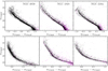 |
Fig. 1 CMDs of the studied clusters, namely NGC 1850, NGC 1818, and NGC 2164. The stars in the cluster field are represented with black dots, whereas the violet dots refer to the reference-field stars. For NGC 1850 we used stellar proper motions to identify and exclude from the analysis the bulk of field stars. |
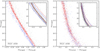 |
Fig. 2 mF336W vs. mF336W − mF814W (left) and mF336W vs. mF275W − mF336W (right) CMDs of stars in the NGC 1850 cluster field. The CMDs are zoomed-in around the luminosity interval that we used to investigate the incidence of binaries among the stellar populations with different rotation rates. The probable rMS and bMS stars, selected in the left-panel CMD, are colored red and blue, respectively, whereas the remaining stars are represented with gray dots. The insets show the fiducial lines of the rMS and bMS (continuous lines), and the fiducial lines of equal-luminosity bMS and rMS binaries (dashed lines). |
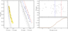 |
Fig. 3 mF336W vs. mF275W − mF336W (left panel), mF336W vs. mF336W − mF814W CMDs (middle panel), the verticalized mF336W vs. ΔF336W,F814W diagram (top-right panel), and the ΔF336W,F814W cumulative distributions (bottom-right panel). The investigated binaries, selected in the left CMD and located within the shadow yellow region, are colored black, whereas the remaining stars are represented with gray dots. The gray crosses in the top-right panel are stars excluded from the analysis. The red and blue lines are the fiducial lines for equal-luminosity rMS and bMS binaries, respectively. |
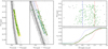 |
Fig. 4 Simulated mF336W vs. mF275W − mF336W (left) and mF336W vs. mF336W − mF814W CMDs (middle) of NGC 1850 that better reproduce the ΔF336W,F814W cumulative distribution of the observed binaries. The verticalized mF336W vs. ΔF336W,F814W diagram is plotted on the top-right panel. The probable binaries, selected from the left-panel CMD, are colored green. Like in Fig. 3, the orange lines in the left-panel CMD mark the boundaries of the yellow area, whereas the fiducial lines of the equal-luminosity bMS and rMS binaries are indicated with continuous blue and red lines, respectively. The bottom-right panel compares the ΔF336W,F814W cumulative distribution of the observed binaries (brown line) with the corresponding distribution for the simulated binaries. For completeness, we use the dashed blue and red lines to show the cumulative distributions derived from the simulated CMDs that host only bMS and rMS binaries, respectively. |
Fractions of bMS and rMS stars among the overall binary population.
3.2 The fractions of red-MS and blue-MS stars
To infer the fraction of rMS, bMS stars, and the fraction of binaries in the cluster field, we adopted the method described by Milone et al. (2012b). We defined three regions in the CMD, namely A, B, and C (see Fig. 6).
Regions A and B are mostly populated by bMS stars and rMS stars with 19.4 < mF336W < 20.75 mag, respectively. The limits of region A have been traced arbitrarily with the criteria of including most of the bMS stars. The red boundary of region B was evaluated starting from the rMS fiducial line and corresponds to the sequence of binaries with a mass ratio equal to 0.4. Region C includes binary systems with a mass ratio larger than 0.4. The red boundary of region C corresponds to the sequence of equal-mass rMS binaries shifted to red by the color error.
Due to observational errors, each region is affected by contamination of stars from the other populations. Therefore, the total number of stars, Ni that we observe in each region can be indicated as
![$\[N_{\mathrm{i}=\mathrm{A}, \mathrm{B}, \mathrm{C}}=N_{\mathrm{bMS}} f_{\mathrm{bMS}, \mathrm{i}}+N_{\mathrm{rMS}} f_{\mathrm{rMS}, \mathrm{i}}+N_{\mathrm{bin}} f_{\mathrm{bin}, \mathrm{i}}.\]$](/articles/aa/full_html/2024/12/aa51310-24/aa51310-24-eq3.png) (3)
(3)
Here, fbMS,i, frMS,i, and fbin,i are the fractions of bMS stars, rMS stars, and binaries in each region. These quantities are obtained from simulated CMDs composed of bMS, rMS, and binaries only, and derived by using ASs. The simulated binaries comprise the same fractions of bMS and rMS binaries that we inferred from the observations.
The quantities NbMS, NrMS, and Nbin represent the total numbers of bMS stars, rMS stars, and binary systems, respectively. To derive these values, we iteratively solved the system of linear equations (Eq. (3)). At the first iteration, we assumed that the cluster hosts no binaries, whereas in the subsequent iterations, we adopted NbMS, NrMS, and Nbin as guesses to improve these values. Since the fractions of binaries in the regions A, B, and C of the CMD depend on the numbers of bMS and rMS stars, at each iteration we derived an improved determination of the quantity fbin,i. We iterated the procedure until the values of NbMS, NrMS, and Nbin obtained in two subsequent iterations differ by less than 0.001. The fractions of bMS and rMS stars and the fraction of binaries are listed in Table 3 and confirm previous findings that the majority of MS stars belong to the rMS.
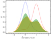 |
Fig. 5 Comparison between the observed ΔF336W,F814W kernel distribution of the NGC 1850 binaries (yellow-shaded area) and the corresponding distribution derived from the best-fitting simulated CMD (green-shaded area). The dashed blue and red lines indicate the distributions of binaries in a simulated CMD that hosts only bMS and rMS binaries, respectively. |
Fractions of bMS stars, rMS stars, and binaries in the studied clusters.
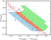 |
Fig. 6 mF336W vs. mF336W − mF814W CMD of the cluster field of NGC 1850. Blue, red, and green zones are delineated to encompass the majority of bMS, rMS, and binary stars, respectively. |
3.3 The fraction of binaries among blue-MS and red-MS stars
To derive the fractions of binaries among bMS and rMS stars, ![$\[F_{b M S}^{b i n}\]$](/articles/aa/full_html/2024/12/aa51310-24/aa51310-24-eq7.png) and
and ![$\[F_{r M S}^{b i n}\]$](/articles/aa/full_html/2024/12/aa51310-24/aa51310-24-eq8.png) , we combined the results from Sects. 3.1 and 3.2. Specifically, we used the relation
, we combined the results from Sects. 3.1 and 3.2. Specifically, we used the relation
![$\[\begin{aligned}F_{b M S}^{b i n} & =\frac{f_{b M S, b i n} \cdot N_{b i n}}{f_{b M S, b i n} \cdot N_{b i n}+N_{b M S}} \\F_{r M S}^{b i n} & =\frac{f_{r M S, b i n} \cdot N_{b i n}}{f_{r M S, b i n} \cdot N_{b i n}+N_{r M S}}.\end{aligned}\]$](/articles/aa/full_html/2024/12/aa51310-24/aa51310-24-eq9.png) (4)
(4)
For NGC 1850, we obtain fractions of binaries among the bMS and rMS stars of 23 ± 4% and 5 ± 4%, respectively. The results, presented in Table 3 and illustrated in Fig. 7, reveal a predominance of bMS binaries in all clusters. Specifically, the ratio between ![$\[F_{b M S}^{b i n}\]$](/articles/aa/full_html/2024/12/aa51310-24/aa51310-24-eq10.png) and
and ![$\[F_{r M S}^{b i n}\]$](/articles/aa/full_html/2024/12/aa51310-24/aa51310-24-eq11.png) ranges from ~4.60 ± 0.15 in NGC 1850 to ~1.50 ± 0.04 and ~1.90 ± 0.05 for NGC 1818 and NGC 2164, respectively.
ranges from ~4.60 ± 0.15 in NGC 1850 to ~1.50 ± 0.04 and ~1.90 ± 0.05 for NGC 1818 and NGC 2164, respectively.
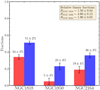 |
Fig. 7 Comparison between the fraction of binaries in bMS and rMS stars (blue and red bars, respectively) in the studied clusters. The inset indicates the fraction of bMS stars relative to the rMS binary fraction, |
![$\[F_{b M S}^{b i n} / F_{r M S}^{b i n}\]$](/articles/aa/full_html/2024/12/aa51310-24/aa51310-24-eq12.png)
4 Summary and conclusions
It is now widely accepted that star clusters younger than ~600 Myr exhibit split MSs. The rMSs, which include the majority of MS stars, are populated by fast-rotating stars, while the bMSs consist of slow-rotating stars (e.g., Milone & Marino 2022; Li et al. 2024, and references therein). Despite this, the origin of stars with varying rotation rates remains poorly understood. The main mechanisms proposed to explain the split MS include interactions in binary systems, the evolution of pre-MS stars, and stellar mergers. In this context, binary systems composed of bMS and rMS stars may provide insights that we can use to disentangle the different formation scenarios. Each scenario predicts different patterns of binarity between the two MSs. Specifically, a predominance of binaries among bMS stars would support the possibility that interactions in binary star systems are responsible for stellar braking (D’Antona et al. 2015, 2017), whereas if the split MS is due to the early evolution of pre-MS stars, we would expect similar fractions of bMS and rMS binaries (Bastian et al. 2020; Kamann et al. 2021). In contrast, in the scenario proposed by Wang et al. (2022), where the merging of binary systems is responsible for the origin of bMS stars, we would expect a predominance of binaries among rMS stars.
In this work, we present the first photometric derivation of the frequency of binaries in the bMS and rMSs of three young LMC clusters, namely NGC 1818, NGC 1850, and NGC 2164. To do this, we used high-precision photometry in the F814W, F336W, and F225W (or F275W) bands of UVIS/WFC3 of the HST (Milone et al. 2023a), refining the approach initially developed by Milone et al. (2020) for investigating binary stars among multiple populations in Galactic GCs.
In a nutshell, we utilized the mF336W versus mF225W − mF336W (or mF275W − mF336W) CMDs, in which the two MSs nearly overlap, to identify a sample of binaries composed of stars with similar luminosities. We then analyzed these binaries in the mF336W versus mF336W − mF814W CMDs, which maximize the color separation between bMS and rMS stars. We estimated the fractions of binaries among bMS and rMS stars by comparing the mF336W − mF814W color distribution of the observed binaries with grids of simulated CMDs that account for various binary fractions among bMS and rMS stars.
We observe a predominance of binaries among the bMS stars in all the studied clusters. The fractions of bMS binaries exceed those of rMS binaries by a factor of ~1.5 in NGC 1818, 4.6 in NGC 1850, and 1.9 in NGC 2164. Noticeably, these results are qualitatively similar to what is observed in the Galactic field, where binaries with periods between 4 and 500 days rotate much more slowly than single stars (Abt & Boonyarak 2004).
To understand the origin of the split MS in young Magellanic Cloud star clusters, D’Antona et al. (2015, 2017) propose that all cluster stars are born as fast rotators. Interactions in binary systems may be responsible for stellar braking, with tidal interactions causing braking effects that begin in the core and extend outward. When this braking process affects the stellar envelope and photosphere, the stars reach their final position on the bMS. Our finding of a predominance of binaries among the bMS stars aligns with the idea proposed by D’Antona and colleagues and suggests that their scenario represents the primary pathway for the formation of bMS stars.
Recently, Kamann et al. (2021) exploited multi-epoch observations of NGC 1850 collected with the integral field spectrograph MUSE at the Very Large Telescope to investigate the role of binarity in the origin of the split MS (see also Saracino et al. 2023). They conclude that the slowly and rapidly rotating populations host similar fractions of binaries, ~5%; this finding is in tension with the outcomes of our photometric study on NGC 1850 and with the results from Abt & Boonyarak (2004) for the Galactic field.
However, we observe that Kamann and collaborators’ spectroscopic analysis primarily detects hard binaries. In contrast, our study’s sample of photometric binaries encompasses all binaries with large mass ratios, regardless of their periods and semimajor axes. One possible way to reconcile the results of Kamann et al. (2021) with our findings is by considering that the soft binaries mostly populate the bMS of NGC 1850. In this scenario, the formation of bMS stars could be linked to tidal interactions within soft binaries, as proposed by He et al. (2023) and Yang et al. (2021).
Finally, we notice that the observed predominance of binaries may challenge the possibility that stellar mergers of MS stars are the main mechanisms responsible for the formation of bMS stars (Wang et al. 2022). In this case, we would expect a lack of binaries in the bMS. However, the lack of a quantitative analysis on the role of triple stellar systems in the merging process prevents us from drawing any firm conclusions.
Acknowledgements
We thank the anonymous referee for various suggestions that improved the quality of the manuscript. This work has been funded by the European Union — NextGenerationEU RRF M4C2 1.1 (PRIN 2022 2022MMEB9W: “Understanding the formation of globular clusters with their multiple stellar generations”, CUP C53D23001200006), from INAF Research GTO-Grant Normal RSN2-1.05.12.05.10 – (ref. Anna F. Marino) of the “Bando INAF per il Finanziamento della Ricerca Fondamentale 2022”, and from the European Union’s Horizon 2020 research and innovation programme under the Marie Skłodowska-Curie Grant Agreement No. 101034319 and from the European Union -– NextGenerationEU (beneficiary: T. Ziliotto). We thank the anonymous referee.
References
- Abt, H. A., & Boonyarak, C. 2004, ApJ, 616, 562 [NASA ADS] [CrossRef] [Google Scholar]
- Anderson, J., & King, I. R. 2000, PASP, 112, 1360 [NASA ADS] [CrossRef] [Google Scholar]
- Anderson, J., Sarajedini, A., Bedin, L. R., et al. 2008, AJ, 135, 2055 [Google Scholar]
- Bastian, N., & de Mink, S. E. 2009, MNRAS, 398, L11 [NASA ADS] [CrossRef] [Google Scholar]
- Bastian, N., Kamann, S., Cabrera-Ziri, I., et al. 2018, MNRAS, 480, 3739 [NASA ADS] [CrossRef] [Google Scholar]
- Bastian, N., Kamann, S., Amard, L., et al. 2020, MNRAS, 495, 1978 [NASA ADS] [CrossRef] [Google Scholar]
- Bertelli, G., Nasi, E., Girardi, L., et al. 2003, AJ, 125, 770 [NASA ADS] [CrossRef] [Google Scholar]
- Cordoni, G., Milone, A. P., Marino, A. F., et al. 2018, ApJ, 869, 139 [CrossRef] [Google Scholar]
- Cordoni, G., Milone, A. P., Marino, A. F., et al. 2022, Nat. Commun., 13, 4325 [NASA ADS] [CrossRef] [Google Scholar]
- Cordoni, G., Casagrande, L., Yu, J., et al. 2024, MNRAS, 532, 1547 [CrossRef] [Google Scholar]
- Correnti, M., Goudfrooij, P., Kalirai, J. S., et al. 2014, ApJ, 793, 121 [NASA ADS] [CrossRef] [Google Scholar]
- Cristofari, P. I., Dupree, A. K., Milone, A. P., et al. 2024, ApJ, 972, 72 [NASA ADS] [CrossRef] [Google Scholar]
- D’Antona, F., Di Criscienzo, M., Decressin, T., et al. 2015, MNRAS, 453, 2637 [NASA ADS] [Google Scholar]
- D’Antona, F., Milone, A. P., Tailo, M., et al. 2017, Nat. Astron., 1, 0186 [CrossRef] [Google Scholar]
- D’Antona, F., Dell’Agli, F., Tailo, M., et al. 2023, MNRAS, 521, 4462 [CrossRef] [Google Scholar]
- Dufton, P. L., Langer, N., Dunstall, P. R., et al. 2013, A&A, 550, A109 [NASA ADS] [CrossRef] [EDP Sciences] [Google Scholar]
- Dupree, A. K., Dotter, A., Johnson, C. I., et al. 2017, ApJ, 846, L1 [NASA ADS] [CrossRef] [Google Scholar]
- Georgy, C., Charbonnel, C., Amard, L., et al. 2019, A&A, 622, A66 [NASA ADS] [CrossRef] [EDP Sciences] [Google Scholar]
- Glatt, K., Grebel, E. K., Sabbi, E., et al. 2008, AJ, 136, 1703 [Google Scholar]
- Goudfrooij, P., Puzia, T. H., Kozhurina-Platais, V., & Chandar, R. 2011, ApJ, 737, 3 [NASA ADS] [CrossRef] [Google Scholar]
- Goudfrooij, P., Girardi, L., & Correnti, M. 2017, ApJ, 846, 22 [CrossRef] [Google Scholar]
- He, C., Li, C., Sun, W., et al. 2023, MNRAS, 525, 5880 [CrossRef] [Google Scholar]
- Kamann, S., Bastian, N., Usher, C., Cabrera-Ziri, I., & Saracino, S. 2021, MNRAS, 508, 2302 [NASA ADS] [CrossRef] [Google Scholar]
- Legnardi, M. V., Milone, A. P., Cordoni, G., et al. 2023, MNRAS, 522, 367 [CrossRef] [Google Scholar]
- Li, C., de Grijs, R., Deng, L., & Milone, A. P. 2017, ApJ, 844, 119 [CrossRef] [Google Scholar]
- Li, C., Milone, A. P., Sun, W., & de Grijs, R. 2024, arXiv e-prints [arXiv:2401.08062] [Google Scholar]
- Mackey, A. D., & Broby Nielsen, P. 2007, MNRAS, 379, 151 [NASA ADS] [CrossRef] [Google Scholar]
- Milone, A. P., & Marino, A. F. 2022, Universe, 8, 359 [NASA ADS] [CrossRef] [Google Scholar]
- Marino, A. F., Milone, A. P., Casagrande, L., et al. 2018a, ApJ, 863, L33 [NASA ADS] [CrossRef] [Google Scholar]
- Marino, A. F., Przybilla, N., Milone, A. P., et al. 2018b, AJ, 156, 116 [NASA ADS] [CrossRef] [Google Scholar]
- Milone, A. P., Bedin, L. R., Piotto, G., & Anderson, J. 2009, A&A, 497, 755 [NASA ADS] [CrossRef] [EDP Sciences] [Google Scholar]
- Milone, A. P., Piotto, G., Bedin, L. R., et al. 2012a, A&A, 540, A16 [NASA ADS] [CrossRef] [EDP Sciences] [Google Scholar]
- Milone, A. P., Piotto, G., Bedin, L. R., et al. 2012b, A&A, 537, A77 [NASA ADS] [CrossRef] [EDP Sciences] [Google Scholar]
- Milone, A. P., Bedin, L. R., Piotto, G., et al. 2015, MNRAS, 450, 3750 [CrossRef] [Google Scholar]
- Milone, A. P., Marino, A. F., D’Antona, F., et al. 2016, MNRAS, 458, 4368 [NASA ADS] [CrossRef] [Google Scholar]
- Milone, A. P., Marino, A. F., D’Antona, F., et al. 2017, MNRAS, 465, 4363 [NASA ADS] [CrossRef] [Google Scholar]
- Milone, A. P., Marino, A. F., Di Criscienzo, M., et al. 2018, MNRAS, 477, 2640 [Google Scholar]
- Milone, A. P., Vesperini, E., Marino, A. F., et al. 2020, MNRAS, 492, 5457 [Google Scholar]
- Milone, A. P., Cordoni, G., Marino, A. F., et al. 2023a, A&A, 672, A161 [NASA ADS] [CrossRef] [EDP Sciences] [Google Scholar]
- Milone, A. P., Cordoni, G., Marino, A. F., et al. 2023b, MNRAS, 524, 6149 [NASA ADS] [CrossRef] [Google Scholar]
- Mohandasan, A., Milone, A. P., Cordoni, G., et al. 2024, A&A, 681, A42 [NASA ADS] [CrossRef] [EDP Sciences] [Google Scholar]
- Niederhofer, F., Georgy, C., Bastian, N., & Ekström, S. 2015, MNRAS, 453, 2070 [NASA ADS] [CrossRef] [Google Scholar]
- Saracino, S., Kamann, S., Bastian, N., et al. 2023, MNRAS, 526, 299 [NASA ADS] [CrossRef] [Google Scholar]
- Wang, C., Langer, N., Schootemeijer, A., et al. 2022, Nat. Astron., 6, 480 [NASA ADS] [CrossRef] [Google Scholar]
- Yang, Y., Li, C., de Grijs, R., & Deng, L. 2021, ApJ, 912, 27 [NASA ADS] [CrossRef] [Google Scholar]
- Zahn, J. P. 1975, A&A, 41, 329 [NASA ADS] [Google Scholar]
- Zahn, J. P. 1977, A&A, 57, 383 [Google Scholar]
- Zorec, J., & Royer, F. 2012, A&A, 537, A120 [NASA ADS] [CrossRef] [EDP Sciences] [Google Scholar]
All Tables
Radii of the cluster field and minimum and maximum radii for the reference fields.
All Figures
|
Fig. 1 CMDs of the studied clusters, namely NGC 1850, NGC 1818, and NGC 2164. The stars in the cluster field are represented with black dots, whereas the violet dots refer to the reference-field stars. For NGC 1850 we used stellar proper motions to identify and exclude from the analysis the bulk of field stars. |
| In the text | |
|
Fig. 2 mF336W vs. mF336W − mF814W (left) and mF336W vs. mF275W − mF336W (right) CMDs of stars in the NGC 1850 cluster field. The CMDs are zoomed-in around the luminosity interval that we used to investigate the incidence of binaries among the stellar populations with different rotation rates. The probable rMS and bMS stars, selected in the left-panel CMD, are colored red and blue, respectively, whereas the remaining stars are represented with gray dots. The insets show the fiducial lines of the rMS and bMS (continuous lines), and the fiducial lines of equal-luminosity bMS and rMS binaries (dashed lines). |
| In the text | |
|
Fig. 3 mF336W vs. mF275W − mF336W (left panel), mF336W vs. mF336W − mF814W CMDs (middle panel), the verticalized mF336W vs. ΔF336W,F814W diagram (top-right panel), and the ΔF336W,F814W cumulative distributions (bottom-right panel). The investigated binaries, selected in the left CMD and located within the shadow yellow region, are colored black, whereas the remaining stars are represented with gray dots. The gray crosses in the top-right panel are stars excluded from the analysis. The red and blue lines are the fiducial lines for equal-luminosity rMS and bMS binaries, respectively. |
| In the text | |
|
Fig. 4 Simulated mF336W vs. mF275W − mF336W (left) and mF336W vs. mF336W − mF814W CMDs (middle) of NGC 1850 that better reproduce the ΔF336W,F814W cumulative distribution of the observed binaries. The verticalized mF336W vs. ΔF336W,F814W diagram is plotted on the top-right panel. The probable binaries, selected from the left-panel CMD, are colored green. Like in Fig. 3, the orange lines in the left-panel CMD mark the boundaries of the yellow area, whereas the fiducial lines of the equal-luminosity bMS and rMS binaries are indicated with continuous blue and red lines, respectively. The bottom-right panel compares the ΔF336W,F814W cumulative distribution of the observed binaries (brown line) with the corresponding distribution for the simulated binaries. For completeness, we use the dashed blue and red lines to show the cumulative distributions derived from the simulated CMDs that host only bMS and rMS binaries, respectively. |
| In the text | |
|
Fig. 5 Comparison between the observed ΔF336W,F814W kernel distribution of the NGC 1850 binaries (yellow-shaded area) and the corresponding distribution derived from the best-fitting simulated CMD (green-shaded area). The dashed blue and red lines indicate the distributions of binaries in a simulated CMD that hosts only bMS and rMS binaries, respectively. |
| In the text | |
|
Fig. 6 mF336W vs. mF336W − mF814W CMD of the cluster field of NGC 1850. Blue, red, and green zones are delineated to encompass the majority of bMS, rMS, and binary stars, respectively. |
| In the text | |
|
Fig. 7 Comparison between the fraction of binaries in bMS and rMS stars (blue and red bars, respectively) in the studied clusters. The inset indicates the fraction of bMS stars relative to the rMS binary fraction, |
| In the text | |
Current usage metrics show cumulative count of Article Views (full-text article views including HTML views, PDF and ePub downloads, according to the available data) and Abstracts Views on Vision4Press platform.
Data correspond to usage on the plateform after 2015. The current usage metrics is available 48-96 hours after online publication and is updated daily on week days.
Initial download of the metrics may take a while.