| Issue |
A&A
Volume 697, May 2025
|
|
|---|---|---|
| Article Number | A126 | |
| Number of page(s) | 19 | |
| Section | Planets, planetary systems, and small bodies | |
| DOI | https://doi.org/10.1051/0004-6361/202453434 | |
| Published online | 21 May 2025 | |
Gravito-turbulent bi-fluid protoplanetary discs
I. An analytical perspective to stratification
1
Leibniz-Institut für Astrophysik Potsdam (AIP),
Potsdam,
Germany
2
Università degli Studi di Milano, Dipartimento di Fisica,
via Celoria 16,
20133
Milano,
Italy
★ Corresponding author: srendon@aip.de
Received:
13
December
2024
Accepted:
17
March
2025
Context. In Class 0 and I as well as in the outskirts of Class II circumstellar discs, the self-gravity of gas is expected to be significant, which certainly impacts the disc vertical hydrostatic equilibrium. Notably, the contribution of dust, whose measured mass is still uncertain, could also be a factor in this equilibrium.
Aims. We aim to formulate and solve, approximately, the equations governing the hydrostatic equilibrium of a self-gravitating disc composed of gas and dust. Particularly, we aim to provide a fully consistent treatment of turbulence and gravity that almost symmetrically affects gas and dust. From an observational perspective, we study the possibility of indirectly measuring disc masses through gas layering and dust settling measurements.
Methods. We used analytical methods to approximate the solution of the 1D Liouville equation with additional non-linearities governing the stratification of a self-gravitating protoplanetary disc. The analytical findings were verified through numerical treatment, and their consistency was validated with a physical interpretation.
Results. For a constant vertical stopping time profile, we discovered a nearly exact layering solution valid across all self-gravity regimes for gas and dust. From first principles, we defined the Toomre parameter of a bi-fluid system as the harmonic average of its constituents’ Toomre parameters. Based on these findings, we propose a method to estimate disc mass through gas or dust settling observations. We introduce a generic definition of the dust-to-gas scale height that is applicable to complex profiles. Additionally, we identified new exact solutions useful for benchmarking self-gravity solvers in numerical codes.
Conclusions. The hydrostatic equilibrium of a gas-dust mixture is governed by their Toomre parameters and their effective relative temperature. The equilibrium we found could possibly be used for measuring disc masses, thus enabling a more thorough understanding of disc settling and gravitational collapse, and it will also improve the computation of self-gravity in thin disc simulations.
Key words: accretion, accretion disks / gravitation / turbulence / protoplanetary disks
© The Authors 2025
 Open Access article, published by EDP Sciences, under the terms of the Creative Commons Attribution License (https://creativecommons.org/licenses/by/4.0), which permits unrestricted use, distribution, and reproduction in any medium, provided the original work is properly cited.
This article is published in open access under the Subscribe to Open model. Subscribe to A&A to support open access publication.
1 Introduction
Protoplanetary accretion discs (PPDs) get their name from the process of material infalling into their host star. This accretion mechanism is associated with the outward transport of angular momentum, a process thought to originate from magnetised disc winds or a possible source of turbulence. The latter process can be driven by one of the main families of instabilities: magnetohydrodynamical instabilities (Balbus & Hawley 1991) or thermo-hydrodynamical instabilities, which includes the vertical shear instability, convective overstability, and zombie vortex instability (Nelson et al. 2013; Klahr & Hubbard 2014; Barranco & Marcus 2005; Marcus et al. 2013). We can also include resonant drag instabilities (Squire & Hopkins 2018), which arise from aerodynamic interactions between gas and dust. A particular case of these instabilities is the notable streaming instability (Youdin & Goodman 2005; Johansen & Youdin 2007). Finally, young discs or the outer regions of Class I and II discs are subject to the gravitational instability (GI; Gammie 2001; Kratter & Lodato 2016).
Measuring accretion rates, which range from 10−10 to 10−7 M⊙/yr (Venuti et al. 2014; Hartmann et al. 2016; Manara et al. 2016), is one of the possible ways to estimate the intensity of turbulence (Hartmann et al. 1998). Turbulence strength in PPDs can also be determined through Doppler broadening of spectral data, molecular emission of CO lines (Carr et al. 2004; Flaherty et al. 2020), and observation of the settling of dust particles in the disc midplane. Indeed, particle settling, promoted by a star’s gravity, is balanced by ascending turbulent transport, which allows one to relate the dust-to-gas scale height ratio to the vertical diffusion and Stokes number (Dubrulle et al. 1995). From millimetre observations, most Class II discs exhibit a significant level of dust settling in their outer discs (e.g. HL Tau, Oph 163131, and HD 163296 (Pinte et al. 2016; Villenave et al. 2020, 2022; Doi & Kataoka 2021; Pizzati et al. 2023)), thus indicating very low levels of turbulence. Therefore, it seems evident that the incorporation of additional relevant effects to the vertical hydrostatic equilibrium of the disc will allow for finer gas and dust stratifications and possibly permit access to more properties of the disc. One of these additional ingredients could be the effect of the disc’s gravity on itself, colloquially known as self-gravity (SG).
When the disc SG is insignificant compared to the star’s gravity, the gas and dust adopt a Gaussian vertical profile (Armitage 2019, Eqs. (15) and (238)). This is a situation that is assumed for measuring the dust-to-gas scale height ratio in Class I and II discs (Miotello et al. 2023, see Sect. 2.3.1). Conversely, in Class 0 and I discs, the disc SG dominates. This is typically seen in systems where mass infall is still ongoing, such as the Elias 2-27 system (Pérez et al. 2016; Veronesi et al. 2021), or in the cold outer regions of PPDs, as in the RU Lup system (Huang et al. 2020). For such a case, it was found that the gas vertical density stratification obeys a hyperbolic secant profile corresponding to the limit of a small Toomre parameter (Spitzer 1942; Bertin & Lodato 1999). The same profile was also obtained in a dust rich environment by Klahr & Schreiber (2020, 2021), where they also defined a dust Toomre parameter. The aforementioned profiles, however, consider independent contributions of gas and dust SG to their own respective stratification. In other words, from a gravitational point of view, gas interacts solely with gas and dust interacts solely with dust, a scenario that might hold true in certain instances but is not generally applicable. A more sophisticated model involves taking into account the star’s gravity and the disc SG by using a biased Gaussian stratification, where all SG information is incorporated into a modified scale height, which is naturally dependent on Toomre parameter (Bertin & Lodato 1999). This improvement allows for a smooth transition between Keplerian discs and massive discs. The most comprehensive model to date, developed by Baehr & Zhu (2021), attempted to capture the effect of the star’s gravity and the disentangled SG of gas and dust into the solid material.
It is worth noting that existing analytic models of disc layering that account for dust stirring in a turbulent gas environment often disregard the effect of turbulence on the gas itself. In reality, turbulence should act as a pressure term for the gas (Bonazzola et al. 1986). Therefore, to ensure consistency with the assumption of dust embedded in a turbulent gaseous environment, it is important to also assume that the gas itself is subject to turbulence. This could permit improvement of the models of Dubrulle et al. (1995), Takeuchi & Lin (2002), Fromang & Nelson (2009), and Klahr & Schreiber (2021), where gas is considered a passive tracer that keeps its Gaussian stratification and scale height, which is not necessarily true in the presence of turbulence and even less so when there is SG. This has been confirmed by the study of Baehr & Zhu (2021), where thanks to 3D shearing box simulations, they were able to show that the consideration of gas and dust SG on particles has significant consequences on the gas and dust settling. Thus, more sophisticated models are needed to capture the turbulence and SG affecting both gas and dust.
In a different context (which was the initial focus of this work), accurately estimating gas and dust scale heights was found to significantly impact the calculation of SG forces in thin disc (2D) simulations. These simulations typically use a Plummer potential with a smoothing length for gravity prescription (Müller et al. 2012). Rendon Restrepo & Barge (2023) demonstrated that while this method correctly models long-range SG interactions, it underestimates mid- and short-range interactions by up to 100%, aligning with the removal of Newtonian behaviour due to softening (Adams et al. 1989; Hockney & Eastwood 2021). Conversely, without smoothing, SG is highly overestimated. To address this, a space-varying smoothing length was introduced to better match the 2D SG force with its 3D counterpart. Further, Rendon Restrepo & Barge (2023) extended their correction to bi-fluids with an embedded dust phase, finding that two additional smoothing lengths are needed to account for dust-dust and dust-gas gravitational interactions. Their afore-mentioned length depends heavily on the scale heights of gas and dust, making the vertical layering of a PPD crucial for accurate SG computation in 2D simulations. This is particularly important for massive discs, where consistency between vertical layering and in-plane SG computation is required.
In this first article, of a series of two, we study the stratification of gas and dust in the presence of turbulence and their disentangled SG contributions by analytical means. In the second paper, using 3D hydrodynamical shearing box simulations, we study how these results could potentially affect planetesimal formation and gas accretion. We begin by detailing our assumptions and establishing the equations of hydrostatic equilibrium for gas and dust in Sect. 2. In Sects. 3–4 we propose, depending on the assumption made on the vertical profile of the stopping time, different exact or general approximated solutions valid for any gravity contribution strength (i.e. from the star, gas, or dust). In Sect. 5, we show how our results could permit indirect access to the mass content of a PPD. Finally, in Sect. 6, we propose a discussion on the limitations of our approach, the possible consequences for planetesimal formation, and the consequences for SG computation in thin disc simulations. Important equations and detailed derivations can be found in the appendices.
2 Formulating the main equations
In this section, we derive the two main equations describing the vertical hydrostatic equilibrium of gas and steady-state transport of dust in the presence of turbulence and SG. However, we first introduce our notation conventions.
2.1 Guidelines and cautions
We account for turbulence as an additional pressure term in the gas and a diffusion term for dust. Both give rise to effective sound speeds, which we denote by a tilde: ( ˜ ). For example, ![\[{\tilde c_g}\]](/articles/aa/full_html/2025/05/aa53434-24/aa53434-24-eq1.png) stands for the modified gas sound speed accounting for turbulence. The vertical stratification of a self-gravitating disc is a challenging problem that requires a redefinition of several physical quantities. For instance, intuitively, we expect the vertical scale heights to be reduced, which could be interpreted as a greater differential rotation in the midplane. Therefore, the differential rotation in the presence of SG is also modified, which (surprisingly) changes the definition of the Toomre parameters as well. Therefore, in order to avoid confusion, we use a superscript ‘sg’ as soon as a quantity is redefined in the presence of SG. Furthermore, a subscript ‘g’ or ‘d’ is used to make a distinction between gas and dust quantities, respectively. If there is no special superscript, it means that we are using the reference notation used in the literature. All of these cautions are particularly important for Sects. 3 and 4. Finally, the “mid” subscript indicates that quantities are taken in the equatorial plane, z = 0. In Table 1, we collect the definition of all quantities used in this study.
stands for the modified gas sound speed accounting for turbulence. The vertical stratification of a self-gravitating disc is a challenging problem that requires a redefinition of several physical quantities. For instance, intuitively, we expect the vertical scale heights to be reduced, which could be interpreted as a greater differential rotation in the midplane. Therefore, the differential rotation in the presence of SG is also modified, which (surprisingly) changes the definition of the Toomre parameters as well. Therefore, in order to avoid confusion, we use a superscript ‘sg’ as soon as a quantity is redefined in the presence of SG. Furthermore, a subscript ‘g’ or ‘d’ is used to make a distinction between gas and dust quantities, respectively. If there is no special superscript, it means that we are using the reference notation used in the literature. All of these cautions are particularly important for Sects. 3 and 4. Finally, the “mid” subscript indicates that quantities are taken in the equatorial plane, z = 0. In Table 1, we collect the definition of all quantities used in this study.
Definitions.
2.2 Hydrostatic equilibrium of gas
We assumed that the gas is in a turbulent situation. Accordingly, we employed the Reynolds averaging method (Reynolds 1895; Krause & Rüdiger 1974) and decomposed all velocity components of gas as the sum of a mean and a fluctuating part: ![\[{v_i} = \overline {{v_i}} + {v_{i'}}\]](/articles/aa/full_html/2025/05/aa53434-24/aa53434-24-eq17.png) . The bar designates a time average. A proper treatment of turbulence would also require decomposing the pressure and density variables into a mean and fluctuating part and consideration of the compressibility of the flow. Using Favre averages is a more appropriate approach for this situation (Favre 1965, 1992), but it complicates the definition of diffusion terms and makes it challenging to compare our work with existing literature that uses Reynolds averaging. Consequently, in this work, we assume that pressure and density are equal to their statistical mean value. Despite this simplifying assumption, our model still represents an improvement over other models that ignore the effects of turbulence on the gas itself, such as those proposed by Fromang & Nelson (2009) and Baehr & Zhu (2021). By taking turbulence into account solely through velocity fluctuations, we keep the problem analytically tractable. Assuming hydrostatic equilibrium,
. The bar designates a time average. A proper treatment of turbulence would also require decomposing the pressure and density variables into a mean and fluctuating part and consideration of the compressibility of the flow. Using Favre averages is a more appropriate approach for this situation (Favre 1965, 1992), but it complicates the definition of diffusion terms and makes it challenging to compare our work with existing literature that uses Reynolds averaging. Consequently, in this work, we assume that pressure and density are equal to their statistical mean value. Despite this simplifying assumption, our model still represents an improvement over other models that ignore the effects of turbulence on the gas itself, such as those proposed by Fromang & Nelson (2009) and Baehr & Zhu (2021). By taking turbulence into account solely through velocity fluctuations, we keep the problem analytically tractable. Assuming hydrostatic equilibrium, ![\[\overline {{v_z}} = 0\]](/articles/aa/full_html/2025/05/aa53434-24/aa53434-24-eq18.png) , and that the density, pressure, and turbulent
, and that the density, pressure, and turbulent ![\[\overline {{v_{i'}}{v_{j'}}} \]](/articles/aa/full_html/2025/05/aa53434-24/aa53434-24-eq19.png) terms are only z-dependent, we obtained the Reynolds equation for the gas in the vertical direction:
terms are only z-dependent, we obtained the Reynolds equation for the gas in the vertical direction:
![\[\frac{1}{{{\rho _g}}}{\partial _z}\left( {p + \overline {{\rho _g}v_z^{_'}v_z^{_'}} } \right) = \overline {F_z^g} ,\]](/articles/aa/full_html/2025/05/aa53434-24/aa53434-24-eq20.png) (1)
where
(1)
where ![\[F_z^g\]](/articles/aa/full_html/2025/05/aa53434-24/aa53434-24-eq21.png) represents all volume forces applied to the gas, which is discussed in more detail in Sect. 2.4. The gas is assumed to be in a vertical isothermal state,
represents all volume forces applied to the gas, which is discussed in more detail in Sect. 2.4. The gas is assumed to be in a vertical isothermal state, ![\[p = c_g^2{\rho _g}\]](/articles/aa/full_html/2025/05/aa53434-24/aa53434-24-eq22.png) , where cg is the isothermal sound speed. The Reynolds stress term,
, where cg is the isothermal sound speed. The Reynolds stress term, ![\[\overline {{v_{z'}}{v_{z'}}} \]](/articles/aa/full_html/2025/05/aa53434-24/aa53434-24-eq23.png) , can be rewritten in terms of a diffusion term in the α-viscosity paradigm (Shakura & Sunyaev 1973):
, can be rewritten in terms of a diffusion term in the α-viscosity paradigm (Shakura & Sunyaev 1973):
![\[{\alpha _{\rm{z}}} = \frac{{\overline {{\rho _g}v_z^'v_z^'} }}{{\overline {c_g^2{\rho _g}} }}.\]](/articles/aa/full_html/2025/05/aa53434-24/aa53434-24-eq24.png) (2)
(2)
To simplify our approach, we assumed that the above expression for the turbulent diffusivity is constant with respect to z. This assumption, which in general is not true (Nelson et al. 2013; Flock et al. 2020; Baehr & Zhu 2021), allows the problem to be accessible analytically. It is important to note that in a majority of numerical and theoretical studies, the radial Reynolds stress, ![\[{\alpha _S} = \overline {{\rho _g}v_r^'v_\phi ^'} /\overline {c_g^2{\rho _g}} \]](/articles/aa/full_html/2025/05/aa53434-24/aa53434-24-eq25.png) , responsible for transporting angular momentum in the radial direction is frequently employed in place of the vertical stress. This stress is related to its vertical analogue through the equation αz = αS /Scz, where Scz is the vertical Schmidt number, which quantifies the level of anisotropy in turbulence. In the context of a PPD, the parameter αz can take different values depending on the region of the disc, its age, and most importantly on the type of instability generating the turbulence (Lesur et al. 2023). Introducing the effective gas sound speed,
, responsible for transporting angular momentum in the radial direction is frequently employed in place of the vertical stress. This stress is related to its vertical analogue through the equation αz = αS /Scz, where Scz is the vertical Schmidt number, which quantifies the level of anisotropy in turbulence. In the context of a PPD, the parameter αz can take different values depending on the region of the disc, its age, and most importantly on the type of instability generating the turbulence (Lesur et al. 2023). Introducing the effective gas sound speed, ![\[{\widetilde c_g} = \sqrt {1 + {\rm{ }}{\alpha _{\rm{z}}}} {\mkern 1mu} {c_g}\]](/articles/aa/full_html/2025/05/aa53434-24/aa53434-24-eq26.png) , the vertical hydrostatic equilibrium for gas can be rewritten as
, the vertical hydrostatic equilibrium for gas can be rewritten as
![\[\widetilde c_g^2{\partial _z}\ln \left( {{\rho _g}} \right) = \overline {F_z^g} .\]](/articles/aa/full_html/2025/05/aa53434-24/aa53434-24-eq27.png) (3)
(3)
2.3 Transport equation for dust
The dust stirring stems from aerodynamic coupling of small grains, ΩKτf < 1, with the turbulent gaseous environment, which allows one to make use of the transport equation for dust (Dubrulle et al. 1995; Schräpler & Henning 2004, Eq. (28)):
![\[{\partial _t}{\rho _d} + {\partial _z}\left[ {{\tau _f}{\rho _d}F_z^d - {\rho _g}{\kappa _t}{\partial _z}\left( {\frac{{{\rho _d}}}{{{\rho _g}}}} \right)} \right] = 0,\]](/articles/aa/full_html/2025/05/aa53434-24/aa53434-24-eq28.png) (4)
where
(4)
where ![\[F_z^d\]](/articles/aa/full_html/2025/05/aa53434-24/aa53434-24-eq29.png) are all volume forces applied to dust, except the aerodynamic force (see Sect. 2.4). The third term on the left-hand side represents the diffusion flux of solid material. The stop-ping time and turbulent diffusivity are depicted by τf and κt, respectively. Assuming dust to be in a steady state in the vertical direction, we obtain
are all volume forces applied to dust, except the aerodynamic force (see Sect. 2.4). The third term on the left-hand side represents the diffusion flux of solid material. The stop-ping time and turbulent diffusivity are depicted by τf and κt, respectively. Assuming dust to be in a steady state in the vertical direction, we obtain
![\[c_d^2{\partial _z}\ln \left( {\frac{{{\rho _d}}}{{{\rho _g}}}} \right) = F_z^d,\]](/articles/aa/full_html/2025/05/aa53434-24/aa53434-24-eq30.png) (5)
where
(5)
where ![\[{c_d} = \sqrt {{\kappa _t}/{\tau _f}} \]](/articles/aa/full_html/2025/05/aa53434-24/aa53434-24-eq31.png) can be interpreted as a dust sound speed. This stems from a direct analogy with the vertical hydrostatic equilibrium of gas (Eq. (3)). However, this comparison, although direct, remains rather empirical. Therefore, we have decided to summarise, adapt, and generalise the approach proposed by Klahr & Schreiber (2021, Appendix B) in the next paragraph, as it is more rigorous.
can be interpreted as a dust sound speed. This stems from a direct analogy with the vertical hydrostatic equilibrium of gas (Eq. (3)). However, this comparison, although direct, remains rather empirical. Therefore, we have decided to summarise, adapt, and generalise the approach proposed by Klahr & Schreiber (2021, Appendix B) in the next paragraph, as it is more rigorous.
First, we redefined the velocity of the solid material as ![\[\nu _d^* = {\nu _d} - {\kappa _t}\frac{{{\rho _g}}}{{{\rho _d}}}\nabla \left( {\frac{{{\rho _d}}}{{{\rho _g}}}} \right)\]](/articles/aa/full_html/2025/05/aa53434-24/aa53434-24-eq32.png) and proposed a new momentum equation associated with the evolution of this velocity field. The revised momentum equation resembles the momentum equation of dust but includes an unknown source term, 𝒮, which drives diffusion and must be determined. By employing the procedure of the previously mentioned authors, we obtained the expression of the source term as
and proposed a new momentum equation associated with the evolution of this velocity field. The revised momentum equation resembles the momentum equation of dust but includes an unknown source term, 𝒮, which drives diffusion and must be determined. By employing the procedure of the previously mentioned authors, we obtained the expression of the source term as
![\[{\cal S} = - \frac{{{\kappa _t}}}{{{\tau _f}}}{\partial _z}\ln \left( {\frac{{{\rho _d}}}{{{\rho _g}}}} \right).\]](/articles/aa/full_html/2025/05/aa53434-24/aa53434-24-eq33.png) (6)
(6)
This term acts as a vertical gradient of a pressure-like term for dust, allowing Eq. (5) to be interpreted as the hydrostatic equilibrium between the pressure of dust and the vertical forces promoting dust settling. The derived sound speed, cd, differs from the root mean square (rms) velocity of particles as discussed by Klahr & Schreiber (2021, Sect. 2). We highlight that our expression for 𝒮 differs from the one suggested by Klahr & Schreiber (2021, Eq. (B11)). Indeed, they assumed that ρg is a space constant, an assumption that we have relaxed to allow for greater generality.
2.4 The vertical hydrostatic equilibrium equations of a gas and dust self-gravitating turbulent disc
In this work, we consider the vertical equilibrium of a PPD made of gas and dust and orbiting around a central object. For the sake of simplicity, we neglect the effect of magnetic pressure, B2/8π. We assumed that both species are subject to the star’s gravity, the disc’s SG, and their mutual aerodynamic interaction. The body forces for gas and dust are given by
![\[\bar F_z^g = F_z^d = - \Omega _K^2z - {\partial _z}{\Phi _{disc}},\]](/articles/aa/full_html/2025/05/aa53434-24/aa53434-24-eq34.png) (7)
where ΩK stands for the Keplerian frequency and Φdisc is the gravitational potential of the disc made of gas and dust. In the limit of a flattened system, the vertical component of SG prevails over other components, and we can make use of Paczynski’s, or the slab, approximation (Spitzer 1942; Paczynski 1978; Binney & Tremaine 2008, Sect. 2.3.3):
(7)
where ΩK stands for the Keplerian frequency and Φdisc is the gravitational potential of the disc made of gas and dust. In the limit of a flattened system, the vertical component of SG prevails over other components, and we can make use of Paczynski’s, or the slab, approximation (Spitzer 1942; Paczynski 1978; Binney & Tremaine 2008, Sect. 2.3.3):
![\[\partial _{zz}^2{\Phi _{disc}} = 4\pi G\left( {{\rho _g} + {\rho _d}} \right).\]](/articles/aa/full_html/2025/05/aa53434-24/aa53434-24-eq35.png) (8)
(8)
We note that within this assumption, the variation of the potential at a given position is solely influenced by the mass distribution at that specific location, rather than the mass distribution throughout the entire disc. Putting together Eqs. (3), (5), (7), and (8), the stratifications of gas and dust are coupled via
![\[\left\{ {\begin{array}{*{20}{c}} {\tilde c_g^2{\partial _z}\ln \left( {{\rho _g}} \right)}&{ = - \Omega _K^2{\mkern 1mu} z - 2\pi G\left( {{\Sigma _g}(r,z) + {\Sigma _d}(r,z)} \right)}\\ {c_d^2{\partial _z}\ln \left( {{\rho _d}/{\rho _g}} \right)}&{ = - \Omega _K^2{\mkern 1mu} z - 2\pi G\left( {{\Sigma _g}(r,z) + {\Sigma _d}(r,z)} \right),} \end{array}} \right.\]](/articles/aa/full_html/2025/05/aa53434-24/aa53434-24-eq36.png) (9)
where
(9)
where ![\[{\Sigma _i}(r,z) = \int\limits_{ - z}^z {{\rho _i}} (r,z'){\mkern 1mu} dz'\]](/articles/aa/full_html/2025/05/aa53434-24/aa53434-24-eq37.png) is the vertically integrated density of gas and dust and r is the position vector in polar coordinates. The above equation expresses that gas, resp. dust, stratification is set by the balance between the star’s and the PPD’s SG and pressure, resp. turbulent vertical diffusion. The Eq. (9) requires additional constraints, which in the present case are obtained self-consistently thanks to the definition of the column densities:
is the vertically integrated density of gas and dust and r is the position vector in polar coordinates. The above equation expresses that gas, resp. dust, stratification is set by the balance between the star’s and the PPD’s SG and pressure, resp. turbulent vertical diffusion. The Eq. (9) requires additional constraints, which in the present case are obtained self-consistently thanks to the definition of the column densities:
![\[{\Sigma _i}(r) = {\Sigma _i}(r,z = \infty ) = \int_{ - \infty }^\infty {{\rho _i}} (r,z'){\mkern 1mu} dz'.\]](/articles/aa/full_html/2025/05/aa53434-24/aa53434-24-eq38.png) (10)
(10)
This closure condition is particularly interesting since the disc mass, and thus indirectly column densities, are the quantities that can be probed thanks to optically thin tracers, such as C 18O or N2H+ (Zhang et al. 2021; Trapman et al. 2022). Finally, the additional constraints lie in the assumptions made on the stopping time.
In the following sections, we initially address the broader scenario of a stopping time with a vertical profile. We then proceed to the simpler assumption of a constant stopping time.
3 Stopping time with vertical profile and negligible dust mass
We assumed that the turbulent diffusivity coefficient κt is constant but the stopping time has a density dependence:
![\[{\tau _f} = {\tau _{f,{\rm{mid}}}}\frac{{{\rho _{g,{\rm{mid}}}}}}{{{\rho _g}}}.\]](/articles/aa/full_html/2025/05/aa53434-24/aa53434-24-eq39.png) (11)
(11)
For instance, this realistic consideration means that small solid material, St = τf ΩK ≪ 1, is less coupled to gas in the upper layers of the disc. Further, we assume in this section that the dust mass is negligible compared to the gas mass. Using Eq. (11), it is convenient to reformulate the set of Eqs. (9) as a single equation for the unknown ρg and a transformation that permits one to retrieve ρd from ρg:
![\[\left\{ {\begin{array}{*{20}{l}} {\widetilde c_g^2\partial _{zz}^2\ln \left( {{\rho _g}} \right)}& = &{ - \Omega _K^2 - 4\pi G{\rho _g}}\\ {{\rho _d}}& = &{A(r){\mkern 1mu} {\rho _g}{\mkern 1mu} \exp \left( { - {\xi ^2}{\mkern 1mu} \frac{{{\rho _{g,{\rm{mid}}}}}}{{{\rho _g}}}} \right)} \end{array},} \right.\]](/articles/aa/full_html/2025/05/aa53434-24/aa53434-24-eq40.png) (12)
with
(12)
with ![\[\xi = {\widetilde c_g}/{c_{d,{\rm{mid}}}} = \sqrt {\frac{{(1 + \alpha )}}{{{\alpha _{\rm{z}}}}}{\rm{ St}}} \]](/articles/aa/full_html/2025/05/aa53434-24/aa53434-24-eq41.png) . The integration factor A(r) is to be fixed by the constraint in Eq. (10).
. The integration factor A(r) is to be fixed by the constraint in Eq. (10).
3.1 An exact solution for massive gas discs
In the case of a massive gas disc, that is, when ρd ≪ ρg and the gas Toomre parameter ![\[{Q_g} = \frac{{{{\widetilde c}_g}{\Omega _K}}}{{\pi G{\Sigma _g}}} \ll 1\]](/articles/aa/full_html/2025/05/aa53434-24/aa53434-24-eq42.png) , we found an exact solution to Eq. (12) given by
, we found an exact solution to Eq. (12) given by
![\[\left\{ {\begin{array}{*{20}{l}} {{\rho _g}(r,z)}& = &{\frac{{{\Sigma _g}}}{{2{Q_g}{H_g}}}{\rm{ sec}}{{\rm{h}}^2}\left( {\frac{z}{{{Q_g}{H_g}}}} \right)}\\ {{\rho _d}(r,z)}& = &{\frac{{{\Sigma _d}}}{{2{Q_g}\exp \left( {{\xi ^2}} \right){I_1}(\xi ){H_g}}}{\rm{ sec}}{{\rm{h}}^2}\left( {\frac{z}{{{Q_g}{H_g}}}} \right)}\\ {}&{}&{\quad \exp \left[ { - {\xi ^2}\left( {{{\cosh }^2}\left( {\frac{z}{{{Q_g}{H_g}}}} \right) - 1} \right)} \right]} \end{array},} \right.\]](/articles/aa/full_html/2025/05/aa53434-24/aa53434-24-eq43.png) (13)
where
(13)
where ![\[{H_g} = {\widetilde c_g}/{\Omega _K}\]](/articles/aa/full_html/2025/05/aa53434-24/aa53434-24-eq44.png) is the turbulent modified pressure scale height and
is the turbulent modified pressure scale height and
![\[{I_1}(\xi ) = \frac{{{\xi ^2}}}{2}\exp \left( { - \frac{{{\xi ^2}}}{2}} \right)\left[ {{K_1}\left( {\frac{{{\xi ^2}}}{2}} \right) - {K_0}\left( {\frac{{{\xi ^2}}}{2}} \right)} \right],\]](/articles/aa/full_html/2025/05/aa53434-24/aa53434-24-eq45.png) (14)
with Kν as a modified Bessel function of the second kind and of order ν. The detailed derivation of the integration constant A(r, φ) can be found in Appendix B.1. As expected, we retrieved the Spitzer solution for the gas layering (Spitzer 1942) and a more sophisticated profile for dust consisting of an envelope function (set by the gas vertical profile) and a function with rapid decline. To our knowledge, the solution for the dust profile is new. It is worth mentioning that Eq. (13) is the counterpart of Takeuchi & Lin (2002, Eq. (31)) and Fromang & Nelson (2009, Eq. (19)) that is valid for massive gas discs.
(14)
with Kν as a modified Bessel function of the second kind and of order ν. The detailed derivation of the integration constant A(r, φ) can be found in Appendix B.1. As expected, we retrieved the Spitzer solution for the gas layering (Spitzer 1942) and a more sophisticated profile for dust consisting of an envelope function (set by the gas vertical profile) and a function with rapid decline. To our knowledge, the solution for the dust profile is new. It is worth mentioning that Eq. (13) is the counterpart of Takeuchi & Lin (2002, Eq. (31)) and Fromang & Nelson (2009, Eq. (19)) that is valid for massive gas discs.
For completeness, we also decided to establish the domain of validity of the Spitzer model for gas. Accordingly, we depict in Fig. 1 the numeric solution of Eq. (12) and the Spitzer solution for different gas Toomre parameters ranging from 0.001 to 1. In this plot, we consider only the gas profile. We observed that for Qg ≳ 0.1, the Spitzer model no longer correctly describes the solution of the hydrostatic equilibrium of a self-gravitating gas disc. This encouraged us to clarify that a disc in a strong SG regime is a disc where the Toomre parameter lies below 0.1 and that a value of Qg ≃ 1 indicates a scenario where the gravitational contributions of the star and the gas disc are comparable, meaning neither is significantly greater than the other. Therefore, the Spitzer profile is valid only when Qg ≲ 0.1, and consequently, our solution including dust (Eq. (13)) is also valid under this condition.
It is important to note that the standard definition of Toomre parameter, as introduced by Toomre (1964), is derived from analysis of in-plane perturbations in an infinitely thin disc. This definition is given by Qg = κcg/(πGΣg), where the epicyclic frequency κ accounts for Keplerian rotation, the radial pressure gradient, and the radial component of the SG force. In contrast, our study disregards in-plane effects and focuses solely on vertical effects. Consequently, in our framework, the epicyclic frequency is simply equal to the Keplerian frequency, leading to the definition used in this work: Qg = ΩKcg/(πGΣg).
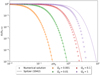 |
Fig. 1 Normalised gas density profile for various Toomre parameters (Qg) comparing the numerical solution of Eq. (12) with the Spitzer solution. |
3.2 An approximated solution for any gas disc mass
The previous model can be modified to include the force contribution of the star. Currently, the vertical stratification of a gaseous disc subject to both the vertical component of the star’s and its own gravity remains unsolved. However, we know of an approximate solution that made use of a biased Gaussian stratification assumption, incorporating all information about SG into a modified scale height (Bertin & Lodato 1999; Lodato 2007; Kratter & Lodato 2016). We refer to this approximate solution as the BL model. This model permits a smooth transition between a Keplerian and a self-gravitating gaseous disc by readjusting the scale height with the Toomre parameter1:
![\[H_g^{sg} = \sqrt {2/\pi } {\mkern 1mu} f({Q_g}){\mkern 1mu} {H_g},\]](/articles/aa/full_html/2025/05/aa53434-24/aa53434-24-eq46.png) (15)
where
(15)
where ![\[f(x) = \frac{\pi }{{4x}}\left[ {\sqrt {1 + \frac{{8{x^2}}}{\pi }} - 1} \right]\]](/articles/aa/full_html/2025/05/aa53434-24/aa53434-24-eq47.png) . In Appendix C, we provide a justification of their ansatz. Accounting for this result, the stratification of a disc where the vertical gravitational influence is primarily influenced by the contributions of gas and the star is
. In Appendix C, we provide a justification of their ansatz. Accounting for this result, the stratification of a disc where the vertical gravitational influence is primarily influenced by the contributions of gas and the star is
![\[\left\{ {\begin{array}{*{20}{l}} {{\rho _g}(r,z)}&{ = \frac{{{\Sigma _g}}}{{\sqrt {2\pi } H_g^{sg}}}\exp \left( { - \frac{1}{2}{{\left( {z/H_g^{sg}} \right)}^2}} \right)}\\ {{\rho _d}(r,z)}&{ = \frac{{{\Sigma _d}}}{{\sqrt {2\pi } \exp \left( {{\xi ^2}} \right){I_1}({\xi ^2})H_g^{sg}}}\exp \left( { - \frac{1}{2}{{\left( {z/H_g^{sg}} \right)}^2}} \right)}\\ {}&{\qquad \exp \left[ { - {\xi ^2}\left( {\exp \left( {\frac{1}{2}{{\left( {z/H_g^{sg}} \right)}^2}} \right) - 1} \right)} \right].} \end{array}} \right.\]](/articles/aa/full_html/2025/05/aa53434-24/aa53434-24-eq48.png) (16)
(16)
The detailed derivation of the integration constant A(r, φ) can be found in Appendix B.2. We note that Eq. (16) still assumes ρd ≪ ρg. This last vertical profile of gas and dust should be valid from Keplerian discs to massive gas discs (Eq. (13)), which we intend to check next.
First, we aim to establish the validity domain of the BL profile for gas. In Fig. 2, we depict the numeric solution of Eq. (12) and compare it with the BL model for different gas Toomre parameters ranging from 0.001 to 100. Additionally, we added the limiting cases of the Spitzer profile (for Qg = 0.001) and the classic Gaussian profile valid in the absence of SG (Qg = ∞). We also added the model that we present in Sect. 4.1, but we do not comment on it for now. We observed that the biased Gaussian model fits accurately the numerical solutions for Qg ≥ 1 across all z values. However, for lower Toomre parameter values, Qg ≤ 1, discrepancies between the numerical solution and the biased Gaussian model become apparent when ![\[z/{H_g} \mathbin{\lower.3ex\hbox{$\buildrel>\over {\smash{\scriptstyle\sim}\vphantom{_x}}$}} 4\sqrt {{Q_g}} \]](/articles/aa/full_html/2025/05/aa53434-24/aa53434-24-eq49.png) . This can be explained as follows: First, a Gaussian is used for approximating a hyperbolic function, a solution that holds true close to the midplane but incorrect at intermediate z/Hg. Second, even if the BL model is Gaussian at infinity, it nevertheless has the wrong scale height coefficient. We propose a discussion about this issue in Sect. 3.3. In summary, the BL model accurately bridges the gap between light discs (Qg = ∞) and discs of moderate SG (Qg ≃ 1), but it shows significant deviations for massive discs (Qg ≤ 1).
. This can be explained as follows: First, a Gaussian is used for approximating a hyperbolic function, a solution that holds true close to the midplane but incorrect at intermediate z/Hg. Second, even if the BL model is Gaussian at infinity, it nevertheless has the wrong scale height coefficient. We propose a discussion about this issue in Sect. 3.3. In summary, the BL model accurately bridges the gap between light discs (Qg = ∞) and discs of moderate SG (Qg ≃ 1), but it shows significant deviations for massive discs (Qg ≤ 1).
Additionally, the vertical profile of dust corresponding to the aforementioned gas profile is displayed in the three panels of Fig. 3 for three distinct relative gas to dust temperatures: ξ ∈ [1, 10, 25]. Similar to the previous case, we present the numerical solution of Eq. (12) and our proposed model for dust in Eq. (16). In the same figures, we also include the exact stratification of Takeuchi & Lin (2002) and Fromang & Nelson (2009), which are valid for Keplerian discs with a negligible SG. Additionally, we depict our new analytic solution presented in Eq. (13) for massive gas discs. We observed that for all relative temperatures, our dust model asymptotically approaches the analytic models of Takeuchi & Lin (2002) and Fromang & Nelson (2009) for lighter discs and our exact solution for more massive gas discs. Further, similar to the previous case, we find that noticeable deviations between the numerical and dust model appear for increasing relative temperatures, low gas Toomre parameters, and z/Hd ≳ ξQg, but these discrepancies are not as pronounced as they are with gas.
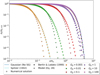 |
Fig. 2 Vertical profile of gas for different Toomre parameters when the dust component is disregarded. Specifically, we compare the numerical solution of Eq. (12) with the BL model and our model Eq. (28). |
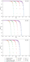 |
Fig. 3 Vertical profile of dust density for different gas Toomre parameters, Qg, and relative dust temperature, ξ. Specifically, we compare the numerical solution with our model Eq. (16). Additionally, we added the limiting cases of the Fromang and Nelson profile, which is valid in the absence of SG, and the exact solution that we derived (Eq. (13)), which is valid for massive gas discs. |
3.3 Spitzer and Bertin–Lodato models: a discussion on boundary conditions
In this section, we are concerned with the hydrostatic equilibrium of gas in the absence of dust:
![\[{\widetilde c_g}^2{\partial _{zz}}\ln \left( {{\rho _g}} \right) = - \Omega _K^2 - 4\pi G{\rho _g}.\]](/articles/aa/full_html/2025/05/aa53434-24/aa53434-24-eq50.png) (17)
(17)
As for any differential equation, this hydrostatic equilibrium is necessarily completed by boundary conditions satisfied by the scalar field and its derivative, which ensure the uniqueness of the solution. The Von Neumann condition is straightforward since the density is expected to reach its maximum value at the midplane, which translates to ∂zρg(z = 0) = 0. The Dirichlet condition is set equivalently either by a simple boundary condition in the midplane or by a coherent condition such as the one proposed in Eq. (10). We call this condition coherent because the surface density will affect the scale height definition, which in turn affects the surface density. Further, the condition defined by Eq. (10) implies the integrability of the density, which means that it should vanish at infinity while maintaining approximately a constant value close to the midplane. In other words, when ‘seen’ from large heights, the gas density can be considered as a Dirac delta function at the disc midplane. Consequently, at large heights, the gas stratification is simply governed by the star contribution and the gravity of a thin layer, causing the density to adopt the classic Gaussian profile with an absolute value correction. All of these clarifications can be summarised as follows:
![\[\left\{ {\begin{array}{*{20}{l}} {{\rho _g}(z = 0)}& = &{{\rho _{g,{\rm{mid}}}}}&{{\rm{or}}\quad {\rm{Eq}}.(10)}\\ {\mathop {\lim }\limits_{z \to \infty } {\rho _g}(z)}& \simeq &{{\rho _{g,{\rm{mid}}}}\exp \left( { - \frac{1}{2}{{\left( {\frac{z}{{{H_g}}}} \right)}^2} - \frac{{2|z|}}{{{Q_g}{H_g}}}} \right)}&{}\\ {{\partial _z}{\rho _g}(z = 0)}& = &0&. \end{array}} \right.\]](/articles/aa/full_html/2025/05/aa53434-24/aa53434-24-eq51.png) (18)
(18)
The model of BL correctly captures the gravity terms close to the midplane (up to the second order) thanks to a constant, modified scale height, which in turn forbids asymptotic connection with the above asymptotic profile. Nevertheless, this model informs us about the length-scale on which the gravity of the star and the disc prevail before connecting back to the Keplerian disc. In other words, ![\[H_g^{sg} = \sqrt {2/\pi } f({Q_g}){H_g}\]](/articles/aa/full_html/2025/05/aa53434-24/aa53434-24-eq52.png) is the length where the gravity of the disc cannot be disregarded. In the far-zone regime, after a few
is the length where the gravity of the disc cannot be disregarded. In the far-zone regime, after a few ![\[H_g^{sg}\]](/articles/aa/full_html/2025/05/aa53434-24/aa53434-24-eq53.png) , the disc can be thought of as being razor thin, and the standard Gaussian profile, augmented by the |z| correction, should be retrieved. The Spitzer model ignores these considerations because it assumes that the stellar term is zero when the Toomre parameter is very low. However, we have two objections. First, the star’s gravity must be present for large heights, more precisely beyond ∼Hg/Qg. Second, the Spitzer model can only disregard the star’s gravity for very low Qg values, below ∼0.1, at which the disc is expected to be highly unstable, making the assumption of hydrostatic equilibrium invalid.
, the disc can be thought of as being razor thin, and the standard Gaussian profile, augmented by the |z| correction, should be retrieved. The Spitzer model ignores these considerations because it assumes that the stellar term is zero when the Toomre parameter is very low. However, we have two objections. First, the star’s gravity must be present for large heights, more precisely beyond ∼Hg/Qg. Second, the Spitzer model can only disregard the star’s gravity for very low Qg values, below ∼0.1, at which the disc is expected to be highly unstable, making the assumption of hydrostatic equilibrium invalid.
We clarify that we are not questioning the models of Spitzer and BL, which remain valid within the framework of their hypotheses, namely, an approximate solution near the midplane. However, this detailed analysis on the boundary conditions has enabled us to reconsider the issue of stratification and refine the constraints, ultimately leading us to discover very precise and more general approximate solutions. We present these solutions in Sect. 4.
3.4 Summary
Our approximate model for gas and dust correctly matches the numerical and analytic solutions for Qg ≳ 1. For smaller Toomre parameters, the Gaussian model (Eq. (16)) tends towards the analytic solution that we found (Eq. (13)), but it deviates from ![\[z/{H_g} \mathbin{\lower.3ex\hbox{$\buildrel>\over {\smash{\scriptstyle\sim}\vphantom{_x}}$}} 4\sqrt {{Q_g}} \]](/articles/aa/full_html/2025/05/aa53434-24/aa53434-24-eq54.png) and z/Hd ≳ 3Qg for gas and dust profiles, respectively. However this is of little importance since at these heights, the density of gas and dust can be considered negligible compared to the midplane values.
and z/Hd ≳ 3Qg for gas and dust profiles, respectively. However this is of little importance since at these heights, the density of gas and dust can be considered negligible compared to the midplane values.
The stratifications found in this section are valid only in the limit where the gravitational contribution of dust can be disregarded. However, this assumption might not always hold true, considering that the observed low quantity of dust mass in Class II discs might not adequately account for the mass of discovered exoplanets (Ansdell et al. 2016; Manara et al. 2018; Mulders et al. 2021). This disagreement may imply the presence of more dust in discs than initially anticipated. Further, it is often considered that dust SG should be disregarded because of the low dust-to-gas column density ratio, Z = Σd/Σg, inferred from the interstellar medium. Nonetheless, we firmly believe that the appropriate measure for quantifying dust SG in the vertical orientation should be the dust-to-gas volume density ratio, ![\[{\rho _d}/{\rho _g} \simeq \frac{{{\Sigma _d}}}{{{\Sigma _g}}}\frac{{{H_g}}}{{{H_d}}}\]](/articles/aa/full_html/2025/05/aa53434-24/aa53434-24-eq55.png) . This quantity could be substantial for highly settled dust, a common occurrence frequently observed in PPDs (Pinte et al. 2016; Villenave et al. 2020, 2022). Finally, disc masses derived from (sub-)millimetre fluxes are underestimated compared to SED-inferred masses (Ballering & Eisner 2019; Ribas et al. 2020). This is further strengthened by the work of Vorobyov et al. (2024), who calculated the synthetic dust mass of a known numerical model. They found that the inferred mass from the observational estimates was two orders of magnitude smaller than the actual value, supporting the idea of a hidden dust reservoir within the disc. All aspects raised in this paragraph reinforce the importance of considering dust SG, and they prompted us to incorporate it into our analysis in the following section with a simpler assumption on the stopping time.
. This quantity could be substantial for highly settled dust, a common occurrence frequently observed in PPDs (Pinte et al. 2016; Villenave et al. 2020, 2022). Finally, disc masses derived from (sub-)millimetre fluxes are underestimated compared to SED-inferred masses (Ballering & Eisner 2019; Ribas et al. 2020). This is further strengthened by the work of Vorobyov et al. (2024), who calculated the synthetic dust mass of a known numerical model. They found that the inferred mass from the observational estimates was two orders of magnitude smaller than the actual value, supporting the idea of a hidden dust reservoir within the disc. All aspects raised in this paragraph reinforce the importance of considering dust SG, and they prompted us to incorporate it into our analysis in the following section with a simpler assumption on the stopping time.
4 Constant stopping time and gravitational contribution of dust
The constraint of a vertical dependence on the stopping time is very restrictive and complicates the resolution of the gas hydrostatic equation and transport equation for dust. Thus, in this section, we use the simple assumption τf = τf,mid, which permits us to rearrange the hydrostatic equations in a symmetric way where both gas sound speed and dust diffusivity are constant:
![\[\left\{ {\begin{array}{*{20}{c}} {{\rm{ }}{{\widetilde c}_g}^2{\partial _{zz}}\ln \left( {{\rho _g}} \right)}&{ = - \Omega _K^2 - 4\pi G\left( {{\rho _g} + {\rho _d}} \right)}\\ {{\rm{ }}{{\widetilde c}_d}^2{\partial _{zz}}\ln \left( {{\rho _d}} \right)}&{ = - \Omega _K^2 - 4\pi G\left( {{\rho _g} + {\rho _d}} \right)} \end{array}.} \right.\]](/articles/aa/full_html/2025/05/aa53434-24/aa53434-24-eq56.png) (19)
(19)
Here, ![\[{\widetilde c_d} = \xi /\sqrt {{\xi ^2} + 1} {\mkern 1mu} {c_{d,{\rm{mid}}}}\]](/articles/aa/full_html/2025/05/aa53434-24/aa53434-24-eq57.png) is an effective dust sound speed.
is an effective dust sound speed.
4.1 The approximated solution
We emphasise that the primary challenge in solving Eq. (19) lies in the coupled non-linear nature of the differential equations. More importantly, the simultaneous management of different scales presents a significant obstacle. For instance, considering the gas alone, we can quickly distinguish at least three possible height scales: the pressure scale height (Hg), the scale height of the influence of the gas mass (∼QgHg), and the scale height of the influence of dust mass (∼Qd Hg). For the latter, we further anticipate a weighting factor that depends on the relative temperature, ![\[\widetilde \xi = {\widetilde c_g}/{\widetilde c_{d,{\rm{mid}}}}\]](/articles/aa/full_html/2025/05/aa53434-24/aa53434-24-eq58.png) , which is not trivial at first sight. The presence of these different scale heights makes the resolution particularly difficult and precludes for bi-fluids the use of the method employed by Bertin & Lodato (1999), as detailed in Appendix C. We highlight that in this work we use
, which is not trivial at first sight. The presence of these different scale heights makes the resolution particularly difficult and precludes for bi-fluids the use of the method employed by Bertin & Lodato (1999), as detailed in Appendix C. We highlight that in this work we use
![\[{Q_d} = \frac{{{{\widetilde c}_d}{\Omega _K}}}{{\pi G{\Sigma _d}}} = \sqrt {\frac{{ - {\Omega _z}}}{{{\alpha _z} + (1 + {\alpha _z}){\mkern 1mu} St}}} \;\frac{{{\Sigma _g}}}{{{\Sigma _d}}}{Q_g},\]](/articles/aa/full_html/2025/05/aa53434-24/aa53434-24-eq59.png) (20)
which aligns with the definition of Klahr & Schreiber (2021) in the limit of small vertical diffusivity compared to the Stokes number.
(20)
which aligns with the definition of Klahr & Schreiber (2021) in the limit of small vertical diffusivity compared to the Stokes number.
As in the previous section, the set of Eq. (19) can be ultimately reduced to a single equation with a transformation that permits one to retrieve the dust profile:
![\[\left\{ {\begin{array}{*{20}{l}} {{{\widetilde c}_g}^2{\partial _{zz}}\ln {\mkern 1mu} \left( {\frac{{{\rho _g}}}{{{\rho _{g,{\rm{mid}}}}}}} \right)}& = &{ - \Omega _K^2}\\ {}&{}&{ - 4\pi G\left[ {{\rho _g} + {\rho _{d,{\rm{mid}}}}{\mkern 1mu} {{\left( {\frac{{{\rho _g}}}{{{\rho _{g,{\rm{mid}}}}}}} \right)}^{{{\widetilde \xi }^2}}}} \right]}\\ {{\rho _d} = {\rho _{d,{\rm{mid}}}}{{\left( {\frac{{{\rho _g}}}{{{\rho _{g,{\rm{mid}}}}}}} \right)}^{{{\widetilde \xi }^2}}}}&{}&{} \end{array},} \right.\]](/articles/aa/full_html/2025/05/aa53434-24/aa53434-24-eq60.png) (21)
where ρi,mid is the midplane density of phase i. Equation (21) is essentially a 1D Liouville equation (Liouville 1853) with a constant term and two exponential non-linearities. Even when the star’s gravity is negligible, ΩK = 0, solving Eq. (21) is a challenging endeavour that represents an active field of research in mathematical physics (Mancas et al. 2018). To our knowledge, there are very few exact solutions available, and they unfortunately do not apply to our specific problem. Furthermore, we are also interested in the smooth transition between a Keplerian disc into a self-gravitating disc dominated by gas, by dust, or by both phases. This implies that we cannot neglect any term in Eq. (21). However, motivated by the underlying structure of new analytical solutions to Eq. (19) in specific cases (see Appendix D) and the method that we developed in Appendix E, we managed to build an accurate approximate solution that is valid for all relative temperatures and in all regimes of SG, from Keplerian discs to massive discs made of gas and/or dust and that respect the physical boundary conditions mentioned in Sect. 3.3. This new approximated solution is
(21)
where ρi,mid is the midplane density of phase i. Equation (21) is essentially a 1D Liouville equation (Liouville 1853) with a constant term and two exponential non-linearities. Even when the star’s gravity is negligible, ΩK = 0, solving Eq. (21) is a challenging endeavour that represents an active field of research in mathematical physics (Mancas et al. 2018). To our knowledge, there are very few exact solutions available, and they unfortunately do not apply to our specific problem. Furthermore, we are also interested in the smooth transition between a Keplerian disc into a self-gravitating disc dominated by gas, by dust, or by both phases. This implies that we cannot neglect any term in Eq. (21). However, motivated by the underlying structure of new analytical solutions to Eq. (19) in specific cases (see Appendix D) and the method that we developed in Appendix E, we managed to build an accurate approximate solution that is valid for all relative temperatures and in all regimes of SG, from Keplerian discs to massive discs made of gas and/or dust and that respect the physical boundary conditions mentioned in Sect. 3.3. This new approximated solution is
![\[\left\{ {\begin{array}{*{20}{l}} {{\rho _g}(r,z) = {\rho _{g,{\rm{mid}}}}\exp \left[ { - \frac{1}{2}{{\left( {\frac{z}{{{H_g}}}} \right)}^2}} \right.}&{ - \sqrt {\frac{\pi }{2}} \frac{1}{{Q_g^{sg}}}{\rm{ }}\Theta \left( {\frac{z}{{H_g^{sg}}}} \right)}\\ {}&{\left. { - \sqrt {\frac{\pi }{2}} \frac{1}{{{{\widetilde \xi }^2}Q_d^{sg}}}{\rm{ }}\Theta \left( {\frac{z}{{H_d^{sg}}}} \right)} \right]}\\ {{\rho _d}(r,z) = {\rho _{d,{\rm{mid}}}}{{\left[ {{\rho _g}/{\rho _{g,{\rm{mid}}}}} \right]}^{{{\widetilde \xi }^2}}}}&{} \end{array}} \right.\]](/articles/aa/full_html/2025/05/aa53434-24/aa53434-24-eq61.png) (22)
with
(22)
with
![\[\left\{ {\begin{array}{*{20}{l}} {\Theta \left( z \right)}& = &{\exp \left( { - \frac{1}{2}{z^2}} \right) + \sqrt {\frac{\pi }{2}} {\mkern 1mu} z{\mkern 1mu} {\rm{erf}}\left( {\frac{z}{{\sqrt 2 }}} \right) - 1}\\ {{k_1}}& = &{1{\mkern 1mu} /\sqrt {1 + \sqrt {\frac{\pi }{2}} \left( {\frac{1}{{Q_g^{3D}}} + \frac{1}{{Q_d^{3D}}}} \right)} }\\ {H_i^{sg}}& = &{{k_1}{H_i}}\\ {Q_i^{3D}}& = &{\sqrt {\frac{\pi }{2}} \frac{{\Omega _K^2}}{{{\pi ^2}G{\rho _{i,{\rm{mid}}}}}}}\\ {Q_i^{sg}}& = &{Q_i^{3D}{{\left( {{\Omega _{sg}}/{\Omega _K}} \right)}^2}}\\ {{\Omega _{sg}}}& = &{{\Omega _K}/{k_1}} \end{array},} \right.\]](/articles/aa/full_html/2025/05/aa53434-24/aa53434-24-eq62.png) (23)
(23)
Where ![\[\widetilde \xi = {\widetilde c_g}/{\widetilde c_{d,{\rm{mid}}}}\]](/articles/aa/full_html/2025/05/aa53434-24/aa53434-24-eq63.png) , ‘erf’ is the error function and the function f is the same as the one obtained with the BL method. We emphasise that our definition of the 3D Toomre parameter,
, ‘erf’ is the error function and the function f is the same as the one obtained with the BL method. We emphasise that our definition of the 3D Toomre parameter, ![\[Q_i^{3D}\]](/articles/aa/full_html/2025/05/aa53434-24/aa53434-24-eq64.png) , slightly differs from the one proposed by Mamatsashvili & Rice (2010), that is, by a factor of approximately 1.6. However, we believe our definition is correct because, for negligible SG in the vertical direction, it aligns with the 2D Toomre parameter. Without going into further detail, we observed that our problem is governed by three height scales, the interpretation of which is provided in Sect. 4.3. It is curious that the relative temperature
, slightly differs from the one proposed by Mamatsashvili & Rice (2010), that is, by a factor of approximately 1.6. However, we believe our definition is correct because, for negligible SG in the vertical direction, it aligns with the 2D Toomre parameter. Without going into further detail, we observed that our problem is governed by three height scales, the interpretation of which is provided in Sect. 4.3. It is curious that the relative temperature ![\[\widetilde \xi \]](/articles/aa/full_html/2025/05/aa53434-24/aa53434-24-eq65.png) does not explicitly affect any physical quantity establishing the settling, such as
does not explicitly affect any physical quantity establishing the settling, such as ![\[H_i^{sg}\]](/articles/aa/full_html/2025/05/aa53434-24/aa53434-24-eq66.png) or
or ![\[Q_i^{3D}\]](/articles/aa/full_html/2025/05/aa53434-24/aa53434-24-eq67.png) . However, it could be indirectly present in the ρi,mid definition. It seems that its unique role is to act as a conversion parameter between the gas and dust layering. Finally, in a fairly convenient manner, the Θ function satisfies the next relation at infinity:
. However, it could be indirectly present in the ρi,mid definition. It seems that its unique role is to act as a conversion parameter between the gas and dust layering. Finally, in a fairly convenient manner, the Θ function satisfies the next relation at infinity:
![\[\mathop {\lim }\limits_{z \to \pm \infty } \Theta \left( {\frac{z}{{H_g^{sg}}}} \right) = \sqrt {\frac{\pi }{2}} \frac{{|z|}}{{H_g^{sg}}},\]](/articles/aa/full_html/2025/05/aa53434-24/aa53434-24-eq68.png) (24)
which makes ρg adopt the asymptotic behaviour expected from Sect. 3.3.
(24)
which makes ρg adopt the asymptotic behaviour expected from Sect. 3.3.
4.2 Validation
For validating the accuracy of our solution, there are two techniques. The first involves comparing our results with analytic and approximate solutions in limiting cases, such as those presented in Appendices C and D. While this validation is left to the reader, we would like to confirm that we have verified that close to the midplane, our solution yields the scale heights associated with all limiting cases. Particularly, when dust is absent, a Taylor expansion up to a second order in function Θ in Eq. (22) permits retrieval of the BL model. The second validation method is based on numerical comparison, which we discuss next.
We estimated the accuracy of our self-gravitating bi-fluid model. To do so, we quantified the deviation between the numerical solution and our model by estimating the following L2 norm:
![\[||\varepsilon |{|_2} = \frac{1}{{{N_z}}}{\left( {\sum\limits_{i = 0}^{{N_z}} {{{\left| {\frac{{{\rho _{g,{\rm{model}}}}({z_i})}}{{{\rho _{g,{\rm{num}}}}({z_i})}} - 1} \right|}^2}} ,} \right)^{1/2}}\]](/articles/aa/full_html/2025/05/aa53434-24/aa53434-24-eq69.png) (25)
where Nz is the number of points. In Fig. 4, we compare the numerical solution of Eq. (19) with our approximated solution (Eq. (22)) for different relative temperatures
(25)
where Nz is the number of points. In Fig. 4, we compare the numerical solution of Eq. (19) with our approximated solution (Eq. (22)) for different relative temperatures ![\[\widetilde \xi \]](/articles/aa/full_html/2025/05/aa53434-24/aa53434-24-eq70.png) and different gas
and different gas ![\[(Q_g^{3D})\]](/articles/aa/full_html/2025/05/aa53434-24/aa53434-24-eq71.png) and dust
and dust ![\[\left( {Q_d^{3D}} \right)\]](/articles/aa/full_html/2025/05/aa53434-24/aa53434-24-eq72.png) Toomre parameters. Specifically, in the left column we plot the vertical profiles of gas, and in the right column, we present a map of the L2 norm for gas and dust Toomre parameters, ranging from 0.01 to 100, and a fixed relative temperature. Specifically, for each triplet
Toomre parameters. Specifically, in the left column we plot the vertical profiles of gas, and in the right column, we present a map of the L2 norm for gas and dust Toomre parameters, ranging from 0.01 to 100, and a fixed relative temperature. Specifically, for each triplet ![\[(Q_g^{3D},Q_d^{3D},{\rm{ }}\widetilde \xi )\]](/articles/aa/full_html/2025/05/aa53434-24/aa53434-24-eq73.png) , we employ Nz = 50 000 points spaced evenly in a log scale in the range
, we employ Nz = 50 000 points spaced evenly in a log scale in the range ![\[z/H_g^{sg} \in [1/(100{\rm{ }}\widetilde \xi ),5]\]](/articles/aa/full_html/2025/05/aa53434-24/aa53434-24-eq74.png) 2. Using a log scale enabled us to capture both small- and large-scale variations associated with dust and gas. We found that the relative deviation is on the order of 10−4 and 10−3 for all of our parameters. Such low deviations confirm that our approximated solution is a generally correct description for self-gravitating discs composed of gas and dust. In the next section, we provide a physical interpretation of all quantities involved in the gas-dust layering that we just found.
2. Using a log scale enabled us to capture both small- and large-scale variations associated with dust and gas. We found that the relative deviation is on the order of 10−4 and 10−3 for all of our parameters. Such low deviations confirm that our approximated solution is a generally correct description for self-gravitating discs composed of gas and dust. In the next section, we provide a physical interpretation of all quantities involved in the gas-dust layering that we just found.
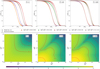 |
Fig. 4 Comparison between the numerical solution of Eq. (19) and our approximated solution (Eq. (22)) for different Toomre parameters of gas |
![\[(\$ Q_g^{3D}\$ )\]](/articles/aa/full_html/2025/05/aa53434-24/aa53434-24-eq75.png)
![\[(\$ Q_d^{3D}\$ )\]](/articles/aa/full_html/2025/05/aa53434-24/aa53434-24-eq76.png)
![\[{\rm{(}}\widetilde \xi {\rm{)}}\]](/articles/aa/full_html/2025/05/aa53434-24/aa53434-24-eq77.png)
4.3 Physical interpretation
In this paragraph, we provide a physical interpretation of the quantities involved in the stratification described by Eqs. (22)–(23). We primarily focus on the gas length scales, as the dust length scales can be directly obtained by multiplying by ![\[\widetilde \xi \]](/articles/aa/full_html/2025/05/aa53434-24/aa53434-24-eq78.png) . The first noticeable scale is the standard pressure scale height, Hg, whose perceptible role is to account for the star gravity and to allow for a connection with the background Gaussian layering. In the presence of the SG of both phases,
. The first noticeable scale is the standard pressure scale height, Hg, whose perceptible role is to account for the star gravity and to allow for a connection with the background Gaussian layering. In the presence of the SG of both phases, ![\[H_g^{sg}\]](/articles/aa/full_html/2025/05/aa53434-24/aa53434-24-eq79.png) and
and ![\[H_d^{sg}\]](/articles/aa/full_html/2025/05/aa53434-24/aa53434-24-eq80.png) represent the lengths over which the gravity generated by the gas and dust profiles act, respectively. In other words, these are the widths of the gas and dust layers. Specifically, in the absence of dust,
represent the lengths over which the gravity generated by the gas and dust profiles act, respectively. In other words, these are the widths of the gas and dust layers. Specifically, in the absence of dust, ![\[H_g^{sg}\]](/articles/aa/full_html/2025/05/aa53434-24/aa53434-24-eq81.png) equals the length scale of the BL biased Gaussian model (see Eq. (15)). In particular, these scale height definitions involve the quantity k1 provided by Eq. (23), which is constructed as a combination of the root mean square and harmonic average of the Toomre parameters of the gas and dust, which also includes the star contribution (the unity term). Somehow, the writing of k1 shows the competition between all terms for dominating the vertical settling. More interestingly, the harmonic average of the gas and dust Toomre parameters naturally emerges as
equals the length scale of the BL biased Gaussian model (see Eq. (15)). In particular, these scale height definitions involve the quantity k1 provided by Eq. (23), which is constructed as a combination of the root mean square and harmonic average of the Toomre parameters of the gas and dust, which also includes the star contribution (the unity term). Somehow, the writing of k1 shows the competition between all terms for dominating the vertical settling. More interestingly, the harmonic average of the gas and dust Toomre parameters naturally emerges as
![\[Q_{{\rm{bi - fluid}}}^{3D} = {\left( {\frac{1}{{Q_g^{3D}}} + \frac{1}{{Q_d^{3D}}}} \right)^{ - 1}},\]](/articles/aa/full_html/2025/05/aa53434-24/aa53434-24-eq82.png) (26)
and it is immediately interpreted as the general Toomre parameter for a bi-fluid self-gravitating disc when dust is embedded in a turbulent gaseous environment. An interesting property of this harmonic average is that when the mass of one of the two phases predominates, the bi-fluid Toomre parameter adopts its value. We strongly believe that this definition of the Toomre parameter, which naturally emerges from first principles, is the appropriate quantity for quantifying SG in bi-fluid systems.
(26)
and it is immediately interpreted as the general Toomre parameter for a bi-fluid self-gravitating disc when dust is embedded in a turbulent gaseous environment. An interesting property of this harmonic average is that when the mass of one of the two phases predominates, the bi-fluid Toomre parameter adopts its value. We strongly believe that this definition of the Toomre parameter, which naturally emerges from first principles, is the appropriate quantity for quantifying SG in bi-fluid systems.
We propose another axis of analysis based on differential rotation. If all terms inside the exponential of Eq. (22) are factored by z2/2, we can rewrite the gas density profile as a simple Gaussian with a scale height defined by ![\[H_g^{sg}(z) = {c_g}/{\Omega _{sg}}(z)\]](/articles/aa/full_html/2025/05/aa53434-24/aa53434-24-eq83.png) , where Ωsg acts as a modified differential rotation due to SG. Indeed, everything happens as if the disc were more massive close to the midplane. The expression for the modified rotation due to SG is
, where Ωsg acts as a modified differential rotation due to SG. Indeed, everything happens as if the disc were more massive close to the midplane. The expression for the modified rotation due to SG is
![\[\frac{{{\Omega _{sg}}(z)}}{{{\Omega _K}}} = \sqrt {1 + \sqrt {2\pi } {{\left( {\frac{{{H_g}}}{z}} \right)}^2}\left[ {\frac{1}{{Q_g^{sg}}}\Theta \left( {\frac{z}{{H_g^{sg}}}} \right) + \frac{1}{{{{\widetilde \xi }^2}Q_d^{sg}}}\Theta \left( {\frac{z}{{H_d^{sg}}}} \right)} \right]} .\]](/articles/aa/full_html/2025/05/aa53434-24/aa53434-24-eq84.png) (27)
(27)
It is important to note that SG influences the dynamics of massive discs, causing significant deviations from the Keplerian rotation profile (Lodato et al. 2023; Veronesi et al. 2024; Speedie et al. 2024). However, in our framework, the above differential rotation is a theoretical construct that helps us understand the problem from a different perspective, but it is not directly observable nor related to the kinematic signatures of SG. As explained in Sect. 3.1, our study focuses solely on vertical effects. To establish a clear connection between the rotation profile and vertical stratification of massive discs, we would need to remove the slab approximation. Indeed, this approximation assumes that the SG of a volume element is influenced only by the mass distribution at that specific location. Nonetheless, the reduction in scale height due to SG also decreases the pressure support, likely impacting the rotation profile (Nelson et al. 2013, Eq. (13)). In Fig. 5, we depict the above self-gravitating frequency for different dust Toomre parameters and relative temperatures. For all cases, we fixed ![\[Q_g^{3D} = 0.5\]](/articles/aa/full_html/2025/05/aa53434-24/aa53434-24-eq85.png) , which is the standard value found in 3D simulations where the gravitational instability of gas is self-regulated for slow cooling. We found subsequent deviations to the Keplerian frequency that range between two to five times the Keplerian frequency. In some cases, these deviations can be felt well above the midplane, up to five pressure scale heights. Our plots of the self-gravitating frequency also show that our problem is governed by various scale heights. This is particularly explicit for the curve
, which is the standard value found in 3D simulations where the gravitational instability of gas is self-regulated for slow cooling. We found subsequent deviations to the Keplerian frequency that range between two to five times the Keplerian frequency. In some cases, these deviations can be felt well above the midplane, up to five pressure scale heights. Our plots of the self-gravitating frequency also show that our problem is governed by various scale heights. This is particularly explicit for the curve ![\[(Q_d^{3D},\widetilde \xi ) = (0.5,100)\]](/articles/aa/full_html/2025/05/aa53434-24/aa53434-24-eq86.png) , where we observed that at z/Hg ≃ 10−3 and z/Hg ≃ 10−1, the slope of the curve suddenly changes. This behaviour can mostly be seen for high values of the relative temperature. Finally, at the midplane (z = 0), the ratio Ωsg/ΩK equals 1/k1. Based on this result, we propose in the next paragraph a possible redefinition of the Toomre parameters governing our problem.
, where we observed that at z/Hg ≃ 10−3 and z/Hg ≃ 10−1, the slope of the curve suddenly changes. This behaviour can mostly be seen for high values of the relative temperature. Finally, at the midplane (z = 0), the ratio Ωsg/ΩK equals 1/k1. Based on this result, we propose in the next paragraph a possible redefinition of the Toomre parameters governing our problem.
In Eq. (23), we introduced self-gravitating Toomre parameters: ![\[Q_i^{sg}\]](/articles/aa/full_html/2025/05/aa53434-24/aa53434-24-eq90.png) . It can be readily shown that these parameters align with the standard definition for light discs since in this limit we have Ωsg → ΩK. In this context, it is important to recall that the Toomre stability criterion, Qg > 1, indicates the condition under which razor thin discs are stable against perturbations (Toomre 1964). An intriguing aspect of our definitions is the possibility of a situation where, for instance, Qg < 1 for the gas alone, but
. It can be readily shown that these parameters align with the standard definition for light discs since in this limit we have Ωsg → ΩK. In this context, it is important to recall that the Toomre stability criterion, Qg > 1, indicates the condition under which razor thin discs are stable against perturbations (Toomre 1964). An intriguing aspect of our definitions is the possibility of a situation where, for instance, Qg < 1 for the gas alone, but ![\[Q_g^{sg} > 1\]](/articles/aa/full_html/2025/05/aa53434-24/aa53434-24-eq91.png) . In particular, we have
. In particular, we have ![\[Q_g^{sg} \xrightarrow[Q_g\rightarrow 0]{} \sqrt{\pi/2}\]](/articles/aa/full_html/2025/05/aa53434-24/aa53434-24-eq92.png) . This raises the question of whether the self-gravitating Toomre parameter has a physical meaning or not and, specifically, whether the vertical SG acts as a potential stabilising term. Currently, this is unclear and cannot be analytically demonstrated. Indeed, the proof of Toomre stability criterion relies on the thin disc approximation, which overlooks the vertical stratification of the disc and thus loses information about modified scale heights or differential rotation. To determine if
. This raises the question of whether the self-gravitating Toomre parameter has a physical meaning or not and, specifically, whether the vertical SG acts as a potential stabilising term. Currently, this is unclear and cannot be analytically demonstrated. Indeed, the proof of Toomre stability criterion relies on the thin disc approximation, which overlooks the vertical stratification of the disc and thus loses information about modified scale heights or differential rotation. To determine if ![\[Q_i^{sg}\]](/articles/aa/full_html/2025/05/aa53434-24/aa53434-24-eq93.png) plays a role in disc stability, rather than Qi, it would be necessary to demonstrate the Toomre stability criterion using a more sophisticated assumption than ΔΦ = 4πGΣd(z).
plays a role in disc stability, rather than Qi, it would be necessary to demonstrate the Toomre stability criterion using a more sophisticated assumption than ΔΦ = 4πGΣd(z).
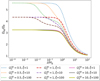 |
Fig. 5 Self-gravitating differential rotation in a marginally gas-stable disc ( |
![\[(Q_g^{3D} = 0.5)\]](/articles/aa/full_html/2025/05/aa53434-24/aa53434-24-eq87.png)
![\[(Q_d^{3D})\]](/articles/aa/full_html/2025/05/aa53434-24/aa53434-24-eq88.png)
![\[{\rm{(}}\widetilde \xi {\rm{)}}\]](/articles/aa/full_html/2025/05/aa53434-24/aa53434-24-eq89.png)
4.4 A closed form for single fluid discs
When a single fluid is present, it is further possible to explicitly relate the midplane density with k1 and the surface density Σg (see Appendix E.1). With this result, the gas density vertical profile is
![\[{\rho _g}(r,z) = \frac{{{\Sigma _g}}}{{\sqrt {2\pi } H_g^{sg}}}\exp \left[ { - \frac{1}{2}{{\left( {\frac{z}{{{H_g}}}} \right)}^2} - \sqrt {\frac{\pi }{2}} \frac{1}{{Q_g^{sg}}}{\rm{ }}\Theta \left( {\frac{z}{{H_g^{sg}}}} \right)} \right],\]](/articles/aa/full_html/2025/05/aa53434-24/aa53434-24-eq94.png) (28)
with
(28)
with
![\[\left\{ {\begin{array}{*{20}{l}} {H_g^{sg}}& = &{\sqrt {\frac{2}{\pi }} {H_g}f({Q_g})}\\ {Q_g^{sg}}& = &{\sqrt {\frac{\pi }{2}} \frac{{{Q_g}}}{{f({Q_g})}}} \end{array}.} \right.\]](/articles/aa/full_html/2025/05/aa53434-24/aa53434-24-eq95.png) (29)
(29)
In particular, this scale height definition involves the quantity ![\[\sqrt{2/\pi} f(Q_g)\]](/articles/aa/full_html/2025/05/aa53434-24/aa53434-24-eq96.png) , which weights non-linearly the effect of SG in the stratification. For light discs specifically, the above quantity equals unity, while it equals
, which weights non-linearly the effect of SG in the stratification. For light discs specifically, the above quantity equals unity, while it equals ![\[\sqrt{2/\pi} Q_g\]](/articles/aa/full_html/2025/05/aa53434-24/aa53434-24-eq97.png) for massive discs. In Fig. 2, we compare our approximate solution with the BL model and numerical solution in the case of a single fluid. Across the entire range of z values and Toomre parameters, our model aligns almost perfectly with the numerical solution. In contrast, the BL model exhibits limitations at small Toomre parameters. We emphasise that our solution tends asymptotically towards the standard Gaussian corrected by an absolute value term, which reinforces the robustness of our solution (see Sect. 3.3). Specifically, for strong SG, we obtain
for massive discs. In Fig. 2, we compare our approximate solution with the BL model and numerical solution in the case of a single fluid. Across the entire range of z values and Toomre parameters, our model aligns almost perfectly with the numerical solution. In contrast, the BL model exhibits limitations at small Toomre parameters. We emphasise that our solution tends asymptotically towards the standard Gaussian corrected by an absolute value term, which reinforces the robustness of our solution (see Sect. 3.3). Specifically, for strong SG, we obtain ![\[\log(\rho_g) \xrightarrow[z\rightarrow \infty]{} -\frac{1}{2} (z/H_g)^2 - \frac{\pi}{2} |z|/(Q_g H_g)\]](/articles/aa/full_html/2025/05/aa53434-24/aa53434-24-eq98.png) .
.
We believe that only the self-gravitating scale heights can be probed by astronomical observations and that this could permit indirect access to disc masses. We address this point in the next section.
5 Connecting theory to observations
In this section, we explore the possibility of inferring disc masses through the stratification and, more precisely, the scale heights exhibited in previous sections. Given the non-standard character of the profiles derived in this work, it is first necessary to define what a dust-to-gas scale height entails in such a case.
5.1 A generic definition of dust-to-gas scale height
The definition of the dust-to-gas scale height ratio is an interesting issue that needs clarification, especially given the complex profiles exhibited in this work. Finding a general definition of scale heights that applies from Gaussian profiles to non-standard profiles, such as the intricate exponential exhibited in Eq. (16), can be challenging. Already, the simple sech2 profile faced this issue, leading Klahr & Schreiber (2021, Sect. 2.1) to revise their initial scale height definition. In this section, we propose a revision of the dust-to-gas scale height that is valid independently of the form of the profile and therefore applicable even in the presence of complex vertical profiles.
We first investigated a possible definition for the complex profile exhibited in Eq. (16). Given that both phases are subject to the same vertical forces, the dust-to-gas ratio is simply defined as the ratio of the dust diffusivity by the gas sound speed. However, these last quantities are not defined simply and are possibly z dependent for sophisticated profiles. For the case of dust, the first step would be to define the correct diffusivity. To do so, it is necessary to write its hydrostatic equilibrium in a symmetric way with respect to the one of gas:
![\[{\widetilde c_d}^2(z){\mkern 1mu} {\partial _{zz}}\ln \left( {{\rho _d}} \right) = - \Omega _K^2 - 4\pi G{\rho _g},\]](/articles/aa/full_html/2025/05/aa53434-24/aa53434-24-eq99.png) (30)
where
(30)
where
![\[{\widetilde c_d}(z) = \frac{{{c_d}(z)}}{{\sqrt {1 + {{({c_d}(z)/{{\widetilde c}_g})}^2}} }} = \sqrt {\frac{{{X_g}(z)}}{{{\xi ^2} + {X_g}(z)}}} {\rm{ }}{\widetilde c_g}\]](/articles/aa/full_html/2025/05/aa53434-24/aa53434-24-eq100.png) (31)
is a z-dependent effective dust diffusivity and the quantity Xg(z) = ρg(z)/ρg,mid is the normalised gas density. The next step consisted of finding a convenient average method. A naïve approach would consist of integrating the above expression from negative to positive infinity and multiplying it with a convenient normalisation factor. However, this necessarily results in a dust diffusivity that diverges to infinity for ξ2 = St(1 + αz)/αz →0, which is inconsistent. To address this, we found using a density weighted average to be more appropriate for defining the mean dust diffusivity:
(31)
is a z-dependent effective dust diffusivity and the quantity Xg(z) = ρg(z)/ρg,mid is the normalised gas density. The next step consisted of finding a convenient average method. A naïve approach would consist of integrating the above expression from negative to positive infinity and multiplying it with a convenient normalisation factor. However, this necessarily results in a dust diffusivity that diverges to infinity for ξ2 = St(1 + αz)/αz →0, which is inconsistent. To address this, we found using a density weighted average to be more appropriate for defining the mean dust diffusivity:
![\[{\langle {\rm{ }}{\widetilde c_i}\rangle _{{\rho _i}}} = \int\limits_{ - \infty }^\infty {{\rho _i}} (z){\rm{ }}{\widetilde c_i}(z){\mkern 1mu} dz\;/\int\limits_{ - \infty }^\infty {{\rho _i}} (z){\mkern 1mu} dz.\]](/articles/aa/full_html/2025/05/aa53434-24/aa53434-24-eq101.png) (32)
(32)
Finally, we defined the general dust-to-gas scale height ratio (valid for any profile of gas and dust) as the ratio of the density weighted dust diffusivity and density weighted gas sound speed:
![\[{H_d}/H_g^{sg}: = {\rm{ }}{\langle {\widetilde c_d}\rangle _{{\rho _d}}}/{\langle {\rm{ }}{\widetilde c_g}\rangle _{{\rho _g}}}.\]](/articles/aa/full_html/2025/05/aa53434-24/aa53434-24-eq102.png) (33)
(33)
It is important to note that this definition is valid only if both phases are subject to the same vertical forces. A clear benefit of the above definition is that it makes possible a generic definition of dust-to-gas scale height ratios that are valid for complex profiles, and at the same time, it makes the comparison of dust-to-gas scale height meaningful between different profiles, such as Gaussian, hyperbolic secant, and intricate exponentials. This definition also leaves the standard definition of dust-to-gas scale heights unchanged when the diffusion of dust and gas sound speed are space constants.
We applied the above definition to the profiles obtained in Sect. 3.2 and Sect. 4.1. According to our prescription, for Eq. (16), the dust-to-gas scale height ratio is
![\[\begin{array}{*{20}{l}} {{H_d}/H_g^{sg}}& = &{\int\limits_{ - \infty }^\infty {} \sqrt {\frac{{G(u)}}{{{\xi ^2} + G(u)}}} G(u)\exp \left( { - \frac{{{\xi ^2}}}{{G(u)}}} \right){\mkern 1mu} du{\mkern 1mu} /}\\ {}&{}&{\int\limits_{ - \infty }^\infty G (u)\exp \left( { - \frac{{{\xi ^2}}}{{G(u)}}} \right){\mkern 1mu} du,} \end{array}\]](/articles/aa/full_html/2025/05/aa53434-24/aa53434-24-eq103.png) (34)
(34)
With ![\[G(u)=e^{-{u^2}/2}\]](/articles/aa/full_html/2025/05/aa53434-24/aa53434-24-eq104.png) . In Fig. 6, we illustrate the relative difference (in percent) between the scale height ratio proposed by Dubrulle et al. (1995) and our revised finding in Eq. (34) for different turbulence strengths and Stokes numbers. We found notable differences only for strong stirring and large Stokes numbers. Our investigation revealed that the correction involving the turbulent gas pressure significantly contributes to these deviations. These conditions might be especially relevant in the context of gravitational instability, as simulations have demonstrated that the αS -parameter can approach values close to unity (Kratter et al. 2008). Next, we applied the definition outlined in Eq. (33) to Eq. (19). We obtained
. In Fig. 6, we illustrate the relative difference (in percent) between the scale height ratio proposed by Dubrulle et al. (1995) and our revised finding in Eq. (34) for different turbulence strengths and Stokes numbers. We found notable differences only for strong stirring and large Stokes numbers. Our investigation revealed that the correction involving the turbulent gas pressure significantly contributes to these deviations. These conditions might be especially relevant in the context of gravitational instability, as simulations have demonstrated that the αS -parameter can approach values close to unity (Kratter et al. 2008). Next, we applied the definition outlined in Eq. (33) to Eq. (19). We obtained
![\[\begin{array}{*{20}{l}} {H_d^{sg}/H_g^{sg}}&{ = {{\langle {\rm{ }}{{\widetilde c}_d}\rangle }_{{\rho _d}}}/{{\langle {\rm{ }}{{\widetilde c}_g}\rangle }_{{\rho _g}}}}\\ {}&{ = {\rm{ }}{{\widetilde c}_d}/{{\widetilde c}_g}}\\ {}&{ = \sqrt {\frac{{{\alpha _z}}}{{{\alpha _z} + \left( {1 + {\alpha _z}} \right){\rm{ St}}}}} }\\ {}&{ = \sqrt {\frac{1}{{1 + {\xi ^2}}}} } \end{array}.\]](/articles/aa/full_html/2025/05/aa53434-24/aa53434-24-eq105.png) (35)
(35)
In particular, when both phases are subject to the same vertical forces, as is the case here, the above ratio is a physical invariant. This relation holds true regardless of the presence of SG and is a revision of the formula by Dubrulle et al. (1995) that accounts for how gas turbulence affects not only dust but also its own scale height via a turbulent pressure. For weak stirring, αz ≪ 1, we retrieved the result of Dubrulle et al. (1995). However, for strong stirring, our revised finding in Eq. (35) deviates from the Dubrulle et al. (1995) relation, similar to how Eq. (34) deviates from their formula, namely for strong vertical stirring (αz ≃ 1).
Figure 7 illustrates the dust-to-gas scale height ratio as a function of ξ2 = (1 + αz)St/αz using both Eq. (35) and the more generally applicable proposed dust-to-gas scale height ratio of Eq. (34). For completeness, we added the three points that come from Fromang & Nelson (2009) simulations. We note that while their work originally plotted the dust-to-gas scale height ratio as a function of the Stokes number, we adapted it to be a function of ξ2 based on the rest of their data. First, we found no significant differences between our two prescriptions. Therefore, for simplicity, we recommend using the formula provided by Eq. (35) over that of Eq. (34). Second, we observed that the points from Fromang & Nelson (2009) fit our curves correctly, closely resembling the prescription of Dubrulle et al. (1995), with deviations appearing only at strong stirrings. Thus, it is unclear why the authors chose to fit their points with a power law instead of using the known prescription of Dubrulle et al. (1995). In summary, we believe that determining the dust-to-gas scale height solely as a function of the Stokes number provides incomplete and biased information. Instead, it is more appropriate to determine it as a function of ξ2 = (1 + αz)St/αz.
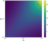 |
Fig. 6 Relative difference between the original relation of Dubrulle et al. (1995) and the revised versions that we propose in Eq. (34). The red solid lines show contour levels at 5%, 10%, and 20%. |
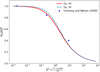 |
Fig. 7 Dust-to-gas ratio scale height as a function of the vertical diffusivity and Stokes number when the stopping time has a vertical profile (Eq. (34)) and when it is constant (Eq. (35)). |
5.2 Indirect mass estimation
As shown in Eq. (23), when accounting for SG, the dust and gas scale heights, ![\[H_i^{sg}\]](/articles/aa/full_html/2025/05/aa53434-24/aa53434-24-eq106.png) , show a symmetric relation with their respective ci terms and the k1 quantity, which contains information on the disc mass. Thus, independent measurements of both the scale height and the temperature, or vertical stirring, of the gas and the dust, respectively, could provide insights into the total disc mass. In this paragraph, we detail the procedure for the gas alone, which can be easily generalised when dust is present. First, it is necessary to obtain cg, which is readily accessible through the gas temperature. This allows for the computation of the standard pressure scale height, Hg. The gas temperature can also potentially be determined through dust temperature measurements, assuming thermodynamic equilibrium between the gas and dust. Second, the actual vertical scale height,
, show a symmetric relation with their respective ci terms and the k1 quantity, which contains information on the disc mass. Thus, independent measurements of both the scale height and the temperature, or vertical stirring, of the gas and the dust, respectively, could provide insights into the total disc mass. In this paragraph, we detail the procedure for the gas alone, which can be easily generalised when dust is present. First, it is necessary to obtain cg, which is readily accessible through the gas temperature. This allows for the computation of the standard pressure scale height, Hg. The gas temperature can also potentially be determined through dust temperature measurements, assuming thermodynamic equilibrium between the gas and dust. Second, the actual vertical scale height, ![\[H_g^{sg}\]](/articles/aa/full_html/2025/05/aa53434-24/aa53434-24-eq107.png) , which is the real quantity that can be accessed by the data, should be measured by an independent method. Together, these two scale heights enable the computation of the gas Toomre parameter of the disc:
, which is the real quantity that can be accessed by the data, should be measured by an independent method. Together, these two scale heights enable the computation of the gas Toomre parameter of the disc:
![\[{Q_g} = \sqrt {\frac{\pi }{8}} \frac{{2\eta }}{{1 - {\eta ^2}}},\]](/articles/aa/full_html/2025/05/aa53434-24/aa53434-24-eq108.png) (36)
with
(36)
with ![\[\eta=H_g^{sg}/H_g \leq 1\]](/articles/aa/full_html/2025/05/aa53434-24/aa53434-24-eq109.png) . The parameter η can be directly linked to the local mass of the disc through
. The parameter η can be directly linked to the local mass of the disc through
 (37)
(37)
Employing the above method requires more careful consideration when dealing with dust. It is crucial to emphasise that even if the dust temperature is observationally determined, it cannot be directly related to the dust diffusivity, as dust is assumed to behave as a pressureless fluid, thus preventing the association of ![\[{\widetilde c_d}\]](/articles/aa/full_html/2025/05/aa53434-24/aa53434-24-eq111.png) with a temperature. Instead,
with a temperature. Instead, ![\[{\widetilde c_d}\]](/articles/aa/full_html/2025/05/aa53434-24/aa53434-24-eq112.png) is related to the coupling of dust with gas and the level of vertical turbulence. As a consequence, only an independent measurement of vertical stirring and knowledge of dust particle sizes allow for the application of the above procedure to dust. Next, we discuss the feasibility of such observational measurements with current capabilities.
is related to the coupling of dust with gas and the level of vertical turbulence. As a consequence, only an independent measurement of vertical stirring and knowledge of dust particle sizes allow for the application of the above procedure to dust. Next, we discuss the feasibility of such observational measurements with current capabilities.
The current capabilities of the Atacama Large Millimeter/submillimeter Array (ALMA), both in terms of sensitivities and angular resolution, have allowed disc temperature measurements to be routinely performed. Indeed, in the case where a gas tracer is optically thick, its apparent brightness temperature can be used as a proxy for the local temperature (Pinte et al. 2023). The brightness temperature of tracers such as 12CO has been used in combination with the apparent location of its emitting height to retrieve 2D temperature maps (Dutrey et al. 2017; Pinte et al. 2018; Flores et al. 2021; Leemker et al. 2022). Alternatively, the modelling of the radial emission of observations at several millimetre and centimetre wavelengths has also allowed several studies to retrieve the dust midplane temperature in a small sample of discs (e.g. Carrasco-González et al. 2019; Guidi et al. 2022).
On the other hand, estimating the dust or gas scale height is observationally more challenging because these quantities are not directly observable. The most direct observable quantity for a molecular line is the height of their emission surfaces. This height can be obtained from geometrical model-independent methods for observations with sufficient angular resolution to resolve the disc emitting surfaces in the channel maps. This has been employed in about 20 discs with CO observations (Pinte et al. 2018; Law et al. 2021) and in about ten discs with observations of other molecular tracers (Law et al. 2023, 2024; Paneque-Carreño et al. 2024). However, directly retrieving the gas scale height from these emission heights is challenging because the latter depends on the gas optical depth. Several attempts have been made either assuming a gas scale height from the hydrostatic equilibrium with a midplane temperature based on the stellar luminosity (Law et al. 2022) or that the emission heights trace a certain column density (Paneque-Carreño et al. 2023). Studies typically find ![\[H_g^{sg}/R\sim0.1\]](/articles/aa/full_html/2025/05/aa53434-24/aa53434-24-eq113.png) and an apparent height between two and five times larger than the gas scale heights, but further work is necessary to better characterise the gas scale height.
and an apparent height between two and five times larger than the gas scale heights, but further work is necessary to better characterise the gas scale height.
Nevertheless, dust scale height estimates are becoming more common. In the optical or infrared, such estimates can be obtained using detailed radiative transfer modelling of the disc appearance, which is more efficient in the case of edge-on discs for which the vertical extent is directly visible (Burrows et al. 1996; Stapelfeldt et al. 1998; Wolff et al. 2021). The dust scale height estimated at scattered light wavelengths can be used as a proxy for the gas scale height, given that small dust is well coupled to the gas (St<<1). Alternatively, at longer wavelengths (e.g. millimetre probed by ALMA), grains are affected by vertical settling, and their height can be probed using geometrical effects in their gaps (Pinte et al. 2016; Villenave et al. 2022; Pizzati et al. 2023). This has been performed in various discs, and it is typically used to estimate millimetre dust scale heights around ![\[H_d^{sg}/R\leq0.01\]](/articles/aa/full_html/2025/05/aa53434-24/aa53434-24-eq114.png) in the outer discs, although some systems also show vertically thicker regions (Doi & Kataoka 2021).
in the outer discs, although some systems also show vertically thicker regions (Doi & Kataoka 2021).
Thus, while estimating the dust or gas temperature can be done relatively directly, characterising the dust or gas scale heights requires more detailed analysis and is not always achievable. In the future, combining observational estimates of these tracers could allow for estimation of the disc mass in the framework described in this paper. The results of such an approach would provide independent and complementary estimates to the disc mass from other methods, such as using the observed rotational curve of CO isotopologues (e.g. Lodato et al. 2023; Martire et al. 2024) or thermo-chemical models of different molecular lines (see Miotello et al. 2023, for a review). To conclude this section, we emphasise that our work has highlighted the necessity of distinguishing between the layering and the temperature of the disc, two concepts that are often mistakenly treated as the same because SG is not taken into account.
6 Discussion
In this section, we discuss the assumptions we made in our model, how our results could affect the trigger of instabilities in PPD, and finally how our findings permit an improved treatment of SG in thin disc simulations. We begin in the next section by justifying the validity of our approach.
6.1 Rationale, limitation, and improvement of our model
Scattered light observations of discs conducted using SPHERE (Avenhaus et al. 2018) have allowed for the tracing of the gas vertical distribution through small grains. Specifically, observations of five discs have revealed that the scattered light emission height, typically a few gas scale heights above the midplane, follows the relation H/r = 0.162 (r/100 AU)1.219. Similarly, observations of the emission heights of millimetre CO isotopologues of more than ten PPDs have allowed flared profiles to be retrieved that are followed by a tapered exponential (Pinte et al. 2018; Law et al. 2021; Paneque-Carreño et al. 2023). Typically, 12CO has been found to trace layers two to five scale heights above the midplane, with z/r < 0.3. Consequently, we can safely assume that the gas atmosphere of discs remains flat up to a few hundred AU. This effect is even more pronounced for dust, which is expected to be colder and thus highly settled to the midplane, as confirmed by edge-on disc observations (Villenave et al. 2020, 2022). Therefore, the realism of the flat disc assumption ensures the validity of the slab approximation and, consequently, the validity of our work. However, the slab approximation may fail in regions with strong radial and azimuthal gradients, such as the inner or outer disc, as well as near rings and gaps. In the specific case of outer edges, this could result in a factor of two difference in the vertical gravitational field generated by the disc. To address this, Trova et al. (2014) proposed correcting the gravitational field with a rectification factor that accounts for edge effects. For the outer edge, this factor is
![\[{f_{{\rm{edges}}}} = \frac{1}{2} + \arctan \left( {{\varpi _{out}}} \right) - {\varpi _{out}}\ln \left( {\frac{{{\varpi _{out}}}}{{\sqrt {1 + \varpi _{out}^2} }}} \right),\]](/articles/aa/full_html/2025/05/aa53434-24/aa53434-24-eq115.png) (38)
where
(38)
where ![\[{\varpi _{out}} = \frac{{|{r_{out}} - r|}}{{2h(r)}}\]](/articles/aa/full_html/2025/05/aa53434-24/aa53434-24-eq116.png) . This simple zeroth order correction permits the error to decrease below 10%.
. This simple zeroth order correction permits the error to decrease below 10%.
Another avenue for improvement would be to revise the assumptions made about the temperature profile or equation of state of the gas. However, this would increase the complexity of the problem, likely making analytical solutions infeasible and requiring exclusively numerical methods instead. For example, in the case of a polytropic fluid with p = κρ1+1/n, the equations reduce to the Lane-Emden equations, which are already challenging for spherical symmetries. Nevertheless, we found that for n = 1 and n = 1/2, there are two solutions that can be expressed in terms of trigonometric and elliptic Weierstrass functions, respectively. The derivation of these exact formulas is beyond the scope of the present paper.
6.2 The gravitational collapse of the dusty-gaseous layer
Beyond a stratification that possibly permits access to other properties of the disc, a better understanding of gas and dust settling would also allow one to have a better understanding of the conditions enabling gravitational instabilities in the dust layer (Safronov 1969; Goldreich & Ward 1973). According to the studies conducted by Klahr & Schreiber (2020, 2021), the Hill density criterion alone is insufficient to determine the gravitational collapse of pebble clouds. The authors found that diffusion, which acts as a pressure-like term, must also be taken into account (Klahr & Schreiber 2021, Appendix B). This resulted in a Jeans-like criterion for dust where they found a critical length above which a self-gravitating pebble cloud can overcome turbulent diffusion and the shear of the star, thus enabling planetesimal formation. Specifically, this length equals the vertical scale height of a massive dust layer. As a consequence, an accurate estimation of the vertical scale height of dust in the presence of all gravity terms could permit better constraints of the spatial and time regions where dust collapse is supposed to occur.
6.3 Self-gravity for 2D simulations
The initial motivation of this study was to determine the correct scale heights for gas and dust in the presence of any SG strength, which could be used as an input to accurately compute SG in thin disc simulations. Recent work by Rendon Restrepo & Barge (2023) has highlighted that the commonly used Plummer potential prescription removes the Newtonian character of gravity at the mid and short range, thus leading to inconsistent 2D setups. Correctly estimating SG in thin discs involves a two-step process. The first step, which is often overlooked, involves determining the vertical hydrostatic equilibrium of the system. The resulting stratification is then used in the final phase as an input for vertically integrating all forces, including SG in our specific case. We restate that the aim of this study is to undertake the first step.
7 Conclusion
In this work, we have analytically investigated the layering of a PPD composed of gas and dust in the presence of SG. Specifically, we assumed the gas to be in a turbulent state and the dust to be aerodynamically coupled to it.
We first examined the generally applicable case of stopping times with a vertical profile and negligible dust mass. We derived an exact solution valid for massive gas discs and an approximate solution that bridges Keplerian and massive discs. We then relaxed the assumption on the stopping time, considering a simple case where the stopping time is constant and equal to its midplane value. This led us to find a very accurate and general solution (Eqs. (22)–(23)) valid for any SG strength. In particular, we found that under our assumptions, the layering of a disc is governed by three parameters: the gas Toomre parameter, the dust Toomre parameter, and the relative effective gas-to-dust temperature. We compared our findings to a physical interpretation and found that the Toomre parameter of a bi-fluid system is the harmonic average of its constituents (Eq. (26)). Additionally, in the appendix, we present new exact solutions that can be used to benchmark SG solvers when both gas and dust are present. We then clarified a possible definition of the dust-to-gas scale height, applicable even to non-standard vertical profiles, when both phases are subject to the same vertical forces. Specifically, we found that the dust-to-gas ratio is a function of ξ2 = (1 + αz)St/αz and not solely of the Stokes number. Finally, we proposed a method for indirectly measuring the mass of discs through the stratification of gas and dust (Eqs. (36)–(37)). In the case of gas, to make this method applicable, it would be necessary to more precisely relate the height of the emitting layer to the gas scale height.
The layering profiles found in this work are crucial for accurately estimating SG in thin disc simulations. In future work (currently in preparation), we will leverage our results to discard the smoothing length paradigm. Finally, observations of thin discs, which possibly indicate low levels of vertical turbulence, might not align well with measured accretion rates. This discrepancy could be addressed by incorporating SG in gas and dust simulations, for which the stratifications found in this work may be important. Therefore, in a follow-up paper, we will employ 3D shearing box simulations to study the evolution of a gravito-turbulent dust-gas mixture, a scenario likely occurring in the early ages of PPDs.
Acknowledgements
Funded by the European Union. This work is supported by ERC grants (Epoch-of-Taurus, 101043302, PI: O. Gressel) and (DiscEvol, 101039651, PI: G. Rosotti). Views and opinions expressed are, however, those of the author(s) only and do not necessarily reflect those of the European Union or the European Research Council. Neither the European Union nor the granting authority can be held responsible for them.
Appendix A Mathematical reference guide
In order to facilitate the reading of this manuscript, we collected non-elementary mathematical results that are necessary for demonstrating several outcomes of this manuscript.
A.1 Gaussian approximation of hyperbolic profiles
In astrophysical contexts, it is common to approximate the hyperbolic profile with a Gaussian:
![\[\frac{1}{{2a}}{\rm{ sec}}{{\rm{h}}^2}\left( {\frac{x}{a}} \right) \approx \frac{1}{{\sqrt {2\pi } a'}}\exp \left( { - \frac{1}{2}{{\left( {\frac{x}{{a'}}} \right)}^2}} \right),\]](/articles/aa/full_html/2025/05/aa53434-24/aa53434-24-eq117.png) (A.1)
with
(A.1)
with ![\[a'=\sqrt{\frac{2}{\pi}} a\]](/articles/aa/full_html/2025/05/aa53434-24/aa53434-24-eq118.png) . The benefit of this approach is twofold: first, it ensures that both functions have the same value at x = 0; second, it ensures that their integrals from negative infinity to positive infinity are equal. For |x| ∈ [0, 1.6] a, the relative error between both functions is less than 9%. Outside of the above interval, the error is greater since both functions are not asymptotically equivalent at infinity. Physically, this is of little importance because both functions approach 0 but mathematically this could impact for the search of more accurate approximate solutions.
. The benefit of this approach is twofold: first, it ensures that both functions have the same value at x = 0; second, it ensures that their integrals from negative infinity to positive infinity are equal. For |x| ∈ [0, 1.6] a, the relative error between both functions is less than 9%. Outside of the above interval, the error is greater since both functions are not asymptotically equivalent at infinity. Physically, this is of little importance because both functions approach 0 but mathematically this could impact for the search of more accurate approximate solutions.
A.2 Special functions
In this section, we summarise the definitions and properties of several functions that are relevant to our study.
A.2.1 Modified Bessel functions of the second kind
For Re(z) > 0 and ![\[{\mathop{\rm Re}\nolimits} (\nu ) > - \frac{1}{2}\]](/articles/aa/full_html/2025/05/aa53434-24/aa53434-24-eq119.png) , the integral representation of this function is
, the integral representation of this function is
 (A.2)
where Γ is the Euler gamma function.
(A.2)
where Γ is the Euler gamma function.
A.2.2 Euler beta function
For Re(x) > 0 and Re(y) > 0, this function is defined by
![\[\begin{array}{*{20}{l}} {B(x,y)}& = &{\int\limits_0^1 {{t^{x - 1}}} {{\left( {1 - t} \right)}^{y - 1}}dt}\\ {}& = &{\frac{{\Gamma (x)\Gamma (y)}}{{\Gamma (x + y)}}} \end{array}.\]](/articles/aa/full_html/2025/05/aa53434-24/aa53434-24-eq121.png) (A.3)
(A.3)
A.2.3 Error function
For z ∈ ℂ, this function is defined by
![\[{\rm{erf}}(z) = \frac{2}{{\sqrt \pi }}\int\limits_0^z {{e^{ - {t^2}}}} dt.\]](/articles/aa/full_html/2025/05/aa53434-24/aa53434-24-eq122.png) (A.4)
(A.4)
A.3 Integrals
Here, we collect the detailed derivation of integrals that permitted us to normalise the different profiles that we propose in this investigation.
A.3.1 Normalisation of the intricate hyperbolic profile
![\[\begin{array}{*{20}{l}} {\int\limits_{ - \infty }^\infty {{\rm{ sec}}{{\rm{h}}^2}} (u)}&{\exp \left[ { - {\xi ^2}{{\cosh }^2}(u)} \right]du}&{}\\ {}&{ = \int\limits_{ - 1}^1 {\exp } \left( { - \frac{{{\xi ^2}}}{{1 - {x^2}}}} \right){\mkern 1mu} dx\quad {\rm{with}}\quad x = \tanh u}&{}\\ {}&{ = 2{e^{ - {\xi ^2}}}\int\limits_0^\infty {\frac{{{e^{ - {\xi ^2}{x^2}}}}}{{{{\left( {{x^2} + 1} \right)}^{3/2}}}}} {\mkern 1mu} dx}&. \end{array}\]](/articles/aa/full_html/2025/05/aa53434-24/aa53434-24-eq123.png)
Following the same steps proposed in Mathematics StackExchange,3 we were able to estimate the quantity in the r.h.s:
![\begin{equation} \begin{array}{lll} I_1(\xi^2) &=& \displaystyle e^{-\xi^2} \int_{0}^{\infty} \frac{e^{-\xi^2 x^2}}{\left(x^2+1\right)^{3/2}} \, dx \\ &=& \displaystyle \frac{\xi^2}{2} e^{-\frac{\xi^2}{2}} \left[ K_1\left( \frac{\xi^2}{2} \right) - K_0\left( \frac{\xi^2}{2} \right) \right], \end{array} \end{equation}](/articles/aa/full_html/2025/05/aa53434-24/aa53434-24-eq124.png) (A.6)
where Kν is a modified Bessel function of the second kind and of order ν. Finally, we obtained
(A.6)
where Kν is a modified Bessel function of the second kind and of order ν. Finally, we obtained
![\[\int\limits_{ - \infty }^\infty {{\rm{ sec}}{{\rm{h}}^2}} (u)\exp \left[ { - {\xi ^2}{{\cosh }^2}(u)} \right]du = 2{I_1}({\xi ^2}).\]](/articles/aa/full_html/2025/05/aa53434-24/aa53434-24-eq125.png) (A.7)
(A.7)
A.3.2 Normalisation of the hyperbolic profile
![\[\begin{array}{*{20}{l}} {\int\limits_{ - \infty }^\infty {{\rm{sec}}{{\rm{h}}^{2{{\widetilde \xi }^2}}}} \left( x \right){\mkern 1mu} dx}& = &{2\int\limits_0^\infty {{\rm{n sec}}{{\rm{h}}^{2{\rm{ }}{{\widetilde \xi }^2}}}} \left( x \right){\mkern 1mu} dx}\\ {}& = &{2\left[ { - \frac{1}{2}{{\rm{B}}_{{\rm{sec}}{{\rm{h}}^2}(x)}}\left( {{{\widetilde \xi }^2},\frac{1}{2}} \right)} \right]_0^\infty }\\ {}& = &{{\rm{B}}\left( {{{\widetilde \xi }^2},\frac{1}{2}} \right).} \end{array}\]](/articles/aa/full_html/2025/05/aa53434-24/aa53434-24-eq126.png)
Here, Bx(a, b) and B(a, b) represent the incomplete and complete beta functions, respectively.
A.4 Taylor series
![\[B({x^2},1/2)\~\Gamma (1/2){({x^2})^{ - 1/2}} = \frac{{\sqrt \pi }}{x}.\]](/articles/aa/full_html/2025/05/aa53434-24/aa53434-24-eq127.png)
Appendix B Stopping time with vertical profile
In this appendix we detail the derivation of dust vertical layering when star gravity can be neglected, or not, and when the stopping time has a vertical profile.
B.1 Massive gas disc
From the derived gas profile, the dust profile is simply obtained using the transformation defined by Eq. 12. This results in
![\[{\rho _d} = A\frac{{{\Sigma _g}}}{{2{Q_g}{H_g}}}{\rm{ sec}}{{\rm{h}}^2}\left( {\frac{z}{{{Q_g}{H_g}}}} \right)\exp \left( { - {\xi ^2}{{\cosh }^2}\left( {\frac{z}{{{Q_g}{H_g}}}} \right)} \right),\]](/articles/aa/full_html/2025/05/aa53434-24/aa53434-24-eq128.png) (B.1)
where A is an integration constant that we will determine. This constant is explicitly derived using the definition of the dust column density (Eq. 10):
(B.1)
where A is an integration constant that we will determine. This constant is explicitly derived using the definition of the dust column density (Eq. 10):
![\[\begin{array}{*{20}{l}} {{\Sigma _d}}& = &{\int\limits_{ - \infty }^\infty {{\rho _d}} (r,z'){\mkern 1mu} dz'}\\ {}& = &{\frac{{A{\Sigma _g}}}{2}\int\limits_{ - \infty }^\infty {{\rm{ sec}}{{\rm{h}}^2}} (u)\exp \left[ { - {\xi ^2}{{\cosh }^2}(u)} \right]du}\\ {}& = &{A{\Sigma _g}{e^{ - {\xi ^2}}}{I_1}({\xi ^2}),} \end{array}\]](/articles/aa/full_html/2025/05/aa53434-24/aa53434-24-eq129.png) (B.2)
where we used the results from App. A.3.1. Taking into account this last result, we finally obtained the profile of the dust:
(B.2)
where we used the results from App. A.3.1. Taking into account this last result, we finally obtained the profile of the dust:
![\[{\rho _d}(r,z) = \frac{{{\Sigma _d}(r,z)}}{{2{I_1}({\xi ^2}){Q_g}{H_g}}}{\rm{ sec}}{{\rm{h}}^2}\left( {\frac{z}{{{Q_g}{H_g}}}} \right)\exp \left( { - {\xi ^2}{{\cosh }^2}\left( {\frac{z}{{{Q_g}{H_g}}}} \right)} \right).\]](/articles/aa/full_html/2025/05/aa53434-24/aa53434-24-eq130.png) (B.3)
(B.3)
B.2 Gas disc and star contribution
When the gas vertical profile obeys the BL layering, the dust profile is
![\[\begin{array}{*{20}{c}} {{\rho _d}(r,z)}&{ = A\frac{{{\Sigma _g}}}{{\sqrt {2\pi } H_g^{sg}}}\exp \left( { - \frac{1}{2}{{\left( {z/H_g^{sg}} \right)}^2}} \right)}\\ {}&{\qquad \exp \left[ { - {\xi ^2}\exp \left( {\frac{1}{2}{{\left( {\frac{z}{{H_g^{sg}}}} \right)}^2}} \right)} \right].} \end{array}\]](/articles/aa/full_html/2025/05/aa53434-24/aa53434-24-eq131.png) (B.4)
(B.4)
Similarly to Appendix B.1, the above density must be integrated for getting the integration constant A, which leads to
 (B.5)
(B.5)
We were not able to find a closed-form for the integral in the r.h.s of the above equation in terms of standard mathematical functions. Nevertheless, using the approximation ![\[\exp \left( { - {x^2}/2} \right) \approx {\rm{ sec}}{{\rm{h}}^2}\left( {\sqrt {2/\pi } x} \right)\]](/articles/aa/full_html/2025/05/aa53434-24/aa53434-24-eq133.png) , we were able to express it with the function I1 defined in Appendix A.3.1 and used in Appendix B.1, as
, we were able to express it with the function I1 defined in Appendix A.3.1 and used in Appendix B.1, as
![\[\begin{array}{*{20}{c}} {{\rho _d}(r,z)}&{ = \frac{{{\Sigma _d}}}{{\sqrt {2\pi } {I_1}({\xi ^2})H_g^{sg}}}\exp \left( { - \frac{1}{2}{{\left( {z/H_g^{sg}} \right)}^2}} \right)}\\ {}&{\qquad \exp \left[ { - {\xi ^2}\exp \left( {\frac{1}{2}{{\left( {\frac{z}{{H_g^{sg}}}} \right)}^2}} \right)} \right].} \end{array}\]](/articles/aa/full_html/2025/05/aa53434-24/aa53434-24-eq134.png) (B.6)
(B.6)
Appendix C The Bertin-Lodato approach
Here we aim to propose a derivation of the biased Gaussian approximation proposed by Bertin & Lodato (1999) to Eq. 17 with our notations. The power and simplicity of this method is that all SG information in incorporated in a modified scale height. We start by the demonstration of the BL profile.
C.1 Demonstration
When the disc is only made of gas, Bertin & Lodato (1999) demonstrated the possibility of obtaining an approximate solution that ensures a smooth transition between Keplerian and massive discs. Their approximate solution, following a Gaussian profile, relies on the premise that for weak SG, the density’s vertical profile is precisely Gaussian. Conversely, for strong SG, the vertical layering adopts a sech2(x) profile, closely resembling a Gaussian through a mere rescaling of the variable x. As a consequence, the gas density then obeys a Gaussian distribution:
![\[{\rho _g}(r,z) = \frac{{{\Sigma _g}}}{{\sqrt {2\pi } H_g^{sg}}}\exp \left[ { - \frac{1}{2}{{\left( {z/H_g^{sg}} \right)}^2}} \right],\]](/articles/aa/full_html/2025/05/aa53434-24/aa53434-24-eq135.png) (C.1)
where
(C.1)
where ![\[H_{g}^{sg}\]](/articles/aa/full_html/2025/05/aa53434-24/aa53434-24-eq136.png) is a modified gas scale height. Notably, this scale heights is expected to encompass information related to the disc SG, prompting us to make the following coherent assumption:
is a modified gas scale height. Notably, this scale heights is expected to encompass information related to the disc SG, prompting us to make the following coherent assumption:
![\[H_g^{sg} = \sqrt {\frac{2}{\pi }} {H_g}f({Q_g}),\]](/articles/aa/full_html/2025/05/aa53434-24/aa53434-24-eq137.png) (C.2)
where the function f is an unknown that need to be found self-consistently later in our reasoning. Particularly, it is expected that Qg will permit a connection between the Keplerian disc and the Spitzer disc.
(C.2)
where the function f is an unknown that need to be found self-consistently later in our reasoning. Particularly, it is expected that Qg will permit a connection between the Keplerian disc and the Spitzer disc.
We substitute Eq. C.1 into Eq. 17. At the zeroth order in z, we obtained
![\[\frac{\pi }{2}\frac{1}{{H_g^2{f^2}({Q_g})}} = \frac{1}{{H_g^2}} + \frac{2}{{f({Q_g})}}\frac{1}{{H_g^2}}\frac{1}{{{Q_g}}}.\]](/articles/aa/full_html/2025/05/aa53434-24/aa53434-24-eq138.png) (C.3)
(C.3)
After reorganising all terms in this relation, we got
![\[f{({Q_g})^2} + \frac{{2f({Q_g})}}{{{Q_g}}} - \frac{\pi }{2} = 0.\]](/articles/aa/full_html/2025/05/aa53434-24/aa53434-24-eq139.png) (C.4)
(C.4)
We highlight that f is a function solely dependent on the variable Qg, as initially hypothesised, confirming the robust self-consistency of the initial assumption. The second-order Eq. C.4 has the unique acceptable solution:
![\[f({Q_g}) = \frac{1}{{{Q_g}}}\left( {\sqrt {1 + \frac{\pi }{2}Q_g^2} - 1} \right).\]](/articles/aa/full_html/2025/05/aa53434-24/aa53434-24-eq140.png) (C.5)
(C.5)
This solution respects the limit for weak SG,
![\[\mathop {\lim }\limits_{{Q_g} \to \infty } H_g^{sg} = {H_g},\]](/articles/aa/full_html/2025/05/aa53434-24/aa53434-24-eq141.png) (C.6)
but it fails to meet the constraint for strong SG,
(C.6)
but it fails to meet the constraint for strong SG,
![\[\mathop {\lim }\limits_{{Q_g} \to 0} H_g^{sg} = {Q_g}{H_g}.\]](/articles/aa/full_html/2025/05/aa53434-24/aa53434-24-eq142.png) (C.7)
(C.7)
This discrepancy was easily rectified by Bertin & Lodato (1999) by adjusting Qg in the function f by a constant factor: Qg → 4/πQg. We found that this correction maintains the constraint at the weak SG limit unchanged. Finally, the expression of f is
![\[f({Q_g}) = \frac{\pi }{{4{Q_g}}}\left( {\sqrt {1 + \frac{8}{\pi }Q_g^2} - 1} \right).\]](/articles/aa/full_html/2025/05/aa53434-24/aa53434-24-eq143.png) (C.8)
(C.8)
This expression of f ensures the validity of the gas scale height across weak to strong SG. In the next section we propose to address the issue related to the π/4 factor.
C.2 Consistency of the Gaussian approximation
The hydrostatic equilibrium of a massive self-gravitating gas disc is given by
![\[c_g^2{\partial _{zz}}\ln \left( {{\rho _g}} \right) = - 4\pi G{\rho _g}.\]](/articles/aa/full_html/2025/05/aa53434-24/aa53434-24-eq144.png) (C.9)
(C.9)
The well-known solution to this equation, as described by Spitzer (1942), is
![\[{\rho _g}(r,z) = \frac{{{\Sigma _g}}}{{2QH}}{\rm{ sec}}{{\rm{h}}^2}\left( {\frac{z}{{QH}}} \right).\]](/articles/aa/full_html/2025/05/aa53434-24/aa53434-24-eq145.png) (C.10)
(C.10)
For simplicity, it is common to approximate this hyperbolic profile with a Gaussian profile (see Appendix A.1):
![\[{\rho _g}(r,z) = \frac{{{\Sigma _g}}}{{2QH}}\exp \left( { - \frac{\pi }{4}{{\left( {\frac{z}{{QH}}} \right)}^2}} \right).\]](/articles/aa/full_html/2025/05/aa53434-24/aa53434-24-eq146.png)
However, when this Gaussian approximation is substituted into Eq. C.9, a discrepancy of a factor π/4 appears between the left and right-hand side terms at 0th order in z. This discrepancy arises due to non-linear effects that are not captured by the Gaussian approximation. In simple words, the Gaussian biased profile is an accurate approximation of the analytic solution (that requires it to be known) but it cannot be used directly in the primitive Eq. C.9. Therefore, to address this issue it is necessary to rectify simply all SG terms by aforementioned factor π/4.
C.3 Discussion
The method exhibited in this appendix is, however, not generally applicable for bi-fluids when their temperatures start to differ because of the non-linear nature of the equations. Indeed, we applied this method to Eq. 21 and found modified scale heights of gas and dust that depend on a general Toomre parameter:
![\[{Q_{{\rm{bi - fluid}}}} = {\left( {\frac{1}{{{Q_g}}} + \frac{1}{{{Q_d}}}} \right)^{ - 1}}.\]](/articles/aa/full_html/2025/05/aa53434-24/aa53434-24-eq147.png) (C.11)
(C.11)
Even though this result seems coherent with the underlying physics, we think that it is incorrect because any definition of the Toomre parameter of a bi-fluid should also be dependent on the relative temperature, ![\[\widetilde \xi \]](/articles/aa/full_html/2025/05/aa53434-24/aa53434-24-eq148.png) , which is not the case here. Therefore, it is necessary to find a more general and alternative method valid for any
, which is not the case here. Therefore, it is necessary to find a more general and alternative method valid for any ![\[\widetilde \xi \]](/articles/aa/full_html/2025/05/aa53434-24/aa53434-24-eq149.png) , which we present in Appendix E.
, which we present in Appendix E.
Appendix D Particular solutions when τ = τmid
In this section we compile and organise known, and new, analytic solutions to Eq. 19 for relevant specific cases. These particular exact solutions will enable us to validate the legitimacy of the general approximate solution proposed in Sect. E.
D.1 Keplerian disc, Qg, Qd ≫ 1
When the SG contribution from gas and dust can be neglected, the well-known Gaussian stratification is obtained (Armitage 2019, Eqs. 15 and 238):
![\[\left\{ {\begin{array}{*{20}{c}} {{\rho _g}(r,z)}&{ = \frac{{{\Sigma _g}}}{{\sqrt {2\pi } {H_g}}}\exp \left[ { - \frac{1}{2}{{\left( {z/{H_g}} \right)}^2}} \right]}\\ {{\rho _d}(r,z)}&{ = \frac{{{\Sigma _d}}}{{\sqrt {2\pi } {H_d}}}\exp \left[ { - \frac{1}{2}{{\left( {z/{H_d}} \right)}^2}} \right]} \end{array},} \right.\]](/articles/aa/full_html/2025/05/aa53434-24/aa53434-24-eq150.png) (D.1)
where
(D.1)
where ![\[{H_i} = {\rm{ }}{\widetilde c_i}/{\Omega _K}\]](/articles/aa/full_html/2025/05/aa53434-24/aa53434-24-eq151.png) is the standard definition of the scale height of phase i.
is the standard definition of the scale height of phase i.
D.2 Massive gas disc, Qg ≪ 1 and Qd ≫ Qg
When the SG of gas dominates over the contributions from the star and dust, we obtain following vertical profiles:
![\[\left\{ {\begin{array}{*{20}{l}} {{\rho _g}(r,z)}& = &{\frac{{{\Sigma _g}}}{{2{Q_g}{H_g}}}{\rm{ sec}}{{\rm{h}}^2}\left( {\frac{z}{{{Q_g}{H_g}}}} \right)}\\ {{\rho _d}(r,z)}& = &{A{{\left( {\frac{{{\Sigma _g}}}{{2{Q_g}{H_g}}}} \right)}^{{{\widetilde \xi }^2}}}{\rm{sec}}{{\rm{h}}^{2{\rm{ }}{{\widetilde \xi }^2}}}\left( {\frac{z}{{{Q_g}{H_g}}}} \right)} \end{array},} \right.\]](/articles/aa/full_html/2025/05/aa53434-24/aa53434-24-eq152.png) (D.2)
where A is an integration constant. Notably, for the gas, we obtained the well-known Spitzer profile (Spitzer 1942). The integration constant for dust is determined using the definition of dust column density (Eq. 10):
(D.2)
where A is an integration constant. Notably, for the gas, we obtained the well-known Spitzer profile (Spitzer 1942). The integration constant for dust is determined using the definition of dust column density (Eq. 10):
![\[\begin{array}{*{20}{l}} {{\Sigma _d}}& = &{A{{\left( {\frac{{{\Sigma _g}}}{{2{Q_g}{H_g}}}} \right)}^{{{\widetilde \xi }^2}}}{Q_g}{H_g}\int\limits_{ - \infty }^\infty {{\rm{ sec}}{{\rm{h}}^{2{{\widetilde \xi }^2}}}} \left( x \right){\mkern 1mu} dx}\\ {}& = &{A{{\left( {\frac{{{\Sigma _g}}}{{2{Q_g}{H_g}}}} \right)}^{{{\widetilde \xi }^2}}}{Q_g}{H_g}{\rm{B}}\left( {{{\widetilde \xi }^2},\frac{1}{2}} \right)} \end{array},\]](/articles/aa/full_html/2025/05/aa53434-24/aa53434-24-eq153.png) (D.3)
where we used the integral from Appendix A.3.2. Here, B(a, b) represent the complete beta function. This final result allowed us to obtain the complete vertical profile of both phases:
(D.3)
where we used the integral from Appendix A.3.2. Here, B(a, b) represent the complete beta function. This final result allowed us to obtain the complete vertical profile of both phases:
![\[\left\{ {\begin{array}{*{20}{l}} {{\rho _g}(r,z)}& = &{\frac{{{\Sigma _g}}}{{2{Q_g}{H_g}}}{\rm{ sec}}{{\rm{h}}^2}\left( {\frac{z}{{{Q_g}{H_g}}}} \right)}\\ {{\rho _d}(r,z)}& = &{\frac{{{\Sigma _d}}}{{2{Q_g}{H_g}}}\frac{2}{{{\rm{B}}({{\widetilde \xi }^2},1/2)}}{\rm{ sec}}{{\rm{h}}^{2{\rm{ }}{{\widetilde \xi }^2}}}\left( {\frac{z}{{{Q_g}{H_g}}}} \right)} \end{array}.} \right.\]](/articles/aa/full_html/2025/05/aa53434-24/aa53434-24-eq154.png) (D.4)
(D.4)
To our knowledge the stratification of dust is new.
A physical insight of these relations is found in the limit of high gas temperatures, ![\[{\widetilde \xi ^2} \to \infty \]](/articles/aa/full_html/2025/05/aa53434-24/aa53434-24-eq155.png) , which allowed us to find the scale heights of both fluids under the form:
, which allowed us to find the scale heights of both fluids under the form:
![\[H_i^{sg} \approx {Q_g}{H_i},\]](/articles/aa/full_html/2025/05/aa53434-24/aa53434-24-eq156.png) (D.5)
where we used Eq. A.9 for the definition of dust scale height. The presence of the gas Toomre parameter in both scale heights relations simply indicates that the layering of gas, and respectively dust, is determined by the balance between gas pressure, and respectively dust vertical stirring, and the SG generated by the gas disc alone. We anticipate this solution to be correct in the evolution stages and regions of PPDs where the disc mass is dominated by the gas phase, which is the case for Class 0/I discs and the outer regions of PPDs.
(D.5)
where we used Eq. A.9 for the definition of dust scale height. The presence of the gas Toomre parameter in both scale heights relations simply indicates that the layering of gas, and respectively dust, is determined by the balance between gas pressure, and respectively dust vertical stirring, and the SG generated by the gas disc alone. We anticipate this solution to be correct in the evolution stages and regions of PPDs where the disc mass is dominated by the gas phase, which is the case for Class 0/I discs and the outer regions of PPDs.
D.3 Massive dust disc, Qd ≪ 1 and Qg ≫ Qd
The vertical layering of a PPD whose gravitational contribution is dominated by dust mass is simply obtained using the same method as in Sect. D.2:
![\[\left\{ {\begin{array}{*{20}{c}} {{\rho _g}(r,z)}& = &{\frac{{{\Sigma _g}}}{{2{Q_d}{H_d}}}\frac{2}{{{\rm{B}}(1/{{\widetilde \xi }^2},1/2)}}{\rm{ sec}}{{\rm{h}}^{2/{{\widetilde \xi }^2}}}\left( {\frac{z}{{{Q_d}{H_d}}}} \right)}\\ {{\rho _d}(r,z)}& = &{\frac{{{\Sigma _d}}}{{2{Q_d}{H_d}}}{\rm{ sec}}{{\rm{h}}^2}\left( {\frac{z}{{{Q_d}{H_d}}}} \right)} \end{array}} \right.\]](/articles/aa/full_html/2025/05/aa53434-24/aa53434-24-eq157.png) (D.6)
(D.6)
The relative temperature is ![\[\widetilde \xi = {\widetilde c_g}/{\widetilde c_d}\]](/articles/aa/full_html/2025/05/aa53434-24/aa53434-24-eq158.png) .This time we retrieve the dust vertical profile proposed by Klahr & Schreiber (2020, 2021) while the gas density profile is modified. This profile is also new.
.This time we retrieve the dust vertical profile proposed by Klahr & Schreiber (2020, 2021) while the gas density profile is modified. This profile is also new.
Symmetrically to the previous case, the SG of the solid material disc is compensated by the gas pressure and dust vertical diffusion. This statement can be expressed mathematically for each scale height under the form:
![\[H_i^{sg} \approx {Q_d}{H_i}\]](/articles/aa/full_html/2025/05/aa53434-24/aa53434-24-eq159.png) (D.7)
(D.7)
We think that the stratification described by Eq. D.6 should be used in regions highly depleted in gas. This could correspond to debris discs or, more generally, in regions where photoevaporation already occurred.
D.4 Massive disc and perfect coupling, ![\[\widetilde \xi = 1\]](/articles/aa/full_html/2025/05/aa53434-24/aa53434-24-eq160.png)
Here, we examine the scenario where gas and dust exhibit the same layering, which corresponds to the regime of well-coupled grains, St ≪ 1. Although this case is simpler compared to the previous ones, we have chosen to present this solution because, from an analytical perspective, it allows for an additional stratification. This is valuable for constructing a consistent approximated solution later on. The solution profile for this specific case is
![\[\left\{ {\begin{array}{*{20}{c}} {{\rho _g}(r,z)}& = &{\frac{{{\Sigma _g}}}{{2QH}}{\rm{ sec}}{{\rm{h}}^2}\left( {\frac{z}{{QH}}} \right)}\\ {{\rho _d}(r,z)}& = &{\frac{{{\Sigma _d}}}{{2QH}}{\rm{ sec}}{{\rm{h}}^2}\left( {\frac{z}{{QH}}} \right)} \end{array}} \right.\]](/articles/aa/full_html/2025/05/aa53434-24/aa53434-24-eq161.png) (D.8)
where
(D.8)
where ![\[H=\tilde{c}_i/\Omega_K\]](/articles/aa/full_html/2025/05/aa53434-24/aa53434-24-eq162.png) and
and ![\[Q = {\left( {\frac{1}{{{Q_g}}} + \frac{1}{{{Q_d}}}} \right)^{ - 1}}\]](/articles/aa/full_html/2025/05/aa53434-24/aa53434-24-eq163.png) is the Toomre parameter of both species. Remarkably, the scale height is uniquely defined by the cumulated mass of both species. We can rewrite this result in next manner:
is the Toomre parameter of both species. Remarkably, the scale height is uniquely defined by the cumulated mass of both species. We can rewrite this result in next manner:
![\[H_i^{sg} \approx {\left( {\frac{1}{{{Q_g}}} + \frac{1}{{{Q_d}}}} \right)^{ - 1}}{H_i}\]](/articles/aa/full_html/2025/05/aa53434-24/aa53434-24-eq164.png) (D.9)
(D.9)
Notably, when the mass of the gas disc, or dust disc, prevails, we retrieve the scale heights of Sects. D.2 and D.3, respectively, when ![\[\widetilde \xi = 1\]](/articles/aa/full_html/2025/05/aa53434-24/aa53434-24-eq165.png) .
.
D.5 Summary
In this section we have presented and organised specific solutions to Eq. 19. In particular, we have discussed the standard Gaussian solution, which is valid when the stellar gravity dominates (Sect. D.1), two new solutions applicable when the mass of gas or dust prevails (Sects. D.2 and D.3), and a final solution valid when both phases share the same relative temperature (Sect. D.4).
Through inductive reasoning, this classification has enabled us to predict that the scale height of gas and dust, in the presence of stellar gravity and when both phases SG is incorporated, should take the form:
![\[\begin{array}{*{20}{l}} {H_g^{sg}}&{ \approx h({Q_g},{Q_d},{\rm{ }}\widetilde \xi ){H_g}}\\ {H_d^{sg}}&{ \approx h({Q_g},{Q_d},{\rm{ }}\widetilde \xi ){H_d}} \end{array}\]](/articles/aa/full_html/2025/05/aa53434-24/aa53434-24-eq166.png) (D.10)
where the function h satisfies:
(D.10)
where the function h satisfies:
![\[h({Q_g},{Q_d},{\rm{ }}\widetilde \xi ) = \left\{ {\begin{array}{*{20}{l}} 1&{{\rm{if star gravity prevails}}}\\ {{Q_g}}&{{\rm{if gas mass prevails}}}\\ {{Q_d}}&{{\rm{if dust mass prevails}}}\\ {{{\left( {\frac{1}{{{Q_g}}} + \frac{1}{{{Q_d}}}} \right)}^{ - 1}}}&{{\rm{if same relative temperature}}} \end{array}} \right.\]](/articles/aa/full_html/2025/05/aa53434-24/aa53434-24-eq167.png) (D.11)
(D.11)
This expression for h permits the limit cases investigated in the four previous subsections to be satisfied. Any general solution, or approximated solution, must respect the structure of the scale heights provided by Eq. D.10. In the next section, we propose an approximate solution that respect these constraints.
Appendix E A general approximated solution
In this appendix we are concerned by an accurate and general resolution of Eq. 21. As for the Bertin-Lodato approximation, we make use of a Gaussian-like approximation but one that is even more sophisticated, as described in Eq. E.2. For simplicity we used next variable substitutions: ![\[\widetilde z = z/{H_g},{\rm{ }}a = \frac{{\Omega _K^2}}{{4\pi G{\rho _{g,{\rm{mid}}}}}},{\rm{ }}b = \frac{{\Omega _K^2}}{{4\pi G{\rho _{d,{\rm{mid}}}}}}\]](/articles/aa/full_html/2025/05/aa53434-24/aa53434-24-eq168.png) and Xg = ρg/ρg,mid. This permits us to rewrite the above equation in a simpler manner:
and Xg = ρg/ρg,mid. This permits us to rewrite the above equation in a simpler manner:
![\[{\partial _{\widetilde z{\rm{ }}\widetilde z}}\ln \left( {{X_g}} \right) = - 1 - \frac{1}{a}{X_g} - \frac{1}{b}X_g^{{{\widetilde \xi }^2}}\]](/articles/aa/full_html/2025/05/aa53434-24/aa53434-24-eq169.png) (E.1)
(E.1)
Accounting for the discussion of Sect. 3.3, we know that the solution should adopt a Gaussian like profile at infinity. Motivated by the structure of Eq. E.1 and last comment, we propose to adopt an iterative method for searching for a solution under the form:
![\[{X_g} = \exp \left[ { - \frac{1}{2}{\rm{ }}{{\widetilde z}^2} - {\varphi _i}(\widetilde z)} \right]\]](/articles/aa/full_html/2025/05/aa53434-24/aa53434-24-eq170.png) (E.2)
where φi is a function that would be refined at each iteration. Accounting that close to the midplane Xg = 1, we get for the first iteration:
(E.2)
where φi is a function that would be refined at each iteration. Accounting that close to the midplane Xg = 1, we get for the first iteration:
![\[ - 1 - {\varphi _{1''}} = - 1 - \frac{1}{a} - \frac{1}{b}\]](/articles/aa/full_html/2025/05/aa53434-24/aa53434-24-eq171.png) (E.3)
whose solution is
(E.3)
whose solution is
![\[{\varphi _1}(\widetilde z) = \frac{1}{2}\left( {\frac{1}{a} + \frac{1}{b}} \right){\rm{ }}{\widetilde z^2}\]](/articles/aa/full_html/2025/05/aa53434-24/aa53434-24-eq172.png) (E.4)
(E.4)
For the second iteration we get
![\[\begin{array}{*{20}{l}} {{\varphi _{2''}} = \frac{1}{a}\exp ( - \frac{1}{2}{{\left( {\frac{{\widetilde z}}{{{k_1}}}} \right)}^2}) + \frac{1}{b}\exp ( - \frac{1}{2}{{\left( {\frac{{\widetilde z}}{{{k_1}/\widetilde \xi }}} \right)}^2})} \end{array}\]](/articles/aa/full_html/2025/05/aa53434-24/aa53434-24-eq173.png) (E.5)
where
(E.5)
where ![\[{k_1} = 1/\sqrt {1 + \frac{1}{a} + \frac{1}{b}} \]](/articles/aa/full_html/2025/05/aa53434-24/aa53434-24-eq174.png) . The solution of the second iteration is
. The solution of the second iteration is
![\[{\varphi _2}(\widetilde z) = \frac{1}{a}{\rm{ }}{\Theta _{{k_1}}}\widetilde z + \frac{1}{b}{\rm{ }}{\Theta _{{k_1}/\widetilde \xi }}\left( {\widetilde z} \right)\]](/articles/aa/full_html/2025/05/aa53434-24/aa53434-24-eq175.png) (E.6)
with:
(E.6)
with:
![\[{\Theta _k}\left( {\widetilde z} \right) = {k^2}\left[ {\exp \left[ { - \frac{1}{2}{{\left( {\frac{{\widetilde z}}{k}} \right)}^2}} \right] + \sqrt {\frac{\pi }{2}} \frac{{\widetilde z}}{k}{\rm{erf}}\left( {\frac{{\widetilde z}}{{\sqrt 2 k}}} \right) - 1} \right]\]](/articles/aa/full_html/2025/05/aa53434-24/aa53434-24-eq176.png) (E.7)
(E.7)
We could not go further in the iterations because it was not possible for us to integrate ![\[\exp ( - \frac{1}{2}{\rm{ }}{\widetilde z^2} - {\varphi _2}(\widetilde z))\]](/articles/aa/full_html/2025/05/aa53434-24/aa53434-24-eq177.png) . Nevertheless, this approximate solution is very accurate for almost all regimes of SG of gas and dust. Accounting for the discussion in Appendix C.2, all SG terms should be rescaled by a factor π/4. Therefore, we performed the following substitution:
. Nevertheless, this approximate solution is very accurate for almost all regimes of SG of gas and dust. Accounting for the discussion in Appendix C.2, all SG terms should be rescaled by a factor π/4. Therefore, we performed the following substitution: ![\[\frac{1}{a} \to \frac{\pi }{{4a}}\]](/articles/aa/full_html/2025/05/aa53434-24/aa53434-24-eq178.png) and
and ![\[\frac{1}{b} \to \frac{\pi }{{4b}}\]](/articles/aa/full_html/2025/05/aa53434-24/aa53434-24-eq179.png) . We indeed, checked that this simple transformation highly improves the accuracy of our approximated solution.
. We indeed, checked that this simple transformation highly improves the accuracy of our approximated solution.
In summary, with the initial notations the approximated solution that we propose reads
![\[\left\{ {\begin{array}{*{20}{l}} {{\rho _g}(z) = {\rho _{g,{\rm{mid}}}}\exp \left[ { - \frac{1}{2}{{\left( {\frac{z}{{{H_g}}}} \right)}^2}} \right.}&{ - \frac{{{\pi ^2}G{\rho _{g,{\rm{mid}}}}}}{{\Omega _K^2}}{\rm{ }}{\Theta _{{k_1}}}\left( {\frac{z}{{{H_g}}}} \right)}\\ {}&{\left. { - \frac{{{\pi ^2}G{\rho _{d,{\rm{mid}}}}}}{{\Omega _K^2}}{\rm{ }}{\Theta _{{k_2}}}\left( {\frac{z}{{{H_g}}}} \right)} \right]}\\ {{\rho _d}(z) = {\rho _{d,{\rm{mid}}}}{{\left[ {{\rho _g}/{\rho _{g,{\rm{mid}}}}} \right]}^{{{\widetilde \xi }^2}}}}&{} \end{array}} \right.\]](/articles/aa/full_html/2025/05/aa53434-24/aa53434-24-eq180.png) (E.8)
with the function Θk defined in Eq. E.7 and:
(E.8)
with the function Θk defined in Eq. E.7 and:
![\[{k_1} = 1/\sqrt {1 + \frac{{{\pi ^2}G}}{{\Omega _K^2}}\left( {{\rho _{g,{\rm{mid}}}} + {\rho _{d,{\rm{mid}}}}} \right)} \quad {\rm{and}}\quad {k_2} = {k_1}/\widetilde \xi \]](/articles/aa/full_html/2025/05/aa53434-24/aa53434-24-eq181.png) (E.9)
(E.9)
However, this solution does not involve measurable quantities like surface densities. It also seems obvious that a closure condition is missing, since midplane densities should explicitly be dependent on k1, which also depends on mid-plane densities. As a consequence, our next aim is to express, when possible, the midplane densities as a function of surface densities and other physical parameters. We start by treating the simpler single fluid case.
E.1 Closure relation for single fluid
To compute midplane values, one could employ the method used several times in the previous sections, namely integrating the gas and dust density from negative infinity to positive infinity to obtain the associated surface densities. However, for the complex relation of Eq. E.8, this approach requires approximations that result in non-linear equations involving Gaussian and error functions, which are not easy to solve. Instead, we adopted a simpler and more ingenious method that involves substituting the solution we found for the gas (Eq. E.8) into the original equation we initially needed to solve:
![\[{\widetilde c_g}^2{\partial _z}\ln {\rho _g} = - \Omega _K^2z - 2\pi G\int\limits_{ - z}^z {{\rho _g}} (u){\mkern 1mu} du\]](/articles/aa/full_html/2025/05/aa53434-24/aa53434-24-eq182.png) (E.10)
(E.10)
When substituting Eq. E.8, and taking the limit as z → ∞, we obtain
![\[{\rho _{g,{\rm{mid}}}} = \frac{{{\Sigma _g}}}{{\sqrt {2\pi } {H_g}{k_1}}}\]](/articles/aa/full_html/2025/05/aa53434-24/aa53434-24-eq183.png) (E.11)
(E.11)
This is a self-consistent condition on the midplane density. Indeed, k1 is itself dependent on this quantity (see Eq. E.9), leading to a second-order equation similar to Eq. C.4, whose acceptable solution is
![\[{k_1} = \sqrt {\frac{2}{\pi }} f({Q_g})\]](/articles/aa/full_html/2025/05/aa53434-24/aa53434-24-eq184.png) (E.12)
where we already applied the π/4 factor correction to SG terms.
(E.12)
where we already applied the π/4 factor correction to SG terms.
E.2 Closure relation for bi-fluids
Adopting the procedure of the previous section to a mixture of gas and dust, we obtained
![\[{\rho _{g,{\rm{mid}}}} + \frac{{{\rho _{d,{\rm{mid}}}}}}{{\widetilde \xi }} = \frac{1}{{\sqrt {2\pi } {H_g}{k_1}}}\left( {{\Sigma _g} + {\Sigma _d}} \right)\]](/articles/aa/full_html/2025/05/aa53434-24/aa53434-24-eq185.png) (E.13)
(E.13)
We could not find a second constraint relating these different quantities and permitting us to obtain k1 explicitly. Indeed, simple approximations showed that the volume densities ratios of gas and dust are a complex function of Σg, Σd and ![\[\widetilde \xi \]](/articles/aa/full_html/2025/05/aa53434-24/aa53434-24-eq186.png) , which does not help much.
, which does not help much.
References
- Adams, F. C., Ruden, S. P., & Shu, F. H. 1989, ApJ, 347, 959 [Google Scholar]
- Ansdell, M., Williams, J. P., van der Marel, N., et al. 2016, ApJ, 828, 46 [Google Scholar]
- Armitage, P. J. 2019, Saas-Fee Adv. Course, 45, 1 [Google Scholar]
- Avenhaus, H., Quanz, S. P., Garufi, A., et al. 2018, ApJ, 863, 44 [NASA ADS] [CrossRef] [Google Scholar]
- Baehr, H., & Zhu, Z. 2021, ApJ, 909, 136 [NASA ADS] [CrossRef] [Google Scholar]
- Balbus, S. A., & Hawley, J. F. 1991, ApJ, 376, 214 [Google Scholar]
- Ballering, N. P., & Eisner, J. A. 2019, AJ, 157, 144 [Google Scholar]
- Barranco, J. A., & Marcus, P. S. 2005, ApJ, 623, 1157 [Google Scholar]
- Bertin, G., & Lodato, G. 1999, A&A, 350, 694 [NASA ADS] [Google Scholar]
- Binney, J., & Tremaine, S. 2008, Galactic Dynamics, 2nd edn. [Google Scholar]
- Bonazzola, S., Heyvaerts, J., Falgarone, E., Perault, M., & Puget, J.-L. 1986, A&A, 172, 293 [Google Scholar]
- Burrows, C. J., Stapelfeldt, K. R., Watson, A. M., et al. 1996, ApJ, 473, 437 [Google Scholar]
- Carr, J. S., Tokunaga, A. T., & Najita, J. 2004, ApJ, 603, 213 [NASA ADS] [CrossRef] [Google Scholar]
- Carrasco-González, C., Sierra, A., Flock, M., et al. 2019, ApJ, 883, 71 [Google Scholar]
- Doi, K., & Kataoka, A. 2021, ApJ, 912, 164 [NASA ADS] [CrossRef] [Google Scholar]
- Dubrulle, B., Morfill, G., & Sterzik, M. 1995, Icarus, 114, 237 [Google Scholar]
- Dutrey, A., Guilloteau, S., Piétu, V., et al. 2017, A&A, 607, A130 [CrossRef] [EDP Sciences] [Google Scholar]
- Favre, A. 1965, The Equations of Compressible Turbulent Gases (Defense Technical Information Center) [CrossRef] [Google Scholar]
- Favre, A. J. A. 1992, in Studies in Turbulence (A94-12376 02-34, eds. T. B. Gatski, S. Sarkar, & C. G. Speziale, 324 [CrossRef] [Google Scholar]
- Flaherty, K., Hughes, A. M., Simon, J. B., et al. 2020, ApJ, 895, 109 [NASA ADS] [CrossRef] [Google Scholar]
- Flock, M., Turner, N. J., Nelson, R. P., et al. 2020, ApJ, 897, 155 [Google Scholar]
- Flores, C., Duchêne, G., Wolff, S., et al. 2021, AJ, 161, 239 [NASA ADS] [CrossRef] [Google Scholar]
- Fromang, S., & Nelson, R. P. 2009, A&A, 496, 597 [NASA ADS] [CrossRef] [EDP Sciences] [Google Scholar]
- Gammie, C. F. 2001, ApJ, 553, 174 [Google Scholar]
- Goldreich, P., & Ward, W. R. 1973, ApJ, 183, 1051 [Google Scholar]
- Guidi, G., Isella, A., Testi, L., et al. 2022, A&A, 664, A137 [NASA ADS] [CrossRef] [EDP Sciences] [Google Scholar]
- Hartmann, L., Calvet, N., Gullbring, E., & D’Alessio, P. 1998, ApJ, 495, 385 [Google Scholar]
- Hartmann, L., Herczeg, G., & Calvet, N. 2016, ARA&A, 54, 135 [Google Scholar]
- Hockney, R., & Eastwood, J. 2021, Computer Simulation Using Particles (CRC Press) [CrossRef] [Google Scholar]
- Huang, J., Andrews, S. M., Öberg, K. I., et al. 2020, ApJ, 898, 140 [NASA ADS] [CrossRef] [Google Scholar]
- Johansen, A., & Youdin, A. 2007, ApJ, 662, 627 [Google Scholar]
- Klahr, H., & Hubbard, A. 2014, ApJ, 788, 21 [Google Scholar]
- Klahr, H., & Schreiber, A. 2020, ApJ, 901, 54 [NASA ADS] [CrossRef] [Google Scholar]
- Klahr, H., & Schreiber, A. 2021, ApJ, 911, 9 [NASA ADS] [CrossRef] [Google Scholar]
- Kratter, K., & Lodato, G. 2016, ARA&A, 54, 271 [NASA ADS] [CrossRef] [Google Scholar]
- Kratter, K. M., Matzner, C. D., & Krumholz, M. R. 2008, ApJ, 681, 375 [NASA ADS] [CrossRef] [Google Scholar]
- Krause, F., & Rüdiger, G. 1974, Astron. Nachr., 295, 93 [Google Scholar]
- Law, C. J., Teague, R., Loomis, R. A., et al. 2021, ApJS, 257, 4 [NASA ADS] [CrossRef] [Google Scholar]
- Law, C. J., Crystian, S., Teague, R., et al. 2022, ApJ, 932, 114 [NASA ADS] [CrossRef] [Google Scholar]
- Law, C. J., Teague, R., Öberg, K. I., et al. 2023, ApJ, 948, 60 [NASA ADS] [CrossRef] [Google Scholar]
- Law, C. J., Benisty, M., Facchini, S., et al. 2024, ApJ, 964, 190 [NASA ADS] [CrossRef] [Google Scholar]
- Leemker, M., Booth, A. S., van Dishoeck, E. F., et al. 2022, A&A, 663, A23 [NASA ADS] [CrossRef] [EDP Sciences] [Google Scholar]
- Lesur, G., Flock, M., Ercolano, B., et al. 2023, in Astronomical Society of the Pacific Conference Series, 534, Protostars and Planets VII, eds. S. Inutsuka, Y. Aikawa, T. Muto, K. Tomida, & M. Tamura, 465 [Google Scholar]
- Liouville, J. 1853, J. Math. Pures Appl., 71 [Google Scholar]
- Lodato, G. 2007, Nuovo Cimento Rivista Ser., 30, 293 [Google Scholar]
- Lodato, G., Rampinelli, L., Viscardi, E., et al. 2023, MNRAS, 518, 4481 [Google Scholar]
- Mamatsashvili, G. R., & Rice, W. K. M. 2010, MNRAS, 406, 2050 [Google Scholar]
- Manara, C. F., Rosotti, G., Testi, L., et al. 2016, A&A, 591, L3 [NASA ADS] [CrossRef] [EDP Sciences] [Google Scholar]
- Manara, C. F., Morbidelli, A., & Guillot, T. 2018, A&A, 618, L3 [NASA ADS] [CrossRef] [EDP Sciences] [Google Scholar]
- Mancas, S. C., Rosu, H. C., & Pérez-Maldonado, M. 2018, Z. Naturf. A, 73, 883 [Google Scholar]
- Marcus, P. S., Pei, S., Jiang, C.-H., & Hassanzadeh, P. 2013, Phys. Rev. Lett., 111, 084501 [Google Scholar]
- Martire, P., Longarini, C., Lodato, G., et al. 2024, A&A, 686, A9 [Google Scholar]
- Miotello, A., Kamp, I., Birnstiel, T., Cleeves, L. C., & Kataoka, A. 2023, in Astronomical Society of the Pacific Conference Series, 534. [Google Scholar]
- Protostars and Planets VII, eds. S. Inutsuka, Y. Aikawa, T. Muto, K. Tomida, & M. Tamura, 501 [Google Scholar]
- Mulders, G. D., Pascucci, I., Ciesla, F. J., & Fernandes, R. B. 2021, ApJ, 920, 66 [NASA ADS] [CrossRef] [Google Scholar]
- Müller, T. W. A., Kley, W., & Meru, F. 2012, A&A, 541, A123 [NASA ADS] [CrossRef] [EDP Sciences] [Google Scholar]
- Nelson, R. P., Gressel, O., & Umurhan, O. M. 2013, MNRAS, 435, 2610 [Google Scholar]
- Paczynski, B. 1978, Acta Astron., 28, 91 [NASA ADS] [Google Scholar]
- Paneque-Carreño, T., Miotello, A., van Dishoeck, E. F., et al. 2023, A&A, 669, A126 [NASA ADS] [CrossRef] [EDP Sciences] [Google Scholar]
- Paneque-Carreño, T., Izquierdo, A. F., Teague, R., et al. 2024, A&A, 684, A174 [NASA ADS] [CrossRef] [EDP Sciences] [Google Scholar]
- Pérez, L. M., Carpenter, J. M., Andrews, S. M., et al. 2016, Science, 353, 1519 [Google Scholar]
- Pinte, C., Dent, W. R. F., Ménard, F., et al. 2016, ApJ, 816, 25 [Google Scholar]
- Pinte, C., Ménard, F., Duchêne, G., et al. 2018, A&A, 609, A47 [NASA ADS] [CrossRef] [EDP Sciences] [Google Scholar]
- Pinte, C., Teague, R., Flaherty, K., et al. 2023, in Astronomical Society of the Pacific Conference Series, 534, Protostars and Planets VII, eds. S. Inutsuka, Y. Aikawa, T. Muto, K. Tomida, & M. Tamura, 645 [Google Scholar]
- Pizzati, E., Rosotti, G. P., & Tabone, B. 2023, MNRAS, 524, 3184 [NASA ADS] [CrossRef] [Google Scholar]
- Rendon Restrepo, S., & Barge, P. 2023, A&A, 675, A96 [NASA ADS] [CrossRef] [EDP Sciences] [Google Scholar]
- Reynolds, O. 1895, Philos. Trans. Roy. Soc. Lond. Ser. A, 186, 123 [Google Scholar]
- Ribas, Á., Espaillat, C. C., Macías, E., & Sarro, L. M. 2020, A&A, 642, A171 [NASA ADS] [CrossRef] [EDP Sciences] [Google Scholar]
- Safronov, V. S. 1969, Evoliutsiia doplanetnogo oblaka [Google Scholar]
- Schräpler, R., & Henning, T. 2004, ApJ, 614, 960 [CrossRef] [Google Scholar]
- Shakura, N. I., & Sunyaev, R. A. 1973, A&A, 24, 337 [NASA ADS] [Google Scholar]
- Speedie, J., Dong, R., Hall, C., et al. 2024, Nature, 633, 58 [NASA ADS] [CrossRef] [Google Scholar]
- Spitzer, Lyman, J. 1942, ApJ, 95, 329 [NASA ADS] [CrossRef] [Google Scholar]
- Squire, J., & Hopkins, P. F. 2018, ApJ, 856, L15 [NASA ADS] [CrossRef] [Google Scholar]
- Stapelfeldt, K. R., Krist, J. E., Ménard, F., et al. 1998, ApJ, 502, L65 [Google Scholar]
- Takeuchi, T., & Lin, D. N. C. 2002, ApJ, 581, 1344 [NASA ADS] [CrossRef] [Google Scholar]
- Toomre, A. 1964, ApJ, 139, 1217 [Google Scholar]
- Trapman, L., Zhang, K., van’t Hoff, M. L. R., Hogerheijde, M. R., & Bergin, E. A. 2022, ApJ, 926, L2 [NASA ADS] [CrossRef] [Google Scholar]
- Trova, A., Huré, J.-M., & Hersant, F. 2014, A&A, 563, A132 [NASA ADS] [CrossRef] [EDP Sciences] [Google Scholar]
- Venuti, L., Bouvier, J., Flaccomio, E., et al. 2014, A&A, 570, A82 [NASA ADS] [CrossRef] [EDP Sciences] [Google Scholar]
- Veronesi, B., Paneque-Carreño, T., Lodato, G., et al. 2021, ApJ, 914, L27 [NASA ADS] [CrossRef] [Google Scholar]
- Veronesi, B., Longarini, C., Lodato, G., et al. 2024, A&A, 688, A136 [NASA ADS] [CrossRef] [EDP Sciences] [Google Scholar]
- Villenave, M., Ménard, F., Dent, W. R. F., et al. 2020, A&A, 642, A164 [EDP Sciences] [Google Scholar]
- Villenave, M., Stapelfeldt, K. R., Duchêne, G., et al. 2022, ApJ, 930, 11 [NASA ADS] [CrossRef] [Google Scholar]
- Vorobyov, E. I., Skliarevskii, A. M., Guedel, M., & Molyarova, T. 2024, A&A, 687, A192 [NASA ADS] [CrossRef] [EDP Sciences] [Google Scholar]
- Wolff, S. G., Duchêne, G., Stapelfeldt, K. R., et al. 2021, AJ, 161, 238 [NASA ADS] [CrossRef] [Google Scholar]
- Youdin, A. N., & Goodman, J. 2005, ApJ, 620, 459 [Google Scholar]
- Zhang, K., Booth, A. S., Law, C. J., et al. 2021, ApJS, 257, 5 [NASA ADS] [CrossRef] [Google Scholar]
![\[\sqrt {2/\pi } \]](/articles/aa/full_html/2025/05/aa53434-24/aa53434-24-eq187.png)
All Tables
All Figures
|
Fig. 1 Normalised gas density profile for various Toomre parameters (Qg) comparing the numerical solution of Eq. (12) with the Spitzer solution. |
| In the text | |
|
Fig. 2 Vertical profile of gas for different Toomre parameters when the dust component is disregarded. Specifically, we compare the numerical solution of Eq. (12) with the BL model and our model Eq. (28). |
| In the text | |
|
Fig. 3 Vertical profile of dust density for different gas Toomre parameters, Qg, and relative dust temperature, ξ. Specifically, we compare the numerical solution with our model Eq. (16). Additionally, we added the limiting cases of the Fromang and Nelson profile, which is valid in the absence of SG, and the exact solution that we derived (Eq. (13)), which is valid for massive gas discs. |
| In the text | |
|
Fig. 4 Comparison between the numerical solution of Eq. (19) and our approximated solution (Eq. (22)) for different Toomre parameters of gas |
| In the text | |
|
Fig. 5 Self-gravitating differential rotation in a marginally gas-stable disc ( |
| In the text | |
|
Fig. 6 Relative difference between the original relation of Dubrulle et al. (1995) and the revised versions that we propose in Eq. (34). The red solid lines show contour levels at 5%, 10%, and 20%. |
| In the text | |
|
Fig. 7 Dust-to-gas ratio scale height as a function of the vertical diffusivity and Stokes number when the stopping time has a vertical profile (Eq. (34)) and when it is constant (Eq. (35)). |
| In the text | |
Current usage metrics show cumulative count of Article Views (full-text article views including HTML views, PDF and ePub downloads, according to the available data) and Abstracts Views on Vision4Press platform.
Data correspond to usage on the plateform after 2015. The current usage metrics is available 48-96 hours after online publication and is updated daily on week days.
Initial download of the metrics may take a while.