| Issue |
A&A
Volume 692, December 2024
|
|
|---|---|---|
| Article Number | A118 | |
| Number of page(s) | 12 | |
| Section | Planets, planetary systems, and small bodies | |
| DOI | https://doi.org/10.1051/0004-6361/202451447 | |
| Published online | 06 December 2024 | |
Planetesimal gravitational collapse in a gaseous environment: Thermal and dynamic evolution
1
Université Côte d’Azur, Observatoire de la Côte d’Azur, CNRS, Laboratoire Lagrange,
Bd de l’Observatoire, CS 34229,
06304
Nice cedex 4,
France
2
Institut des Sciences de la Terre d’Orléans, Université d’Orléans, CNRS, BRGM,
45071
Orléans,
France
3
Univ. Grenoble Alpes, CNRS, IPAG,
38000
Grenoble,
France
★ Corresponding author; This email address is being protected from spambots. You need JavaScript enabled to view it.
Received:
10
July
2024
Accepted:
21
October
2024
Abstract
Planetesimal formation models often invoke the gravitational collapse of pebble clouds to overcome various barriers to grain growth and propose processes to concentrate particles sufficiently to trigger this collapse. On the other hand, the geochemical approach for planet formation constrains the conditions for planetesimal formation and evolution by providing temperatures that should be reached to explain the final composition of planetesimals, the building blocks of planets. To elucidate the thermal evolution during gravitational collapse, we used numerical simulations of a self-gravitating cloud of particles and gas coupled with gas drag. Our goal is to determine how the gravitational energy relaxed during the contraction is distributed among the different energy components of the system, and how this constrains a thermal and dynamical planetesimal’s history. We identify the conditions necessary to achieve a temperature increase of several hundred kelvins, and as much as 1600 K. Our results emphasise the key role of the gas during the collapse.
Key words: hydrodynamics / methods: numerical / planets and satellites: formation / protoplanetary disks
© The Authors 2024
 Open Access article, published by EDP Sciences, under the terms of the Creative Commons Attribution License (https://creativecommons.org/licenses/by/4.0), which permits unrestricted use, distribution, and reproduction in any medium, provided the original work is properly cited.
This article is published in open access under the Subscribe to Open model. This email address is being protected from spambots. You need JavaScript enabled to view it. to support open access publication.
1 Introduction
The formation of planetesimals is one of the key open questions in planet formation. It necessary to identify the properties of the building blocks of planets, but determining the physical conditions experienced during the formation of parent bodies could also improve our understanding of the chemical and isotopic composition of meteorites and small Solar System bodies (Boyet et al. 2018; Zhu et al. 2023). These gravitationally bound objects have a size of 1–1000 km, and a common view is that their destructive collision cascade led to the formation of the asteroid and Kuiper belts, as well as the Oort cloud (Morbidelli & Nesvorný 2020), whereas protoplanets are the result of their constructive collisions and growth (Johansen & Lambrechts 2017). Both the isotopic chronology of meteorites, which are fragments of asteroids, and the detection of protoplanets within gaseous protoplanetary discs (Keppler et al. 2018; Gratton et al. 2019) suggest that planetesimals formed during the first million years of the stellar system, in the gaseous protoplanetary disc era (Kruijer et al. 2014).
However, the pebble-sized bodies from which planetesimals form drift radially through the disc towards the star on very short timescales of hundreds to thousands of years due to the gas drag (Weidenschilling 1977), and the bouncing, erosion, and fragmentation barriers could severely limit their growth (Blum 2018). Recent simulations of dust aggregates of sub-micrometre monomers show that their growth via collisions could allow them to overcome the fragmentation barrier (see e.g. Hasegawa et al. 2021, 2023). With this model, Kobayashi & Tanaka (2021, 2023) show that pebbles could form planetesimals and then gas giant planets in a relatively short time. Another path to overcome these barriers and form planetesimals involves a strong concentration of grains followed by a gravitational collapse on a short timescale. The physical processes responsible for the strong clustering of solids are currently under debate and notably include the streaming instability (e.g. Youdin & Goodman 2005; Carrera & Simon 2022), the concentration in magneto-rotational instability zonal flows (e.g. Fromang & Nelson 2006; Johansen et al. 2011; Dittrich et al. 2013), instabilities that form vortices such as the Rossby wave instability (e.g. Lovelace et al. 1999; Meheut et al. 2012), the vertical shear instability (e.g. Urpin & Brandenburg 1998; Nelson et al. 2013; Manger & Klahr 2018), and the convective over-stability (e.g. Klahr & Hubbard 2014; Lyra 2014; Raettig et al. 2021), and turbulent clustering (e.g. Cuzzi et al. 2001; Pan et al. 2011; Gerosa et al. 2023). In most of the works cited above, only one or a small number of sizes were considered for the solids. The efficiency of these different mechanisms when considering a realistic size distribution is a point of debate. For example, in the case of streaming instability, Krapp et al. (2019) claim that including a particle size distribution could greatly reduce the instability growth time, while Schaffer et al. (2021) find that a dust-size distribution changes the dynamics but does not suppress strong clustering. All of these clustering processes rely on a balanced coupling between the gas and the solid phase: the solid has to follow (but only partially) the gas dynamics and possibly modifies these gas dynamics, as in the streaming instability. This means that the solid Stokes number (St), which quantifies the ratio between the stopping time, the typical timescale required for the solid velocity to reach the gas velocity, and the typical timescale of the gas dynamics, which is generally the orbital period (see e.g. Lesur et al. 2023a), generally lies in the range [10−2; 1].
The following step, the gravitational collapse, is key to characterising the properties of planetesimals and has been investigated in several ways. The results of collisions on the final grain sizes in a planetesimal were investigated by Wahlberg Jansson et al. (2017), and how the initial angular momentum of the particle cloud is responsible for the binary nature of planetesimals by Nesvorný et al. (2021). More recently, Lorek & Johansen (2024) evaluated how the initial rotation of a pebble cloud modifies the final shape of the formed planetesimal. All of these studies focused on the dynamics of the solids without considering the gas. This can be justified by the high dust-to-gas ratio and the location considered, the outer Solar System, where the gas density is lower than in the inner Solar System, and the stopping time is therefore longer than the collision time. In fact, as the particles that tend to cluster have Stokes numbers in the range [10−2; 1], the coupling with the gas may also have non-negligible effects during the collapse. Polak & Klahr (2023) built on the work of Nesvorný et al. (2021) and studied the impact of the initial location of the collapsing clump on the number and size distribution of the formed planetesimals. Wahlberg Jansson & Johansen (2017) added the gas drag in the dynamics of solids and show how it modifies the structure of the formed object, with medium-sized pebbles at the centre surrounded by a mixture of large and small pebbles. Shariff & Cuzzi (2015) examined the two-way coupling between gas and solids during the contraction and observed an oscillatory behaviour of the pebble clump. As they point out, for the minimum-mass solar nebula given by Hayashi (1981), this oscillatory behaviour requires very large and dense clumps, for which no formation process is known. Moreover, these studies focused on the isothermal case, where no gas heating process is included. To pave the way towards an understanding of planetesimal formation that is consistent with both the disc gas-dust dynamics and the cos- mochemical constraints for the Solar System, we took the gas’s dynamic and thermal evolution during the collapse into account. As we show below, this approach is particularly important for AU-scale planetesimal formation.
In this study we examined a gravitational collapse of pebbles with varying dynamics and temperatures. We built on the work of Shariff & Cuzzi (2015) by studying a spherically symmetric collapse and taking gas thermodynamics and the frictional heating of the dust on the gas into account. The paper is structured as follows. In Sect. 2 we discuss paths to modelling the collapse of a dust clump coupled with a gaseous environment and introduce some necessary physical concepts. Our numerical methods are presented in Sect. 3, and we discuss their limits and our results in Sect. 5.
2 Model for pebble collapse in a fluid
In this study we assumed a spherical pebble cloud collapsing under self-gravity in a gaseous environment. Given the length scales involved in this work, small compared to disc pressure length scales, the gas Keplerian shear and disc rotation were neglected. The exact background gas velocity profile varies with the particle clustering process (in a vortex, in a pressure bump, etc.), and we examined a simple case with no initial velocity in the referential centred on the pebble cloud centre. In this section we present some characteristic times, and the governing equations for gas and solid evolution, before giving a first simple analytical estimate of the gas temperature increase during the collapse.
2.1 Characteristic times
The gravitational collapse of a coupled pebble and gas cloud involves several timescales. The disc dynamical timescale is the Keplerian orbital time,  , where
  is the gravitational constant, a the semi-major axis of the orbit, and M⊙ the central star mass. We considered in this work gravitational collapses occurring in the inner disc typically at 1 AU (or less) from the central star. At such a distance, around a solar-type star, torb ~ 1 yr.
We studied a spherical clump with a mass M and initial radius R0 composed of gas and particles. The position of a particle located at the cloud surface evolves under the clump gravity and the gas drag, which is expected to be linear in the inner part of discs and follows the equation
 (1)
(1)
with τs the particle friction time or stopping time, and where the gas is assumed static. To obtain a first rough estimation, we considered the terminal velocity approximation. In this approximation  , Eq. (1) becomes
 (2)
(2)
and the collapse time (when r = 0) is
 (3)
(3)
with the freefall time defined as

We have introduced the Stokes number for this dynamical evolution: Stff = τs/tff. This differs from the standard Stokes number used for protoplanetary discs StΩ = τsΩ = 2πτs /torb. Equation (3) shows in particular that the pebble collapse time is inversely proportional to the Stokes number Stff.
In Fig. 1 the time evolution of the clump size estimated in the terminal velocity approximation (Eq. (2)) is compared with the numerical solution of Eq. (1) with a static gas, and with a hydrodynamical simulation (fiducial case; see Sect. 3.1). The cloud size is characterised by its mean radius, defined as in Shariff & Cuzzi (2015):

For a filled sphere of uniform density and radius R0 , the value of rm is 0.5R0. Figure 1 shows that the terminal velocity approximation (Eq. (3)) underestimates by about 10% the collapse time when compared with hydrodynamical simulations. tcol (here about 6.106 s) is, therefore, a good proxy for the collapse time. Moreover, the static gas solution matches very well with the numerical simulation. It thus provides an upper limit for the simulation integration time.
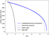 |
Fig. 1 Time evolution of the pebble cloud size in the non-linear numerical simulation, a static gas solution (Eq. (1)), and the analytical solution (solution 2) in the terminal velocity approximation (shown with solid, dashed, and dotted lines, respectively). The black line corresponds to the standard freefall, without friction (see Appendix A.1). |
2.2 Governing equations
The gas dynamics is described by the inviscid Euler equations:
 (4)
(4)
 (5)
(5)
 (6)
(6)
where ρg , u, P, and E are respectively the mass density, the velocity, the pressure, and the total energy (kinetic and internal) of the gas. We studied the self-gravity of the gas and dust, and the drag force between them. In the momentum equation, ρp is the local pebble mass density. The equation system is closed with an ideal equation of states written as
 (7)
(7)
where R, M, T, U, and γ are the ideal gas constant, the molar mass, the temperature, the internal energy and the adiabatic index of the gas.
Pebbles are modelled as a pressure-less fluid whose dynamic is described as
 (8)
(8)
 (9)
(9)
where ρd and vd are the mass density and the velocity of the fluid. ϕg+p is the gravitational potential of both gas and pebbles, which solves the Poisson equation
 (10)
(10)
where ρg+p is the total mass density of gas and pebbles. ϕc is addressed in Sect. 3 where its introduction is justified by the limited simulation domain.
In these equations, adrag is the drag acceleration exerted by the gas on pebbles (and −adrag the feedback onto the gas). The drag acceleration is computed with the prescription
 (11)
(11)
where τs is the dust stopping time given by
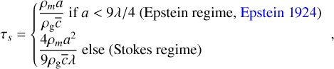 (12)
(12)
depending on the material density ρm and size a of the pebbles, the density ρg of the gas and the mean thermal speed of the gas molecules  , with cs the sound speed in the gas. λ is the mean-free path of the gas molecules. In the energy equation, 𝒫drag is the power given by the particles to the gas, defined as
 (13)
(13)
This includes the power imparted by the drag force and the frictional heating, which can be considered as irreversible power generating entropy.
Finally, in the collapsing area, the pebbles are highly concentrated compared to the disc mean solid density. We treated this area as being composed of regions with a large concentration of dust of many sizes (not included in the simulations) and therefore optically thick. We then considered an adiabatic evolution for the system of gas and pebbles.
2.3 Static gas
An estimation of the heating by gravitational collapse could be provided assuming here a static gas and using an energetic approach where the initial gravitational energy of the pebbles would be fully converted into gas internal energy. This would mean that the pebbles fully transfer their kinetic energy to gas through friction. This simple approach mimics some estimations made to obtain an upper limit on the temperature of a geophysical body (see e.g. Lichtenberg et al. 2023, Sect. 2.1.1).
The initial condition is a spherical pebble cloud with a uniform mass density1. The gravitational energy of the ball of mass M and initial radius R0 is  . An infinitesimal contraction of the pebble ball releases the gravitational energy,
 (14)
(14)
Assuming this released gravitational energy spread uniformly in the ball of the same radius R, the gas temperature would increase by this infinitesimal contraction by
 (15)
(15)
with cv the molar heat capacity at constant volume and Vm the molar volume. The gas shell of radius  receive energy from the solids through drag only when the pebble cloud is larger than
  . The temperature at a radius
  would have increased by the end of the collapse of
 (16)
(16)
For a pebble cloud of mass 3 × 10¹⁶ kg contracting from R0 = 1500 km to  km, the gravitational energy released is
  J. If this energy is deposited through the process described above in a gas initially at 320 K and 8.34 Pa composed fully of H2, (which corresponds to a total mass of about 9 × 10¹³ kg, and cv = 20.8 J⋅mol−1⋅K−1) the temperature would reach more than 5000 K according to Eq. (16).
This simple approach gives an upper limit to gas heating. The very high temperature obtained here shows that the hypothesis of a full conversion of gravitational energy into gas internal energy is not correct. Therefore, a more complete approach, including the gas and dust thermal as well as dynamical evolution with fully non-linear numerical simulations is necessary.
Range of values used for our runs.
3 Numerical methods
We performed 1D spherically symmetric simulations using the IDEFIX code (Lesur et al. 2023b), solving the hydrodynamical equations with finite-volume methods through a Godunov scheme. IDEFIX also includes a self-gravity module (see Appendix A of Mauxion et al. 2024) to solve the Poisson equation with linear algebra methods. The solids can be modelled in two ways. In this study we chose to model them as a pressure-less fluid. We provide a comparison with a Lagrangian particle model in Appendix C, showing that for our problem the two approaches are similar. The runs have been performed using a second-order Runge–Kutta scheme, second-order spatial reconstruction and the Lax–Friedrichs Riemann solver.
3.1 Initial conditions
Initially, the pebbles were static, forming a clump with a uniform density profile in the core and a Gaussian tail at the edge:
 (17)
(17)
Here rc is the initial core radius of the clump, and we defined the initial radius of the pebble sphere as R0 = rc + σ with σ = rc /5. The gas had no initial velocity, a uniform density ρ0 and temperature T𝑔 with an ideal equation of state. The adiabatic index of the gas was 1.4. The initial stopping time τp was 8.4 × 10⁴ s corresponding (for the chosen gas density and sound speed) to pebbles with a = 15 cm and ρm = 3 g⋅cm−3 , and to Stff = 0.06. For these pebbles, the stopping time was computed in the Stokes regime.
Our fiducial simulation had a pebble mass Mfid of 3 × 10¹⁶ kg and gas density ρfid of 7 × 10⁻⁶ kg⋅m−3. This fiducial mass corresponded to a core density ρc of 2.1 × 10⁻³ kg⋅m−3 in Eq. (17), and thus to an initial dust-to-gas ratio of 300. We explored how changes in the total pebble mass, Mtot, and initial gas density, ρ𝑔, affect the final temperature. The values employed for the various runs are presented in Table 1. Assuming a planetesimal density of 2000 kg⋅m−3 (which would correspond to planetesimals made of silicates with some porosity), these initial masses correspond to spherical planetesimals with radii between 10.6 and 26.1 km. The initial size and mass of our pebble cloud are therefore small compared to the characteristic size of the parent bodies of the current main belt asteroids. The initial gas temperature (320 K) corresponds to the inner region of a solar-type star protoplanetary disc. The initial pebble clump radius R0 is 1500 km (that is rc = 1250 km and σ = 250 km).
3.2 Grid and resolution
We performed 1D spherically symmetric simulations with a grid extending from Rin = 0.0013R0 to Rout = 4R0 or equivalently [2, 6000] km. The grid was uniform from 2 to 30 km and logarithmic from 30 to 6000 km giving a good balance between precision and numerical time. A grid comprising 2048 cells was considered, of which 306 are located in the uniform part from 2 to 30 km resulting in cells of 90 m. In the logarithmic part, the ratio between the grid spacing and position ∆x/x is approximately 0.003. This distribution of cells was designed such that the cell size in the uniform zone is comparable to the size of the first cell in the logarithmic zone. To circumvent the singularity at the centre and the considerable computational expense, the central zone between 0 and 2 km was not included in the simulation. Nevertheless, the mass of the gas and particles situated within this zone was represented by a central point mass, with the gravitational potential (ϕc) incorporated into the self-gravity potential in Eqs. (5), (6), and (9).
3.3 Boundary conditions
At the outer edge, the outflow boundary condition is used with extrapolated primitive quantities. We performed tests with different boundary conditions and no apparent difference has been seen with zero gradient boundary conditions, showing that the size of the grid was chosen large enough to avoid such numerical artefacts.
At the inner edge, we used a no-inflow boundary condition. The density and pressure (for the gas) were copied from the innermost cell to the ghost zone (no gradient), the radial velocity was capped at 0 in ghost cells, and the mass flux was set to 0 if a positive flux is entering the simulation grid. The mass lost at the inner edge was appended to the central point mass, thereby contributing to the overall dynamics of the system via the potential ϕc .
3.4 Test
To test the code and verify the compatibility of the different modules, we reproduced the results obtained by Shariff & Cuzzi (2015). The main difference in the approach is the numerical methods used to solve the hydrodynamic equations, and the boundary condition at the inner edge of the grid. Our approach shows good agreement with their results (as presented in Appendix B.1), proving that we have correctly captured the physics.
4 Numerical results of gravitational collapses
4.1 Fiducial run
Figure 2 shows radial profiles of the particle density and the evolution of the central gas density and temperature of our fiducial run. This reference run done with the Eulerian approach for the pebbles has a freefall time of tff = 1.44 × 10⁶ s. The mean radius evolves from 0.5R0 at the beginning of the simulation to 0.02R0. This final mean radius corresponds to a core radius of 100 km. The collision time starts to be smaller than the friction time (see Appendix A.2 for estimation of these times). The collisions not being included here, we did not follow the collapse further. The temperature plotted here (dashed red curves) is computed from the primitive variables, density (dotted green curves) and pressure, using the perfect gas law.
The radial density profile of the pebble cloud is shown on the left of Fig. 2. The core of the cloud has a radially uniform density for most of the collapse but the concavity of the tail changes and the edge of the cloud becomes steep. Its value increases with time during the collapse, to reach 30 kg⋅m−3. However, this increase is not regular in time. The initial density is multiplied by 100 before 4.7 tff, and then multiplied by another factor of 300 at the end of the run, only 0.1 tff later. We find the same behaviour for the gas density and temperature (shown on the right). They are almost constant during the collapse up to 4.7 tff (i.e. (tcol − t)/tff ~ 10−1) and change only at the end of the collapse, with a final increase in the central density by a factor of 3 and of the gas central temperature by about 170 K. It can be seen that the temperature evolution occurs only within the pebble cloud. In particular, the edge of the temperature rise zone and the edge of the pebble cloud overlap quite well. The increase in gas temperature of 170 K, small compared to the value estimated in Sect. 2.3, also shows that the simple approach used there is not correct, as it assumes the pebble kinetic energy to be fully converted into gas heating. In fact, the kinetic energy represents indeed more than half of the released gravitational energy.
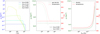 |
Fig. 2 Evolution of the cloud during the collapse. Left: time evolution of the radial profile of the particle cloud density. Centre: gas temperature profiles (dashed red) and gas density profiles (dotted green), plotted at the beginning and the end of the fiducial run. Right: time evolution of the central density (dotted green) and temperature (dashed red, right axis) of the gas. |
4.2 Heating processes
This section examines the heating that occurs during the fiducial run. Initially, the gas is a reservoir of gravitational energy with no kinetic energy, with two external sources of energy: the frictional heating of particles depositing their gravitational energy in the gas, and an energy transfer at the domain outer boundary. The latter would result in a temperature increase also at the outer edge of the computational domain, which we do not see. The central heating is not an outer boundary effect. Therefore, to identify the origin of the gas heating in the fiducial run, we followed Huang & Bai (2022) and introduced a gas frictional heating parameter, ω, to Eq. (13):
 (18)
(18)
The ω parameter ranges from 0 for no frictional heating of the gas (in other words this energy would heat the particles) to ω = 1 corresponding to a full transfer of the energy dissipated through friction to gas thermal energy. We compare in Fig. 3 the evolution of the central gas temperature during the contraction for two extreme cases ω = 1 and ω = 10−3. The weak difference indicates that frictional heating is negligible compared to compressional heating, with a contribution of 1 K to the total temperature increase of about 170 K, as shown by the inset in Fig. 3. As it will be discussed subsequently, this variation is of a similar magnitude to that introduced by modifying the resolution of our grid. Therefore, this is not a physically significant phenomenon. This shows that the heating of the gas is not due to the irreversible term of Eq. (13). We also note that the density minimum seen in Fig. 2 is not present for weak frictional heating.
We next considered particle drag as a precursory process initiating the gas compression responsible for the temperature increase. We compared the gas temperature with the adiabatic evolution given by the Laplace law for perfect gas (dashed curve in Fig. 3). The two curves perfectly overlap, showing that adiabatic heating is the main process responsible for the gas temperature increase at the centre of the cloud. To identify how the adiabatic compression occurs, we show in Fig. 4 the radial profiles computed for the two extreme values of ω at the same run time. One can see that the density radial profiles (blue), and the central and outer temperature (red) perfectly match in the two runs. This is consistent with the irreversible term being negligible in the collapse dynamics. A temperature mismatch is seen only at the cloud rim that coincides with the region of non-negligible frictional heating (ω = 1). The irreversible term of Eq. (13) has a non-negligible contribution only at the edge of the pebbles cloud. In this region, the temperature increase is higher for ω = 1 than ω = 0.001. Finally, the amplitude of the (negative) drag force that does not vary with ω, is maximum also at the cloud rim. Indeed, most of the pebbles’ momentum is at the cloud edge, so this layer dominates the work of the drag force transferred to the gas. Furthermore, one can see that the gas pressure gradient and the drag force are nearly opposite. Consequently, the pebble drag action on the gas can be conceptualised as a piston compressing and heating the inner gas in an adiabatic process.
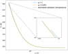 |
Fig. 3 Gas central temperature as a function of the cloud mean radius for two extreme values of ω. The dotted curve corresponds to the theoretical temperature for an adiabatic evolution. |
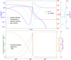 |
Fig. 4 Radial profiles of the pebble density, gas temperature, pebble velocity, and gas velocity (top) and the frictional heating, drag force, and gas pressure gradient (bottom) at t/tff = 4.756 for ω = 1 (the fiducial case) and ω = 0.001. |
4.3 Thermal exchanges between gas and pebbles
In this section we consider the thermal exchanges between the gas and the pebbles that were previously neglected. To include these thermal exchanges, we now also consider the time evolution of the specific internal energy of the pebbles ud. It is advected with the flow of pebbles with velocity υd and is calculated as:
 (19)
(19)
Here Sd is the source term modelling representing the thermal energy transfer from the gas to the pebbles. It is therefore subtracted from the gas energy equation to ensure the energy conservation of the whole system.
A rigorous estimation of these thermal exchanges is complex and would require a precise understanding of the structure of the pebbles (size, shape, composition, porosity, etc.). With Sd representing heat transfer at the surface of spherical pebbles, we can write (see e.g. Bird et al. 2006, Eq. (14.1.1))
 (20)
(20)
In this equation, h is the heat transfer coefficient associated with the fluid and s is the exchange surface between gas and pebbles per fluid volume. h is computed from the gas thermal conductivity k (given by the kinetic theory of gases) and the size of pebbles a through the Nusselt number  . We used the expression of the Nusselt number given by Bird et al. (2006, Eq. (14.4.5)) Nu = 2 + 0.6Re1/2Pr1/3. For the flow considered in our simulation of a perfect gas around pebbles, we have Re ≪ 1 and Pr ~ 1, so we considered Nu ≈ 2 and therefore
  . Moreover, s is given by
  , where the first term is the number density of pebbles and the second the surface of a pebble. Finally, T𝑔 is the gas temperature and Td is the temperature of the pebbles. The pebble temperature is related to the internal energy through the specific heat capacity of pebbles Cd. We considered the initial pebble temperature to be at the equilibrium with the gas and defined the internal energy as the variation from the initial one. We therefore have
 (21)
(21)
Three values of Cd (the efficiency of heat transfer through a pebble) were considered:
Cd is the specific heat capacity of silicates CSi (~900 J · kg−1 · K−1). This means that the thermal diffusion inside a pebble is very efficient, and the temperature is uniform throughout the solid.
Cd = 0.01 CSi: thermal diffusion is weakly efficient on timescales involved here and only 1% of pebbles heat.
Cd = 0.001 CSi: thermal diffusion is poorly efficient and only the very surface of pebbles heats.
We also note that Cd = 0 corresponds to our previous simulations (no heating of the pebbles). With this approach, the resulting surface temperature of the pebbles is very similar to the gas one. The increase in gas temperature at the inner edge of the simulation varies strongly with the specific heat capacity, as shown in Table 2. This is an expected result as the energy converted from the pebble velocity to internal energy is distributed into the gas and a mass of solids, and this mass varies significantly. At the end of the simulation, way before the end of the collapse, the pebble-to-gas ratio is already very high (of the order of 105–106, as can be seen in Fig. 2), and the internal energy lies mostly in the pebbles.
This result raises questions regarding how the total amount of internal energy that will be distributed between gas and solids varies with the properties of the initial cloud. The thermal diffusion properties of the pebbles being unknown, we consider in the following this global internal energy of the system as represented by the gas temperature when the pebbles do not heat (Cd = 0).
4.4 Parameter exploration
4.4.1 Initial mass and density
We studied how the final central gas temperature evolves with two parameters: the total mass of the pebble cloud, Mtot, and the initial gas density, ρ𝑔, characterised as Mfid = 3 × 10¹⁶ kg and ρfid = 7 × 10⁻⁶ kg · m−3. As shown in Fig. 5, the final central temperature is approximately inversely proportional to the square root of the initial gas density. However, the slope of the curve varies slightly with the initial cloud mass. To better characterise this behaviour, the final temperature is plotted as a function of the initial mass in Fig. 6. The final temperature is nearly proportional to the initial mass, but again, with a slight dependence on the gas density.
These behaviours are consistent with what we might expect: the more massive the pebble clump, the more energy is released, and the higher the temperature of the gas surrounding the forming planetesimal. Similarly, if there is less gas surrounding the clump, the gas will be hotter, for the same amount of energy released. These results show that, to dissolve gas from the disc into the forming planetesimal (i.e. to reach a temperature of about 1200 K), a massive clump (mass of about 1017 kg, corresponding to a planetesimal of about 20 km in size) with a low surrounding gas density (initial dust-to-gas ratio of about 1000 or more) is required, as well as a nearly zero thermal diffusion in the pebbles.
Gas temperature increase as a function of the strength of thermal exchanges between gas and pebbles.
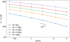 |
Fig. 5 Increase in the gas central temperature as a function of the initial gas density for different values of the initial mass of pebbles. |
4.4.2 Size and intrinsic density of pebbles
We also studied the influence of the coupling between gas and particle by varying the initial stopping time of the pebbles. This was done by modifying either the size or the internal density of the pebbles. Sizes between 5 and 20 cm and densities between 1 and 7 g · cm−3 were chosen (pebbles made of different materials from ice to iron depending on porosity). Because of the transition in the formulation of the stopping time between the Epstein and Stokes drag law for s = 6.9 cm in our fiducial setup where the mean free path of the gas is λ = 2.9 cm, there is a dichotomy in behaviour between the 5 cm pebbles and the others. For solids larger than 10 cm, one can see in Fig. 7 that the smaller the initial stopping time, the hotter the gas at the end of the run. The drag term in Eqs. (5) and (6) is inversely proportional to the stopping time. Thus, for smaller and less dense pebbles, more coupled to the gas, the piston effect is more efficient and the gas temperature is higher. This correlation between the stopping time and adiabatic heating is also responsible for the dichotomy seen in Fig. 7 between the 5cm size pebbles and the other, for the same initial stopping time. Indeed in a perfect gas, the mean free path λ is proportional to  . Therefore, with Eq. (12), we have
  for Epstein law and
  for Stokes law. It implies that for a fixed-size solid the modification of its stopping time with the gas density and temperature is larger in the Epstein regime. Thus, for two pebbles with the same initial stopping time, the one in the Epstein regime will become more coupled to the gas as the collapse progresses than the one in the Stokes regime. So, at the end of the simulation, the piston effect will be more efficient for small pebbles than for big ones.
Figures 5, 6, and 7 demonstrate that the maximum temperature increase in the gas is achieved when the initial gas density is the lowest, the total mass of the cloud is the largest or the pebbles are the smallest. In the parameter range under consideration (see Table 1), the greatest temperature increase is therefore observed for Mtot = 5Mfid, ρ𝑔 = 0.5ρfid and a = 5 cm. We ran the corresponding simulations and show the results as the black dots in Fig. 7. In this case, we obtain an increase of about 1300 K resulting in a final temperature of approximately 1600 K.
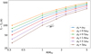 |
Fig. 6 Increase in the gas central temperature as a function of the initial mass of pebbles for different values of initial gas density. |
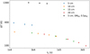 |
Fig. 7 Gas central temperature increase as a function of the initial stopping time of pebbles. |
5 Discussion and conclusion
To ascertain the impact of numerical resolution on our results, additional simulations were conducted using the same initial conditions as the fiducial case but with an increasing number of cells. The findings are presented in Appendix B.2. We verified that increasing the resolution does not change the physical results, whereas decreasing it could occasionally result in minor numerical instabilities.
Our initial exploration of the parameter space highlights the importance of the gas heating process during planetesimal formation via gravitational collapse. However, due to the simplicity of our approach, there are several limitations.
First, the collapse is assumed to be spherically symmetric. This implies that convection in the gas and rotation are neglected. In our fiducial simulation, we estimated the Brunt–Väisälä frequency (N), finding the value of N2 to be positive in the edge zone at a radius r ≈ 105 km. However, the value of N is ≈ 10−4 Hz, resulting in a characteristic time of 104 s. This timescale is of the order of the temperature evolution timescale, casting doubts on the viability of genuine convection. So, the temperature profiles shown in Fig. 2 reached at the end of the simulation might be prone to convection. However, this estimation was made without taking cooling into account. Including cooling would lead to a redistribution of energy within the gas, which would reduce the final central temperature.
Finally, we did not consider particle collisions, despite their potentially key role in planetesimal formation (Nesvorný et al. 2010, 2021; Wahlberg Jansson et al. 2017; Wahlberg Jansson & Johansen 2017; Polak & Klahr 2023), for two reasons. First, we ran 1D simulations with no initial velocity dispersion, making collisions meaningless here. Second, unlike Nesvorný et al. (2010, 2021), who focused on Kuiper Belt objects, we considered planetesimal formation closer to 1 AU with denser and hotter gas, which leads to stronger friction that can dominate the effect of collisions in the first phase of the collapse (see a comparison between stopping time and collision time in Appendix A.2). It is a reasonable assumption that collisions will play a crucial role in the subsequent evolution. This is due to the fact that collisions will facilitate a conversion of the kinetic energy of the pebbles into internal energy, which will in turn influence the temperature of the pebbles.
To conclude, in this study we have extended the Shariff & Cuzzi (2015) modelling of the gravitational collapse of a gas and pebble cloud by considering the gas thermodynamics. We first see an increase in the collapse time of the pebble cloud due to the gas friction. This increase is inversely proportional to the Stokes number, Stff = 2πτs/tff. Secondly, we have provided evidence that the heating of the gas at the centre of the domain is caused by gas adiabatic compression driven by the pebbles dragging the gas with them as they collapse. We identify three regions that are associated with different heating. In the outermost region without particles, there is no temperature increase. Frictional heating, when present, heats only the particle cloud rim. The temperature rise in the core of the cloud is dominated by adiabatic compression driven by the deposition of momentum in the rim. We also show how this heating varies with the clump mass, the gas density, and the characteristics of the pebbles. In the most massive clumps, more gravitational energy will be released during the collapse, and thus the pebbles will reach a higher velocity. Moreover, if these clumps are made of small pebbles, the coupling between pebbles and gas is stronger, which implies that the piston effect is more efficient. Therefore, in these clumps, the gas might reach the temperature needed for dissolution into the forming planetesimal.
The final stages of the collapse were not modelled in this study. If these stages were simulated, a higher temperature would likely be reached. The temperature might be high enough (up to about 1500 K) for the pebbles to experience thermal meta-morphism and perhaps even melt, allowing gas to dissolve into them or leading to a release of trapped gases. However, this would strongly depend on the extent of the thermal exchanges between gas and pebbles and on their compositions. At such pebble scales, geochemical experiments of gas dissolution into silicates show that this process could be highly effective in a few hours (see e.g. Jambon et al. 1986). Our work demonstrates that the pebble surface could melt during the gravitational collapse over a timescale of 10−2 freefall times (5 hours here) in favourable conditions (a massive clump, small pebbles, and low to near-zero thermal diffusion). Therefore, even for planetesi-mals that are small compared to the characteristic size of the parent bodies of the current main belt asteroids, the temperature increase might be consistent with gas dissolution in the planetesimal-forming pebbles. However, one should note that the cooling process after the planetesimal formation was not taken into consideration in this study.
These results emphasise the key role of gas in the formation of planetesimals via gravitational collapse, especially at distances of a few AUs from the central star. This implies a new step in the thermal history of planetesimals that depends strongly on their formation region. The identified heating process may lead to local heating not only in space but also in time, which could provide new approaches for cosmochemical studies. This work also suggests future avenues for studying the gravitational collapse of a pebble clump in a gaseous environment: first, by extending the simulations to 2D or 3D, opening up the possibility of including initial particle velocity dispersion and collisions, and second, by better modelling the thermal exchange between pebbles and gas.
Acknowledgements
This work was supported by the French government through the France 2030 investment plan managed by the National Research Agency (ANR), as part of the Initiative of Excellence Université Côte d’Azur under reference number ANR-15-IDEX-01. The authors are grateful to the Université Côte d’Azur’s Center for High-Performance Computing (OPAL infrastructure) for providing resources and support. It has received support from the CNRS Origines and ‘Programme national de Planétologie’ (PNP). The authors would like to thank the anonymous referee for the very useful comments that helped to improve greatly this paper.
Appendix A Derivation of analytic formulas
A.1 Freefall time
The freefall time of a particle clump can be calculated using the same reasoning as in Sect. 2.1. The position of a freefalling particle at the cloud edge is calculated as
 (A.1)
(A.1)
This equation can be integrated for a static initial condition and an initial radius, R0, becoming
 (A.2)
(A.2)
 (A.3)
(A.3)
where x = r/R0. The freefall time corresponds to the time when r (or x) reaches 0:
 (A.4)
(A.4)
A.2 Collision time versus stopping time
Building on Nesvorný et al. (2010), we compared the stopping time and the time between pebble collisions. The stopping time was estimated in the Epstein regime as  . The collision time is given by τc ~ (ոσυ)−1 , with the pebbles number density n ~ Mtot/(ρma3R3), the cross-section σ ~ a2, and the virial velocity
  . Bringing all together leads to
 (A.5)
(A.5)
With the values for  , and R used in our fiducial simulation, we have τs/τc ~ 1. Thus, the stopping time and the collapse time are approximately the same in this situation and thus the friction due to the gas cannot be neglected. However, we have here υ ~ 1 m · s−1, which is an order of magnitude higher than the typical velocity observed in our simulation (a so high velocity is obtained only at the end of the collapse). We can then consider that for our simulations, τs ≪ τc, and so the friction is dominant for most of the collapse period.
Appendix B Test of the numerical setup
B.1 Comparison with previous work
To test our numerical setup, we compared it with the work of Shariff & Cuzzi (2015), who used a similar approach for the modellisation of the system but with different numerical methods for solving hydrodynamics and Poisson equations. Moreover, we tested the Lagrangian particle module of IDEFIX, which solves the dynamics of the pebbles very differently
The notations used here are the same as in Sect. 4.1 of Shariff & Cuzzi (2015). The Jt corresponds to a two-phase Jeans number and compares the propagation time of a sound wave across the clump with the dynamical time  .
.
 |
Fig. B.1 Size evolution of the particle cloud for various Jt (Stff = 0.02. ϕ0 = 100) with our Eulerian approach for pebbles. |
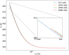 |
Fig. B.2 Evolution of the gas central temperature with the cloud mean radius for different numerical refinements. |
Figure B.1 compares the size evolution of the clump for various Jt and should be compared with Fig. 3 of Shariff & Cuzzi (2015). We obtain results similar to those of the original study, which validates our methodological approach.
B.2 Convergence test
We ran our fiducial run for different resolutions, from 512 to 4096 cells. The results are shown in Figs. B.2 and B.3. We see that increasing the resolution does not change the physical results (small variation of about 2 K, which is 1% of the temperature increase at the end of the collapse). However, we see that at low resolution there are some numerical instabilities at the edge of the cloud. We therefore decided to use a resolution of 2048 cells as a compromise between these instabilities and the simulation time.
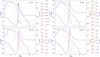 |
Fig. B.3 Radial profiles of pebble density (blue), gas density (green), gas temperature (red), and gas velocity (indigo) at the end of the fiducial simulation (t/tff = 4.756) for different numerical refinements. |
Appendix C Laցranցian particle approach
Two principal methods are typically employed to model the dynamical evolution of solids in gaseous proto-planetary discs. The first is the pressure-less fluid model, which is the focus of this paper. The second method is the Lagrangian particle approach, which involves the modelling of solids through a relatively small number of particles, referred to as super-particles (SPs). Each SP represents a large number of pebbles sharing the same properties, including size, internal density, velocity. The IDEFIX code enables the utilisation of these two approaches, and thus a comparison was undertaken. The principal characteristics of the Lagrangian particles module of the IDEFIX code are presented here, with a more comprehensive account to follow in a dedicated publication.
The SPs follow the Newton equation:
 (C.1)
(C.1)
where xp and υp are the position and the velocity of a SP. In order to compute the self-gravity and friction forces, the deposition of SPs on the grid is carried out using a triangular shape cloud scheme, as described by Mignone et al. (2018).
The simulation of the collapse employs the identical initial conditions and grid as the pressure-less fluid approach, with a single minor alteration. To reduce the computational time, an evolving mesh refinement is implemented. The simulation is conducted in three stages, corresponding to the intervals [0.5, 0.15]R0, [0.15, 0.05]R0, and [0.05, 0.02]R0. At each restart, the resolution is increased from 1024 to 2048 and 4096 cells. This results in a reduction in the requirement for computational resources during the initial phase of the evolution process, while simultaneously enabling high precision during the accelerated evolution phase at the late stages of the collapse. In order to ensure continuity in cell size between the uniform zone and the logarithmic zone of the grid, the cells are distributed between the two zones in the same way as the simulations conducted with the pressure-less fluid approach. To achieve a smooth transition between two different steps, the final profiles from one step were used as the initial conditions for the subsequent step. These profiles, which relate to position, velocity, and pressure (for the gas), are linearly interpolated on the new grid. To obtain sufficient resolution to correctly map the particle density onto the grid, each step was initialised with ten particles per cell. We verified that there were no physical differences if we did only one step with 2048 or 4096 cells. We used open boundary conditions, allowing SPs to escape the grid, thereby precluding any possibility of re-entry. In a manner analogous to the pressure-less approach, the mass lost at the inner boundary is added to the central mass thereby contributing to ϕc.
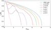 |
Fig. C.1 Size evolution of the particle cloud for various Jt (Stff = 0.02, ϕ0 = 100) with a Lagrangian approach for pebbles. |
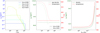 |
Fig. C.2 Evolution of the cloud during the collapse. Left: time evolution of the radial profile of the particle cloud density. Centre: gas temperature profiles (dashed) and gas density profiles (dotted), plotted at the beginning and the end of the fiducial run. Right: time evolution of the central density (dotted) and temperature (dashed, right axis) of the gas. |
Figure C.1 is the same as Fig. B.1, and Fig. C.2 is the same as Fig. 2 but for the Lagrangian particle approach. The results obtained are highly comparable, indicating that both methodological approaches are viable for modelling the collapse. The methodological choice will therefore be contingent upon the additional physical effects one wishes to consider, such as collisions or size distributions.
References
- Bird, R., Stewart, W., & Lightfoot, E. 2006, Transport Phenomena (Wiley) [Google Scholar]
- Blum, J. 2018, Space Sci. Rev., 214, 52 [NASA ADS] [CrossRef] [Google Scholar]
- Boyet, M., Bouvier, A., Frossard, P., et al. 2018, Earth Planet Sci. Lett., 488, 68 [NASA ADS] [CrossRef] [Google Scholar]
- Carrera, D., & Simon, J. B. 2022, ApJ, 933, L10 [NASA ADS] [CrossRef] [Google Scholar]
- Cuzzi, J. N., Hogan, R. C., Paque, J. M., & Dobrovolskis, A. R. 2001, ApJ, 546, 496 [NASA ADS] [CrossRef] [Google Scholar]
- Dittrich, K., Klahr, H., & Johansen, A. 2013, ApJ, 763, 117 [NASA ADS] [CrossRef] [Google Scholar]
- Epstein, P. S. 1924, Phys. Rev., 23, 710 [Google Scholar]
- Fromang, S., & Nelson, R. P. 2006, A&A, 457, 343 [NASA ADS] [CrossRef] [EDP Sciences] [Google Scholar]
- Gerosa, F. A., Méheut, H., & Bec, J. 2023, Eur. Phys. J. Plus, 138, 9 [NASA ADS] [CrossRef] [Google Scholar]
- Gratton, R., Ligi, R., Sissa, E., et al. 2019, A&A, 623, A140 [NASA ADS] [CrossRef] [EDP Sciences] [Google Scholar]
- Hasegawa, Y., Suzuki, T. K., Tanaka, H., Kobayashi, H., & Wada, K. 2021, ApJ, 915, 22 [NASA ADS] [CrossRef] [Google Scholar]
- Hasegawa, Y., Suzuki, T. K., Tanaka, H., Kobayashi, H., & Wada, K. 2023, ApJ, 944, 38 [NASA ADS] [CrossRef] [Google Scholar]
- Hayashi, C. 1981, Prog. Theor. Phys. Supp., 70, 35 [CrossRef] [Google Scholar]
- Huang, P., & Bai, X.-N. 2022, ApJS, 262, 11 [NASA ADS] [CrossRef] [Google Scholar]
- Jambon, A., Weber, H., & Braun, O. 1986, Geochim. Cosmochim. Acta, 50, 401 [NASA ADS] [CrossRef] [Google Scholar]
- Johansen, A., Klahr, H., & Henning, T. 2011, A&A, 529, A62 [NASA ADS] [CrossRef] [EDP Sciences] [Google Scholar]
- Johansen, A., & Lambrechts, M. 2017, Annu. Rev. Earth Planet. Sci., 45, 359 [Google Scholar]
- Keppler, M., Benisty, M., Müller, A., et al. 2018, A&A, 617, A44 [NASA ADS] [CrossRef] [EDP Sciences] [Google Scholar]
- Klahr, H., & Hubbard, A. 2014, ApJ, 788, 21 [Google Scholar]
- Kobayashi, H., & Tanaka, H. 2021, ApJ, 922, 16 [NASA ADS] [CrossRef] [Google Scholar]
- Kobayashi, H., & Tanaka, H. 2023, ApJ, 954, 158 [NASA ADS] [CrossRef] [Google Scholar]
- Krapp, L., Benítez-Llambay, P., Gressel, O., & Pessah, M. E. 2019, ApJ, 878, L30 [Google Scholar]
- Kruijer, T. S., Touboul, M., Fischer-Gödde, M., et al. 2014, Science, 344, 1150 [NASA ADS] [CrossRef] [Google Scholar]
- Lesur, G., Flock, M., Ercolano, B., et al. 2023a, in Astronomical Society of the Pacific Conference Series, 534, Protostars and Planets VII, eds. S. Inutsuka, Y. Aikawa, T. Muto, K. Tomida, & M. Tamura, 465 [NASA ADS] [Google Scholar]
- Lesur, G. R. J., Baghdadi, S., Wafflard-Fernandez, G., et al. 2023b, A&A, 677, A9 [NASA ADS] [CrossRef] [EDP Sciences] [Google Scholar]
- Lichtenberg, T., Schaefer, L. K., Nakajima, M., & Fischer, R. A. 2023, in Astronomical Society of the Pacific Conference Series, 534, Protostars and Planets VII, eds. S. Inutsuka, Y. Aikawa, T. Muto, K. Tomida, & M. Tamura, 907 [NASA ADS] [Google Scholar]
- Lorek, S., & Johansen, A. 2024, A&A, 683, A38 [NASA ADS] [CrossRef] [EDP Sciences] [Google Scholar]
- Lovelace, R. V. E., Li, H., Colgate, S. A., & Nelson, A. F. 1999, ApJ, 513, 805 [NASA ADS] [CrossRef] [Google Scholar]
- Lyra, W. 2014, ApJ, 789, 77 [Google Scholar]
- Manger, N., & Klahr, H. 2018, MNRAS, 480, 2125 [NASA ADS] [CrossRef] [Google Scholar]
- Mauxion, J., Lesur, G., & Maret, S. 2024, A&A, 686, A253 [NASA ADS] [CrossRef] [EDP Sciences] [Google Scholar]
- Meheut, H., Meliani, Z., Varniere, P., & Benz, W. 2012, A&A, 545, A134 [NASA ADS] [CrossRef] [EDP Sciences] [Google Scholar]
- Mignone, A., Bodo, G., Vaidya, B., & Mattia, G. 2018, ApJ, 859, 13 [CrossRef] [Google Scholar]
- Morbidelli, A., & Nesvorný, D. 2020, in The Trans-Neptunian Solar System, eds. D. Prialnik, M. A. Barucci, & L. A. Young (Elsevier), 25 [CrossRef] [Google Scholar]
- Nelson, R. P., Gressel, O., & Umurhan, O. M. 2013, MNRAS, 435, 2610 [Google Scholar]
- Nesvorný, D., Youdin, A. N., & Richardson, D. C. 2010, AJ, 140, 785 [Google Scholar]
- Nesvorný, D., Li, R., Simon, J. B., et al. 2021, Planet. Sci. J., 2, 27 [CrossRef] [Google Scholar]
- Pan, L., Padoan, P., Scalo, J., Kritsuk, A. G., & Norman, M. L. 2011, ApJ, 740, 6 [Google Scholar]
- Polak, B., & Klahr, H. 2023, ApJ, 943, 125 [NASA ADS] [CrossRef] [Google Scholar]
- Raettig, N., Lyra, W., & Klahr, H. 2021, ApJ, 913, 92 [NASA ADS] [CrossRef] [Google Scholar]
- Schaffer, N., Johansen, A., & Lambrechts, M. 2021, A&A, 653, A14 [NASA ADS] [CrossRef] [EDP Sciences] [Google Scholar]
- Shariff, K., & Cuzzi, J. N. 2015, ApJ, 805, 42 [NASA ADS] [CrossRef] [Google Scholar]
- Urpin, V., & Brandenburg, A. 1998, MNRAS, 294, 399 [Google Scholar]
- Wahlberg Jansson, K., & Johansen, A. 2017, MNRAS, 469, S149 [Google Scholar]
- Wahlberg Jansson, K., Johansen, A., Syed, M. B., & Blum, J. 2017, ApJ, 835, 109 [NASA ADS] [CrossRef] [Google Scholar]
- Weidenschilling, S. J. 1977, MNRAS, 180, 57 [Google Scholar]
- Youdin, A. N., & Goodman, J. 2005, ApJ, 620, 459 [Google Scholar]
- Zhu, K., Schiller, M., Moynier, F., et al. 2023, Geochim. Cosmochim. Acta, 342, 156 [CrossRef] [Google Scholar]
We define here a ball as a filled sphere or a solid sphere, and a sphere as the surface of a ball.
All Tables
Gas temperature increase as a function of the strength of thermal exchanges between gas and pebbles.
All Figures
|
Fig. 1 Time evolution of the pebble cloud size in the non-linear numerical simulation, a static gas solution (Eq. (1)), and the analytical solution (solution 2) in the terminal velocity approximation (shown with solid, dashed, and dotted lines, respectively). The black line corresponds to the standard freefall, without friction (see Appendix A.1). |
| In the text | |
|
Fig. 2 Evolution of the cloud during the collapse. Left: time evolution of the radial profile of the particle cloud density. Centre: gas temperature profiles (dashed red) and gas density profiles (dotted green), plotted at the beginning and the end of the fiducial run. Right: time evolution of the central density (dotted green) and temperature (dashed red, right axis) of the gas. |
| In the text | |
|
Fig. 3 Gas central temperature as a function of the cloud mean radius for two extreme values of ω. The dotted curve corresponds to the theoretical temperature for an adiabatic evolution. |
| In the text | |
|
Fig. 4 Radial profiles of the pebble density, gas temperature, pebble velocity, and gas velocity (top) and the frictional heating, drag force, and gas pressure gradient (bottom) at t/tff = 4.756 for ω = 1 (the fiducial case) and ω = 0.001. |
| In the text | |
|
Fig. 5 Increase in the gas central temperature as a function of the initial gas density for different values of the initial mass of pebbles. |
| In the text | |
|
Fig. 6 Increase in the gas central temperature as a function of the initial mass of pebbles for different values of initial gas density. |
| In the text | |
|
Fig. 7 Gas central temperature increase as a function of the initial stopping time of pebbles. |
| In the text | |
|
Fig. B.1 Size evolution of the particle cloud for various Jt (Stff = 0.02. ϕ0 = 100) with our Eulerian approach for pebbles. |
| In the text | |
|
Fig. B.2 Evolution of the gas central temperature with the cloud mean radius for different numerical refinements. |
| In the text | |
|
Fig. B.3 Radial profiles of pebble density (blue), gas density (green), gas temperature (red), and gas velocity (indigo) at the end of the fiducial simulation (t/tff = 4.756) for different numerical refinements. |
| In the text | |
|
Fig. C.1 Size evolution of the particle cloud for various Jt (Stff = 0.02, ϕ0 = 100) with a Lagrangian approach for pebbles. |
| In the text | |
|
Fig. C.2 Evolution of the cloud during the collapse. Left: time evolution of the radial profile of the particle cloud density. Centre: gas temperature profiles (dashed) and gas density profiles (dotted), plotted at the beginning and the end of the fiducial run. Right: time evolution of the central density (dotted) and temperature (dashed, right axis) of the gas. |
| In the text | |
Current usage metrics show cumulative count of Article Views (full-text article views including HTML views, PDF and ePub downloads, according to the available data) and Abstracts Views on Vision4Press platform.
Data correspond to usage on the plateform after 2015. The current usage metrics is available 48-96 hours after online publication and is updated daily on week days.
Initial download of the metrics may take a while.