| Issue |
A&A
Volume 696, April 2025
|
|
|---|---|---|
| Article Number | A245 | |
| Number of page(s) | 17 | |
| Section | Extragalactic astronomy | |
| DOI | https://doi.org/10.1051/0004-6361/202453065 | |
| Published online | 29 April 2025 | |
Polarization flare of 3C 454.3 at millimeter wavelengths seen from decadal polarimetric observations
1
Astronomy and Space Science, University of Science and Technology, 217 Gajeong-ro, Yuseong-gu, Daejeon 34113, Republic of Korea
2
Korea Astronomy and Space Science Institute, 776 Daedeok-daero, Yuseong-gu, Daejeon 34055, Republic of Korea
3
Institute of Astronomy and Astrophysics, Academia Sinica, PO Box 23-141 Taipei 10617, Taiwan
4
Department of Physics and Astronomy, Seoul National University, Gwanak-gu, Seoul 08826, Republic of Korea
5
SNU Astronomy Research Center, Seoul National University, Gwanak-gu, Seoul 08826, Korea
⋆ Corresponding author: This email address is being protected from spambots. You need JavaScript enabled to view it.
Received:
19
November
2024
Accepted:
27
February
2025
Abstract
Context. The blazar 3C 454.3 (z = 0.859) has been extensively investigated using multiwavelength high-resolution polarization studies, showing polarization variations on milliarcsecond scales.
Aims. This study investigates the polarimetric characteristics of the blazar 3C 454.3 at 22–129 GHz using decadal (2011–2022) data sets. In addition, we also delve into the origin of the polarization flare observed in 2019.
Methods. The corresponding data sets were obtained from the single-dish mode observations of the Korean VLBI Network (KVN) and the 43 GHz Very Long Baseline Array (VLBA). Using those data, we compared the consistency of the measurements between milliarcsecond and arcsecond scales. The Faraday rotation measure (RM) values were obtained via two approaches: model fitting to a linear function in all frequency ranges and calculating from adjacent frequency pairs.
Results. We found that the preferred linear polarization angle is ∼100° when the source is highly polarized, for example during a flare. At 43 GHz we found that the polarized emission at of milliarcsecond and arcsecond scales is consistent when we compare its flux density and polarization angle. The ratio of quasi-simultaneously measured (within a week) polarized flux density is 1.02 ± 0.07 (i.e., ΔSp/Sp ≈ 2%) and the polarization angles display similar rotation, which suggest that the extended jet beyond the scale of VLBA 43 GHz has a negligible convolution effect on the polarization angle from the KVN. We found an interesting and notable flaring event in the KVN single-dish data from the polarized emission in 2019 in the frequency range of 22–129 GHz. During the flare, the observed polarization angles (χobs) rotate from ∼150° to ∼100° at all frequencies with a chromatic polarization degree (mp).
Conclusions. Based on the observed mp and χobs, and also on the Faraday rotation measure, we suggest that the polarization flare in 2019 is attributed to the shock–shock interaction in the stationary jet region. The change in the viewing angle of the jet alone is insufficient to describe the increase in brightness temperature, indicating the presence of source intrinsic processes such as particle acceleration.
Key words: polarization / galaxies: active / galaxies: jets / radio continuum: galaxies / quasars: individual: 3C 454.3
© The Authors 2025
 Open Access article, published by EDP Sciences, under the terms of the Creative Commons Attribution License (https://creativecommons.org/licenses/by/4.0), which permits unrestricted use, distribution, and reproduction in any medium, provided the original work is properly cited.
This article is published in open access under the Subscribe to Open model. This email address is being protected from spambots. You need JavaScript enabled to view it. to support open access publication.
1. Introduction
Blazars are a subclass of active galactic nuclei (AGNs) in which a relativistic jet is inclined with a small viewing angle between the jet and the line of sight. The small viewing angle of the jet enhances the Doppler boosting effects, leading to rapid variability. The jet emits radiation over the entire range of electromagnetic waves, which is dominated by synchrotron radiation from radio to optical bands, and radiation by inverse-Compton scattering in higher energy bands (e.g., γ-rays). Synchrotron radiation is emitted by relativistic electrons gyrating around magnetic field lines in the jet.
The synchrotron radiation from the relativistic jets is most likely polarized, with its polarized properties strongly constrained by magnetic field environments in the jet. If the field lines in the jets are well ordered and strong, a high degree of linear polarization (mp) and high polarized flux density (Sp) can be observed. Theoretically, for an ideal case (i.e., a perfectly ordered magnetic field), mp reaching up to ∼75% is feasible for electrons having power-law energy distribution in an optically thin (e.g., α = −1, where S ∝ να) region (Rybicki & Lightman 1979; Trippe 2014). Meanwhile, for an optically thick region, the observed mp is expected to decrease (e.g., by only a few percent of mp).
In addition, observational results have identified polarized emission from AGN, and both mp and the polarization angle (χ) seem to give information about the magnetic field lines in a jet. Several studies have reported the results of polarization observations in both radio and optical bands for AGNs and found highly polarized emission reaching a few tens of percent in polarization degree (Jorstad et al. 2005, 2007; Pushkarev et al. 2023). As the optically thick region is believed to have low mp, even with perfectly ordered magnetic field lines, this implies an optically thin polarized emission from some AGNs at high radio frequency (e.g., ≳86 GHz), since optical wavelengths are optically thin by default. Angelakis et al. (2016) suggested a model discriminating between low- and high-synchrotron peak (LSP and HSP, respectively) blazars based on the optical polarimetry (see also Blinov & Pavlidou 2019). In their work, at optical wavelengths it seems that LSP blazars exhibit highly polarized emission with a random χ distribution and opposite characteristics (i.e., a low degree of polarization with a specific χ) for HSP blazars.
Recently, at shorter wavelengths, the Imaging X-ray Polarimetric Explorer (IXPE) has been observing polarized emission X-rays from celestial objects, including AGNs, and has identified jet models of the AGNs by comparison with radio and optical polarization behavior (Di Gesu et al. 2022; Marinucci et al. 2022; Liodakis et al. 2022; Middei et al. 2023a; Peirson et al. 2023; Middei et al. 2023b; Kim et al. 2024). Among the X-ray studies, the highest measurement in mp is about 22%. However, we note that the polarization degrees listed above are not representative values at each observing frequency since the samples and observing periods are different from each other.
Although the observed polarization angle χobs most likely provides us with information about the orientation of magnetic field lines in the jet, the Faraday effect contaminates the intrinsic polarized emission when the emission propagates through an ionized medium with magnetic field lines (Burn 1966; Sokoloff et al. 1998). This leads to a rotation of χ, which is proportional to the squared wavelength, Δχ ∝ RM λ2, where Δχ = χobs − χ0 (with χ0 is the intrinsic polarization angle). The observed polarization angle can then be written in the form of χobs = χ0 + RM λ2, where χobs is the observed polarization angle and λ is the observing wavelength. RM is the Faraday rotation measure, indicating the amount of rotation in the polarization angle by a medium in units of rad m−2. Therefore, the Faraday rotation is larger at longer wavelengths. Based on this expression, we can calculate the RM as  , where χ1 and χ2 are the observed polarization angles at wavelengths λ1 and λ2, respectively. For a cosmological source at redshift z, RM is defined as
 (1)
(1)
where me and e are the mass and charge of an electron, c is the speed of light, ne is the electron number density of a Faraday screening medium, B∥ is the magnetic field strength along the line of sight, and l is the path length through the medium where the Faraday rotation takes place.
At millimeter wavelengths, the Institute for Radio Astronomy in the Millimeter Range (IRAM) 30 m radio telescope has monitored 37 AGNs at 86 and 229 GHz (Agudo et al. 2018a) in dual-polarization mode to investigate the linear polarization variability of the AGNs (Agudo et al. 2018b). In their work, they found faster variability and larger fractional linear polarization at 229 GHz than at 86 GHz.
The sign of RM depends on B∥ to the line of sight, as indicated in Equation (1). A few multiwavelength polarization studies have revealed high absolute RM (|RM|) values of ∼105 rad m−2 in the observer’s frame (e.g., Kuo et al. 2014; Park et al. 2018; Agudo et al. 2018b; Hovatta et al. 2019). In the Atacama Large Millimeter Array (ALMA) observations, a higher order of |RM| (∼107 rad m−2 in observer frame) was found from a gravitationally lensed AGN called PKS 1830−211 at 250–300 GHz pair (Martí-Vidal et al. 2015). This was attributed to high ne and/or strong B∥ of the screening medium (see Equation (1) in their work).
The blazar 3C 454.3 (z = 0.859) has been extensively investigated in multiwavelength high-resolution polarization studies. In very long baseline interferometry (VLBI) observations at 15 GHz, the source was resolved with a widely extended jet structure beyond ∼10 mas from the central engine, ejecting toward the northwest side (Lister et al. 2018, 2021; Pushkarev et al. 2023). At 43 GHz, two prominent regions have been identified over a decade: the core and a quasi-stationary component (0.45–0.70 mas away from the core, hereafter, Region C, Jorstad et al. 2017; Weaver et al. 2022). Typically, Region C exhibits a higher polarization degree than that of the core with a stable polarization angle aligned to ∼90° (an east-west direction, Kemball et al. 1996; Jorstad et al. 2005, 2013; Traianou et al. 2024). Based on its observed properties, including re-brightening, decrease in the angular size of the jet, and spatial stationariness (Gómez et al. 1999; Jeong et al. 2023), Region C was suggested as a recollimation shock. For a downstream region, Zamaninasab et al. (2013) found a large-scale helical magnetic field structure in 3C 454.3 by comparing the predictions of the helical jet model and observed polarimetric properties across the jet, using the multifrequency Very Long Baseline Array (VLBA1) observations.
Several studies were conducted to evaluate magnetic field strength in the jet of 3C 454.3. Based on the core-shift effect, the magnetic field strengths at the 43 GHz core and 1 pc from the central engine were found to be in 0.03–0.11 G and 0.2–1.13 G, respectively, within 1σ uncertainty (Pushkarev et al. 2012; Kutkin et al. 2014; Mohan et al. 2015; Chamani et al. 2023). In addition, Jeong et al. (2023) estimated magnetic field strengths of the optically thick (τ = 1) surface in the jet via the synchrotron self-absorption (SSA) effect. They found two distinctive SSA components, LSS and HSS (LSS: lower turnover frequency SSA spectrum and HSS: higher turnover frequency SSA spectrum; for more details, see Figure 4 and the text in Jeong et al. 2023), which have turnover frequencies at the low-frequency (≲30 GHz) and high-frequency (≳60 GHz) range. The estimated magnetic field strengths of the HSS were in the range of 0.1–7 mG. The LSS identified before the γ-ray flare in June 2014 (Buson 2014) corresponds to Region C, and they found a magnetic dominance based on a higher SSA magnetic field strength than that in the equipartition condition.
For this study we investigated the decadal polarimetric characteristics of the source using the simultaneous multifrequency (22–129 GHz) single-dish observations from the Korean VLBI Network (KVN2). We also employed the data from the 43 GHz VLBA, managed by the Boston University (BU3) group. The obtained VLBA data were used for comparison with the KVN data at 43 GHz and to resolve the source structure. The data sets used in this study have a time range from 2011–2022, and several γ-ray activities were reported in this period (Buson 2014; Jorstad et al. 2015; Ojha 2016; Panebianco et al. 2022). The observations included in this study will be described in Section 2. The variability of the arcsecond-scale structure observed by the KVN single-dish and the variability of the milliarcsecond-scale structures resolved by the VLBA are shown in Section 3.1. We investigated the Faraday rotation measure using the KVN observations in Section 3.2. In Section 4 we discuss the observed features in the core and Region C. Our conclusions and a summary of this work are presented in Section 5.
2. Observations and data reduction
2.1. The KVN single-dish
MOGABA (MOnitoring of GAmma-ray Bright Active galactic nuclei; Kang et al. 2015) is one of the polarimetric monitoring programs using the KVN on AGNs through the single-dish mode. Another monitoring program, PAGaN (Plasma-physics of Active Galactic Nuclei; Park et al. 2018), has also been conducted for VLBI polarimetry, and their joint single-dish observation is used to calibrate the absolute polarization angle (Kam et al. 2023). 3C 454.3 is one of the target sources of MOGABA and PAGaN.
This work used polarimetric monitoring data in the time periods 2011–2022 (MOGABA) and 2016–2022 (PAGaN) from the KVN 21 m radio telescopes at 22, 43, 86, and 129 GHz on 3C 454.3 in single-dish mode; the corresponding beam sizes are approximately 133, 68, 34 and 23 arcseconds. The KVN consists of three identical 21 m antennas located in Seoul (KVN-Yonsei, KYS), Ulsan (KVN-Ulsan, KUS), and Jeju (KVN-Tamna, KTN); it has a unique capability of simultaneous four-frequency (22, 43, 86, and 129 GHz) observation in VLBI mode. In single-dish mode observation, two antennas were employed quasi-simultaneously (e.g., KTN at 22/43 GHz and KYS at 86/129 GHz). The polarimetric observables are recorded via the circularly polarized feed horns in the KVN receiver.
The polarimetric properties were measured using eight sets of position-switching scans with a bandwidth of 512 MHz after correcting antenna pointing via cross-scan observation. Several unpolarized sources, mainly planets in the Solar System (Venus, Mars, and Jupiter), were observed to measure and correct the polarization leakage term (called the D-term). We followed the data reduction pipeline introduced in Kang et al. (2015) to calibrate the KVN single-dish polarimetric data. The absolute polarization angle of the target sources from the MOGABA was obtained by considering the angle of the Crab nebula in intensity peak position, χCrab = 152° (Aumont et al. 2010; Weiland et al. 2011; Planck Collaboration XXVI 2016), at all frequencies (22 − 129 GHz). The quality of the obtained absolute polarization angle in a session was evaluated by comparing the angle of 3C 286 with the literature values (i.e., 33°–39°, see Agudo et al. 2012, 2018a; Perley & Butler 2013; Hull & Plambeck 2015; Nagai et al. 2016). The absolute polarization angle of the PAGaN data was calibrated using the Crab nebula, but at slightly different reference angle (for more details, see Kam et al. 2023). The difference in reference angles between the two data sets is less than 3° at all frequencies, and in most cases, the difference is smaller than the uncertainties in χobs of 3C 454.3 at all frequencies. Therefore, the difference in reference angle would not bias the results, so we used all the data together for further analysis.
The conversion of antenna temperature to flux density was performed by scaling the antenna temperature of the planets to their brightness temperature. For Jupiter, we referred to the brightness temperatures, Tb, 22 = 136.2 ± 0.85 and Tb, 43 = 155.2 ± 0.87 in units of Kelvin, at 22 and 43 GHz, respectively (Weiland et al. 2011). We did not use Jupiter for the scaling at 86 and 129 GHz because of the large angular size compared to the KVN beam sizes and its nonuniform brightness temperature distribution on its surface (de Pater et al. 2019). For Mars, we referred to the Mars brightness temperature modeling results at 43, 86, and 129 GHz from the open website4. In Dahal et al. (2023) the brightness temperatures of Venus at various radio frequencies were compiled, and we referred to that data.
2.2. The VLBA 43 GHz
About 40 AGN sources have been monitored using the VLBA at 43 GHz by the BU group, and they studied jet kinematics using the monitoring data (Jorstad et al. 2017; Weaver et al. 2022). Polarimetric characteristics were also investigated by Jorstad et al. (2005). 3C 454.3 is one of the monitoring sources in the program. Thanks to the long baseline length of the VLBA, 3C 454.3 has been resolved into a compact radio core at the end of the east side with an extended jet structure in the northeastern direction. A quasi-stationary component (Region C) that has a high polarization degree reaching up to a few tens of percent, has been reported. Recently, Traianou et al. (2024) studied milliarcsecond-scale characteristics on 3C 454.3 at 43 and 86 GHz, including polarimetry, between 2013 and 2017. In our work we utilized the 43 GHz VLBA data in the period from January 2011 to June 2022 to investigate the polarimetric characteristics of the source structures within the milliarcsecond-scale (such as the core and Region C) in a more extended period of time. We used the CLEAN algorithm (e.g., Högbom 1974; Clark 1980; Cornwell et al. 1999) for imaging and the modelfit task with circular Gaussian models in the DIFMAP software (Shepherd et al. 1997) to measure the respective locations of the radio core and Region C.
3. Results
3.1. Multifrequency variability
Figure 1 shows the light curves of 3C 454.3 obtained from the KVN single-dish at 22, 43, 86, and 129 GHz. From top to bottom, each panel shows the variation in the total flux density (SI, Jy), linearly polarized flux density (Sp, mJy), polarization degree (mp, %), and the observed polarization angle (χobs, °). In this study, we resolved the nπ-ambiguity of χobs in the frequency range of 22–129 GHz in both time and frequency. First, we resolved the nπ-ambiguity of χobs in time following Blinov et al. (2016) (see also Kiehlmann et al. 2016). In their methodology, they consider significant variation, for instance more than 90° between adjacent epochs as a consequence of the nπ-ambiguity. Therefore, if  , we resolved the nπ-ambiguity in time, where Δχt and σχn are the amount of variation of χobs within two adjacent epochs and uncertainty of the nth measurement, respectively. Then, similarly, we resolved the nπ ambiguity across all the frequencies in the same epoch by using 22 GHz data as a reference, which has better cadence and sensitivity than other frequencies. A similar approach was employed by Agudo et al. (2018b) to resolve the nπ-ambiguity of 3 mm and 1 mm data, but the authors used an angle difference between the smoothed angle from the previous two data points and the third data point among three data points. The mean cadence of the 22 GHz data in our study is about one month, and the overall percentage of uncertainties in total flux density were ∼1.8%, ∼1.6%, ∼3.3%, and ∼9.3% at 22, 43, 86, and 129 GHz, respectively. We note that the presented uncertainties are statistical errors. To consider the systematic errors from calibration, pointing offset to the source, and opacity correction, we applied an additional 10%, 10%, 15%, and 20% of uncertainties at 22, 43, 86, and 129 GHz, respectively5.
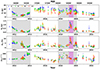 |
Fig. 1. Results of the KVN observations at 22 (blue), 43 (green), 86 (orange), and 129 GHz (red). Each panel shows the total flux density, linearly polarized flux density, polarization degree, and polarization angle (from top to bottom). The two time periods that we focus on in this work are shown in the gray shaded regions and discussed in Section 3.1. The magenta shaded area indicates a flaring period in polarized emission. |
For this study, we mainly focused on two periods, around MJD 55800–56700 and MJD 58000–58900. At the beginning of the first period, 3C 454.3 exhibits a global decrease in its flux densities, while both mp and χobs remain constant until 2013 (∼5%, ∼ 100°). After that, as polarized emission approaches its minimum state around MJD 56400, χobs rotates to ∼210°, and SI starts increasing at the same time. To investigate the jet evolution in the polarized emission during this period, we employed the VLBA 43 GHz maps and found different aspects between the core and Region C, as shown in Figure 2: the core becomes brighter, while Region C is fading out. When Region C dominates the polarized emission, it exhibits χobs ≈ 90°. However, when the core dominates the emission, χobs of the core appears ∼30° (i.e., nearly matching 210° in Figure 1). This suggests that the evolution in SI and Sp, and the rotation in χobs to ∼210° in the KVN data around MJD 56400 is the cause of the different evolution of the core and Region C.
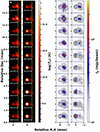 |
Fig. 2. Left: 43 GHz VLBA images in terms of the brightness temperature Tb in the source rest frame. The right ascension of the radio core is fixed to 0. The cyan contours indicate where Tb = Teq ≈ 5 × 10¹⁰ K. The yellow dashed lines present the location 0.6 mas from the core, a typical projected distance of Region C (0.45–0.7 mas; Weaver et al. 2022). Right: contours obtained from Stokes I images, starting from 3σrms level, where σrms represents the r.m.s noise level in a residual map. The color maps show linear polarization intensity. All the images are convolved with a beam size of 0.2 × 0.2 mas2. The black bars indicate the observed polarization angle on the images where the S/N of the polarized emission is higher than 3. |
In late 2018 (i.e., second period, around MJD 58400), the angle rotates from ∼150° to ∼100° at 22, 43, and 86 GHz. At 129 GHz, χobs at the beginning point deviates from 150°, but the uncertainty is quite large ( ). This rotation accompanies an increase in Sp, for example, at 129 GHz, by factors of ≳8, indicating a polarization flare. The estimated mp reaches the maximum at all frequencies (e.g., ∼10% at 129 GHz, as listed in Table B.1). We note that the increases in Sp and mp were observed at all four frequencies, and mp is clearly larger at higher frequencies around the peak of the flare. The chromatic evolution in mp is possibly related to a physical condition, for example, a shocked region (see Section 4.4.3, and see also Tavecchio et al. 2018). In addition, the overall trend in variation among polarimetric measurements at all frequencies is comparable. This implies that the flaring event and its polarization variations at 22–129 GHz originated from a common emitting region in the relativistic jet.
To investigate the resolved (high spatial resolution) polarization characteristics in the jet, the 43 GHz VLBA data was employed. The parameters (II, Ip, mp, and χobs) were first computed for each pixel in the CLEAN map, and were then averaged over the pixels associated with each model component. The pixels were chosen from a box area with dimensions matched to the full width at half maximum of the corresponding Gaussian components. The corresponding errors were estimated following Hovatta et al. (2012). The obtained values from the CLEAN flux are consistent with the KVN 43 GHz single-dish data, especially in polarized emission as described in Appendix A.
Figure 3 shows the light curves of the core (black dots) and Region C (red dots). In general, the core displays higher II than Region C, while they alternate in dominance in Ip. Several peaks are clearly identified in both II and Ip.
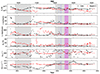 |
Fig. 3. Estimated values of the regions related to the core and Region C at 43 GHz. Each value was obtained by computing the corresponding pixels. The first four panels (from top to bottom) indicate brightness temperature, total intensity, linearly polarized intensity, and polarization degree. The last two panels are polarization angles, but the one in the bottom panel was obtained after resolving the nπ-ambiguity following the method in Blinov et al. (2016). The blue dotted and dashed lines show the ejection and segmentation time of knot B19 (Weaver et al. 2022). |
Although, in general, the core presents relatively low polarization degrees (≲5%, and mean value of  ), the χobs of the core suggests rapid variation with 180° ambiguity to adjacent data points (i.e., in time). After resolving the nπ-ambiguity by assuming the continuous variation described in Section 3.1, we obtained a swing (approximately from −200° to +400°) of χobs from the core region on a long timescale.
Regarding Region C, the overall polarization degree mp is higher than at the core, with the maximum value reaching ∼20% (and mean value of  ). The large uncertainties on mp arise when the signal-to-noise ratio of Region C is low. Interestingly, the χobs of this region is aligned to be ∼100° in a high-polarization state (e.g., ≳200 mJy/beam) and deviates from that in low-polarization (e.g., < 200 mJy/beam) periods. In addition, several clear peaks in the polarized emission of Region C seem to have appeared after the flaring activities in the core. Given that Region C is the downstream region beyond the core, it is plausible to interpret that a moving knot induces activity when the knot arrives at Region C. Jeong et al. (2023) suggested that the γ-ray flare in August 2015 (about MJD 57250) is attributed to knot K14 (B12 knot defined in Weaver et al. 2022) when it arrived at Region C.
Correlations between the polarimetric measurements obtained from the KVN single-dish and the VLBA were investigated, as shown in Figure 4: SI/χobs–Sp and II/χobs–Ip (left) and mp–χobs (right). χobs measured from the KVN were distributed with respect to ∼100° at all four frequencies when Sp was bright. Similar behavior was also found in Region C. The right panel also confirms this behavior of χobs. These data indicate that a physical process increasing the polarized emission in Region C causes the observed relations.
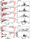 |
Fig. 4. Left: dependence of total emission (black symbols) and χobs (red symbols) on polarized emission for the KVN data at different frequencies (first four panels) and the two different jet regions from the VLBA 43 GHz, the core and Region C (last two panels). Right: dependence of mp on χobs. |
3.2. Polarization angle and rotation measure
In this section, we present the results of RM using the KVN single-dish data. RM is a measurement that shows the Faraday screening effect of a foreground medium. As noted in Equation (1) (RM ∝ ∫neB∥dl), high RM indicates high ne, strong B∥, or both. Figure 5a presents the RMs obtained from a linear model fitting. The RMs are shown in log scale to illustrate the variation in magnitude, while the RM signs are described by red dots for a positive RM (i.e., parallel magnetic field toward us) and blue dots for a negative RM (i.e., magnetic field in the opposite direction). The number of frequencies in the linear fitting is described by filled and open circles, respectively.
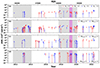 |
Fig. 5. RMs in the first panel (top) were obtained via linear fit (χ = χ0 + RM λ2) if more than two data points were available. There are several large uncertainties (σRM ≳ |RM|) attributed mainly to a significant deviation in χobs to a linear relation. From the second to the last panels, RMs were calculated in pairs of 22–43 GHz (second), 43–86 GHz (third), and 86–129 GHz (bottom). RM signs are shown in color: blue and red for negative and positive signs, respectively. The filled and open circles in the first panel indicate the number of frequencies used in the fitting, four and three data points, respectively. Each shaded area is the same as in Figure 1. |
We found that the order of RM values obtained from the linear fitting lie in a level of ∼103 rad m−2 and the mean value is approximately ( − 0.1 ± 2.7)×102 rad m−2. Several sign flips appear, but they are not significant, given their uncertainty ranges. In a previous polarization monitoring study, the averaged RM of 3C 454.3 was reported to be ( − 2 ± 52)×103 rad m−2 at 86–229 GHz (Agudo et al. 2018b). Similarly, the absolute values in RM (|RM|) suggest a variability in |RM| as well. In addition, in the fourth column in Figure B.16, multiple epochs show χobs values with large offsets from a single RM fit.
In order to focus on the epochs during which a single component dominates the polarized emission, the VLBA data was employed. For this work we studied the periods when Region C dominates the polarized emission. Based on mp obtained from the KVN and 43 GHz VLBA images (Figure C.1), several epochs were selected as C-dominating periods: from February 2019 to June 2019. During these periods, mp is high with chromatic behavior in frequency, indicating partially ordered magnetic field lines (see Figure B.1). In particular, we note that the amount of increased Sp is consistent at all frequencies and is remarkable compared to the pre-flare state. These results tentatively suggest that the polarimetric variations are mainly related to the evolution of Region C. The obtained χobs at all frequencies are aligned near 100°, but it does not follow a simple linear relation with λ2.
4. Discussion
4.1. Total and polarized brightness evolution
Figure 1 shows the time variation in flux densities (SI and Sp), polarization degree (mp), and polarization angle (χobs) obtained from the KVN multifrequency single-dish observations. In this section we discuss the variations in two periods, MJD 55800–56700 and MJD 58000–58900 (shaded in gray).
In the period of MJD 55800–56100, both SI and Sp decrease by a factor of about 0.6, while χobs remains nearly constant (i.e., ∼100°) at 22 and 43 GHz. However, starting around MJD 56300, the light curves display different evolutions between total and polarized emission with rotation in χobs from ∼100° to ∼200° : an increase in total flux density with a decrease in polarized flux density. The different evolutions are unlikely to originate from a single synchrotron emission region. If there were two or more emitting regions observed in a single-dish beam, the different evolutions in SI and Sp can be explained; for example, one region dominant in polarized emission has diminished (decreasing Sp), and then the other weakly polarized and fainter one becomes brighter and dominates the overall emission. It seems that two main regions dominate the overall emission in 3C 454.3 around this period: the core and the quasi-stationary Region C. As shown in Figure 3, while the core was bright in total intensity, the polarized intensity was predominant in Region C at the beginning of the first period. After that, Region C decayed in polarized emission with a nearly constant χobs while the core started increasing its brightness around MJD 56300.
In the beginning of the second period (MJD 58000–58900), while the source is bright in SI it is not in Sp (Figure 1). However, starting from MJD 58400, both total and polarized emission increase at all the KVN frequencies, reaching Sp ∼ 1000 mJy and mp ∼ 10% in April 2019. The obtained mp exhibits chromatic behavior during the increasing stage. The amount of increase in polarized emission is similar among the frequencies. Unlike the behavior presented in the first period, the increase in both total and polarized emission may indicate a single highly polarized synchrotron emitting region leading the polarization evolution. In addition, we found that such activity also appears in Region C with Ip > 500 mJy/beam, as shown in Figure 3; thus, in polarized emission, Region C was dominant and the core was quiet. Combining these results, we conclude that Region C is the origin of the polarization flare in 2019 at frequencies between 22 and 129 GHz.
4.2. The origin of variation in polarization angle
In this study, we applied the methodology introduced in Blinov et al. (2016) for resolving nπ-ambiguity in time as described in Section 3.1. As a cross-check, we also determined that the χobs obtained from the VLBA data agree closely with that of the KVN at 43 GHz after resolving the ambiguity (Figure A.1).
The resultant angles obtained from the KVN show several variations (Figure 1). Even with these variations the polarimetric relations of χobs reveal angles aligned to ∼100° when strongly polarized at all frequencies (Figure 4). This behavior is attributed to Region C, as described in Section 3.1, indicating that, in general, polarized emission is dominated by Region C when the source is strongly polarized.
Based on the VLBA 43 GHz data, we separately investigated the χobs of the core and Region C using the corresponding pixels where each region is located, as shown in Figure 3. Interestingly, the core seems to suggest a long-term variation in χobs after resolving a time–nπ-ambiguity. Possible explanations for this long-term variation are (i) helical magnetic field geometry with a bending within the core (for this case, one may find in Myserlis et al. 2018), (ii) rotation or ∼90° of flip in χobs by an opacity effect (Lobanov 1998; Gabuzda & Gómez 2001; Porth et al. 2011; Chamani et al. 2023), or (iii) a stochastic random walk process (Blinov et al. 2015; Kiehlmann et al. 2017). Alternatively, it is also possible that the variation in χobs is a biased result due to a relatively large cadence (about one month). Since the method we applied assumes no significant jump in χobs (> 90°) between the adjacent epochs, the related information may be biased if the intrinsic angle rotates faster than the observed cadence. For example, a rapid variation (e.g., spanning a few hours to a few days) in χobs can occur via magnetic reconnection (Zhang et al. 2018, 2020). Possibly, high-cadence and long-term VLBI observations in the future would reveal whether this long-term variation is intrinsic or not.
Meanwhile, Region C suggests a specific angle, mostly between 90° and 120°. Among the observations collected in this study, one of the periods worth noting is around April 2019, showing a prominent polarization flaring activity in Region C, as identified in Section 4.1 (see also Figure 3). As the flare grows from the beginning (∼MJD 58400), the χobs values at all frequencies rotate into a direction parallel with the jet axis (∼ − 80°, Weaver et al. 2022). This rotation in χobs with increased flux density implies a physical process in Region C. A polarization angle parallel to the jet axis is feasible through a dominant toroidal magnetic field component in the jet.
4.3. Faraday rotation measure in arcsecond scales
The polarimetric measurements (χobs and RM) used in Figure B.1 are listed in Tables B.1 and B.2. Figures 5b–d and B.2 show |RM| obtained from the KVN in the frequency domain. As presented, RM shows a large mean of |RM|≳103 rad/m2 as well as a variability not only in its magnitude, but also in its sign. These imply that an external medium is unlikely to be the main reason for the Faraday screening medium if present.
The calculated mean of |RM| in the available periods are 2.9 ± 0.2, 7.4 ± 1.3, and 32.6 ± 11.6 in units of 103 rad m−2 at 22–43, 43–86, and 86–129 GHz pairs, respectively (see Section 3.2). Although it seems to suggest frequency-dependent |RM|, one needs to be careful in interpreting frequency dependence in |RM| as systematic effects may affect |RM|.
There are several origins of the time variability and frequency dependence of RM. For example, the variability can be attributed to the dynamics in the jet, such as turbulence or helical magnetic field lines, since it depends on the direction of magnetic field lines toward us. Zamaninasab et al. (2013) found evidence of a large-scale helical field structure in the jet of 3C 454.3 through multifrequency VLBI observations.
Alternatively, we could not rule out the possible beam convolution effect (i.e., beam depolarization) on RM variability at other frequencies, although we have identified consistent polarized emission of the source on arcsecond and milliarcsecond scales at 43 GHz. The source has a complex jet structure (on milliarcsecond scale) not only in total emission, but also in polarized emission, as shown in Figures 2 and C.1. The complex jet structure with large beam sizes in the KVN single-dish observations possibly results in rotation in χobs through a beam convolution effect attributed to |RM| variation. For this reason, we selected a few epochs (from February 2019 to June 2019) in which Region C dominates the polarized emission of 3C 454.3 at 43 GHz and found the frequency dependence in |RM| in those epochs.
To understand the frequency-dependeny |RM| of 3C 454.3 shown in this work in more detail, we consider the opacity effect to χobs. As the synchrotron emission becomes optically thick at low frequency, it is possible that the opacity effect rotates χobs by about 90° (Gabuzda & Gómez 2001; Porth et al. 2011). Alternatively, the frequency dependence can be related to the core-shift effect (Lobanov 1998). As described in Jorstad et al. (2007), if the Faraday screening medium is very close to the jet, such as a sheath layer, frequency-dependent |RM| can be obtained.
However, the downstream jet, Region C, is expected to be optically thin in the KVN observing frequency range, restricting us from considering the opacity effect as the origin of the frequency-dependent |RM|. In addition, we cannot be confident if the polarized emission from the core is faint at higher frequencies (86 and 129 GHz). If the core has prominent polarized emission compared to Region C at these frequencies, then χobs may be affected by this.
We consider that the frequency-dependent |RM| shown in this work is most likely attributed to complex and unresolved polarized emission regions within 1 mas (i.e., the case of beam convolution) rather than an external Faraday screening medium. Traianou et al. (2024) studied spatially resolved polarized emission in 3C 454.3 using VLBI observations at 43 and 86 GHz. As shown in their work, the core and Region C have different spectral indices at 43 and 86 GHz: flat and thin spectra for the core and Region C, respectively, resulting in different morphologies in total intensity and polarization at 43 and 86 GHz (i.e., showing complex structure). Therefore, high-resolution multifrequency VLBI observations in full-polarization mode would be required to perform a more detailed analysis of RM variability in the jet.
4.4. Origins of a polarization flare in Region C
In Section 4.1, we identify that the flaring region is related to Region C based on a consistent evolution in flux density across the KVN frequencies, and based on the VLBA 43 GHz maps. In addition, χobs rotates from ∼150° to ∼100° during the flare. Since the core region was faint with several non-detections in polarization during this period, we interpret that the increasing |RM| with frequency and other polarimetric properties are related to a physical process in Region C. To understand this, we consider three cases: (i) jet–medium interaction, (ii) magnetic reconnection, and (iii) shock–shock interaction. Finally, we investigate how the Doppler boosting effect via a change in viewing angle can describe the observed brightness increase.
4.4.1. Jet–medium interaction
For the first scenario, a jet interacting with an ambient medium may result in a high RM. The broad-line region (BLR) and the narrow-line region (NLR) are the possible candidates for this medium. In addition, the jet can be bent toward us by the collision, leading to an increase in the Doppler factor, and thus the brightness as well. However, we note the de-projected location of Region C is dC ≈ 200 pc from the core by adopting a mean viewing angle  (see Table 12 in Weaver et al. 2022), and its projected distance from the core of ∼0.6 mas. The distance of BLR in 3C 454.3 is dBLR ≈ 0.2 pc (Bonnoli et al. 2011; Costamante et al. 2018), which was estimated using the size–luminosity relation. Moreover, based on the activity in optical line emission, Amaya-Almazán et al. (2021) interpreted that the increase in continuum emission during a flaring period (FP2, approximately 2014–2017), in which Region C brightened, was not strongly related to the BLR. Therefore, we exclude the BLR from the dense cloud candidate. If the medium corresponds to the NLR at parsec to kiloparsec scales, we expect a stable ne, B∥, and path length. In this case, the estimated RM magnitude and its sign would not vary significantly either in time or frequency. However, we would expect constant RM across the observing frequencies and time if the Faraday screening medium were related to the NLR. Therefore, we suggest that the NLR is also less likely to cause the flare with variation in RM via jet–medium collision.
4.4.2. Magnetic reconnection
Alternatively, magnetic reconnection, a physical process of rejoining two oppositely aligned magnetic field lines, can introduce increased ne, magnetic field strength, and the acceleration of plasmoids in the jet region (Zhang et al. 2018; Nathanail et al. 2020; Sironi et al. 2021). Given the magnetic energy density dominance in Region C, as reported in Jeong et al. (2023), this region is suitable for magnetic reconnection. The magnetic dominance can also be supported by having a brightness temperature (Tb) lower than the equipartition condition (Teq ≈ 5 × 10¹⁰ K, Readhead 1994). Figure C.1 shows the Tb estimated in the source rest frame. The obtained Tb of Region C was lower than Teq before a moving knot arrived in Region C, indicating a possible magnetic dominance.
By using particle-in-cell (PIC) simulations, Petropoulou et al. (2016) studied the physics of plasmoids in a relativistic jet, which is formed by the fragmentation of reconnection current sheets (current sheets derived by magnetohydrodynamic instability), which is a region containing magnetic field lines and energetic particles. From the simulation they found that the highest emission is observed when a plasmoid leaves the current sheet layer. Zhang et al. (2020) investigated the signatures in the polarization of magnetic reconnection in blazars at multiwavelengths. In their work, magnetic field lines are found to be disordered when a reconnection layer segments into several plasmoids. This results in a low mp when the observed total emission peaks due to depolarization by the tangled magnetic field lines in a plasmoid. In our study, however, we obtained increasing mp and Sp as SI increases during the flare in 2019. Therefore, we consider that magnetic reconnection is less likely to govern the physics in Region C.
4.4.3. Shock–shock interaction
In the last scenario, ne and B∥ in a jet can also be increased via shock–shock interaction, leading to the compression of a jet region. Previous studies on 3C 454.3 at high resolution have identified a quasi-stationary behavior of Region C, although a marginal motion was observed at a distance range of 0.45–0.7 mas from the core (Jorstad et al. 2017; Weaver et al. 2022). The motion is possibly related to the intrinsic physics of Region C, but as suggested in Weaver et al. (2022), it also can be explained by the relative motion of the core produced by the core-shift effect. Liodakis et al. (2020) explained the spatial variation in Region C with the emergence of a new jet component from the core.
The possibility of Region C as a recollimation or standing shock has been discussed in previous studies (Gómez et al. 1999; Jeong et al. 2023; Traianou et al. 2024). If Region C is related to a shock, its interaction with an upstream shock moving downstream is considered a shock–shock interaction. In this case, the intrinsic polarization angle of the shocked region will be parallel with the jet axis due to the compression of magnetic field components perpendicular to the jet axis (Marscher 2014) for the case of conical shock or self-generated magnetic field lines that are predominantly aligned in a direction parallel to the shock front (Tavecchio et al. 2018).
Moreover, in the shock–shock interaction scenario, a chromatic behavior in mp with observing frequency is expected based on the energy-stratified model (Tavecchio et al. 2018, 2020; Liodakis et al. 2022). In the region where the jet is most compressed, such as the Mach disk or shock front, the magnetic field lines are expected to be ordered, and thus a high mp is observed. Beyond the region (downstream of the jet), the jet expands, and the magnetic field lines are relatively disordered as it flows downstream, leading to low mp. Since high-energy electrons undergo a stronger radiative cooling process than low-energy electrons, the dominant emission region at higher frequencies is closer to the compressing region than at lower frequencies. As shown in Figure B.1 and Table B.1, mp is as high as ∼10% at high frequencies, but is rather low (∼5%) at 22 and 43 GHz during the flare. If the extended jet (e.g., ≳1 mas; see also Figure C.1) of 3C 454.3 is highly polarized, mp can be depolarized via the beam depolarization effect, especially at low frequencies. However, Sp and mp are comparable at scales between milliarcsecond and arcsecond, as shown in Figure A.1, and thus we expect the extended jet to have a negligible effect on the polarized emission at frequencies higher than 43 GHz. Furthermore, we also expect a negligible depolarization effect by turbulent magnetic fields if Region C is related to the shock interaction showing well-ordered magnetic field lines.
It is also possible that Region C is related to an oblique shock rather than a simple recollimation or standing shock. In the case of an oblique shock, the jet direction potentially varies by jet instabilities or jet bending. In particular, the jet of 3C 454.3 has a very narrow viewing angle (θv), so its brightness is sensitive to the jet flow direction via the Doppler boosting effect, as discussed in a previous study (Traianou et al. 2024). Therefore, it is essential to examine if the pure jet bending can explain the observed brightness increase during the polarization flare.
4.4.4. Changes in viewing angle
As blazar jets generally have θv smaller than 10°, a change in θv can induce strong variability. Traianou et al. (2024) suggested Region C as a bent jet region to explain the disappearance of a moving knot and brightness increase. In a similar way, we investigated the variation in Doppler factor δ to determine whether the increased SI and Sp during the flare were strongly attributable to the change in θv. As shown in Figure C.1, a plasma blob having Tb ≳ Teq was identified and ejected downstream from the core to Region C. Given its ejection time, the plasma blob is likely related to the knot B19 defined in Weaver et al. (2022). As the blob approaches Region C, Tb increases with a peak value of ∼2.6 × 10¹¹ K. Compared to the minimum peak value of the blob (Tb, min ≈ 7.3 × 10¹⁰ K) during its ejecting period, the brightness increased by a factor of more than three. After crossing Region C, the blob seems to move further downstream with reduced Tb. We note that Tb is computed in the source rest frame, so the only factors that can change Tb are particle acceleration and/or energy loss or a change in viewing angle that affects δ.
To evaluate the Doppler boosting effect by viewing angle, we adopt the apparent speed of knot B19 and the mean viewing angle of 3C 454.3 as βapp = 18 ± 1.8 and  , respectively (see Tables 8 and 12 in Weaver et al. 2022). At this angle, we obtain the bulk Lorentz factor of B19 as Γ ≈ 21.7 ± 1.4. By assuming a constant Γ of the knot during its journey, we find the ratio of the Doppler factors at viewing angles of
  and 0° to be ∼1.28 ± 0.16. Based on the observed ratio of δ higher than three, we conclude that by itself a change in θv is insufficient to describe the increased Tb, implying an additional source intrinsic process, such as particle acceleration.
Although the observational results favor an additional particle acceleration in Region C by a shock–shock interaction, the lack of emission beyond the region leaves an open question. If the region has a very steep optically thin spectrum, for example, due to a strong cooling process, this can explain the absence of emission. A high-resolution analysis at multifrequency, including low-frequency (e.g., 15 GHz), would be required to investigate spectral information beyond Region C.
5. Conclusions
In this work we studied the polarimetric variations of 3C 454.3 using decadal data (2011–2022) at millimeter wavelengths. We found several notable polarimetric features, especially in 2013–2014, and 2019. We summarize our results and conclusions as follows:
-
At all frequencies used in this work, relations between the polarimetric characteristics show a trend of χobs ≈ 100° when the polarized emission is strong (Figure 4). By analyzing the VLBA data, we found that Region C yields consistent results, indicating a prominent polarized jet region downstream of the radio core even at 129 GHz. While the χobs of Region C does not change after resolving the nπ-ambiguity in time (Blinov et al. 2016), the χobs of the radio core exhibits a large long-term swing.
-
Around 2013–2014, χobs rotated from ∼100° to ∼200° with decreasing Sp and prominent variations in |RM| at 22–43 GHz pair. From the VLBA 43 GHz data, we found that Region C dominated the polarized emission at milliarcsecond scale and then decayed in all emission (SI and Sp) during this period. At the same time, the core emission was enhanced. These imply that the rotation in χobs and the |RM| variation did not originate from a common emitting region, but can be attributed to the co-evolution of Region C and the core.
-
A notable polarization flaring event in 2019 was captured in the KVN observations. Even though this activity increased the total emission slightly, a prominent evolution appeared in the polarized emission. During the flaring period, the χobs at all the KVN observing frequencies rotated toward ∼100° with partially ordered magnetic field lines (e.g., mp ≳ 10% at 129 GHz). By investigating high angular resolution maps from the VLBA at 43 GHz, we identified that the polarization flare occurred in Region C when a moving blob (possibly related to knot B19 in Weaver et al. 2022) arrived at Region C.
-
To describe the flare in Region C and to investigate which physical process is favorable for the flare, we considered several cases: (i) jet-cloud interaction via BLR or NLR is unlikely to cause the flare based on the de-projected distance of Region C, the lack of optical line emission (Amaya-Almazán et al. 2021), and variable RM; (ii) magnetic reconnection is excluded due to the opposite evolution in mp between the PIC simulation (decreasing mp, Zhang et al. 2020) and our observations (increasing mp) during the flare; (iii) shock–shock interaction can explain the overall observational results (chromatic mp, concurrent rise in SI and mp, and χobs parallel to the jet axis) (Marscher 2014; Tavecchio et al. 2018, 2020; Liodakis et al. 2020). Therefore, we suggest that a shock–shock interaction is the most likely mechanism for the flare in 2019.
-
We also investigated a possible beaming effect caused by a local bending of the jet for some reason. The mean θv of 3C 454.3 was obtained as
 by averaging those of several knots (Weaver et al. 2022). By adopting the apparent speed of knot B19 as βapp ≈ 18 ± 1.8, we obtained the resultant Doppler factor δ ≈ 33.9 ± 4.4 for the knot. In the assumption of constant Γ of the moving knot, the Doppler factor at θv = 0° was computed to be δ0 ≈ 43.5 ± 2.8. Therefore, the change in θv toward us can increase δ by 1.28 ± 0.16, and this is insufficient to explain the observed increased brightness of about 3.5 times. Provided with this and the favored physical model, we interpret that the shock–shock interaction may be responsible for the polarization flaring activity in Region C with additional particle acceleration.
Data availiability
The Appendix B figures are available on https://zenodo.org/records/14967589
Lee et al. (2016) used 10%–30% of uncertainties in amplitude calibration. However, note that these are from VLBI observations, not single-dish observations.
Appendix B Figures are available on https://zenodo.org/records/14967589
Acknowledgments
We thank Thomas Krichbaum, Alan Marscher, and Svetlana Jorstad for reading the manuscript and helping us to improve it with valuable comments. The KVN is a facility operated by the KASI (Korea Astronomy and Space Science Institute). The KVN observations and correlations are supported through high-speed network connections among the KVN sites provided by the KREONET (Korea Research Environment Open NETwork), which is managed and operated by KISTI (Korea Institute of Science and Technology Information). This work was supported by the National Research Foundation of Korea (NRF) grant funded by the Korea government (MIST) (2020R1A2C2009003, RS-2025-00562700). We also acknowledge financial support from the National Research Foundation of Korea (NRF) grant 2022R1F1A1075115. This study makes use of VLBA data from the VLBA-BU Blazar Monitoring Program (BEAM-ME and VLBA-BU-BLAZAR; http://www.bu.edu/blazars/BEAM-ME.html), funded by NASA through the Fermi Guest Investigator Program. The VLBA is an instrument of the National Radio Astronomy Observatory. The National Radio Astronomy Observatory is a facility of the National Science Foundation operated by Associated Universities, Inc. This work made use of Astropy: (http://www.astropy.org) a community-developed core Python package and an ecosystem of tools and resources for astronomy (Astropy Collaboration 2013, 2018, 2022).
References
- Agudo, I., Thum, C., Wiesemeyer, H., et al. 2012, A&A, 541, A111 [NASA ADS] [CrossRef] [EDP Sciences] [Google Scholar]
- Agudo, I., Thum, C., Molina, S. N., et al. 2018a, MNRAS, 474, 1427 [NASA ADS] [CrossRef] [Google Scholar]
- Agudo, I., Thum, C., Ramakrishnan, V., et al. 2018b, MNRAS, 473, 1850 [Google Scholar]
- Amaya-Almazán, R. A., Chavushyan, V., & Patiño-Álvarez, V. M. 2021, ApJ, 906, 5 [Google Scholar]
- Angelakis, E., Hovatta, T., Blinov, D., et al. 2016, MNRAS, 463, 3365 [NASA ADS] [CrossRef] [Google Scholar]
- Astropy Collaboration (Robitaille, T. P., et al.) 2013, A&A, 558, A33 [NASA ADS] [CrossRef] [EDP Sciences] [Google Scholar]
- Astropy Collaboration (Price-Whelan, A. M., et al.) 2018, AJ, 156, 123 [Google Scholar]
- Astropy Collaboration (Price-Whelan, A. M., et al.) 2022, ApJ, 935, 167 [NASA ADS] [CrossRef] [Google Scholar]
- Aumont, J., Conversi, L., Thum, C., et al. 2010, A&A, 514, A70 [NASA ADS] [CrossRef] [EDP Sciences] [Google Scholar]
- Blinov, D., & Pavlidou, V. 2019, Galaxies, 7, 46 [NASA ADS] [CrossRef] [Google Scholar]
- Blinov, D., Pavlidou, V., Papadakis, I., et al. 2015, MNRAS, 453, 1669 [NASA ADS] [CrossRef] [Google Scholar]
- Blinov, D., Pavlidou, V., Papadakis, I., et al. 2016, MNRAS, 462, 1775 [Google Scholar]
- Bonnoli, G., Ghisellini, G., Foschini, L., Tavecchio, F., & Ghirlanda, G. 2011, MNRAS, 410, 368 [NASA ADS] [CrossRef] [Google Scholar]
- Burn, B. J. 1966, MNRAS, 133, 67 [Google Scholar]
- Buson, S. 2014, The Astronomer’s Telegram, 6236, 1 [Google Scholar]
- Chamani, W., Savolainen, T., Ros, E., et al. 2023, A&A, 672, A130 [NASA ADS] [CrossRef] [EDP Sciences] [Google Scholar]
- Clark, B. G. 1980, A&A, 89, 377 [NASA ADS] [Google Scholar]
- Cornwell, T., Braun, R., & Briggs, D. S. 1999, in Synthesis Imaging in Radio Astronomy II, eds. G. B. Taylor, C. L. Carilli, & R. A. Perley, ASP Conf. Ser., 180, 151 [Google Scholar]
- Costamante, L., Cutini, S., Tosti, G., Antolini, E., & Tramacere, A. 2018, MNRAS, 477, 4749 [Google Scholar]
- Dahal, S., Brewer, M. K., Akins, A. B., et al. 2023, PSJ, 4, 154 [Google Scholar]
- de Pater, I., Sault, R. J., Moeckel, C., et al. 2019, AJ, 158, 139 [Google Scholar]
- Di Gesu, L., Donnarumma, I., Tavecchio, F., et al. 2022, ApJ, 938, L7 [CrossRef] [Google Scholar]
- Gabuzda, D. C., & Gómez, J. L. 2001, MNRAS, 320, L49 [Google Scholar]
- Gómez, J.-L., Marscher, A. P., & Alberdi, A. 1999, ApJ, 522, 74 [CrossRef] [Google Scholar]
- Högbom, J. A. 1974, A&AS, 15, 417 [Google Scholar]
- Hovatta, T., Lister, M. L., Aller, M. F., et al. 2012, AJ, 144, 105 [Google Scholar]
- Hovatta, T., O’Sullivan, S., Martí-Vidal, I., Savolainen, T., & Tchekhovskoy, A. 2019, A&A, 623, A111 [NASA ADS] [CrossRef] [EDP Sciences] [Google Scholar]
- Hull, C. L. H., & Plambeck, R. L. 2015, Journal of Astronomical Instrumentation, 4, 1550005 [Google Scholar]
- Jeong, H.-W., Lee, S.-S., Cheong, W. Y., et al. 2023, MNRAS, 523, 5703 [Google Scholar]
- Jorstad, S. G., Marscher, A. P., Lister, M. L., et al. 2005, AJ, 130, 1418 [Google Scholar]
- Jorstad, S. G., Marscher, A. P., Stevens, J. A., et al. 2007, AJ, 134, 799 [NASA ADS] [CrossRef] [Google Scholar]
- Jorstad, S. G., Marscher, A. P., Smith, P. S., et al. 2013, ApJ, 773, 147 [Google Scholar]
- Jorstad, S., Larionov, V., Mokrushina, A., Troitsky, I., & Morozova, D. 2015, The Astronomer’s Telegram, 7942, 1 [Google Scholar]
- Jorstad, S. G., Marscher, A. P., Morozova, D. A., et al. 2017, ApJ, 846, 98 [Google Scholar]
- Kam, M., Trippe, S., Byun, D.-Y., et al. 2023, Journal of Korean Astronomical Society, 56, 1 [Google Scholar]
- Kang, S., Lee, S.-S., & Byun, D.-Y. 2015, Journal of Korean Astronomical Society, 48, 257 [Google Scholar]
- Kemball, A. J., Diamond, P. J., & Pauliny-Toth, I. I. K. 1996, ApJ, 464, L55 [Google Scholar]
- Kiehlmann, S., Savolainen, T., Jorstad, S. G., et al. 2016, A&A, 590, A10 [NASA ADS] [CrossRef] [EDP Sciences] [Google Scholar]
- Kiehlmann, S., Blinov, D., Pearson, T. J., & Liodakis, I. 2017, MNRAS, 472, 3589 [Google Scholar]
- Kim, D. E., Di Gesu, L., Liodakis, I., et al. 2024, A&A, 681, A12 [NASA ADS] [CrossRef] [EDP Sciences] [Google Scholar]
- Kuo, C. Y., Asada, K., Rao, R., et al. 2014, ApJ, 783, L33 [NASA ADS] [CrossRef] [Google Scholar]
- Kutkin, A. M., Sokolovsky, K. V., Lisakov, M. M., et al. 2014, MNRAS, 437, 3396 [Google Scholar]
- Lee, S.-S., Wajima, K., Algaba, J.-C., et al. 2016, ApJS, 227, 8 [Google Scholar]
- Liodakis, I., Blinov, D., Jorstad, S. G., et al. 2020, ApJ, 902, 61 [NASA ADS] [CrossRef] [Google Scholar]
- Liodakis, I., Marscher, A. P., Agudo, I., et al. 2022, Nature, 611, 677 [CrossRef] [Google Scholar]
- Lister, M. L., Aller, M. F., Aller, H. D., et al. 2018, ApJS, 234, 12 [CrossRef] [Google Scholar]
- Lister, M. L., Homan, D. C., Kellermann, K. I., et al. 2021, ApJ, 923, 30 [NASA ADS] [CrossRef] [Google Scholar]
- Lobanov, A. P. 1998, A&A, 330, 79 [NASA ADS] [Google Scholar]
- Marinucci, A., Muleri, F., Dovciak, M., et al. 2022, MNRAS, 516, 5907 [NASA ADS] [CrossRef] [Google Scholar]
- Marscher, A. P. 2014, ApJ, 780, 87 [Google Scholar]
- Martí-Vidal, I., Muller, S., Vlemmings, W., Horellou, C., & Aalto, S. 2015, Science, 348, 311 [Google Scholar]
- Middei, R., Liodakis, I., Perri, M., et al. 2023a, ApJ, 942, L10 [NASA ADS] [CrossRef] [Google Scholar]
- Middei, R., Perri, M., Puccetti, S., et al. 2023b, ApJ, 953, L28 [NASA ADS] [CrossRef] [Google Scholar]
- Mohan, P., Agarwal, A., Mangalam, A., et al. 2015, MNRAS, 452, 2004 [NASA ADS] [CrossRef] [Google Scholar]
- Myserlis, I., Komossa, S., Angelakis, E., et al. 2018, A&A, 619, A88 [NASA ADS] [CrossRef] [EDP Sciences] [Google Scholar]
- Nagai, H., Nakanishi, K., Paladino, R., et al. 2016, ApJ, 824, 132 [NASA ADS] [CrossRef] [Google Scholar]
- Nathanail, A., Fromm, C. M., Porth, O., et al. 2020, MNRAS, 495, 1549 [Google Scholar]
- Ojha, R. 2016, The Astronomer’s Telegram, 9190, 1 [Google Scholar]
- Panebianco, G., Bulgarelli, A., Pittori, C., et al. 2022, The Astronomer’s Telegram, 15782, 1 [Google Scholar]
- Park, J., Kam, M., Trippe, S., et al. 2018, ApJ, 860, 112 [Google Scholar]
- Peirson, A. L., Negro, M., Liodakis, I., et al. 2023, ApJ, 948, L25 [NASA ADS] [CrossRef] [Google Scholar]
- Perley, R. A., & Butler, B. J. 2013, ApJS, 206, 16 [Google Scholar]
- Petropoulou, M., Giannios, D., & Sironi, L. 2016, MNRAS, 462, 3325 [NASA ADS] [CrossRef] [Google Scholar]
- Planck Collaboration XXVI. 2016, A&A, 594, A26 [NASA ADS] [CrossRef] [EDP Sciences] [Google Scholar]
- Porth, O., Fendt, C., Meliani, Z., & Vaidya, B. 2011, ApJ, 737, 42 [Google Scholar]
- Pushkarev, A. B., Hovatta, T., Kovalev, Y. Y., et al. 2012, A&A, 545, A113 [NASA ADS] [CrossRef] [EDP Sciences] [Google Scholar]
- Pushkarev, A. B., Aller, H. D., Aller, M. F., et al. 2023, MNRAS, 520, 6053 [NASA ADS] [CrossRef] [Google Scholar]
- Readhead, A. C. S. 1994, ApJ, 426, 51 [Google Scholar]
- Rybicki, G. B., & Lightman, A. P. 1979, Radiative Processes in Astrophysics (New York: Wiley) [Google Scholar]
- Shepherd, M. C. 1997, in Astronomical Data Analysis Software and Systems VI, eds. G. Hunt, & H. Payn, ASP Conf. Ser., 125, 77 [NASA ADS] [Google Scholar]
- Sironi, L., Rowan, M. E., & Narayan, R. 2021, ApJ, 907, L44 [CrossRef] [Google Scholar]
- Sokoloff, D. D., Bykov, A. A., Shukurov, A., et al. 1998, MNRAS, 299, 189 [Google Scholar]
- Tavecchio, F., Landoni, M., Sironi, L., & Coppi, P. 2018, MNRAS, 480, 2872 [NASA ADS] [CrossRef] [Google Scholar]
- Tavecchio, F., Landoni, M., Sironi, L., & Coppi, P. 2020, MNRAS, 498, 599 [NASA ADS] [CrossRef] [Google Scholar]
- Traianou, E., Krichbaum, T. P., Gómez, J. L., et al. 2024, A&A, 682, A154 [NASA ADS] [CrossRef] [EDP Sciences] [Google Scholar]
- Trippe, S. 2014, Journal of Korean Astronomical Society, 47, 15 [Google Scholar]
- Weaver, Z. R., Jorstad, S. G., Marscher, A. P., et al. 2022, ApJS, 260, 12 [NASA ADS] [CrossRef] [Google Scholar]
- Weiland, J. L., Odegard, N., Hill, R. S., et al. 2011, ApJS, 192, 19 [Google Scholar]
- Zamaninasab, M., Savolainen, T., Clausen-Brown, E., et al. 2013, MNRAS, 436, 3341 [Google Scholar]
- Zhang, H., Li, X., Guo, F., & Giannios, D. 2018, ApJ, 862, L25 [NASA ADS] [CrossRef] [Google Scholar]
- Zhang, H., Li, X., Giannios, D., et al. 2020, ApJ, 901, 149 [CrossRef] [Google Scholar]
Appendix A: Comparison of emission on milliarcsecond and arcsecond scales
The main beam sizes of the KVN single-dish and of the VLBA are largely different. This possibly causes the additional detection of extended jet structures in the KVN observations, leading to differences in polarization characteristics. To investigate, we checked the consistency between the two data sets. To do that, we compared the light curves obtained from the KVN and the VLBA at 43 GHz (Figure A.1). Each panel shows the observed values as in Figure 1. The total flux density SI of the KVN is generally higher than that of the VLBA (by a factor of 1.49 ± 0.07). However, the polarized flux density Sp is notably comparable (by a factor of 1.02 ± 0.07). This indicates that the extended jet beyond the VLBA main beam size has a weak or negligible impact on Sp. Polarization angle depends on the ratio of the Stokes U and Q (χ = 0.5tan−1(U/Q)), so χobs may differ if there is a discrepancy between the Stokes parameters, even when the polarized flux density is comparable. From the comparison of the χobs measurements, we found consistency between the two instruments. Therefore, we conclude that the obtained polarimetric features arise from the region within milliarcsecond-scale with negligible impact from the extended downstream jet. The polarization degree mp is slightly lower in the KVN data due to its high SI.
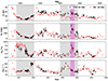 |
Fig. A.1. Comparison of the light curves at 43 GHz obtained from the KVN single-dish (black) and the VLBA (red). The flux density from the VLBA observations was estimated using the CLEAN models. |
Appendix B: Polarization angle and rotation measure of multiwavelength available epochs
We note that all Figures in Appendix B are available on 10.5281/zenodo.14967589. Figure B.1 presents the results of only 4-frequency-available epochs. In the first (flux density, Jy) and second (spectral index, Sν ∝ να) columns, the values of total and polarized emission densities are indicated by filled and open circles, respectively. The red dashed line in the second column indicates where α = 0. In the third column, the polarization degree is shown on a fixed scale (0–12) in units of percent (%). In the fourth column, the obtained polarization angle (χobs) is shown with the RM-fit (χ0 = χ + RM λ2) result as the red solid line in the squared wavelength (λ2) domain. The calculated RM value is noted in units of 103 rad m−2 in each panel. Although there are several epochs in which the linear fit well describes χobs (i.e., constant RM), for some epochs, it cannot fit the observations. To investigate a possible frequency dependence of |RM|, we calculated RM at each adjacent frequency pair, as shown in the last column. The frequency in that column is the mean frequency of the pair (νmean). The red solid line indicates the fit result of |RM|∝νa, and the resultant a index is shown in each panel. The gray shaded area indicates the range of fitted RM in absolute value (i.e., |RMfit|). Not only the full-frequency-available |RM| but also three-frequency-available results are presented in Figure B.2. In many of the epochs, |RM| seems to increase as the pair frequency (i.e., νmean) increases.
Observed polarization degrees and polarization angles from the KVN single-dish shown in Figure B.1.
Obtained values of the Faraday rotation measure and a index. The selected epochs are the same as those listed in Table B.1
Appendix C: VLBA 43 GHz images during polarization flare
All Tables
Observed polarization degrees and polarization angles from the KVN single-dish shown in Figure B.1.
Obtained values of the Faraday rotation measure and a index. The selected epochs are the same as those listed in Table B.1
All Figures
|
Fig. 1. Results of the KVN observations at 22 (blue), 43 (green), 86 (orange), and 129 GHz (red). Each panel shows the total flux density, linearly polarized flux density, polarization degree, and polarization angle (from top to bottom). The two time periods that we focus on in this work are shown in the gray shaded regions and discussed in Section 3.1. The magenta shaded area indicates a flaring period in polarized emission. |
| In the text | |
|
Fig. 2. Left: 43 GHz VLBA images in terms of the brightness temperature Tb in the source rest frame. The right ascension of the radio core is fixed to 0. The cyan contours indicate where Tb = Teq ≈ 5 × 10¹⁰ K. The yellow dashed lines present the location 0.6 mas from the core, a typical projected distance of Region C (0.45–0.7 mas; Weaver et al. 2022). Right: contours obtained from Stokes I images, starting from 3σrms level, where σrms represents the r.m.s noise level in a residual map. The color maps show linear polarization intensity. All the images are convolved with a beam size of 0.2 × 0.2 mas2. The black bars indicate the observed polarization angle on the images where the S/N of the polarized emission is higher than 3. |
| In the text | |
|
Fig. 3. Estimated values of the regions related to the core and Region C at 43 GHz. Each value was obtained by computing the corresponding pixels. The first four panels (from top to bottom) indicate brightness temperature, total intensity, linearly polarized intensity, and polarization degree. The last two panels are polarization angles, but the one in the bottom panel was obtained after resolving the nπ-ambiguity following the method in Blinov et al. (2016). The blue dotted and dashed lines show the ejection and segmentation time of knot B19 (Weaver et al. 2022). |
| In the text | |
|
Fig. 4. Left: dependence of total emission (black symbols) and χobs (red symbols) on polarized emission for the KVN data at different frequencies (first four panels) and the two different jet regions from the VLBA 43 GHz, the core and Region C (last two panels). Right: dependence of mp on χobs. |
| In the text | |
|
Fig. 5. RMs in the first panel (top) were obtained via linear fit (χ = χ0 + RM λ2) if more than two data points were available. There are several large uncertainties (σRM ≳ |RM|) attributed mainly to a significant deviation in χobs to a linear relation. From the second to the last panels, RMs were calculated in pairs of 22–43 GHz (second), 43–86 GHz (third), and 86–129 GHz (bottom). RM signs are shown in color: blue and red for negative and positive signs, respectively. The filled and open circles in the first panel indicate the number of frequencies used in the fitting, four and three data points, respectively. Each shaded area is the same as in Figure 1. |
| In the text | |
|
Fig. A.1. Comparison of the light curves at 43 GHz obtained from the KVN single-dish (black) and the VLBA (red). The flux density from the VLBA observations was estimated using the CLEAN models. |
| In the text | |
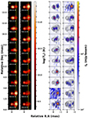 |
Fig. C.1. Same as in Figure 2, but for the period around the flare in 2019. |
| In the text | |
Current usage metrics show cumulative count of Article Views (full-text article views including HTML views, PDF and ePub downloads, according to the available data) and Abstracts Views on Vision4Press platform.
Data correspond to usage on the plateform after 2015. The current usage metrics is available 48-96 hours after online publication and is updated daily on week days.
Initial download of the metrics may take a while.