| Issue |
A&A
Volume 696, April 2025
|
|
|---|---|---|
| Article Number | A48 | |
| Number of page(s) | 13 | |
| Section | Extragalactic astronomy | |
| DOI | https://doi.org/10.1051/0004-6361/202452746 | |
| Published online | 01 April 2025 | |
Estimating masses of supermassive black holes in active galactic nuclei from the Hα emission line
1
Dipartimento di Fisica e Astronomia “G. Galilei”, Università di Padova, Vicolo dell’Osservatorio 3, I-35122 Padova, Italy
2
INAF – Osservatorio Astronomico di Padova, Vicolo dell’Osservatorio 5, I-35122 Padova, Italy
3
Jeremiah Horrocks Institute, University of Central Lancashire, Preston PR1 2HE, UK
4
c/o Tracy L. Turner, 205 South Prospect Street, Granville, OH 43023, USA
5
Department of Astronomy, University of Wisconsin – Madison, Sterling Hall, 475 N. Charter St., Madison, WI 53706-1507, USA
6
European Southern Observatory, Alonso de Córdova 3107, Casilla 19, Santiago 19001, Chile
7
Department of Astronomy and Astrophysics, Eberly College of Science, The Pennsylvania State University, 525 Davey Laboratory, University Park, PA 16802, USA
8
Institute for Gravitation and the Cosmos, The Pennsylvania State University, University Park, PA 16802, USA
9
Department of Physics, The Pennsylvania State University, 525 Davey Laboratory, University Park, PA 16802, USA
10
Università degli studi dell’Insubria, Via Valleggio 11, Como 22100, Italy
11
Osservatorio Astronomico di Brera, Istituto Nazionale di Astrofisica (INAF), Via E. Bianchi 46, Merate 23807, Italy
12
Max Planck Institute for Extraterrestrial Physics, Giessenbachstrasse, 85741 Garching bei München, Germany
13
Department of Physics, Virginia Tech, Blacksburg, VA 24061, USA
14
Eureka Scientific Inc., 2452 Delmer St. Suite 100, Oakland, CA 94602, USA
15
Instituto de Astronomía y Ciencias Planetarias, Universidad de Atacama, Copayapu 485, Copiapó, Chile
16
Kavli Institute for Astronomy and Astrophysics, Peking University, Beijing 100871, China
17
Department of Astronomy, School of Physics, Peking University, Beijing 100871, China
18
SUPA School of Physics and Astronomy, North Haugh, St. Andrews, KY16 9SS Scotland, UK
19
INAF – Osservatorio Astronomico di Capodimonte, Via Moiariello 16, 80131 Napoli, Italy
20
INAF – Osservatorio Astronomico d’Abruzzo, Via M. Maggini snc, I-64100 Teramo, Italy
21
Department of Astronomy, University of Illinois Urbana-Champaign, Urbana, IL 61801, USA
22
National Center for Supercomputing Applications, University of Illinois Urbana-Champaign, Urbana, IL 61801, USA
23
DARK, Niels Bohr Institute, University of Copenhagen, Jagtvej 155, DK-2200 Copenhagen, Denmark
24
Steward Observatory, University of Arizona, 933 N. Cherry Ave., Tucson, AZ 85721, USA
⋆ Corresponding author; This email address is being protected from spambots. You need JavaScript enabled to view it.
Received:
25
October
2024
Accepted:
23
January
2025
Abstract
Aims. The goal of this project is to construct an estimator for the masses of supermassive black holes in active galactic nuclei (AGNs) based on the broad Hα emission line.
Methods. We made use of published reverberation mapping data. We remeasured all Hα time lags from the original data as we find that reverberation measurements are often improved by detrending the light curves.
Results. We produced mass estimators that require only the Hα luminosity and the width of the Hα emission line as characterized by either the full width at half maximum or the line dispersion.
Conclusions. It is possible, on the basis of a single spectrum covering the Hα emission line, to estimate the mass of the central supermassive black hole in AGNs with all three parameters believed to affect mass measurement – luminosity, line width, and Eddington ratio – taken into account. The typical formal accuracy in such estimates is of order 0.2–0.3 dex relative to the reverberation-based masses.
Key words: galaxies: active / galaxies: nuclei / quasars: emission lines / galaxies: Seyfert
Retired.
© The Authors 2025
 Open Access article, published by EDP Sciences, under the terms of the Creative Commons Attribution License (https://creativecommons.org/licenses/by/4.0), which permits unrestricted use, distribution, and reproduction in any medium, provided the original work is properly cited.
This article is published in open access under the Subscribe to Open model. This email address is being protected from spambots. You need JavaScript enabled to view it. to support open access publication.
1. Introduction
Astrophysical masses are measured by observing how they accelerate nearby objects. In the case of supermassive black holes at the centres of massive galaxies, masses are measured by modelling the dynamics of stars (e.g. van der Marel et al. 1998; Cretton et al. 1999; Gebhardt et al. 2003; Thomas et al. 2004; Valluri et al. 2004; Sharma et al. 2014), gas (e.g. Macchetto et al. 1997; Bower et al. 1998; Davies et al. 2004a,b; Davis et al. 2013; de Francesco et al. 2008; Hicks & Malkan 2008; Dalla Bontà et al. 2009) or megamasers (e.g. Wagner 2013; van den Bosch et al. 2016; Kuo et al. 2020) on spatially resolved scales. In the case of some relatively nearby active galactic nuclei (AGNs), the broad-line-emitting gas can be spatially resolved with interferometry (GRAVITY Collaboration 2018, 2020, 2021a,b, 2024). In other cases, the motions of gas on spatially unresolved scales can be modelled for mass measurement via the process of reverberation mapping (RM; Pancoast et al. 2011; Grier et al. 2013b, 2017a; Pancoast et al. 2014). The ultraviolet, optical, and infrared spectra of AGNs are dominated by the presence of strong, Doppler-broadened emission lines whose flux varies in response to continuum variations that arise on accretion-disk scales. By mapping the response of the line-emitting gas as a function of line-of-sight velocity and time delay relative to the continuum variations, the kinematics of the line-emitting region and the mass of the central black hole can be determined. However, the technical demands of velocity-resolved (i.e. ‘two-dimensional’) RM are formidable compared to simpler measurement of the mean emission-line response time, or time lag, for an entire emission line (τ) and the emission-line width (ΔV; i.e. ‘one-dimensional RM’; Blandford & McKee 1982; Peterson 1993, 2014) Compared to one-dimensional RM, two-dimensional RM requires more accurate relative flux calibration (including flat-fielding) as well as more accurate wavelength calibration and consistent spectral resolution. It has therefore been more common to measure the one-dimensional response of the emission line and the line width and combine them to determine the black-hole mass:
 (1)
(1)
where the quantity in parentheses, known as the ‘virial product’ (μ), is in units of mass and is based on the two observables, line width and mean time delay. Under most circumstances (e.g. except when the continuum radiation or emission-line response is highly asymmetric), the mean time delay translates immediately into the mean radius of the line-emitting region, R = cτ. Parameters that are not directly measured by this method, such as the inclination of the line-emitting region, are subsumed into the dimensionless factor f. In the absence of knowledge of these other parameters, it is common to use a mean value, ⟨f⟩, based on other statistical estimates of the masses, nearly always the relationship between the black-hole mass and the bulge stellar velocity dispersion, MBH–σ*. This relationship was first recognized in quiescent galaxies (Ferrarese & Merritt 2000; Gebhardt et al. 2000a) but has also been identified in active galaxies (Gebhardt et al. 2000b; Ferrarese et al. 2001; Nelson et al. 2004; Watson et al. 2008; Grier et al. 2013a).
Even one-dimensional RM is resource-intensive, typically requiring a sequence of at least 30–50 high-quality spectroscopic observations over a suitable span of time (typically several times the light-crossing time, τ = R/c) with an appropriate sampling rate (a sampling interval typically around 0.5R/c or less) and source variations that are conducive to successful reverberation detection. Fortunately, however, RM has shown that the emission-line region radii inferred from lags correlate with many different luminosity measures (L) approximately as L ∝ R1/2, thus enabling estimates of the central black-hole mass from a single spectroscopic observation. As the RM database has grown over time, it has become clear that this radius–luminosity (R–L) relation is oversimplified and that there is at least one more parameter that affects the radius of the line-emitting region, hereafter referred to as the broad-line region (BLR). The additional parameter is generally thought to be the Eddington ratio (i.e. the ratio of the true accretion rate to the Eddington accretion rate; e.g. Du et al. 2016, 2018; Du & Wang 2019; Grier et al. 2017b; Martínez-Aldama et al. 2019; Fonseca Alvarez et al. 2020). There is a long history of using the R–L scaling relation to estimate the BLR radius from a measured luminosity and combining this with the emission-line width to estimate the mass via Eq. (1), much of which we reviewed in our earlier paper (Dalla Bontà et al. 2020, hereafter Paper I). Our investigation reported in Paper I supports the conclusion that the Eddington ratio is the missing parameter in the R–L relationship and demonstrates that this can be effectively be taken into account. In Paper I, we focused on updating the R–L relations for Hβ and C IVλ1549; the former because it has by far the best established RM database, and the latter because it affords a probe of the higher-redshift Universe and has been, we think unfairly, as we discuss in Paper I, deemed by some authors to be insufficiently reliable for mass estimates.
In the present work we focus on the other strong emission line in the optical, Hα λ6563. Compared to other strong broad emission lines in AGN spectra, Hα has been relatively neglected in RM studies. There are several reasons for this:
-
The sensitivity of the UV/optical detectors generally employed in ground-based RM studies limits the redshift range over which Hα can be observed. In the samples discussed in this paper, the highest-redshift AGNs are at z ≲ 0.15.
-
The low space density of local highly luminous AGNs combined with cosmic downsizing means that the luminosity range that can be studied via Hα reverberation is limited compared to other broad emission lines. In the samples discussed here, there is only one AGN (3C 273 = PG 1226+023) with rest-frame 5100 Å luminosity at L(5100 Å) = λLλ(5100 Å) > 1045 erg s−1 and a small handful with L(5100 Å) > 1044 erg s−1.
Other deficiencies relative to Hβ (in some cases, but not all, Hβ and Hα are observed simultaneously) are as follows:
-
The amplitude of emission-line flux variability is generally higher in Hβ than in Hα (e.g. Peterson et al. 2004), which makes the variations easier to detect and characterize.
-
The continuum underneath Hα has more host-galaxy starlight contamination than that under Hβ, so the continuum variations are apparently stronger in the Hβ region of the spectrum and the starlight correction to the continuum luminosity at Hα is much larger and thus uncertainties are more impactful.
-
In many, but not all, cases, the highest fidelity relative flux calibration in the Hβ spectral region is achieved by assuming that the [O III] λλ4959, 5007 fluxes are constant on reverberation timescales. These lines are more clearly separated from Hβ than potential narrow-line calibration sources around Hα (specifically [N II] λλ6548, 6583 or [S II] λλ6716, 6731). The [N II] lines in particular are much harder to separate from the Hα broad emission, which compromises them as internal flux calibrators and complicates measuring the broad Hα line width accurately. For two-dimensional reverberation studies (i.e. those that enable constructions of a velocity-delay map), the [N II] lines can be especially problematic.
-
At some modest redshifts, the Hα profile is badly contaminated by atmospheric absorption bands (i.e. the A band and B band), and accounting for this is not trivial.
However, recent developments in the study of nearby AGNs at high angular resolution in the near-infrared with both ground-based (e.g. GRAVITY at the VLTI) and space-based (JWST) telescopes has led to a renewed interest in reverberation results for Hα for direct comparison with mass determinations based on angularly resolved methods. For this reason, we decided to reconsider the issue of estimating AGN black-hole masses based on the Hα emission line. Our methodology largely follows that of Paper I. For consistency with Paper I, we assume H0 = 72 km s−1 Mpc−1, Ωmatter = 0.3, and ΩΛ = 0.7.
2. Observational database and methodology
2.1. Data
As in Paper I, we employed two high-quality databases for this investigation. First, we collected spectra, line-width measurements, and time series for reverberation-mapped AGNs that have appeared in the literature up through 2019. The objects included here are those from Paper I that also have Hα results available. Second, we included sources from the Sloan Digital Sky Survey Reverberation Mapping Project (hereafter SDSS-RM; Shen et al. 2015). While Paper I included only results from the first year of the project, here we examined the six-year database described by Shen et al. (2024), though as we explain below, only the first two years of spectroscopic monitoring plus a previous year of photometric monitoring are relevant to the present investigation.
Whenever possible, we used line-width measurements and flux or luminosity measurements from the published sources. In some cases where we had ready access to the data (notably the Palomar–Green quasars from Kaspi et al. 2000), we measured the line widths ourselves. In all cases, however, we remeasured the emission-line lags using the interpolated cross-correlation methodology (Gaskell & Peterson 1987) as implemented by Peterson et al. (1998) and modified by Peterson et al. (2004). We chose to remeasure all the SDSS-RM lags for two reasons.
Firstly, as described by Edelson et al. (2024), it is important to examine the effects of ‘detrending’ the light curves. Detrending means either fitting a low-order polynomial to the light curve and subtracting it from the data or convolving the light curve with a broad function, such as a Gaussian: either will remove the longest-term trends from the data. We did this because variations on timescales much longer than reverberation timescales can, because they contain so much power, lead to overestimates of the reverberation response timescale. Here we attempted a simple linear detrending, following Edelson et al. (2024), of the line and continuum light curves and used the time series that gives the ‘best’ results (generally defined by the smallest uncertainties in the lags). Typically we find that shorter light curves are unaffected by detrending, but in longer light curves the effects can be important.
Secondly, in the case of SDSS-RM data, we restricted our analysis to the first two years of spectroscopic observations (56660 < MJD < 57195) plus a preceding single year (56358 < MJD < 56508) of continuum measurements. Because the SDSS-RM quasars with Hα reverberation measurements are all fairly local and low luminosity, the sparse sampling of the continuum at earlier epochs and the continuum and lines at later epochs only adds noise to the cross-correlation results.
The data drawn from the literature are presented in Table A.1. Additional parameters associated with each source are drawn from Table A1 of Paper I1. As noted above, all lags were remeasured, but luminosities, adjusted to our adopted cosmology, and line widths are taken from the published sources. Some line-width measures were flagged by the original investigators as being particularly uncertain, usually because of various data quality issues. These values are denoted by preceding colons and are not used in any of the statistical analysis.
Table B.1 presents the parameter values for the SDSS-RM sample. Some additional necessary parameters appear in Table A2 of Paper I. Luminosities are based on parameters given by Shen et al. (2024), line widths are from Wang et al. (2019), and the Hα rest-frame lags are based on our own re-determinations. We give the range of epochs used in Col. 2 of Table B.1; we, however, eliminated epoch MJD 56713 from all the light curves as in many cases it was a clear outlier. The time span used for each individual source was the subset that gave the clearest results (i.e. those with the smallest errors and/or the least contamination by aliases).
2.2. Fitting methodology
In the remainder of this paper, we examine the relationships among various physical parameters via bivariate and multivariate fits, first, to establish fundamental relationships that will allow us to estimate central masses, and second, to employ these relationships to develop predictive relationships to estimate the central masses.
We employed a fitting algorithm described by Cappellari et al. (2013) that combines the least trimmed squares technique of Rousseeuw & van Driessen (2006) and a least-squares fitting algorithm that allows errors in all variables, as implemented in Paper I and by Dalla Bontà et al. (2018). Most fits are bivariate fits of the form
 (2)
(2)
where x0 is the median value of the observable x. The fitting procedure minimizes the quantity
![Mathematical equation: $$ \begin{aligned} \chi ^2=\sum _{i=1}^N \frac{[a+b (x_i-x_0) - { y}_i]^2}{(b \Delta x_i)^2 + (\Delta { y}_i)^2 + \varepsilon _{ y}^2}, \end{aligned} $$](/articles/aa/full_html/2025/04/aa52746-24/aa52746-24-eq3.gif) (3)
(3)
where Δxi and Δyi are the errors on the variables xi and yi, and εy is the standard deviation of the Gaussian describing the distribution of intrinsic scatter in the y parameter. The value of εy is adjusted iteratively so that the χ2 per degree of freedom ν = N − 2 has the value of unity expected for a good fit. The observed scatter is
![Mathematical equation: $$ \begin{aligned} \Delta = \left\{ \frac{1}{N-2} \sum _{i=1}^N \left[{ y}_i - a - b\left(x_i - x_0\right) \right]^2 \right\} ^{1/2}. \end{aligned} $$](/articles/aa/full_html/2025/04/aa52746-24/aa52746-24-eq4.gif) (4)
(4)
The value of εy is added in quadrature to the formal error when y is used as a proxy for x.
As in Paper I, bivariate fits are intended to establish the physical relationships among the various parameters and to fit residuals, as described below. The initial mass estimation equations produced here are based on multivariate fits of the general form
 (5)
(5)
where the parameters are as described above, plus an additional observed parameter y that has median value y0. Similarly to linear fits, the plane fitting minimizes the quantity
![Mathematical equation: $$ \begin{aligned} \chi ^2=\sum _{i=1}^N \frac{[a + b (x_i-x_0) + c ({ y}_i-{ y}_0) - z_i]^2}{(b \Delta x_i)^2 + (c \Delta { y}_i)^2 + (\Delta z_i)^2 + \varepsilon _z^2}, \end{aligned} $$](/articles/aa/full_html/2025/04/aa52746-24/aa52746-24-eq6.gif) (6)
(6)
with Δxi, Δyi and Δzi as the errors on the variables xi, yi, zi, and εz as the sigma of the Gaussian describing the distribution of intrinsic scatter in the z coordinate; εz is iteratively adjusted so that the χ2 per degrees of freedom ν = N − 3 has the value of unity expected for a good fit. The observed scatter is
![Mathematical equation: $$ \begin{aligned} \Delta = \left\{ \frac{1}{N-3} \sum _{i=1}^N \left[{z_i} - a - b\left(x_i - x_0\right) -c\left({ y}_i - { y}_0\right)\right]^2 \right\} ^{1/2}. \end{aligned} $$](/articles/aa/full_html/2025/04/aa52746-24/aa52746-24-eq7.gif) (7)
(7)
3. Fits to the data
3.1. Fundamental relationships
One of the important results of Paper I is confirmation of the tight relationship between the luminosity of the broad Hβ emission line with that of the AGN continuum. This is important as it eliminates the necessity of quantifying the contribution of contaminating starlight to the observed continuum flux and also avoids possible complications from a contribution to the continuum from a jet2. This is even more critical in the Hα region of the spectrum where the starlight contamination is greater. Figure 1 shows the relationship between the Hα luminosity and the AGN luminosity at 5100 Å (taken from Paper I). The best-fit parameters for this relationship are given in line 1 of Table 1. The fit to this relationship shows that the luminosity of Hα can be used as a proxy for the AGN continuum at 5100 Å, which itself is tacitly used as a proxy for the AGN ionizing continuum, as is the case with Hβ.
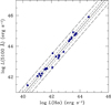 |
Fig. 1. Correlation between the luminosity of the broad Hα emission line and the starlight-corrected AGN continuum luminosity at 5100 Å. Only AGNs with host-galaxy starlight removal from the measured continuum based on HST high-resolution imaging are shown (Bentz et al. 2013), i.e. the AGNs listed in Table 1. The solid line represents the best fit to Eq. (2), with parameters given in line 1 of Table 1. The short-dash lines show the ±1σ envelope, and the long-dash lines show the ±2.6σ (99% confidence level) envelope. |
Radius–luminosity, luminosity–luminosity, and line-width relations: y = a + b(x − x0).
Reverberation-based black-hole masses (Eq. (1)) are based on the measured lag τ of the emission-line flux variations relative to those of the continuum. Estimates of black-hole masses based on individual spectra – ‘single epoch’ (SE) masses – are enabled by the well-known correlation between BLR radius R = cτ and AGN luminosity (Kaspi et al. 2000, 2005; Bentz et al. 2006, 2009a, 2013, and additional historical references in Paper I). Figure 2 shows the relationship between the Hα lag and luminosity based on the data presented in Tables A.1 and B.1. The best-fit parameters to these data are given in line 2 of Table 1; the slope of the relationship is nearly exactly the canonical value b = 0.5. This fundamentally establishes justification for seeking a SE predictor based on the Hα line.
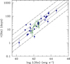 |
Fig. 2. Time-delayed response of the broad Hα line as as a function of Hα luminosity. Since the response time is directly related to the BLR radius by R = cτ, this is known as the R–L relationship. Blue circles are from the RM database (Table A.1) and green triangles are from SDSS-RM (Table B.1). The solid line shows the best fit to Eq. (2), with parameters given in the second line of Table 1. The short- and long-dashed line show the ±1σ and ±2.6σ envelopes, respectively. |
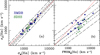 |
Fig. 3. Relationships between line-width measures. (a) Relationship between the Hα line dispersion in the RMS spectrum, σR(Hα), and the mean spectrum, σM(Hα). (b) Relationship between the Hα line dispersion in the RMS spectrum, σR(Hα), and the FWHM in the mean spectrum, FWHMM(Hα). Blue points are from Table 1, (the reverberation mapping database or RMDB sample), green are from Table 2 (SDSS-RM sample). The solid lines are the best fit to Eq. (2) with coefficients from Table 1. The short- and long-dashed lines indicate the ±1σ and ±2.6σ envelopes. The dotted red lines indicate where the two measures are equal. |
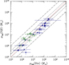 |
Fig. 4. Comparison between virial products based on the Hα data presented in Tables A.1 (blue circles) and B.1 (green triangles) and the virial products based on Hβ in Paper I. The dashed red line shows the locus where the two values are equal. The solid black line shows the best fit to the data. The short- and long-dashed lines show the ±1σ and ±2.6σ envelopes, respectively. The largest outlier is Mrk 202, which Bentz et al. (2010) flag as having an especially dubious Hα lag measurement. |
The other parameter needed to compute a reverberation-based mass is the emission-line width ΔV (Eq. (1)). Broad emission lines typically comprise multiple components, and the line width measured used in Eq. (1) should be based only on the emission-line components that are responding to the continuum variations. To isolate the variable part of the emission line, a root-mean-square residual spectrum (for brevity hereafter referred to as the ‘RMS spectrum’) is constructed. The mean spectrum is defined by
 (8)
(8)
where Fi(λ) is flux of the ith spectrum of the time series at wavelength λ and N is the total number of spectra. The RMS spectrum is then defined by
![Mathematical equation: $$ \begin{aligned} \sigma _{\rm rms}(\lambda ) = \left\{ \frac{1}{N-1} \sum ^N_{1} \left[ F_i(\lambda ) - \overline{F}(\lambda ) \right]^2 \right\} ^{1/2}. \end{aligned} $$](/articles/aa/full_html/2025/04/aa52746-24/aa52746-24-eq9.gif) (9)
(9)
There are multiple parameters that might be used to characterize the emission-line width. Most commonly used are the full width at half maximum (FWHM) and the line dispersion, defined by
![Mathematical equation: $$ \begin{aligned} \sigma _{\rm line} =\left[ \frac{\int (\lambda - \lambda _0)^2 P(\lambda )\,\mathrm{d}\lambda }{\int P(\lambda )\,\mathrm{d}\lambda } \right]^{1/2}, \end{aligned} $$](/articles/aa/full_html/2025/04/aa52746-24/aa52746-24-eq10.gif) (10)
(10)
where P(λ) is the line profile and λ0 is the line centroid
 (11)
(11)
Paper I presents detailed arguments that the line dispersion in the RMS spectrum σR is better than FWHM in the RMS spectrum, FWHMR for computing reverberation masses. We also have carried out a preliminary investigation of other line-width measures and found that there are other good proxies for σR (Dalla Bontà & Peterson 2022), but this discussion is beyond the scope of the current work and will be pursued elsewhere. The aim here is then to determine, given a single spectrum, what line-width measure in the mean or a single spectrum (since the mean spectrum is a reasonable representation of a SE spectrum in the time series) is the better proxy for σR. Figure 3a shows the relationship between σR and the line dispersion in the mean spectrum, σM. Figure 3b shows the relationship between σR and FWHM in the mean spectrum, FWHMM. Best-fit relationships between pairs of parameters are given in third and fourth lines of Table 1. As is the case with Hβ as described in Paper I, σM is an excellent proxy for σR. On the other hand, FWHMM can also be used as a proxy for σR, but the relationship is not close to linear and the additional uncertainty introduced (εy) is more than twice as large as that introduced by σM.
At this point, we compared the virial products obtained with the Hα data in Tables A.1 and B.1 with the Hβ-based virial products we obtained in Paper I (see Fig. 4). For individual sources, in most cases the two virial products agree to within the uncertainties. A simple fit to this distribution, with resulting coefficients shown in line 5 of Table 1, confirms that the slope is less than unity and that the Hα-based virial product sightly exceeds the Hβ-based values with increasing mass. In the analysis that follows, we used the Hβ-based masses as our reference because the typical uncertainties (∼0.113 dex) are considerably smaller than those associated with the Hα-based masses (∼0.358 dex).
3.2. Fits and corrections
The correlations identified above justify a search for a SE formula to estimate black-hole masses from Hα. As a first approximation, we began by trying to reproduce the Hβ RM virial product with the expectation that the BLR radius can be determined from the luminosity and that the line width in the mean spectrum can be used as a proxy for σR. The following equations were used:
![Mathematical equation: $$ \begin{aligned} \log \mu _{\rm RM}(\mathrm{H}\beta )&= a + b\left[ \log L(\mathrm{H}\alpha ) - x_0\right] \nonumber \\&\quad + c\left[\log \sigma _{\rm M}(\mathrm{H}\alpha ) - { y}_0\right] \end{aligned} $$](/articles/aa/full_html/2025/04/aa52746-24/aa52746-24-eq12.gif) (12)
(12)
and
![Mathematical equation: $$ \begin{aligned} \log \mu _{\rm RM}(\mathrm{H}\beta )&= a + b\left[ \log L(\mathrm{H}\alpha ) - x_0\right] \nonumber \\&\quad + c\left[\log \mathrm{FWHM}_{\rm M}(\mathrm{H}\alpha ) - { y}_0\right]. \end{aligned} $$](/articles/aa/full_html/2025/04/aa52746-24/aa52746-24-eq13.gif) (13)
(13)
The best fits to these equations are given in Table C.1. These can be used to produce initial SE predictors:
![Mathematical equation: $$ \begin{aligned} \log \mu _{\rm SE}(\mathrm{H}\alpha )&= 6.996 + 0.501\left[\log L(\mathrm{H}\alpha ) -42.267\right] \nonumber \\&\quad + 2.397\left[\log \sigma _{\rm M}(\mathrm{H}\alpha ) - 3.227\right] \end{aligned} $$](/articles/aa/full_html/2025/04/aa52746-24/aa52746-24-eq14.gif) (14)
(14)
and
![Mathematical equation: $$ \begin{aligned} \log \mu _{\rm SE}(\mathrm{H}\alpha )&= 7.082 + 0.583\left[\log L(\mathrm{H}\alpha ) -42.531\right] \nonumber \\&\quad + 1.173\left[\log \mathrm{FWHM}_{\rm M}(\mathrm{H}\alpha ) - 3.314\right]. \end{aligned} $$](/articles/aa/full_html/2025/04/aa52746-24/aa52746-24-eq15.gif) (15)
(15)
These data and their best fits are shown in Fig. 5, Eq. (14) in panel a and Eq. (15) in panel (b). In both cases, the slope b is shallower than unity, indicating that the line luminosity and line width are, by themselves, unable to accurately predict the reverberation measurement μRM. As noted above, in Paper I, we found that the residuals in this relationship were closely correlated with Eddington ratio, which is the ratio of actual mass-accretion rate relative to the maximum or Eddington rate. This finding is in agreement with the conclusions of others who have investigated the R–L relationship (e.g. Du et al. 2016, 2018; Grier et al. 2017b; Du & Wang 2019; Martínez-Aldama et al. 2019; Fonseca Alvarez et al. 2020). In the upper panels of Fig. 6, we show the residuals in the μRM–μSE relationship for Eqs. (14) (panel a) and (15) (panel b). As in Paper I, we computed a correction to the SE mass by fitting the relationship
 (16)
(16)
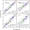 |
Fig. 5. Comparison between SE mass estimates and reverberation measurements. Upper: SE Hα-based virial product predictions using Eqs. (14) and (15) in panels (a) and (b), respectively. The coefficients for the best fit appear in the first two lines of Table 1. Blue circles are data from Table A.1, and green triangles are from Table B.1. The solid line is the best fit to the data, and the dotted red line shows where the measures are equal. The short- and long-dashed lines show the ±1σ and ±2.6σ envelopes, respectively. Lower: Corrected SE masses from Hα-based virial product predictions using Eq. (17) (panel c) and Eq. (19) (panel d), in both cases with log f = 0 arbitrarily. |
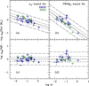 |
Fig. 6. Mass residuals as a function of Eddington rate. (a) Mass residuals (Eq. (16)), i.e. the difference between the measured reverberation virial products and those predicted by Eq. (12). The residuals are plotted vs the Eddington ratio. The solid line represents the best fit, the short-dashed lines the ±1σ envelope, and the long-dashed line the ±2.6σ envelope. Blue circles are from Table A.1, and green triangles are from Table B.1. (b) Mass residuals, i.e. the difference between the measured reverberation virial products and those predicted by Eq. (15). Panels (c) and (d) show residuals after subtraction of the best-fit relations shown in panels (a) and (b). |
Initial, residual, and final fits: y = a + b(x − x0).
Our assumptions and calculations of the Eddington ratio, the most important assumption being our use of the bolometric correction from Netzer (2019), are given in Paper I. The single modification here is that we used Eq. (2) with the relationship shown in Fig. 1 to substitute L(Hα) for  . The reason our correction works is because the simple assumptions we made to compute the Eddington ratio depend only on L(Hα) (or equivalently, LAGN(5100 Å) or L(Hβ)) and μRM, which are known for this sample. The best-fit parameters for Eq. (16) are given in lines 3 and 4 of Table 2. The bottom panels of Fig. 6 show the effect of this correction on the residuals.
Applying the correction of Eq. (16) to the SE masses in the top panels of Fig. 5 yields the corrected SE masses shown in the bottom panels of the same figure. The best-fit parameters for the revised relationship are given in lines 5 and 6 of Table 2 for the case of σM and FWHMM-based masses, respectively. It should be noted that the slopes of these relationships are very close to the expected value of unity, indicating that the three variables identified – line luminosity, line width, and Eddington ratio – are sufficient to estimate the black-hole mass to fairly high accuracy.
4. Formulas for mass estimation
Our initial estimates (Eqs. (14) and (15)) can be combined with the Eddington rate correction (Eq. (16)), which we inverted to solve for an estimate of μRM based solely on L(Hα) and σM(Hα). This yields our equations for the corrected SE virial product estimator, with zero-points adjusted for convenience and for consistency with Paper I,
![Mathematical equation: $$ \begin{aligned} \log M_{\rm SE}&= \log f + 7.413 + 0.554\left[\log L(\mathrm{H}\alpha ) - 42 \right] \nonumber \\&\quad + 2.61\left[\log \sigma _{\rm M}(\mathrm{H}\alpha ) - 3.5 \right], \end{aligned} $$](/articles/aa/full_html/2025/04/aa52746-24/aa52746-24-eq18.gif) (17)
(17)
which has an associated uncertainty
![Mathematical equation: $$ \begin{aligned} \Delta \log M_{\rm SE}&= \left\{ \left( \Delta \log f \right)^2 + \left[ 0.554\, \Delta \log L(\mathrm{H}\alpha ) \right]^2 \right. \nonumber \\&\left. \quad + \left[ 2.61\,\Delta \log \sigma _{\rm M}(\mathrm{H}\alpha ) \right]^2 \right\} ^{1/2}. \end{aligned} $$](/articles/aa/full_html/2025/04/aa52746-24/aa52746-24-eq19.gif) (18)
(18)
We note that the intrinsic scatter, εy = 0.219, needs to be added in quadrature to the formal uncertainty.
Similarly, in the case where FWHM is used as the line-width measure,
![Mathematical equation: $$ \begin{aligned} \log M_{\rm SE}&= \log f + 6.688 + 0.812\left[\log L(\mathrm{H}\alpha ) - 42 \right] \nonumber \\&\quad + 1.634\left[\log \mathrm{FWHM}_{\rm M}(\mathrm{H}\alpha ) - 3.5 \right], \end{aligned} $$](/articles/aa/full_html/2025/04/aa52746-24/aa52746-24-eq20.gif) (19)
(19)
which has an associated uncertainty of
![Mathematical equation: $$ \begin{aligned} \Delta \log M_{\rm SE}&= \left\{ \left( \Delta \log f \right)^2 + \left[ 0.812\, \Delta \log L(\mathrm{H}\alpha ) \right]^2 \right. \nonumber \\&\left. \quad + \left[ 1.634\,\Delta \log \mathrm{FWHM}_{\rm M}(\mathrm{H}\alpha ) \right]^2 \right\} ^{1/2}. \end{aligned} $$](/articles/aa/full_html/2025/04/aa52746-24/aa52746-24-eq21.gif) (20)
(20)
Again, the intrinsic scatter, εy = 0.332, needs to be combined in quadrature with the formal uncertainty.
The mean scale factor is determined by calibrating the virial products μRM to the MBH–σ* relations. Our adopted value, based on the most recent analysis of the largest database, is ⟨log f⟩ = 0.683 ± 0.150 (Batiste et al. 2017). The error on the mean is Δlog f = 0.030 dex and this should also be folded into the mass estimate uncertainty.
5. Discussion
5.1. Limitations
The SE mass predictors developed here and in Paper I include sources in the luminosity range

for the Balmer lines and

for C IV, though the sample size for the latter is very poor below log L(1350 Å) ≈ 42 (e.g. Fig. 9 of Paper I). This does, however, cover most of the known range of AGN activity. The range of Eddington ratio covered by these estimators is
for the Balmer lines with extension to lower rates in C IV, as low as log ṁ ≈ − 3, but with poor sampling. This reaches close to the lowest Eddington ratios expected for broad-line AGNs. Extension to super-Eddington rates (i.e. ṁ > 1) remains to be explored.
Comparison of SE estimates with GRAVITY measurements.
5.2. On the importance of line-width measures
Much of this work has been focused on how the line-width measures are used. In particular, we have argued that if FWHM is used as ΔV in Eq. (1), the mass scale will be erroneously stretched. At larger line widths (higher mass at fixed luminosity), the ratio FWHM/σ is high so that the higher masses are overestimated by using FWHM. Similarly, for narrower lines (lower masses at fixed luminosity) FWHM/σ is low and thus lower masses are consequently underestimated by using FWHM. This point was made very clear by Rafiee & Hall (2011) who demonstrated this for fixed intervals of luminosity. The key point is that the mass scale is stretched at fixed luminosity.
This may obscure the fact that the single most important parameter in AGN black-hole mass estimation is luminosity. This is because the range of luminosity (over four orders of magnitude in the sample discussed here) is much larger than the range of line widths (spanning about a single order of magnitude in this sample). Figure 7 suggests that there is in fact a correlation between luminosity and mass and a crude mass estimate can be made based on luminosity alone, which is tantamount to assuming that the range of Eddington ratio ṁ is very narrow; indeed this realization led to a suggestion that the line width is superfluous and contains little if any additional leverage in estimating AGN black-hole masses (Croom 2011). This is true only if the line-width measurements are very inaccurate (as they sometimes are if they are measured from survey-quality data) or if one is willing to settle for a less than order-of-magnitude mass estimate. More importantly, however, one must be cognizant of the fact that selection effects militate against identification of sources in the upper left and lower right parts of this figure. Luminosity alone is simply not a very good predictor of black-hole mass.
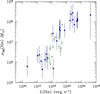 |
Fig. 7. Correlation between the virial product and luminosity of the Hα emission line. The apparent correlation between mass and luminosity is due to selection effects. Sources in the lower right (high luminosity, low mass) are generally excluded by the Eddington limit. Sources in the upper left (low luminosity, high mass) are scarce (a) because high mass objects are rare and therefore mostly at large distances, and thus faint, and (b) because their accretion rates are so low that they do not manifest themselves as AGNs. |
5.3. Comparison with GRAVITY results
As noted earlier, there are a handful of sources that have been spatially resolved with the GRAVITY interferometer and have yielded mass measurements. Here we took luminosity and line-width measures from the published literature and used Eqs. (19) and (40) from Paper I to make comparisons between the GRAVITY measurements and our SE predictors. The results are summarized in Table 3 and shown in Fig. 8. We assumed log f = 0.683.
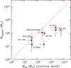 |
Fig. 8. Comparison of the mass predictions from GRAVITY and SE estimates from the current work. Hβ-based SE masses are in black, Hα-based are in red. Note mass rather than the virial product is plotted. |
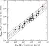 |
Fig. 9. Direct comparison of the mass predictions from Greene & Ho (2005) and from the current work. The dotted red line is the locus where the predictions are equal. The short-dash black lines show this ±1σ envelope and the long-dash lines show the ±2.6σ envelope. Note that mass rather than the virial product is plotted. |
Figure 8 shows that the GRAVITY and SE-based masses are generally consistent at the low-mass end, but not at the high-mass end. In the case of IC 4329A, one SE-based prediction is considerably larger than the other two; this is because the estimate from Li et al. (2024) assumes ∼2 mag of internal extinction of the nucleus. The actual reverberation measurement, using measurements from Li et al. (2024), Eq. (A1) from Paper I, and log f = 0.683) is ∼7.75 in log solar units, closer to the other SE measurements than the estimate based on an internal extinction correction, which suggests that this correction is too large. For the two highest mass sources, 3C 273 and PDS 456, the GRAVITY and SE masses are in poorer agreement, and we note that in both cases, naïve application of the Eddington limits suggests both masses should exceed ∼109 M⊙ (e.g. Nardini et al. 2015). In general, the SE estimates are in better agreement with the RM measurements than the GRAVITY measurements, when they are available.
Fits to comparisons: y = a + b(x − x0).
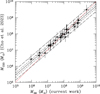 |
Fig. 10. Same as Fig. 10 but for the mass predictions from Cho et al. (2023). |
5.4. Comparison with other single-epoch estimates
Here we compare our Hα-based mass predictions with those previously published. We considered first the early Hα-based mass predictor of Greene & Ho (2005); we rewrote their Eq. (6) as
![Mathematical equation: $$ \begin{aligned} \log M_{\rm GH05}&= 7.331 + 0.55\left[\log L(\mathrm{H}\alpha ) -42\right] \nonumber \\&\quad +2.06\left[\log \mathrm{FWHM(H}\alpha ) -3.5 \right]. \end{aligned} $$](/articles/aa/full_html/2025/04/aa52746-24/aa52746-24-eq30.gif) (21)
(21)
Figure 9 shows a direct comparison of Eqs. (21) and (19) for the sample in Tables A.1 and B.1 (note that we plot the mass rather than the virial product). The best-fit results are given in line 1 of Table 4. Greene & Ho (2005) re-derived the relationship between the Hβ lag and the 5100 Å continuum, and essentially reproduced the result of Kaspi et al. (2005). This was prior to the first recognition that the contaminating starlight needs to be accounted for prior to deriving this relationship (Bentz et al. 2006); consequently the empirical relationship was steeper than the canonical value of 0.5. Empirical relationships among the 5100 Å continuum and the Hα and Hβ emission-line fluxes and between the Hα and Hβ line widths were also used. The scaling factor used was f = 3/4 (Netzer 1990), which was what was widely used prior the first empirical calibration (Onken et al. 2004).
We also compared our results with a more recent effort by Cho et al. (2023), whose database overlaps with ours considerably. Their Eq. (6) can be written as
![Mathematical equation: $$ \begin{aligned} \log M_{\rm C23}&= 7.505 + 0.61\left[\log L(\mathrm{H}\alpha ) -42\right] \nonumber \\&\quad +2.0\left[\log \mathrm{FWHM(H}\alpha ) -3.5 \right]. \end{aligned} $$](/articles/aa/full_html/2025/04/aa52746-24/aa52746-24-eq31.gif) (22)
(22)
The predictions from this equation are compared with those of our Eq. (19) in Fig. 10 (note that we plot the mass rather than virial product). The best-fit parameters are given in line 2 of Table 4. Again, the slope of the relationship between these two predictions is less than unity at least in part because of the lack of an Eddington ratio correction. Moreover, some of the underlying assumptions are so different:
-
Cho et al. (2023) assume a scaling factor value of log f = 0.05 ± 0.12 (Woo et al. 2015) when FWHM is used as the line-width measure. This corrects FWHMM to σM for the mean ratio of ⟨FWHMM/σM⟩ (cf. Collin et al. 2006), but it does not account for the fact that the relationship between FWHMM and σM is neither constant nor linear (e.g. Fig. 9 of Peterson 2014). Indeed, for the Hα lines examined in this investigation the width ratio cover the range
 (23)
(23)compared to the Gaussian value FWHM/σ = 2.35.-pagination
-
The slope we find for the HαR–L relationship, b = 0.497 ± 0.016, is shallower than their slope, b = 0.61 ± 0.04.
-
Cho et al. (2023) assume that the mass scales as FWHM2 while we find that the dependence of mass on FWHM is much shallower for Hα, as it is for Hβ (Paper I).
6. Conclusions
We have derived SE black-hole mass estimators based on the luminosity and line width of the broad Hα emission line (Eqs. (17) and (19)) with a typical formal uncertain of around 0.2–0.4 dex relative to the reverberation masses, depending on which emission-line and line-width measure are used. Both the Hα- and Hβ-based estimators were calibrated over the luminosity range 41 ≲ log LAGN(5100 Å) ≲ 46 erg s−1. Our treatment takes into account the three parameters known to affect black-hole mass: luminosity, line width, and Eddington ratio. As is the case with the Hβ emission line (Paper I), either the line dispersion (Eq. (10)) or the FWHM can be used as the line-width measure, though not interchangeably: the mass dependence on the line width is shallower for the FWHM than for the line dispersion.
Associations between sources in Table A.1 of this paper and Table A1 of Paper I are obvious except in the case of Mrk 6. The three datasets used here were from MJDs 49250–49872, 49980–50777, and 53611–54803.
We note, however, that only 3C 273 = PG 1226+023 and RMID 017 = SBS 1411+533 are flat-spectrum radio quasars; 3C 390.3 is also a radio source, but the jet is inclined to our line of sight.
Acknowledgments
Funding for the Sloan Digital Sky Survey IV has been provided by the Alfred P. Sloan Foundation, the U.S. Department of Energy Office of Science, and the Participating Institutions. SDSS-IV acknowledges support and resources from the Center for High-Performance Computing at the University of Utah. The SDSS web site is www.sdss.org. DG acknowledges the support from PROYECTOS FONDO de ASTRONOMIA ANID – ALMA 2021 Code :ASTRO21-0007. EDB, SC, EMC, and AP acknowledge the support from MIUR grant PRIN 2017 20173ML3WW-001 and Padua University grants DOR 2021-2023; they are also funded by INAF through grant PRIN 2022 C53D23000850006. WNB acknowledges support from NSF grant AST-2407089. LCH was supported by the National Science Foundation of China (11721303, 11991052, 12011540375, 12233001), the National Key R&D Program of China (2022YFF0503401), and the China Manned Space Project (CMS-CSST-2021-A04, CMS-CSST-2021-A06). M.V. gratefully acknowledges financial support from the Independent Research Fund Denmark via grant numbers DFF 8021-00130 and 3103-00146.
References
- Batiste, M., Bentz, M. C., Raimundo, S. I., Vestergaard, M., & Onken, C. A. 2017, ApJ, 838, L10 [CrossRef] [Google Scholar]
- Bentz, M. C., Peterson, B. M., Pogge, R. W., Vestergaard, M., & Onken, C. A. 2006, ApJ, 644, 133 [NASA ADS] [CrossRef] [Google Scholar]
- Bentz, M. C., Peterson, B. M., Netzer, H., Pogge, R. W., & Vestergaard, M. 2009a, ApJ, 697, 160 [Google Scholar]
- Bentz, M. C., Walsh, J. L., Barth, A. J., et al. 2009b, ApJ, 705, 199 [NASA ADS] [CrossRef] [Google Scholar]
- Bentz, M. C., Walsh, J. L., Barth, A. J., et al. 2010, ApJ, 726, 993 [Google Scholar]
- Bentz, M. C., Denney, K. D., Grier, C. J., et al. 2013, ApJ, 767, 149 [Google Scholar]
- Bentz, M. C., Horenstein, D., Bazhaw, C., et al. 2014, ApJ, 796, 8 [NASA ADS] [CrossRef] [Google Scholar]
- Bentz, M. C., Street, R., Onken, C. A., & Valluri, M. 2021, ApJ, 906, 50 [Google Scholar]
- Bentz, M. C., Onken, C. A., Street, R., & Valluri, M. 2023, ApJ, 944, 29 [NASA ADS] [CrossRef] [Google Scholar]
- Blandford, R. D., & McKee, C. F. 1982, ApJ, 255, 419 [Google Scholar]
- Bower, G. A., Green, R. F., Danks, A., et al. 1998, ApJ, 492, L111 [Google Scholar]
- Cappellari, M., Scott, N., Alatalo, K., et al. 2013, MNRAS, 432, 1709 [Google Scholar]
- Carone, T. E., Peterson, B. M., Bechtold, J., et al. 1996, ApJ, 471, 737 [NASA ADS] [CrossRef] [Google Scholar]
- Cho, H., Woo, J.-H., Wang, S., et al. 2023, ApJ, 953, 142 [Google Scholar]
- Clavel, J., Reichert, G. A., Alloin, D., et al. 1991, ApJ, 366, 64 [NASA ADS] [CrossRef] [Google Scholar]
- Collin, S., Kawaguchi, T., Peterson, B. M., & Vestergaard, M. 2006, A&A, 456, 75 [NASA ADS] [CrossRef] [EDP Sciences] [Google Scholar]
- Cretton, N., de Zeeuw, P. T., van der Marel, R. P., et al. 1999, ApJS, 124, 383 [Google Scholar]
- Croom, S. M. 2011, ApJ, 736, 161 [Google Scholar]
- Dalla Bontà, E., & Peterson, B. M. 2022, Astronomische Nachrichten, 343 [Google Scholar]
- Dalla Bontà, E., Ferrarese, L., Corsini, E. M., et al. 2009, ApJ, 690, 537 [Google Scholar]
- Dalla Bontà, E., Davies, R. L., Houghton, R. C. W., et al. 2018, MNRAS, 474, 339 [Google Scholar]
- Dalla Bontà, E., Peterson, B. M., Bentz, M. C., et al. 2020, ApJ, 903, 112 [CrossRef] [Google Scholar]
- Davies, R. I., Tacking, L. J., & Genzel, R. 2004a, ApJ, 602, 148 [NASA ADS] [CrossRef] [Google Scholar]
- Davies, R. I., Tacconi, L. J., & Genzel, R. 2004b, ApJ, 613, 781 [NASA ADS] [CrossRef] [Google Scholar]
- Davis, T. A., Bureau, M., Cappellari, M., et al. 2013, Nature, 494, 328 [NASA ADS] [CrossRef] [Google Scholar]
- de Francesco, G., Capetti, A., & Marconi, A. 2008, A&A, 479, 355 [Google Scholar]
- Dietrich, M., Kollatschny, W., Peterson, B. M., et al. 1993, ApJ, 408, 416 [NASA ADS] [CrossRef] [Google Scholar]
- Dietrich, M., Peterson, B. M., Grier, C. J., et al. 2012, ApJ, 757, 53 [NASA ADS] [CrossRef] [Google Scholar]
- Doroshenko, V. T., Sergeev, S. G., Klimanov, S. A., Pronik, V. I., & Efimov, Y. S. 2012, MNRAS, 426, 416 [NASA ADS] [CrossRef] [Google Scholar]
- Du, P., & Wang, J.-M. 2019, ApJ, 886, 42 [NASA ADS] [CrossRef] [Google Scholar]
- Du, P., Lu, K.-X., Zhang, Z.-X., et al. 2016, ApJ, 825, 126 [CrossRef] [Google Scholar]
- Du, P., Zhang, Z.-X., Wang, K., et al. 2018, ApJ, 856, 6 [NASA ADS] [CrossRef] [Google Scholar]
- Edelson, R., Peterson, B. M., Gelbord, J., et al. 2024, ApJ, 973, 152 [Google Scholar]
- Ferrarese, L., & Merritt, D. 2000, ApJ, 539, L9 [Google Scholar]
- Ferrarese, L., Pogge, R. W., Peterson, B. M., et al. 2001, ApJ, 555, L79 [NASA ADS] [CrossRef] [Google Scholar]
- Fonseca Alvarez, G., Trump, J. R., Homayouni, Y., et al. 2020, ApJ, 899, 73 [CrossRef] [Google Scholar]
- Gaskell, C. M., & Peterson, B. M. 1987, ApJS, 65, 1 [NASA ADS] [CrossRef] [Google Scholar]
- Gebhardt, K., Bender, R., Bower, G., et al. 2000a, ApJ, 539, L13 [Google Scholar]
- Gebhardt, K., Kormendy, J., Ho, L. C., et al. 2000b, ApJ, 543, L5 [CrossRef] [Google Scholar]
- Gebhardt, K., Richstone, D., Tremaine, S., et al. 2003, ApJ, 583, 92 [Google Scholar]
- GRAVITY Collaboration (Sturm, E., et al.) 2018, Nature, 563, 657 [Google Scholar]
- GRAVITY Collaboration (Amorim, A., et al.) 2020, A&A, 643, A154 [NASA ADS] [CrossRef] [EDP Sciences] [Google Scholar]
- GRAVITY Collaboration (Amorim, A., et al.) 2021a, A&A, 648, A117 [NASA ADS] [CrossRef] [EDP Sciences] [Google Scholar]
- GRAVITY Collaboration (Amorim, A., et al.) 2021b, A&A, 654, A85 [NASA ADS] [CrossRef] [EDP Sciences] [Google Scholar]
- GRAVITY Collaboration (Amorim, A., et al.) 2024, A&A, 684, A167 [NASA ADS] [CrossRef] [EDP Sciences] [Google Scholar]
- Greene, J. E., & Ho, L. C. 2005, ApJ, 630, 122 [NASA ADS] [CrossRef] [Google Scholar]
- Grier, C. J., Martini, P., Watson, L. C., et al. 2013a, ApJ, 773, 90 [CrossRef] [Google Scholar]
- Grier, C. J., Peterson, B. M., Horne, K., et al. 2013b, ApJ, 764, 47 [NASA ADS] [CrossRef] [Google Scholar]
- Grier, C. J., Pancoast, A., Barth, A. J., et al. 2017a, ApJ, 849, 146 [NASA ADS] [CrossRef] [Google Scholar]
- Grier, C. J., Trump, J. R., Shen, Y., et al. 2017b, ApJ, 851, 21 [NASA ADS] [CrossRef] [Google Scholar]
- Hicks, E. K. S., & Malkan, M. A. 2008, ApJS, 174, 31 [NASA ADS] [CrossRef] [Google Scholar]
- Kaspi, S., Smith, P. S., Netzer, H., Maoz, D., Jannuzi, B. T., & Giveon, U. 2000, ApJ, 533, 631 [Google Scholar]
- Kaspi, S., Maoz, D., Netzer, H., Peterson, B. M., Vestergaard, M., & Jannuzi, B. T. 2005, ApJ, 629, 61 [Google Scholar]
- Kollatschny, W., Bischoff, K., Robinson, E. L., Welsh, W. F., & Hill, G. J. 2001, A&A, 379, 125 [NASA ADS] [CrossRef] [EDP Sciences] [Google Scholar]
- Kuo, C. Y., Braatz, J. A., Impellizzeri, C. M. V., et al. 2020, MNRAS, 498, 1609 [NASA ADS] [CrossRef] [Google Scholar]
- Li, Y.-R., Hu, C., Yao, Z.-H., et al. 2024, ApJ, 974, 86 [Google Scholar]
- Macchetto, F., Marconi, A., Axon, D. J., et al. 1997, ApJ, 489, 579 [NASA ADS] [CrossRef] [Google Scholar]
- Martínez-Aldama, M. L., Czerny, B., Kawka, D., et al. 2019, ApJ, 883, 170 [CrossRef] [Google Scholar]
- Nardini, E., Reeves, J. N., Gofford, J., et al. 2015, Science, 347, 860 [Google Scholar]
- Nelson, C. H., Green, R. F., Bower, G., et al. 2004, ApJ, 615, 652 [NASA ADS] [CrossRef] [Google Scholar]
- Netzer, H. 1990, Active Galactic Nuclei, 57 [Google Scholar]
- Netzer, H. 2019, MNRAS, 488, 5185 [NASA ADS] [CrossRef] [Google Scholar]
- Onken, C. A., Ferrarese, L., Merritt, D., et al. 2004, ApJ, 615, 645 [Google Scholar]
- Osterbrock, D. E. 1977, ApJ, 215, 733 [Google Scholar]
- Pancoast, A., Brewer, B. J., & Treu, T. 2011, ApJ, 730, 139 [NASA ADS] [CrossRef] [Google Scholar]
- Pancoast, A., Brewer, B. J., Treu, T., et al. 2014, MNRAS, 445, 3073 [Google Scholar]
- Pérez, E., Manchado, A., Pottasch, S. R., & García-Lario, P. 1989, A&A, 215, 262 [Google Scholar]
- Peterson, B. M. 1993, PASP, 105, 247 [NASA ADS] [CrossRef] [Google Scholar]
- Peterson, B. M. 2014, Space Sci. Rev., 183, 253 [Google Scholar]
- Peterson, B. M., Wanders, I., Horne, K., et al. 1998, PASP, 110, 660 [Google Scholar]
- Peterson, B. M., Ferrarese, L., Gilbert, K. M., et al. 2004, ApJ, 613, 682 [Google Scholar]
- Rafiee, A., & Hall, P. B. 2011, MNRAS, 415, 2932 [Google Scholar]
- Reichert, G. A., Rodriguez-Pascual, P. M., Alloin, D., et al. 1994, ApJ, 425, 582 [NASA ADS] [CrossRef] [Google Scholar]
- Rousseeuw, P., & van Driessen, K. 2006, Data Min. Knowl. Discovery, 12, 29 [Google Scholar]
- Sergeev, S. G., Pronik, V. I., Sergeeva, E. A., & Malkov, Y. F. 1999, ApJS, 121, 159 [Google Scholar]
- Sharma, S., Bland-Hawthorn, J., Binney, J., et al. 2014, ApJ, 793, 51 [NASA ADS] [CrossRef] [Google Scholar]
- Shen, Y., Brandt, W. N., Dawson, K. S., et al. 2015, ApJS, 216, 4 [Google Scholar]
- Shen, Y., Grier, C. J., Horne, K., et al. 2024, ApJS, 272, 26 [NASA ADS] [CrossRef] [Google Scholar]
- Simpson, C., Ward, M., O’Brien, P., et al. 1999, MNRAS, 303, L23 [NASA ADS] [CrossRef] [Google Scholar]
- Stirpe, G. M., Winge, C., Altieri, B., et al. 1994, ApJ, 425, 609 [NASA ADS] [CrossRef] [Google Scholar]
- Thomas, J., Saglia, R. P., Bender, R., et al. 2004, MNRAS, 353, 391 [NASA ADS] [CrossRef] [Google Scholar]
- Torres, C. A. O., Quast, G. R., Coziol, R., et al. 1997, ApJ, 488, L19 [NASA ADS] [CrossRef] [Google Scholar]
- Valluri, M., Merritt, D., & Emsellem, E. 2004, ApJ, 602, 66 [Google Scholar]
- van der Marel, R. P., Cretton, N., de Zeeuw, P. T., et al. 1998, ApJ, 493, 613 [Google Scholar]
- van den Bosch, R. C. E., Greene, J. E., Braatz, J. A., et al. 2016, ApJ, 819, 11 [CrossRef] [Google Scholar]
- Wagner, J. 2013, A&A, 560, A12 [NASA ADS] [CrossRef] [EDP Sciences] [Google Scholar]
- Walsh, J. L., Minezaki, T., Bentz, M. C., et al. 2009, ApJS., 269, 39 [Google Scholar]
- Wanders, I., van Groningen, E., Alloin, D., et al. 1993, A&A, 269, 39 [NASA ADS] [Google Scholar]
- Wang, S., Shen, Y., Jiang, L., et al. 2019, ApJ, 882, 4 [CrossRef] [Google Scholar]
- Watson, L. C., Martini, P., Dasyra, K. M., et al. 2008, ApJ, 682, L21 [NASA ADS] [CrossRef] [Google Scholar]
- Winge, C., Peterson, B. M., Pastoriza, M. G., et al. 1996, ApJ, 469, 648 [NASA ADS] [CrossRef] [Google Scholar]
- Woo, J.-H., Yoon, Y., Park, S., et al. 2015, ApJ, 801, 38 [NASA ADS] [CrossRef] [Google Scholar]
- Zhang, Z.-X., Du, P., Smith, P. S., et al. 2019, ApJ, 876, 49 [NASA ADS] [CrossRef] [Google Scholar]
Appendix A: Data from the literature
Reverberation mapped AGNs (Hα).
Appendix B: Data from SDSS-RM
Reverberation mapped AGNs (SDSS Hα).
Appendix C: Multivariate relations
Multivariate relations: z = a + b(x − x0)+c(y − y0).
All Tables
Radius–luminosity, luminosity–luminosity, and line-width relations: y = a + b(x − x0).
All Figures
|
Fig. 1. Correlation between the luminosity of the broad Hα emission line and the starlight-corrected AGN continuum luminosity at 5100 Å. Only AGNs with host-galaxy starlight removal from the measured continuum based on HST high-resolution imaging are shown (Bentz et al. 2013), i.e. the AGNs listed in Table 1. The solid line represents the best fit to Eq. (2), with parameters given in line 1 of Table 1. The short-dash lines show the ±1σ envelope, and the long-dash lines show the ±2.6σ (99% confidence level) envelope. |
| In the text | |
|
Fig. 2. Time-delayed response of the broad Hα line as as a function of Hα luminosity. Since the response time is directly related to the BLR radius by R = cτ, this is known as the R–L relationship. Blue circles are from the RM database (Table A.1) and green triangles are from SDSS-RM (Table B.1). The solid line shows the best fit to Eq. (2), with parameters given in the second line of Table 1. The short- and long-dashed line show the ±1σ and ±2.6σ envelopes, respectively. |
| In the text | |
|
Fig. 3. Relationships between line-width measures. (a) Relationship between the Hα line dispersion in the RMS spectrum, σR(Hα), and the mean spectrum, σM(Hα). (b) Relationship between the Hα line dispersion in the RMS spectrum, σR(Hα), and the FWHM in the mean spectrum, FWHMM(Hα). Blue points are from Table 1, (the reverberation mapping database or RMDB sample), green are from Table 2 (SDSS-RM sample). The solid lines are the best fit to Eq. (2) with coefficients from Table 1. The short- and long-dashed lines indicate the ±1σ and ±2.6σ envelopes. The dotted red lines indicate where the two measures are equal. |
| In the text | |
|
Fig. 4. Comparison between virial products based on the Hα data presented in Tables A.1 (blue circles) and B.1 (green triangles) and the virial products based on Hβ in Paper I. The dashed red line shows the locus where the two values are equal. The solid black line shows the best fit to the data. The short- and long-dashed lines show the ±1σ and ±2.6σ envelopes, respectively. The largest outlier is Mrk 202, which Bentz et al. (2010) flag as having an especially dubious Hα lag measurement. |
| In the text | |
|
Fig. 5. Comparison between SE mass estimates and reverberation measurements. Upper: SE Hα-based virial product predictions using Eqs. (14) and (15) in panels (a) and (b), respectively. The coefficients for the best fit appear in the first two lines of Table 1. Blue circles are data from Table A.1, and green triangles are from Table B.1. The solid line is the best fit to the data, and the dotted red line shows where the measures are equal. The short- and long-dashed lines show the ±1σ and ±2.6σ envelopes, respectively. Lower: Corrected SE masses from Hα-based virial product predictions using Eq. (17) (panel c) and Eq. (19) (panel d), in both cases with log f = 0 arbitrarily. |
| In the text | |
|
Fig. 6. Mass residuals as a function of Eddington rate. (a) Mass residuals (Eq. (16)), i.e. the difference between the measured reverberation virial products and those predicted by Eq. (12). The residuals are plotted vs the Eddington ratio. The solid line represents the best fit, the short-dashed lines the ±1σ envelope, and the long-dashed line the ±2.6σ envelope. Blue circles are from Table A.1, and green triangles are from Table B.1. (b) Mass residuals, i.e. the difference between the measured reverberation virial products and those predicted by Eq. (15). Panels (c) and (d) show residuals after subtraction of the best-fit relations shown in panels (a) and (b). |
| In the text | |
|
Fig. 7. Correlation between the virial product and luminosity of the Hα emission line. The apparent correlation between mass and luminosity is due to selection effects. Sources in the lower right (high luminosity, low mass) are generally excluded by the Eddington limit. Sources in the upper left (low luminosity, high mass) are scarce (a) because high mass objects are rare and therefore mostly at large distances, and thus faint, and (b) because their accretion rates are so low that they do not manifest themselves as AGNs. |
| In the text | |
|
Fig. 8. Comparison of the mass predictions from GRAVITY and SE estimates from the current work. Hβ-based SE masses are in black, Hα-based are in red. Note mass rather than the virial product is plotted. |
| In the text | |
|
Fig. 9. Direct comparison of the mass predictions from Greene & Ho (2005) and from the current work. The dotted red line is the locus where the predictions are equal. The short-dash black lines show this ±1σ envelope and the long-dash lines show the ±2.6σ envelope. Note that mass rather than the virial product is plotted. |
| In the text | |
|
Fig. 10. Same as Fig. 10 but for the mass predictions from Cho et al. (2023). |
| In the text | |
Current usage metrics show cumulative count of Article Views (full-text article views including HTML views, PDF and ePub downloads, according to the available data) and Abstracts Views on Vision4Press platform.
Data correspond to usage on the plateform after 2015. The current usage metrics is available 48-96 hours after online publication and is updated daily on week days.
Initial download of the metrics may take a while.