| Issue |
A&A
Volume 696, April 2025
|
|
|---|---|---|
| Article Number | A67 | |
| Number of page(s) | 14 | |
| Section | Galactic structure, stellar clusters and populations | |
| DOI | https://doi.org/10.1051/0004-6361/202452712 | |
| Published online | 04 April 2025 | |
Parallax-based distances to Galactic H II regions: Nearby spiral structure
1
Department of Astronomy, School of Physics and Astronomy, Yunnan University,
Kunming
650091, China
2
School of Physics and Astronomy, Yunnan University,
Kunming,
650091,
PR China
3
National Astronomical Observatories, CAS,
Jia-20 Datun Road, Chaoyang District,
Beijing
100101, PR China
★ Corresponding authors; This email address is being protected from spambots. You need JavaScript enabled to view it.
This email address is being protected from spambots. You need JavaScript enabled to view it.
Received:
23
October
2024
Accepted:
27
February
2025
Abstract
Context. The spiral structure of the Milky Way is not conclusive, even for the disc regions in the solar neighbourhood. In particular, the arm-like structures uncovered from the overdensity maps of evolved stars are inconsistent with the commonly adopted spiral arm models based on young objects.
Aims. We aim to re-examine the arm segments traced by young objects and better understand the nearby spiral structure.
Methods. We identified the exciting stars of 459 H II regions and calculated their parallax-based distances according to the Gaia DR3. Together with other H II regions with spectrophotometric or parallax-based distances in the literature, we used the largest ever sample of 572 H II regions with accurate distances to reveal the features shown in their distributions projected onto the Galactic disc. We then compared the results to the features traced by other young objects (high-mass star-forming region masers, O-type stars, and young open clusters) and evolved stars.
Results. The structures outlined by different kinds of young objects do not exhibit a significant deviation from each other. The distributions of young objects are in agreement with three arm-like features emerging in the overdensity map of evolved stars. In particular, the Local Arm outlined by young objects follows an arm-like feature delineated by evolved stars and probably spirals outwards towards the direction of ℓ ~ 240° in the third Galactic quadrant.
Conclusions. We conclude that the arm segments traced by young objects and evolved stars are consistent with each other, at least in the solar neighbourhood. In particular, the Local Arm delineated by young objects is reinterpreted as an arm segment with a large pitch angle of 25.2° ± 2.0°, whose inner edge is in good agreement with the recently discovered Radcliffe Wave.
Key words: Galaxy: general / Galaxy: kinematics and dynamics / solar neighborhood / Galaxy: structure
© The Authors 2025
 Open Access article, published by EDP Sciences, under the terms of the Creative Commons Attribution License (https://creativecommons.org/licenses/by/4.0), which permits unrestricted use, distribution, and reproduction in any medium, provided the original work is properly cited.
This article is published in open access under the Subscribe to Open model. This email address is being protected from spambots. You need JavaScript enabled to view it. to support open access publication.
1 Introduction
The spiral structure of the Milky Way, its formation, and its evolution are longstanding problems. Although there have been many efforts dedicated to uncovering the truth since the 1950s (e.g. Oort & Muller 1952; Morgan et al. 1953; van de Hulst et al. 1954; Georgelin & Georgelin 1976; Burton & Gordon 1978; Caswell & Haynes 1987; Dame et al. 1987; Russeil 2003; Hou et al. 2009; Reid et al. 2014, 2019; Xu et al. 2021, 2023), the morphology of Galactic spiral arms, their accurate locations, and the kinematic properties remain elusive (see the reviews by e.g. Foster & Cooper 2010; Xu et al. 2018b; Shen & Zheng 2020; Hou 2021). The controversies are not confined to the distant Galactic disc regions but also exist in the solar neighbourhood for the spiral structure traced by more evolved stars and young objects.
In the past decade or so, the nearby spiral structure traced by young objects has been updated with the developments of the Very Long Baseline Interferometry (VLBI) technique (e.g. Xu et al. 2006) and the data releases of the Gaia mission (Gaia Collaboration 2018, 2023b). Different kinds of young objects yield similar results. The distribution of high-mass star-forming region (HMSFR) masers with VLBI parallax measurements has delineated three spiral arm segments (the Perseus Arm, the Local Arm, and the Sagittarius-Carina Arm) within about 5 kpc of the Sun, as well as a few spurs between them (Xu et al. 2013, 2016; Reid et al. 2014, 2019). The arm segments were then confirmed by using a large number of massive O- and/or B-type stars with Gaia astrometric measurements (e.g. Xu et al. 2018a; Chen et al. 2019; Pantaleoni González et al. 2021), and extended to the southern hemisphere based on the all-sky data of the Gaia DR3 (Xu et al. 2021, 2023). The young open clusters (YOCs; e.g. with ages <20 Myr, Hao et al. 2021) are too young to migrate far from their birthplaces. Hence, they are excellent tracers of spiral structure. The distribution of Gaia YOCs (e.g. Cantat-Gaudin et al. 2018; Soubiran et al. 2018; Liu & Pang 2019; Hao et al. 2020; Cantat-Gaudin et al. 2020; Dias et al. 2021; Hao et al. 2022) traces nearby spiral features consistent with that revealed by HMSFR masers and OB stars (e.g. Hao et al. 2021; Joshi & Malhotra 2023). Similar analyses have also been made by using young stellar objects by Kuhn et al. (2021).
However, the situation gets complicated when evolved stars are used to trace the nearby spiral structure. Miyachi et al. (2019) analysed the surface overdensity map of a sample of turn-off stars with typical ages of about 1 Gyr. They found an arm-like overdensity (see the definition in Sect. 4.2) possibly corresponding to the stellar Local Arm, which is close to the Local Arm traced by HMSFRs (Xu et al. 2018a), but with a visible offset in position and a larger pitch angle. Later, Poggio et al. (2021) derived the overdensity maps and displayed three nearby arm segments based on a sample of upper main-sequence stars from Gaia DR3. The geometry of their suggested Perseus Arm and Local Arm differs significantly from that of many previous models based on young objects (e.g. Reid et al. 2019). The Local Arm traced by upper main-sequence stars extends into the third Galactic quadrant towards l ~ 240° as that of Miyachi et al. (2019). A similar result about the stellar Local Arm was obtained by Lin et al. (2022) by using a sample of Red Clump Stars from Gaia DR3, whose typical age is about 2 Gyr. In addition, many efforts have also been made to depict the nearby spiral structure with stars and characterise the dynamic features (e.g. Monguió et al. 2015; Khoperskov et al. 2020; Martinez-Medina et al. 2022; Lemasle et al. 2022; Joshi & Malhotra 2023; Ardèvol et al. 2023; Uppal et al. 2023; Gaia Collaboration 2023a; Denyshchenko et al. 2024; Widmark & Naik 2024; Ge et al. 2024). The different spiral patterns indicated by young objects and evolved stars pose an observational challenge to the scenarios of nearby spiral arms and the formation mechanism.
Therefore, many efforts in observations will be indispensable to enlarge the sample size of young objects and evolved stars with accurate measurements of basic parameters (distances, proper motions, velocities, etc.), which is the cornerstone of building an accurate map of the nearby spiral structure. An accurate map of the spiral arms will be vital to test the possible formation mechanisms (Lin & Shu 1964; Toomre & Toomre 1972; Sellwood & Carlberg 1984) of the Galactic spiral structure. Additionally, a few studies (e.g. Vallée 2014; Hou & Han 2015; Vallée 2022) suggest that the possible offsets are ~100–500 pc near the arm tangent regions; however, such observational tests have not been well extended to other Galactic disc regions. In theory, the spatial offsets between the spiral arms indicated by different age populations arise only within the framework of the quasi-stationary density wave model (e.g. Dobbs & Baba 2014), which also requires further observational constraints.
H II regions, as a type of young object, are ionised gas clouds surrounding massive young stars or star clusters, with a typical electron temperature of Te ~ 8000 K and an electron density of ne ~ 102–104 cm−3 (Lequeux 2005). Only the massive stars with spectral types of B2 or earlier can produce sufficient ultraviolet photons to ionise the surrounding interstellar medium and form Hii regions (Anderson et al. 2014; Armentrout et al. 2021). The typical age of H II regions is only ~10 Myr. As indicators of massive star formation at the present epoch, H II regions have long been used as excellent tracers of the Galactic spiral structure (e.g. Georgelin & Georgelin 1976; Caswell & Haynes 1987; Russeil 2003; Hou et al. 2009). Although more than 7000 H II regions or candidates have been identified (e.g. Armentrout et al. 2021), the distances for most of them have not been determined with high accuracy (Anderson et al. 2014; Hou & Han 2014), which is the main obstacle to better delineating the Galactic spiral structure with H II regions.
Three different ways have been commonly used to determine the distances of H II regions. They are the trigonometric parallax observations towards the associated maser spots (e.g. Xu et al. 2006; Honma et al. 2012; Reid et al. 2014, 2019), the spectra- photometric measurements of the exciting stars (Russeil 2003; Moisés et al. 2011), and the kinematic method (e.g. Hou & Han 2014). The kinematic distances are model dependent and sometimes present considerable uncertainties, relying on the choice of the Galactic rotation curve, the solution of the kinematic distance ambiguity problem, and the possible deviation from the assumed non-circular rotation (Benjamin 2008; Xu et al. 2018b). In comparison, the trigonometric parallax is believed to be the best method, which has provided accurate distances for dozens of Galactic H II regions by identifying the associated HMSFR masers. The spectra-photometric method is not as accurate as trigonometric parallax, but it can generate relatively accurate distances with uncertainties of about 20% for more than 200 H II regions (e.g. Russeil 2003; Moisés et al. 2011; Foster & Brunt 2015).
In the past decade, the number of identified OB stars has increased considerably (e.g. Reed 2003; Skiff 2014; Mohr-Smith et al. 2015; Maíz Apellániz et al. 2016; Mohr-Smith et al. 2017; Liu et al. 2019b), most of which have accurate astrometric measurements by the Gaia mission. This provides a good opportunity to identify the exciting stars and obtain accurate parallax distances for many Galactic H II regions. This kind of work has only been done for 47 H II regions by Méndez-Delgado et al. (2022) using Gaia DR3 to study the gradients of chemical abundances in the Milky Way. A systematic analysis for a large number of H II regions is absent and will be valuable for some studies, such as the abundance gradients in the Milky Way and the chemical evolution (e.g. Wink et al. 1983; Deharveng et al. 2000; Esteban et al. 2005; Rudolph et al. 2006; Quireza et al. 2006; Maciel & Costa 2010; Wenger et al. 2019), the luminosity function of H II regions (e.g. Smith & Kennicutt 1989; Fich et al. 1990; McKee & Williams 1997), and triggered star formation by the expansion of H II regions (e.g. Klessen & Glover 2016; Liu et al. 2015, 2016).
In particular, systematic analysis of a large sample of H II regions with accurate distance measurements facilitate to carry out work that pays attention to the property of the Galactic spiral structure. This work is organised as follows. In Sect. 2, we describe the archived data for H II regions and massive OB stars. The analysis of parallax-based distances to a sample of Galactic H II regions is given in Sect. 3. The results are presented in Sect. 4, including the nearby spiral structure traced by H II regions complemented with other young and evolved objects for comparison. Discussions and conclusions are in Sects. 5 and 6, respectively.
2 Data
2.1 Galactic H II regions
The Wide-field Infrared Survey Explorer (WISE; Wright et al. 2010) catalogue of H II regions (Anderson et al. 2014) is the largest data set of Galactic H II regions and candidates. The catalogue lists about 8400 sources, including their coordinates, radius, recombination line velocity, and/or molecular line velocity, if available from previous literature or the latest observations (e.g. Anderson et al. 2011, 2015; Wenger et al. 2021). These sources were identified according to their mid-infrared morphology. Essentially, all H II regions exhibit a good mid-infrared morphology (Anderson et al. 2014) in WISE observations: The 12 µm emission associated with an H II region primarily originates from polycyclic aromatic hydrocarbon molecules in the photodissociation region, surrounding the extended 22 µm emission. The 22 µm emission is mostly from hot dust, coincident with the ionised gas traced by radio continuum emission (e.g. see Deharveng et al. 2010; Anderson et al. 2011) and/or recombination lines.
The massive young star(s) contributes to the ionising flux of an H II region and, hence, is expected to be close to the midinfrared 22 µm, radio continuum, or recombination line emission peak(s). For many Galactic H II regions, especially those with a radius smaller than 1′, there is a lack of high-quality radio continuum images, partially because most of the existing radio continuum surveys have a resolution larger than about 1′ (e.g. Stil et al. 2006; McClure-Griffiths et al. 2005; Taylor et al. 2003). An even worse situation is found for the available survey dataset of radio recombination lines (e.g. Alves et al. 2015; Liu et al. 2019a; Anderson et al. 2021; Hou et al. 2022). In comparison, the infrared image data of Galactic H II regions always have better angular resolution. For the WISE 22 µm dataset, its resolution (12′′) and sensitivity (6 mJy) make it possible to identify the detailed mid-infrared morphology of many Galactic H II regions. In this work, we identify the central exciting star(s) of WISE H II regions by matching their 22 µm morphology with the known O- and early B-type stars.
2.2 Massive young stars
In the past few decades, there have been considerable efforts to identify Galactic OB stars (e.g. Reed 2003; Mohr-Smith et al. 2015; Maíz Apellániz et al. 2016; Mohr-Smith et al. 2017; Liu et al. 2019b). Skiff (2014) has compiled a catalogue of OB stars from literature, which has been updated until 2022 May 13, and contains 138 604 spectroscopically confirmed OB stars. To our knowledge, it is the largest sample of spectroscopically confirmed OB stars available to date. In addition, Chen et al. (2019) identified 6858 highly confident candidates of O- and early B- type stars by using the photometric data of the VST Photometric Hα Survey (Drew et al. 2014) and the second Gaia data release (Gaia Collaboration 2018). Together with 8022 known O-B2 stars in literature, they built a sample of O- and early B-type stars with robust parallax distances (parallax uncertainties <20%) and also proper motions.
We adopt the catalogues of Skiff (2014) and Chen et al. (2019) as the sample of O-B2 stars to initiate this work. First, we check and solve the redundancy problem for these two catalogues. 755 duplicates are identified based on the specific spectral types as well as the uniqueness of the Gaia DR3 ID, and removed accordingly. Then, we update the parallaxes and proper motions for the O-B2 stars with the Gaia DR3 (Gaia Collaboration 2023b), which has significantly improved the accuracy of parallax measurements, with median parallax uncertainties of 0.02–0.03 mas for the G band magnitude <15, 0.07 mas at G = 17, 0.5 mas at G = 20, and 1.3 mas at G = 21 mag.
3 Distances of Galactic H II regions based on Gaia
3.1 Exciting stars
To identify the exciting stars of H II regions, first of all, we single out the candidates by searching the O-B2 star(s) situated within the angular radius of an H II region. 781 H II regions are selected with 3211 O-B2 stars potentially associated. Then, we inspect each of them by using the SIMBAD database (Wenger et al. 2000), in case some O-B2 stars are not listed in Skiff (2014) and Chen et al. (2019), but given by the SIMBAD. 283 additional O-B2 stars are obtained, which are confirmed spectrally with parallax measurements. We hereto obtain 781 H II regions with 3494 candidate O-B2 stars (also see Table 1).
As mentioned in Anderson et al. (2014), the angular radius of an H II region was determined based on the extent of the 12 µm emission tracing the photodissociation region, which encloses the associated 22 µm mid-infrared emission originating from warm dust within the ionised volume of the H II region. Considering that the 22 µm morphology is generally complex (e.g. see Fig. 1), the boundary of an H II region needs to be described as accurate as possible to count the exciting star(s). First, we extract regions outside the H II region radius and free from bright 22 µm emission. The mean and standard deviation are calculated from these extracted pixels, respectively, as the background value and σ. The H II region boundary is then defined as the 3σ level above the background. Overall, the newly defined boundaries of the H II regions are, as expected, smaller than that determined by Anderson et al. (2014). Accordingly, we exclude O-B2 stars for the related H II regions falling within their radius but outside their boundary. We notice that tens of H II regions show large angular radii (e.g. more than hundreds of arcseconds) with very weak 22 µm emission, they are discarded in this work since their boundaries are difficult to define with high confidence. We have 473 H II regions with 1826 candidate O-B2 stars. Additional 14 H II regions are further discarded as the parallax values of their candidate O-B2 stars are not consistent with each other in the 3σ level. After these steps, we have 459 H II regions with 1592 candidate O-B2 stars (see Step 3 in Table 1). These O-B2 stars have parallax uncertainties at a median value of 4.6%.
It is worth noting that despite our rather strict selection procedures, some of the candidate stars may be foreground or background sources. To alleviate this issue, we required that the parallax values of most stars falling within the boundary of an H II region should be consistent within the 3σ level. For 75 of the 459 H II regions, some candidate stars show a large difference beyond the 3σ level from the major population, and are thus treated as foreground or background stars. Following this standard, about 19.5% of the 1075 candidate stars within these 75 H ii regions are eliminated. The mean radius of these 75 H II regions is ∼829″, larger than that of the 459 H II regions of ∼430″, favouring their possibility of being foreground or background stars.
To sum up briefly, we pick out 459 H II regions with 1382 candidate exciting stars associated (see Step 4 in Table 1). Six exemplar H II regions are shown in Fig. 1. The parallaxes, proper motions, and their uncertainties from Gaia DR3 are given in Table A.1 for the stars, which are used in the following to calculate the H II region distances.
Summary of the number of sources retained at each step.
3.2 Distances to HII regions
Once the exciting star(s) have been identified, the distance of an H II region can be derived from the stellar distance(s). To infer reliable distances for the vast majority of Gaia stars from the parallax measurements, a series of probabilistic methods have been developed (e.g. Bailer-Jones 2015; Astraatmadja & Bailer-Jones 2016a,b; Bailer-Jones et al. 2018; Chen et al. 2019). These methods generally involved a likelihood based on the measurements or the data processing, as well as a prior distribution that describes the space density distribution of stars. Based on Gaia DR3, Bailer-Jones et al. (2021) has estimated two types of distance for 1.47 billion stars, that is, the geometric distance and the photogeometric distance. Both methods adopted a uniform direction-dependent prior that varies smoothly as a function of the Galactic longitude and latitude, considering the colours and magnitudes of the Gaia stars, as well as a zero-point offset for the parallaxes. In particular, the photogeometric distances utilised additional information of the G-band magnitudes and the BP-RP colours of the Gaia stars, which helps improve the precision of distance estimates, especially for the stars in distant Galactic regions and the stars with poor parallax measurements. We cross-matched our sample of exciting stars with the catalogue of Bailer-Jones et al. (2021) to obtain both types of distance. In addition, we considered a distance directly estimated from the inverse parallax for comparison.
Before choosing the most suitable distance estimator, we derive the distances of these H II regions based on the stellar data. For an H II region with only one associated star, the distance and its uncertainty are directly taken from the stellar data. In cases where an H II region has at least two associated stars, we calculated the mean value of stellar distances, which is taken as the H II region distance. Based on the above criteria, the 459 H II regions are divided into three different groups as annotated in Table 2. (1) Group I: the H II region has more than one associated star and all the stars present consistent distances. Therefore, the estimated distances of these 160 H II regions in Group I ought to be reliable. (2) Group II: the H II region originally has two or more associated stars, but only one is left after the above criteria. (3) Group III: the H II region has only one associated star. In total, Groups II and III contain 299 H II regions. We find their mean radius to be ∼290″, 1.5 times less than that of the entire selected H II region sample of ∼430″. We therefore assume that most (if not all) of such H II regions have a good association with the corresponding single candidate star, and thus have a reliable distance determination.
The comparisons of different types of the Hii region distance are shown in Fig. 2. The photogeometric distances are consistent with the geometric ones considering the uncertainties for most H II regions. An outlier G331.172-00.460 is near the Galactic plane; hence the correction for extinction may be insufficient (Bailer-Jones et al. 2021; Méndez-Delgado et al. 2022), resulting in poor reliability of the photogeometric distance. As shown in the right panel of Fig. 2, the distances directly estimated from the inverse parallaxes tend to give larger values than the photogeometric or geometric method, especially for the sources with distances ≳ 3 kpc. In distant Galactic regions, the photogeometric distances typically have smaller uncertainties than the other two methods for most H II regions. Considering the suggestions given by Bailer-Jones et al. (2021) and Gaia Collaboration (2023a), the photogeometric distance is preferentially adopted in this work and listed in Table 2 and Table A.1. In addition, if the photogeometric distance is unavailable or in the case of G331.172-00.460, the distances are replaced with the geometric values and annotated in the Tables.
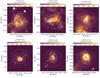 |
Fig. 1 Examples of H II regions with the candidate counterpart(s) of O-B2 stars (white star symbols). The WISE images of the W4 band (22 µm, colour maps) are shown as backgrounds. The contour levels with the corresponding data numbers (white) are marked in each panel, and the first level is adopted to indicate the H II region boundary (see Sect. 3.1). The dashed circle in each plot is the size of the H II region determined from the angular radius parameter given by the WISE H II region catalogue (Anderson et al. 2014). |
H II regions with parallax distances based on Gaia DR3.
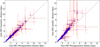 |
Fig. 2 Comparison of the photogeometric distances of the 459 H II regions with the other two types of distance determined from the Gaia DR3. Left: photogeometric distance versus geometric distance. Right: photogeometric distance versus inverse parallax. The grey line in each panel represents the equal line. The grey dashed ellipse denotes the H II region G331.172-00.460 (see Sect. 3.2). |
3.3 Comparison with previous results
Part of the 459 H II regions also have determined distances in literature, either by the trigonometric parallax method, the spectra-photometric measurements, or by the kinematic method. We compare the derived parallax-based distances in this work with the reference results.
The HMSFR masers with trigonometric parallax measurements are collected from the literature (e.g. Reid et al. 2019; VERA Collaboration 2020; Xu et al. 2023; Bian et al. 2024, and references therein) and cross-matched with the 459 H II regions. 29 HMSFR masers are falling within the H II regions defined by the angular radii (Anderson et al. 2014). After an inspection of the mid-infrared images of the H II regions, five HMSFR masers were excluded because they are located outside the H II region boundaries (see Sect. 3.1). Then, the distances of the remaining 24 H II regions (see red dots in Fig. 3) are calculated according to the parallax data of the associated HMSFR masers. As shown in Fig. 3, the results are in agreement with the parallax-based distances adopted in our work. Meanwhile, Méndez-Delgado et al. (2022) has estimated the distances for 47 H II regions by employing a method of identifying the ionising or associated stars located within the boundaries of H II regions based on Gaia DR3. The geometric distance of Gaia Early Data Release 3 or the kinematic distances of Wenger et al. (2019) are adopted to represent the distances for their sample. Additionally, their procedures and criteria for identifying the associations are not the same as in this work. We cross-matched our sample with their results and found that there are 34 H II regions overlapped. A comparison of their distance values (see blue dots in Fig. 3) with our results is presented in Fig. 3, which also demonstrates consistency for most of the targets.
The spectra-photometric method is not as accurate as the trigonometric parallax method but is still capable of providing relatively accurate distances. We collected the H II regions with spectrophotometric distances determined in previous works (Russeil 2003; Russeil et al. 2007; Moisés et al. 2011; Foster & Brunt 2015), and cross-matched the sample with our results. Fig. 4 presents a comparison between the spectrophotometric distances and our results for the 104 matched H II regions. For most of the H II regions with distances ≲4 kpc, these two methods give consistent results, although the spectrophotometric distances typically have larger uncertainties. But in distant regions (e.g. ≳4 kpc), these two distances tend to have larger deviations for most sources, which is probably related to the uncertainties on the Galactic extinction models.
At present, most of the known H II regions only have kinematic distances, which sometimes present large uncertainties. With the information from the aforementioned literature, as well as the catalogues of Wenger et al. (2021) and Liu et al. (2019a), we collect the radial velocities VLSR in the frame of the Local Standard of Rest (LSR) for 267 of 459 H II regions. These velocities were obtained by observing the ionised gas using radio recombination lines, optical Hα line, and transitions from different molecular species (e.g.12CO, 13CO, CS, and NH3). Then, the kinematic distances of these H II regions are re-calculated according to the Galactic rotation model of Reid et al. (2019) with the tool developed by Wenger et al. (2018), which involved a Monte Carlo technique to account for the distance uncertainties. If the kinematic distance ambiguity problem has not been resolved for an H II region in literature (e.g. Anderson et al. 2014), we adopted the one closer to the parallax distance (see Wenger et al. 2018, for detail). In addition, since the estimated kinematic distances will have large uncertainties for the sources around the Galactic Centre (GC) and Galactic anti-centre directions, we removed the H II regions located within the zones of −15° < ℓ < 15° and 160° < ℓ < 200° as suggested by Wenger et al. (2018). Finally, we obtain kinematic distances for 184 H II regions in our sample. The line velocities and the calculated kinematic distances are listed in Table 2. The comparison between the parallax-based distances (dp) and the calculated kinematic distances (dkin) is shown in Fig. 5. The kinematic distances typically have larger uncertainties for the sources with d⊙ <4 kpc. After an inspection of the fractional difference |dkin − dp |/dp, we find that the mean and median values are 0.50 and 0.24, respectively. These results are similar to that of Wenger et al. (2018, see their Table 4), who has shown that the mean and median absolute fractional differences between the kinematic and parallax distances are 36% and 26%, respectively. In this work, 24 of the 184 H II regions have differences |dkin − dp| larger than 2 kpc. In addition, the kinematic method tends to give larger distance values for many H II regions by a mean factor of ∼1.5, comparable to the finding of Reid et al. (2009) and Jing et al. (2023). As shown in the lower panel Fig. 5, accurate distances of H II regions are crucial for building a reliable map of the nearby spiral arms.
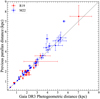 |
Fig. 3 Comparison between the parallax-based distances of H II regions given by this work and the reference values. The red dots indicate the sources with estimated distances from the associated HMSFR masers primarily from Reid et al. (2019). The blue dots are the H II regions from Méndez-Delgado et al. (2022), whose distances are based on Gaia DR3. The grey line represents the equal line. Abbreviations for the references are: R19, Reid et al. (2019); M22, Méndez-Delgado et al. (2022). |
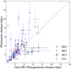 |
Fig. 4 Comparison between the parallax-based distances of H II regions given by this work and the spectrophotometric distances obtained from previous works. Abbreviations for the references are R03, Russeil (2003); R07, Russeil et al. (2007); M11, Moisés et al. (2011); F15, Foster & Brunt (2015). The dashed grey line represents the equal line. |
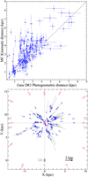 |
Fig. 5 Upper: comparison between the parallax-based distances of H II regions given by this work and the kinematic distances. The grey line is the equal line. Lower: distributions of the H II regions projected onto the Galactic disc, to better show the influence of updated distance parameters on the delineated spiral arm segments. The starting point and ending point of each arrow represent the positions of an H II region according to the kinematic distance and the parallax-based distance, respectively. The locations of H II regions based on the parallax distances are marked with blue dots. In the plot, the Sun is at (0, 8.15) kpc (Reid et al. 2019), while the Galactic Centre is at (0.0, 0.0) kpc. Q1–Q4 indicate the four Galactic quadrants. |
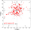 |
Fig. 6 Distributions of 572 H II regions (Sect. 4.1) with accurate distances projected onto the Galactic disc. The H II regions with parallax-based (P) distances are shown by red dots, while those with spectrophotometric (S) distances are indicated by grey dots. Also shown in the plot are the distance uncertainties (underlying line segments). The dot size is proportional to the estimated radio luminosity of the H II region at 5 GHz. The positions of the Sun and GC are the same as the lower panel of Fig. 5. |
4 Spiral structure in the solar neighbourhood
4.1 H II region distribution and comparison to other young objects
To better reveal the spiral structure in the solar neighbourhood traced by H II regions, the sample size of Galactic H II regions having accurate distances should be as large as possible. Therefore, besides the 459 H II regions given by this work, we additionally collect 12 H II regions having parallaxbased distances (Méndez-Delgado et al. 2022), and the other 101 H II regions with available spectrophotometric distances (Russeil 2003; Russeil et al. 2007; Moisés et al. 2011; Foster & Brunt 2015). We note that 20 of 101 H II regions have spectrophotometric distances > 4 kpc, which are considered with large uncertainties, as shown in Fig. 4, and thus should be treated with caution. Fig. 6 presents the projected distributions of the 572 H II regions on the Galactic plane. The radio luminosity of the H II regions at 5 GHz used for weighting the symbol sizes (e.g. Georgelin & Georgelin 1976; Hou & Han 2014) are derived according to the relation between radio luminosity and physical diameters given by Paladini et al. (2004).
As shown in Fig. 6, the distribution of H II regions presents complex structures, including some cavities and overcrowded regions. Although the number and exact position of spiral arms are still open questions (Foster & Cooper 2010; Xu et al. 2018b, 2023), the overcrowded regions can be related to the segments of spiral arms referring to the commonly adopted models of Galactic spiral structure (e.g. see Reid et al. 2019; Xu et al. 2023). They are the Scutum-Centaurus Arm, the Sagittarius- Carina Arm, the Local Arm, the Perseus Arm, and the Outer Arm from the inner to the outer Galactic disc. Besides the major spiral arm segments, some features traced by H II regions are coincident with spur or spur-like structures reported in previous works, including the spur near the direction of ℓ ~ 50° (Xu et al. 2016), the Cepheus spur which starts from the Local Arm (X ~ 1 kpc, Y ~ 8.15 kpc) and ends at the Perseus Arm around ℓ ~ 210° (Pantaleoni González et al. 2021), and a spur-like structure bridging the Scutum Arm and the Sagittarius Arm (Reid et al. 2019) etc. In addition, the structure extending from (X ~ 1.5 kpc, Y ~ 8 kpc) to the direction of ℓ ~ 235° is well aligned with the so-called Radcliffe Wave, which was first discovered as a sinusoidal vertical feature of dense molecular gas (Alves et al. 2020).
To confirm the features shown in the distribution of H II regions, the HMSFR masers, O-type stars, and YOCs (ages < 20 Myr) with lifetimes comparable to or even younger than H II regions are collected from references to make a comparison. The HMSFR masers are taken from the literature discussed in Section 3.2. In addition to the 1090 spectroscopy-confirmed O-type stars from Xu et al. (2021), the extra 592 O-type stars are obtained from the updated catalogue of Skiff (2014). The redundancy of these O stars with those used to calculate the H II region distances has been checked and removed. The sample of 633 YOCs is derived from Hao et al. (2021). All of these YOCs have accurately determined distances based on the parallax measurements of a large number of member stars by the Gaia Early Data Release 3. The distributions of these young objects together with H II regions are given in Fig. 7. As shown in the plots, the structures traced by H II regions share consistent aggregation areas indicated by HMSFR masers, O-type stars, and YOCs. On the other hand, some cavities appearing in the H II region map are replenished by O-type stars and YOCs. For instance, the apparent gap identified in the Carina Arm (ℓ ~ 320°) is not genuine due to the limitation of the sample size of our H II regions, and this zone is enriched with some O-type stars and YOCs. The occurrence in the Perseus Arm (ℓ ~ 150°) may be a real cavity structure, which also appears in the results of Xu et al. (2023) and Gaia Collaboration (2023a). Overall, the structures outlined by young objects with parallax-based distances do not exhibit a significant deviation from each other. Moreover, the results also suggest that the influence of foreground or background stars for the 299 H II regions with a single candidate star (see Sect. 3.1) ought to be inapparent for mapping the nearby spiral structure.
How to derive a true picture of the Galactic spiral structure from the distributions of young objects is a problem. The commonly adopted model of the Galactic spiral structure has been challenged by observations (e.g. see Xu et al. 2023). If we do not have prior knowledge about the overall spiral structure of the Milky Way, the relation of the overcrowded regions to the nearby spiral arms is not easily discernible from Figs. 6 and 7. Some factors complicate the attempts to get an uncontroversial picture. The formation of massive stars is not confined to the major spiral arms but also occurs in the arm branches, arm spurs, and feathers as observed in spiral galaxies (e.g. Elmegreen 1980). Additionally, the formation sites of young objects are always scattered and/or clumped in spiral arms, resulting in patchy or bifurcate appearance of arm-like features. In contrast, the influence of these factors is not so serious for the widely distributed evolved stars, which dominate the mass of visible matter in the Galactic disc. Therefore, it will be beneficial to compare the distribution of young objects with more evolved stars to reveal the nearby spiral structure better.
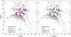 |
Fig. 7 Distributions of H II regions overlaid with HMSFR masers (open triangles), O-type stars (blue dots, left panel), and YOCs (cyan dots, right panel). An equal size of the symbol is adopted for masers and O-type stars. The dot size for each YOC is proportional to the number of member stars as Hao et al. (2021). The H II regions and the positions of the Sun and GC are the same as Fig. 6. |
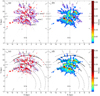 |
Fig. 8 Top two panels: spatial distribution of H II regions (a), and the density map of young objects (b). The contours in panels (a), (b), and (c) represent the overdensity map of upper main-sequence stars (Poggio et al. 2021). The contour levels are 0 for the dashed line, as well as 0.2 and 0.4 for solid lines. Additionally, three arm-like features identified by Poggio et al. (2021) are labelled in panel (a) as arm-1, arm-2, and arm-3 from the inner to the outer Galactic disc. Bottom two panels: similar to the upper panels, but the results are overplotted on the spiral arm models of Xu et al. (2023, black solid lines) and Reid et al. (2019, grey dashed lines). The arm segments are the Outer Arm, the Perseus Arm, the Local Arm, the Carina/Sagittarius-Carina Arm, and the Scutum Arm from the outer to the inner Galactic disc. |
4.2 Comparison with more evolved stars
In this work, the overdensity map of upper main-sequence stars provided by Poggio et al. (2021) is adopted for indicating the distribution of evolved stars for comparison. As mentioned in Sect. 1, different works for example by using turn-off stars (Miyachi et al. 2019), upper main-sequence stars (Poggio et al. 2021), Red Clump Stars (Lin et al. 2022), and B3 to B9 stars (Ge et al. 2024) have given consistent results about the overdensity map of stars in the solar neighbourhood. In the following, we name the three arm-like features shown in the overdensity map of upper main-sequence stars as arm-1, arm-2, and arm-3 from the inner to the outer Galactic disc (see Fig. 8) since their correspondence to the major spiral arms is still inconclusive.
Following the method of calculating the dimensionless stellar density (e.g. Poggio et al. 2021; Lin et al. 2022), the local density for the position (X, Y) of young objects (H II regions, HMSFR masers, O-type stars, and YOCs) can be expressed as
![Mathematical equation: $\Sigma (X,Y) = {1 \over {N{h^2}}}\sum\limits_{i = 1}^N {\left[ {K\left( {{{X - {x_i}} \over h}} \right)K\left( {{{Y - {y_i}} \over h}} \right)} \right]} ,$](/articles/aa/full_html/2025/04/aa52712-24/aa52712-24-eq17.png) (1)
(1)
where
 (2)
(2)
Here, K is the Epanechnikov kernel function, and h stands for the kernel bandwidth (taken as 0.3 kpc), (xi, yi) is the position for the ith young object and N is the total number. The results are given in panels (a) and (b) of Fig. 8.
As shown in Fig. 8, both the distributions of H II regions and the density map of young objects are in good agreement with the three arm-like features appearing in the overdensity map of upper main-sequence stars. The results indicate that the spiral structures traced by young objects and evolved stars are probably consistent with each other, at least in the solar neighbourhood. Based on panels (a) and (b) of Fig. 8, the outer part of arm-1 is well consistent with the Sagittarius-Carina Arm defined by Reid et al. (2019) and Xu et al. (2023), the arm-2 overlaps with their Local Arm in the first and second Galactic quadrants but appears to be an outward feature towards the direction of ℓ ~ 240° in the third Galactic quadrant, the arm-3 starts from the second Galactic quadrant and spirals outwards with a large pitch angle (Levine et al. 2006). The cavity structure around (X, Y) ~ (1, 10) kpc is interpreted as inner arm regions rather than a gap in the Perseus Arm defined by previous works. This picture conflicts with the commonly adopted models of the Galactic spiral arms.
The spiral arm models given by previous works (e.g. Reid et al. 2019) for the combination of various young objects can explain the features shown in Figs. 6 and 7 (also see the lower two panels of Fig. 8), but deviate as large as more than 1 kpc from the two arm-like structures (arm-2 and arm-3) appearing in the overdensity map of evolved stars, which dominate the mass of visible matter in the Galactic disc. These results imply that some modifications to these commonly used models are necessary given the following considerations:
(1) The spiral structures traced by young objects and evolved stars should not present large offsets in positions in the solar neighbourhood. The possible offsets between the spiral arms traced by young objects and old stars are about ~100–500 pc at the spiral arm tangents of the Milky Way (e.g. Hou & Han 2015; Vallée 2022), which should be larger than that in the regions close to the co-rotation radius if the (quasi-stationary) density wave theory (Lin & Shu 1964, 1966; Shu 2016) applies to the Milky Way Galaxy (Roberts 1969; Foyle et al. 2011). The solar neighbourhood is just around the Galactic co-rotation radius (~8.5 kpc, e.g. Dias et al. 2019). In addition, based on the observations towards external spiral galaxies, Yu & Ho (2018) also suggest that the possible offsets between the two different types of spiral arms are generally small, particularly in regions near the co-rotation radius of galaxies. Except for the (quasi-stationary) density wave theory, the mechanisms for the spiral formation do not predict the offset between the spiral arms traced by young objects and evolved stars (e.g. Dobbs & Baba 2014).
(2) In the models of Hou & Han (2014), Reid et al. (2019) and Xu et al. (2023), the Local Arm is extended to the direction of ℓ ~ 260° (see Fig. 8) as there are clumps of young objects around (X, Y) ~ (−2, 8.2) kpc. A recent study (Ge et al. 2024) have shown that they are probably transient and younger structures compared to the three arm-like features shown in Fig. 8. Ge et al. (2024) find that these clumps are only prominent in the distributions of O-B2 stars, and gradually become invisible when B3–B5, B6–B7, B8, and B9 stars are used to create the overdensity maps. In contrast, the three arm-like features are still visible.
Based on the above considerations, we fit the arm-2 segment traced by H II regions using a commonly used logarithmic spiral model, defined as
 (3)
(3)
where R and β are the Galactocentric radius and azimuth angle, respectively. Here, β is defined as 0° from the Galactic Centre towards the Sun and increases with Galactic rotation. ψ is a pitch angle with a reference Galactocentric radius Rref and azimuth angle βref. We obtain the best-fitted results with (Rref, βref) = (9.6±0.l kpc, −7.0° ± 1.4°) and ψ = 25.2°±2.0°, as shown in Fig. 9. The line tracing the centre of the arm-like feature spirals outwards towards the direction of ℓ ~240° over 6 kpc in length in the third quadrant. The pitch angle of arm-2 is larger than that of the Local Arm given by previous works (e.g. ~ 9° – 16°, Reid et al. 2019; Miyachi et al. 2019; Hao et al. 2021; Lin et al. 2022; Xu et al. 2023), but match the distributions of H II regions, other young objects and the overdensity map of evolved stars. Although the sample size is small for the third Galactic quadrant region, the arm-3 outlined by distant H II regions generally follows the Perseus Arm given by Levine et al. (2006) based on the distribution of H I gas, which has a pitch angle of 24° and is directly adopted in this work. Since arm-1 shows excellent consistency in both young objects and evolved stars, the Sagittarius-Carina Arms modelled by Reid et al. (2019) and Xu et al. (2023) are directly adopted and shown in the plot.
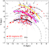 |
Fig. 9 Distributions of H II regions overlaid with the corresponding spiral arm models. The fuchsia solid line traces the best-fitted Local Arm given by this work (see Section 4.2). The yellow curved line presents the Perseus Arm determined from the perturbed surface density map of H I by Levine et al. (2006). The solid and long-dashed curved lines in the plot indicate the best-fitted Carina/Sagittarius-Carina Arm (thick) and the other arm segments (thin) given by Xu et al. (2023) and Reid et al. (2019), respectively. H II regions and the positions of the Sun and GC are the same as Fig. 6. The overdensity map of evolved stars (blue) is also shown in the plot to make a comparison. |
5 Discussions
5.1 Evolved understanding to the Local Arm
In this work, it is shown that the Local Arm traced by young objects is consistent with the overdensity distribution of evolved stars, and probably spirals outwards towards the direction of ℓ ~ 240° in the third Galactic quadrant, rather than towards ℓ ~ 260°. This view is not consistent with the commonly adopted spiral arm models but has been proposed in some references.
Early studies (Morgan et al. 1953; Becker & Fenkart 1963; Becker 1964; Courtès et al. 1970) have indicated the presence of three nearby spiral arms (i.e. see their Fig. 1), which were suggested to be the Perseus Arm, the Orion Arm (also named as the Local Arm, the Orion-Cygnus Arm), and the Sagittarius Arm. The Local Arm was taken as one of the three spiral arm segments in the solar neighbourhood, having a large pitch angle of ~20° (e.g. Avedisova 1985) and extending towards ℓ ~ 240° (e.g. Moffat et al. 1979).
Georgelin & Georgelin (1976) gave a weighted distribution of H II regions in the Galactic disc. The Orion Arm reported in previous works (e.g. Becker 1964; Courtès et al. 1970) became relative insignificance, which was then suggested to be a spur (the Orion spur) or a branch as seen in M 51 or M 101, rather than a true spiral arm. In the subsequent works (e.g. Downes et al. 1980; Caswell & Haynes 1987; Drimmel & Spergel 2001; Russeil 2003; Cordes & Lazio 2002), the Local Arm was generally taken as a secondary spiral feature, due to the less significance of the star-forming region density than that of other major arms. During this period, different interpretations occasionally appeared in some works. For instance, Vázquez et al. (2008) has pointed out that the Local Arm is traced by CO and young stars towards ℓ = 240° and extends for over 8 kpc along the line of sight.
In the 2010s, the nature of the Local Arm has come to the fore again. Based on the accurate trigonometric parallax method, Xu et al. (2013) analysed 30 star-forming regions in the Local Arm. The active star formation sites with an overall length of >5 kpc and a shallow pitch angle (~10°) suggest that it is more similar to the adjacent Perseus and Sagittarius Arms, and extends towards ℓ ~ 260°. The Local Arm is not likely a spur and instead may be a branch of the Perseus Arm. The results were confirmed by Xu et al. (2016), in which new observations reveal that the Local Arm is larger than previously thought, and both its pitch angle and star formation rate are comparable to those of the Galactic major spiral arms. The Local Arm was then extended to the fourth Galactic quadrants according to O stars with parallax measurements of Gaia DR2 by Xu et al. (2018a) and of Gaia DR3 by Xu et al. (2021). Its pitch angle is about 12°. The results of Xu et al. (2021) were confirmed by Hao et al. (2021) with YOCs and taken as the generally accepted picture of the Local Arm traced by young objects (e.g. Reid et al. 2019; Xu et al. 2023).
In the past few years, things got complicated when the armlike structure (arm-2 as discussed in Sect. 4.2) was found in the overdensity distribution of evolved stars (e.g. Miyachi et al. 2019; Poggio et al. 2021; Lin et al. 2022). This structure seems to spiral outwards towards the direction of ℓ ~ 240° in the third Galactic quadrant, rather than ℓ ~ 260°. As shown in Fig. 8, this structure traced by evolved stars is consistent with the distributions of young objects, which motivates us to re-interpret the Local Arm referring to the early efforts (e.g. Morgan et al. 1953; Becker & Fenkart 1963; Becker 1964; Vázquez et al. 2008).
5.2 Radcliffe Wave and the Local Arm
The Radcliffe Wave is recently discovered by Alves et al. (2020) as a narrow and coherent ~2.7-kpc arrangement of dense gas (Alves et al. 2020; Zhu et al. 2024), Young Stellar Objects (Li & Chen 2022), young open clusters (Bobylev & Bajkova 2024), as well as interstellar dust, and masers, etc. (Bobylev et al. 2022b). It is oscillating around the midplane of the Milky Way disc (Li & Chen 2022; Thulasidharan et al. 2022), while drifting radially away from the Galactic Centre (Konietzka et al. 2024). The formation mechanisms for the Radcliffe Wave remain unclear yet.
Based on the commonly used model of Galactic spiral structure (Reid et al. 2019), Alves et al. (2020) suggested that the Radcliffe Wave makes up 20% of the Local Arm’s width and 40% of its length, respectively, and the Local Arm crosses it at an angle of ~25°. Swiggum et al. (2022) suggested that the Radcliffe Wave is contained within the Local Arm proposed by Reid et al. (2019) when considering the arm width, and it serves as a gas reservoir for the Local Arm. Bobylev et al. (2022a) confirmed that part of the Radcliffe Wave is associated with the Local Arm through an analysis of the spatial distribution of masers, radio stars, and T Tauri Stars. Pantaleoni González et al. (2021) supposed that the Cepheus spur may be related to the Radcliffe Wave. As shown in Fig. 8, the location of the Cepheus spur is more consistent with a structure traced by H II regions starting from (X, Y) ~ (1.0, 8.5) kpc and extending towards ℓ ~ 210°, rather than the Radcliffe Wave marked by Alves et al. (2020).
However, if the Local Arm extends to the direction of ℓ ~ 240°, rather than towards ℓ ~ 260°, the Radcliffe Wave will be in good agreement with the inner edge of this arm. If this possibility is confirmed, it will provide great potential to unveil the formation mechanisms of the Radcliffe Wave and discover more wave-like structures with more survey data leveraged.
6 Conclusions
In this contribution, we compiled a catalogue of H II regions with Gaia DR3 parallax-based distances and studied the nearby spiral structure using this sample as well as other young objects and evolved stars. The main results are as follows:
(1) The parallax-based distances of 459 WISE H II regions were calculated by identifying their exciting stars and adopting Gaia DR3 photogeometric or geometric distances. This catalogue presents the largest sample of H II regions with Gaia parallax-based distances in the solar neighbourhood. These distances show excellent consistency with other parallax-based measurements and display obvious corrections compared to the spectrophotometric and kinematic techniques for many H II regions;
(2) The distribution of H II regions exhibits complex structures (i.e. cavities and crowded regions) associated with commonly adopted spiral arm models and spur or spur-like features. We compared the distributions with other young objects (i.e. O- type stars, young open clusters, and HMSFR masers) and found that they are in good agreement with each other;
(3) We mapped the density in the solar neighbourhood by combining the H II region data with other young objects. Both the resulting map and distributions of H II regions show obvious correspondence with the overdensity map of upper main-sequence stars;
(4) Considering the less significant offsets that exist between the spiral arms traced by young objects and evolved stars, along with the likely transient feature of clumps around (X, Y) ~ (−2, 8.2) kpc, we proposed a new view for the nearby spiral structures. We suggested that the Local Arm likely spirals outwards towards the third Galactic quadrant with a pitch angle ~25.2°. On the other hand, the Perseus Arm and Sagittarius-Carina Arm would align well with the spiral arm model of Levine et al. (2006) and the commonly adopted models of young objects of Reid et al. (2019) and Xu et al. (2023), respectively.
As the nearest spiral arm, the Local Arm defined by a series of studies shows a more extended feature than previously thought, but constraints on its pitch angle remain inconclusive. Our results indicate a Local Arm with a large pitch angle, which is consistent with both young objects and evolved stars. It prompts us to re-interpret the Local Arm by also referring to early studies and to connect it with the recently discovered Radcliffe Wave.
Data availability
Full Tables 2 and A.1 are available at the CDS via anonymous ftp to cdsarc.cds.unistra.fr (130.79.128.5) or via https://cdsarc.cds.unistra.fr/viz-bin/cat/J/A+A/696/A67
Acknowledgements
We thank the anonymous referee for the instructive comments and suggestions which helped improve the manuscript. This work is supported by the National SKA Program of China (Grant Nos. 2022SKA0120103), and the National Natural Science Foundation (NNSF) of China Nos. 11988101, 11933011, and 12103045. H.-L. Liu is supported by Yunnan Fundamental Research Project (grant No. 202301AT070118, 202401AS070121), and by Xingdian Talent Support Plan–Youth Project. This research has made use of the VizieR catalogue access tool, CDS, Strasbourg, France (DOI: 10.26093/cds/vizier). The original description of the VizieR service was published in A&AS 143, 23. This research has made use of the SIMBAD database, operated at CDS, Strasbourg, France.
Appendix A Tables
Information of exciting stars.
References
- Alves, M. I. R., Calabretta, M., Davies, R. D., et al. 2015, MNRAS, 450, 2025 [NASA ADS] [CrossRef] [Google Scholar]
- Alves, J., Zucker, C., Goodman, A. A., et al. 2020, Nature, 578, 237 [NASA ADS] [CrossRef] [Google Scholar]
- Anderson, L. D., Bania, T. M., Balser, D. S., & Rood, R. T. 2011, ApJS, 194, 32 [NASA ADS] [CrossRef] [Google Scholar]
- Anderson, L. D., Bania, T. M., Balser, D. S., et al. 2014, ApJS, 212, 1 [Google Scholar]
- Anderson, L. D., Armentrout, W. P., Johnstone, B. M., et al. 2015, ApJS, 221, 26 [NASA ADS] [CrossRef] [Google Scholar]
- Anderson, L. D., Luisi, M., Liu, B., et al. 2021, ApJS, 254, 28 [NASA ADS] [CrossRef] [Google Scholar]
- Ardèvol, J., Monguió, M., Figueras, F., Romero-Gómez, M., & Carrasco, J. M. 2023, A&A, 678, A111 [NASA ADS] [CrossRef] [EDP Sciences] [Google Scholar]
- Armentrout, W. P., Anderson, L. D., Wenger, T. V., Balser, D. S., & Bania, T. M. 2021, ApJS, 253, 23 [NASA ADS] [CrossRef] [Google Scholar]
- Astraatmadja, T. L., & Bailer-Jones, C. A. L. 2016a, ApJ, 832, 137 [NASA ADS] [CrossRef] [Google Scholar]
- Astraatmadja, T. L., & Bailer-Jones, C. A. L. 2016b, ApJ, 833, 119 [NASA ADS] [CrossRef] [Google Scholar]
- Avedisova, V. S. 1985, Sov. Astron. Lett., 11, 185 [Google Scholar]
- Bailer-Jones, C. A. L. 2015, PASP, 127, 994 [Google Scholar]
- Bailer-Jones, C. A. L., Rybizki, J., Fouesneau, M., Mantelet, G., & Andrae, R. 2018, AJ, 156, 58 [Google Scholar]
- Bailer-Jones, C. A. L., Rybizki, J., Fouesneau, M., Demleitner, M., & Andrae, R. 2021, AJ, 161, 147 [Google Scholar]
- Becker, W. 1964, ZAp, 58, 202 [Google Scholar]
- Becker, W., & Fenkart, R. 1963, ZAp, 56, 257 [Google Scholar]
- Benjamin, R. A. 2008, in Astronomical Society of the Pacific Conference Series, 387, Massive Star Formation: Observations Confront Theory, eds. H. Beuther, H. Linz, & T. Henning, 375 [Google Scholar]
- Bian, S. B., Wu, Y. W., Xu, Y., et al. 2024, AJ, 167, 267 [NASA ADS] [Google Scholar]
- Blitz, L., Fich, M., & Stark, A. A. 1982, ApJS, 49, 183 [NASA ADS] [Google Scholar]
- Bobylev, V. V., & Bajkova, A. T. 2024, Res. Astron. Astrophys., 24, 035010 [Google Scholar]
- Bobylev, V. V., Bajkova, A. T., & Mishurov, Y. N. 2022a, Astron. Lett., 48, 434 [NASA ADS] [CrossRef] [Google Scholar]
- Bobylev, V. V., Bajkova, A. T., & Mishurov, Y. N. 2022b, Astrophysics, 65, 579 [Google Scholar]
- Bronfman, L., Nyman, L. A., & May, J. 1996, A&AS, 115, 81 [Google Scholar]
- Burton, W. B., & Gordon, M. A. 1978, A&A, 63, 7 [NASA ADS] [Google Scholar]
- Cantat-Gaudin, T., Jordi, C., Vallenari, A., et al. 2018, A&A, 618, A93 [NASA ADS] [CrossRef] [EDP Sciences] [Google Scholar]
- Cantat-Gaudin, T., Anders, F., Castro-Ginard, A., et al. 2020, A&A, 640, A1 [NASA ADS] [CrossRef] [EDP Sciences] [Google Scholar]
- Caswell, J. L., & Haynes, R. F. 1987, A&A, 171, 261 [NASA ADS] [Google Scholar]
- Chen, B. Q., Huang, Y., Hou, L. G., et al. 2019, MNRAS, 487, 1400 [NASA ADS] [CrossRef] [Google Scholar]
- Cordes, J. M., & Lazio, T. J. W. 2002, arXiv e-prints [arXiv:astro-ph/0207156] [Google Scholar]
- Courtès, G., Georgelin, Y. P., Georgelin, Y. M., & Monnet, G. 1970, in The Spiral Structure of our Galaxy, 38, eds. W. Becker, & G. I. Kontopoulos, 209 [Google Scholar]
- Dame, T. M., Ungerechts, H., Cohen, R. S., et al. 1987, ApJ, 322, 706 [NASA ADS] [CrossRef] [Google Scholar]
- Deharveng, L., Peña, M., Caplan, J., & Costero, R. 2000, MNRAS, 311, 329 [NASA ADS] [CrossRef] [Google Scholar]
- Deharveng, L., Schuller, F., Anderson, L. D., et al. 2010, A&A, 523, A6 [NASA ADS] [CrossRef] [EDP Sciences] [Google Scholar]
- Denyshchenko, S. I., Fedorov, P. N., Akhmetov, V. S., Velichko, A. B., & Dmytrenko, A. M. 2024, MNRAS, 527, 1472 [Google Scholar]
- Dias, W. S., Monteiro, H., Lépine, J. R. D., & Barros, D. A. 2019, MNRAS, 486, 5726 [NASA ADS] [CrossRef] [Google Scholar]
- Dias, W. S., Monteiro, H., Moitinho, A., et al. 2021, MNRAS, 504, 356 [NASA ADS] [CrossRef] [Google Scholar]
- Dobbs, C., & Baba, J. 2014, PASA, 31, e035 [NASA ADS] [CrossRef] [Google Scholar]
- Downes, D., Wilson, T. L., Bieging, J., & Wink, J. 1980, A&AS, 40, 379 [NASA ADS] [Google Scholar]
- Drew, J. E., Gonzalez-Solares, E., Greimel, R., et al. 2014, MNRAS, 440, 2036 [Google Scholar]
- Drimmel, R., & Spergel, D. N. 2001, ApJ, 556, 181 [Google Scholar]
- Elmegreen, D. M. 1980, ApJ, 242, 528 [Google Scholar]
- Esteban, C., García-Rojas, J., Peimbert, M., et al. 2005, ApJ, 618, L95 [NASA ADS] [CrossRef] [Google Scholar]
- Fich, M., Treffers, R. R., & Dahl, G. P. 1990, AJ, 99, 622 [NASA ADS] [CrossRef] [Google Scholar]
- Foster, T., & Brunt, C. M. 2015, AJ, 150, 147 [NASA ADS] [CrossRef] [Google Scholar]
- Foster, T. & Cooper, B. 2010, in Astronomical Society of the Pacific Conference Series, 438, The Dynamic Interstellar Medium: A Celebration of the Canadian Galactic Plane Survey, eds. R. Kothes, T. L. Landecker, & A. G. Willis, 16 [Google Scholar]
- Foyle K., Rix, H. W., Dobbs, C. L., Leroy, A. K., & Walter, F. 2011, ApJ, 735, 101 [NASA ADS] [CrossRef] [Google Scholar]
- Gaia Collaboration (Brown, A. G. A., et al.) 2018, A&A, 616, A1 [NASA ADS] [CrossRef] [EDP Sciences] [Google Scholar]
- Gaia Collaboration (Drimmel, R., et al.) 2023a, A&A, 674, A37 [CrossRef] [EDP Sciences] [Google Scholar]
- Gaia Collaboration (Vallenari, A., et al.) 2023b, A&A, 674, A1 [NASA ADS] [CrossRef] [EDP Sciences] [Google Scholar]
- Ge, Q. A., Li, J. J., Hao, C. J., et al. 2024, AJ, 168, 25 [NASA ADS] [CrossRef] [Google Scholar]
- Georgelin, Y. M., & Georgelin, Y. P. 1976, A&A, 49, 57 [NASA ADS] [Google Scholar]
- Hao, C., Xu, Y., Wu, Z., He, Z., & Bian, S. 2020, PASP, 132, 034502 [NASA ADS] [CrossRef] [Google Scholar]
- Hao, C. J., Xu, Y., Hou, L. G., et al. 2021, A&A, 652, A102 [NASA ADS] [CrossRef] [EDP Sciences] [Google Scholar]
- Hao, C. J., Xu, Y., Wu, Z. Y., et al. 2022, A&A, 660, A4 [NASA ADS] [CrossRef] [EDP Sciences] [Google Scholar]
- Herbst, W., Miller, D. P., Warner, J. W., & Herzog, A. 1982, AJ, 87, 98 [NASA ADS] [CrossRef] [Google Scholar]
- Honma, M., Nagayama, T., Ando, K., et al. 2012, PASJ, 64, 136 [NASA ADS] [CrossRef] [Google Scholar]
- Hou, L. G. 2021, Front. Astron. Space Sci., 8, 103 [NASA ADS] [CrossRef] [Google Scholar]
- Hou, L. G., & Han, J. L. 2014, A&A, 569, A125 [NASA ADS] [CrossRef] [EDP Sciences] [Google Scholar]
- Hou, L. G., & Han, J. L. 2015, MNRAS, 454, 626 [Google Scholar]
- Hou, L. G., Han, J. L., & Shi, W. B. 2009, A&A, 499, 473 [NASA ADS] [CrossRef] [EDP Sciences] [Google Scholar]
- Hou, L., Han, J., Hong, T., Gao, X., & Wang, C. 2022, Sci. China Phys. Mech. Astron., 65, 129703 [NASA ADS] [Google Scholar]
- Jing, W. C., Han, J. L., Hong, T., et al. 2023, MNRAS, 523, 4949 [NASA ADS] [CrossRef] [Google Scholar]
- Joshi, Y. C., & Malhotra, S. 2023, AJ, 166, 170 [NASA ADS] [CrossRef] [Google Scholar]
- Khoperskov, S., Gerhard, O., Di Matteo, P., et al. 2020, A&A, 634, L8 [NASA ADS] [CrossRef] [EDP Sciences] [Google Scholar]
- Klessen, R. S., & Glover, S. C. O. 2016, Saas-Fee Adv. Course, 43, 85 [NASA ADS] [CrossRef] [Google Scholar]
- Konietzka, R., Goodman, A. A., Zucker, C., et al. 2024, Nature, 628, 62 [Google Scholar]
- Kuhn, M. A., Benjamin, R. A., Zucker, C., et al. 2021, A&A, 651, L10 [NASA ADS] [CrossRef] [EDP Sciences] [Google Scholar]
- Lemasle, B., Lala, H. N., Kovtyukh, V., et al. 2022, A&A, 668, A40 [NASA ADS] [CrossRef] [EDP Sciences] [Google Scholar]
- Lequeux, J. 2005, The Interstellar Medium, Astronomy and astrophysics library (Berlin: Springer) [Google Scholar]
- Levine, E. S., Blitz, L., & Heiles, C. 2006, Science, 312, 1773 [NASA ADS] [CrossRef] [Google Scholar]
- Li, G.-X., & Chen, B.-Q. 2022, MNRAS, 517, L102 [NASA ADS] [CrossRef] [Google Scholar]
- Lin, C. C., & Shu, F. H. 1964, ApJ, 140, 646 [Google Scholar]
- Lin, C. C., & Shu, F. H. 1966, PNAS, 55, 229 [CrossRef] [Google Scholar]
- Lin, Z., Xu, Y., Hou, L., et al. 2022, ApJ, 931, 72 [NASA ADS] [CrossRef] [Google Scholar]
- Liu, L., & Pang, X. 2019, ApJS, 245, 32 [NASA ADS] [CrossRef] [Google Scholar]
- Liu, H.-L., Wu, Y., Li, J., et al. 2015, ApJ, 798, 30 [Google Scholar]
- Liu, H.-L., Li, J.-Z., Wu, Y., et al. 2016, ApJ, 818, 95 [Google Scholar]
- Liu, B., Anderson, L. D., McIntyre, T., et al. 2019a, ApJS, 240, 14 [NASA ADS] [CrossRef] [Google Scholar]
- Liu, Z., Cui, W., Liu, C., et al. 2019b, ApJS, 241, 32 [CrossRef] [Google Scholar]
- Lockman, F. J. 1989, ApJS, 71, 469 [Google Scholar]
- Maciel, W. J., & Costa, R. D. D. 2010, in Chemical Abundances in the Universe: Connecting First Stars to Planets, 265, eds. K. Cunha, M. Spite, & B. Barbuy, 317 [NASA ADS] [Google Scholar]
- Maíz Apellániz, J., Sota, A., Arias, J. I., et al. 2016, ApJS, 224, 4 [CrossRef] [Google Scholar]
- Martinez-Medina, L., Pérez-Villegas, A., & Peimbert, A. 2022, MNRAS, 512, 1574 [NASA ADS] [CrossRef] [Google Scholar]
- McClure-Griffiths, N. M., Dickey, J. M., Gaensler, B. M., et al. 2005, ApJS, 158, 178 [NASA ADS] [CrossRef] [Google Scholar]
- McKee, C. F., & Williams, J. P. 1997, ApJ, 476, 144 [CrossRef] [Google Scholar]
- Méndez-Delgado, J. E., Amayo, A., Arellano-Córdova, K. Z., et al. 2022, MNRAS, 510, 4436 [CrossRef] [Google Scholar]
- Miyachi, Y., Sakai, N., Kawata, D., et al. 2019, ApJ, 882, 48 [NASA ADS] [CrossRef] [Google Scholar]
- Moffat, A. F. J., Fitzgerald, M. P., & Jackson, P. D. 1979, A&AS, 38, 197 [Google Scholar]
- Mohr-Smith, M., Drew, J. E., Barentsen, G., et al. 2015, MNRAS, 450, 3855 [Google Scholar]
- Mohr-Smith, M., Drew, J. E., Napiwotzki, R., et al. 2017, MNRAS, 465, 1807 [Google Scholar]
- Moisés, A. P., Damineli, A., Figuerêdo, E., et al. 2011, MNRAS, 411, 705 [CrossRef] [Google Scholar]
- Monguió, M., Grosbøl, P., & Figueras, F. 2015, A&A, 577, A142 [Google Scholar]
- Morgan, W. W., Whitford, A. E., & Code, A. D. 1953, ApJ, 118, 318 [Google Scholar]
- Oort, J. H., & Muller, C. A. 1952, Monthly Notes Astron. Soc. S. Afr., 11, 65 [Google Scholar]
- Paladini, R., Davies, R. D., & De Zotti, G. 2004, MNRAS, 347, 237 [Google Scholar]
- Pantaleoni González, M., Maíz Apellániz, J., Barbá, R. H., & Reed, B. C. 2021, MNRAS, 504, 2968 [CrossRef] [Google Scholar]
- Poggio, E., Drimmel, R., Cantat-Gaudin, T., et al. 2021, A&A, 651, A104 [NASA ADS] [CrossRef] [EDP Sciences] [Google Scholar]
- Quireza, C., Rood, R. T., Bania, T. M., Balser, D. S., & Maciel, W. J. 2006, ApJ, 653, 1226 [Google Scholar]
- Reed, B. C. 2003, AJ, 125, 2531 [NASA ADS] [CrossRef] [Google Scholar]
- Reid, M. J., Menten, K. M., Zheng, X. W., et al. 2009, ApJ, 700, 137 [CrossRef] [Google Scholar]
- Reid, M. J., Menten, K. M., Brunthaler, A., et al. 2014, ApJ, 783, 130 [Google Scholar]
- Reid, M. J., Menten, K. M., Brunthaler, A., et al. 2019, ApJ, 885, 131 [Google Scholar]
- Roberts, W. W. 1969, ApJ, 158, 123 [NASA ADS] [CrossRef] [Google Scholar]
- Roslund, C. 1963, Ark. Astron., 3, 97 [NASA ADS] [Google Scholar]
- Rudolph, A. L., Fich, M., Bell, G. R., et al. 2006, ApJS, 162, 346 [Google Scholar]
- Russeil, D. 2003, A&A, 397, 133 [CrossRef] [EDP Sciences] [Google Scholar]
- Russeil, D., Adami, C., & Georgelin, Y. M. 2007, A&A, 470, 161 [NASA ADS] [CrossRef] [EDP Sciences] [Google Scholar]
- Sellwood, J. A., & Carlberg, R. G. 1984, ApJ, 282, 61 [Google Scholar]
- Sewilo, M., Churchwell, E., Kurtz, S., Goss, W. M., & Hofner, P. 2004, ApJ, 605, 285 [Google Scholar]
- Shen, J., & Zheng, X.-W. 2020, Res. Astron. Astrophys., 20, 159 [CrossRef] [Google Scholar]
- Shu, F. H. 2016, ARA&A, 54, 667 [NASA ADS] [CrossRef] [Google Scholar]
- Skiff, B. A. 2014, VizieR Online Data Catalog: Catalogue of Stellar Spectral Classifications (Skiff, 2009- ), VizieR On-line Data Catalog: B/mk. Originally published in: Lowell Observatory (October 2014) [Google Scholar]
- Smith, T. R., & Kennicutt J., Robert C., 1989, PASP, 101, 649 [Google Scholar]
- Soubiran, C., Cantat-Gaudin, T., Romero-Gómez, M., et al. 2018, A&A, 619, A155 [NASA ADS] [CrossRef] [EDP Sciences] [Google Scholar]
- Stil, J. M., Taylor, A. R., Dickey, J. M., et al. 2006, AJ, 132, 1158 [NASA ADS] [CrossRef] [Google Scholar]
- Swiggum, C., Alves, J., D’Onghia, E., et al. 2022, A&A, 664, L13 [NASA ADS] [CrossRef] [EDP Sciences] [Google Scholar]
- Taylor, A. R., Gibson, S. J., Peracaula, M., et al. 2003, AJ, 125, 3145 [NASA ADS] [CrossRef] [Google Scholar]
- Thulasidharan, L., D’Onghia, E., Poggio, E., et al. 2022, A&A, 660, L12 [NASA ADS] [CrossRef] [EDP Sciences] [Google Scholar]
- Toomre, A., & Toomre, J. 1972, ApJ, 178, 623 [Google Scholar]
- Uppal, N., Ganesh, S., & Schultheis, M. 2023, A&A, 673, A99 [NASA ADS] [CrossRef] [EDP Sciences] [Google Scholar]
- Vallée, J. P. 2014, AJ, 148, 5 [Google Scholar]
- Vallée, J. P. 2022, Ap&SS, 367, 26 [CrossRef] [Google Scholar]
- van de Hulst, H. C., Muller, C. A., & Oort, J. H. 1954, Bull. Astron. Inst. Netherlands, 12, 117 [NASA ADS] [Google Scholar]
- Vázquez, R. A., May, J., Carraro, G., et al. 2008, ApJ, 672, 930 [CrossRef] [Google Scholar]
- VERA Collaboration (Hirota, T., et al.) 2020, PASJ, 72, 50 [Google Scholar]
- Wenger, M., Ochsenbein, F., Egret, D., et al. 2000, A&AS, 143, 9 [NASA ADS] [CrossRef] [EDP Sciences] [Google Scholar]
- Wenger, T. V., Balser, D. S., Anderson, L. D., & Bania, T. M. 2018, ApJ, 856, 52 [Google Scholar]
- Wenger, T. V., Balser, D. S., Anderson, L. D., & Bania, T. M. 2019, ApJ, 887, 114 [NASA ADS] [CrossRef] [Google Scholar]
- Wenger, T. V., Dawson, J. R., Dickey, J. M., et al. 2021, ApJS, 254, 36 [NASA ADS] [CrossRef] [Google Scholar]
- Widmark, A., & Naik, A. P. 2024, A&A, 686, A70 [NASA ADS] [CrossRef] [EDP Sciences] [Google Scholar]
- Wink, J. E., Wilson, T. L., & Bieging, J. H. 1983, A&A, 127, 211 [NASA ADS] [Google Scholar]
- Wright, E. L., Eisenhardt, P. R. M., Mainzer, A. K., et al. 2010, AJ, 140, 1868 [Google Scholar]
- Xu, Y., Reid, M. J., Zheng, X. W., & Menten, K. M. 2006, Science, 311, 54 [NASA ADS] [CrossRef] [Google Scholar]
- Xu, Y., Li, J. J., Reid, M. J., et al. 2013, ApJ, 769, 15 [Google Scholar]
- Xu, Y., Reid, M., Dame, T., et al. 2016, Sci. Adv., 2, e1600878 [NASA ADS] [CrossRef] [Google Scholar]
- Xu, Y., Bian, S. B., Reid, M. J., et al. 2018a, A&A, 616, L15 [NASA ADS] [CrossRef] [EDP Sciences] [Google Scholar]
- Xu, Y., Hou, L.-G., & Wu, Y.-W. 2018b, Res. Astron. Astrophys., 18, 146 [CrossRef] [Google Scholar]
- Xu, Y., Hou, L. G., Bian, S. B., et al. 2021, A&A, 645, L8 [EDP Sciences] [Google Scholar]
- Xu, Y., Hao, C. J., Liu, D. J., et al. 2023, ApJ, 947, 54 [NASA ADS] [CrossRef] [Google Scholar]
- Yu, S.-Y., & Ho, L. C. 2018, ApJ, 869, 29 [NASA ADS] [CrossRef] [Google Scholar]
- Zhu, Z.-K., Fang, M., Lu, Z.-J., et al. 2024, ApJ, 971, 167 [NASA ADS] [Google Scholar]
All Tables
All Figures
|
Fig. 1 Examples of H II regions with the candidate counterpart(s) of O-B2 stars (white star symbols). The WISE images of the W4 band (22 µm, colour maps) are shown as backgrounds. The contour levels with the corresponding data numbers (white) are marked in each panel, and the first level is adopted to indicate the H II region boundary (see Sect. 3.1). The dashed circle in each plot is the size of the H II region determined from the angular radius parameter given by the WISE H II region catalogue (Anderson et al. 2014). |
| In the text | |
|
Fig. 2 Comparison of the photogeometric distances of the 459 H II regions with the other two types of distance determined from the Gaia DR3. Left: photogeometric distance versus geometric distance. Right: photogeometric distance versus inverse parallax. The grey line in each panel represents the equal line. The grey dashed ellipse denotes the H II region G331.172-00.460 (see Sect. 3.2). |
| In the text | |
|
Fig. 3 Comparison between the parallax-based distances of H II regions given by this work and the reference values. The red dots indicate the sources with estimated distances from the associated HMSFR masers primarily from Reid et al. (2019). The blue dots are the H II regions from Méndez-Delgado et al. (2022), whose distances are based on Gaia DR3. The grey line represents the equal line. Abbreviations for the references are: R19, Reid et al. (2019); M22, Méndez-Delgado et al. (2022). |
| In the text | |
|
Fig. 4 Comparison between the parallax-based distances of H II regions given by this work and the spectrophotometric distances obtained from previous works. Abbreviations for the references are R03, Russeil (2003); R07, Russeil et al. (2007); M11, Moisés et al. (2011); F15, Foster & Brunt (2015). The dashed grey line represents the equal line. |
| In the text | |
|
Fig. 5 Upper: comparison between the parallax-based distances of H II regions given by this work and the kinematic distances. The grey line is the equal line. Lower: distributions of the H II regions projected onto the Galactic disc, to better show the influence of updated distance parameters on the delineated spiral arm segments. The starting point and ending point of each arrow represent the positions of an H II region according to the kinematic distance and the parallax-based distance, respectively. The locations of H II regions based on the parallax distances are marked with blue dots. In the plot, the Sun is at (0, 8.15) kpc (Reid et al. 2019), while the Galactic Centre is at (0.0, 0.0) kpc. Q1–Q4 indicate the four Galactic quadrants. |
| In the text | |
|
Fig. 6 Distributions of 572 H II regions (Sect. 4.1) with accurate distances projected onto the Galactic disc. The H II regions with parallax-based (P) distances are shown by red dots, while those with spectrophotometric (S) distances are indicated by grey dots. Also shown in the plot are the distance uncertainties (underlying line segments). The dot size is proportional to the estimated radio luminosity of the H II region at 5 GHz. The positions of the Sun and GC are the same as the lower panel of Fig. 5. |
| In the text | |
|
Fig. 7 Distributions of H II regions overlaid with HMSFR masers (open triangles), O-type stars (blue dots, left panel), and YOCs (cyan dots, right panel). An equal size of the symbol is adopted for masers and O-type stars. The dot size for each YOC is proportional to the number of member stars as Hao et al. (2021). The H II regions and the positions of the Sun and GC are the same as Fig. 6. |
| In the text | |
|
Fig. 8 Top two panels: spatial distribution of H II regions (a), and the density map of young objects (b). The contours in panels (a), (b), and (c) represent the overdensity map of upper main-sequence stars (Poggio et al. 2021). The contour levels are 0 for the dashed line, as well as 0.2 and 0.4 for solid lines. Additionally, three arm-like features identified by Poggio et al. (2021) are labelled in panel (a) as arm-1, arm-2, and arm-3 from the inner to the outer Galactic disc. Bottom two panels: similar to the upper panels, but the results are overplotted on the spiral arm models of Xu et al. (2023, black solid lines) and Reid et al. (2019, grey dashed lines). The arm segments are the Outer Arm, the Perseus Arm, the Local Arm, the Carina/Sagittarius-Carina Arm, and the Scutum Arm from the outer to the inner Galactic disc. |
| In the text | |
|
Fig. 9 Distributions of H II regions overlaid with the corresponding spiral arm models. The fuchsia solid line traces the best-fitted Local Arm given by this work (see Section 4.2). The yellow curved line presents the Perseus Arm determined from the perturbed surface density map of H I by Levine et al. (2006). The solid and long-dashed curved lines in the plot indicate the best-fitted Carina/Sagittarius-Carina Arm (thick) and the other arm segments (thin) given by Xu et al. (2023) and Reid et al. (2019), respectively. H II regions and the positions of the Sun and GC are the same as Fig. 6. The overdensity map of evolved stars (blue) is also shown in the plot to make a comparison. |
| In the text | |
Current usage metrics show cumulative count of Article Views (full-text article views including HTML views, PDF and ePub downloads, according to the available data) and Abstracts Views on Vision4Press platform.
Data correspond to usage on the plateform after 2015. The current usage metrics is available 48-96 hours after online publication and is updated daily on week days.
Initial download of the metrics may take a while.