| Issue |
A&A
Volume 696, April 2025
|
|
|---|---|---|
| Article Number | A165 | |
| Number of page(s) | 18 | |
| Section | Interstellar and circumstellar matter | |
| DOI | https://doi.org/10.1051/0004-6361/202451104 | |
| Published online | 25 April 2025 | |
Understanding spatially unresolved measurements of molecular line emission
1 Institut de Recherche en Astrophysique et Planétologie (IRAP), Université Paul Sabatier, Toulouse cedex 4, France
2 IRAM, 300 rue de la Piscine, 38406 Saint Martin d’Hères, France
3 LUX, Observatoire de Paris, Université PSL, Sorbonne Université, CNRS, 75014 Paris, France
4 Univ. Grenoble Alpes, Inria, CNRS, Grenoble INP, GIPSA-Lab, Grenoble 38000, France
5 Univ. Lille, CNRS, Centrale Lille, UMR 9189 – CRIStAL, 59651 Villeneuve d’Ascq, France
6 LUX, Observatoire de Paris, Université PSL, Sorbonne Université, CNRS, 92190 Meudon, France
7 Department of Astronomy, University of Florida, PO Box 112055, Gainesville, FL 32611, USA
8 Instituto de Física Fundamental (CSIC). Calle Serrano 121, 28006, Madrid, Spain
9 Université de Toulon, Aix Marseille Univ, CNRS, IM2NP, Toulon, France
10 Department of Earth, Environment, and Physics, Worcester State University, Worcester, MA 01602, USA
11 Harvard-Smithsonian Center for Astrophysics, 60 Garden Street, Cambridge, MA 02138, USA
12 Department of Physics, University of Connecticut, Storrs, CT 06269, USA
13 Laboratoire d’Astrophysique de Bordeaux, Univ. Bordeaux, CNRS, B18N, Allee Geoffroy Saint-Hilaire, 33615 Pessac, France
14 Instituto de Astrofísica, Pontificia Universidad Católica de Chile, Av. Vicuña Mackenna 4860, 7820436 Macul, Santiago, Chile
15 Laboratoire de Physique de l’Ecole normale supérieure, ENS, Université PSL, CNRS, Sorbonne Université, Université de Paris, Sorbonne Paris Cité, Paris, France
16 Jet Propulsion Laboratory, California Institute of Technology, 4800 Oak Grove Drive, Pasadena, CA 91109, USA
17 National Radio Astronomy Observatory, 520 Edgemont Road, Charlottesville, VA 22903, USA
18 Sterrenkundig Observatorium, Universiteit Gent, Krijgslaan 281 S9, 9000 Gent, Belgium
19 School of Physics and Astronomy, Cardiff University, Queen’s buildings, Cardiff CF24 3AA, UK
★ Corresponding author; This email address is being protected from spambots. You need JavaScript enabled to view it.
Received:
13
June
2024
Accepted:
10
February
2025
Abstract
Context. Observations of molecular emission lines are commonly used to derive the physical properties of cold molecular gas clouds. In external galaxies, these measurements suffer from limited spatial resolution, typically averaging a complex position–position– velocity distribution of emission over several tens of parsecs.
Aims. We aim to quantify the variability in the basic parameters (peak brightness and line width) of spatially unresolved (>20 pc) line profiles that can be attributed to beam averaging. We focus on the commonly observed low-J transitions of CO isotopologues, HCN, HNC, HCO+, CS, SO and N2H+.
Methods. We generated a sample of 1000 toy molecular cloud observations by resampling high-resolution (<0.05 pc) multiline Galactic observations of the Orion B molecular cloud. In the construction of our toy clouds, we imposed a range of density and velocity fields, characterised by their statistics and power spectra. These high-resolution molecular cloud observations were then averaged to single spatially unresolved spectra. We examined the resulting distribution of line profile parameters, and searched for potential correlations among line profile parameters and the underlying sub-beam density and velocity fields.
Results. We find that unresolved line profiles’ parameters can vary significantly because of the sub-beam distribution of the emission. Emission lines that tend to be excited at higher densities show the most variability, up to a factor of two for N2H+ (J = 1 0). This variability in an emission line profile is related to the emission line’s covering fraction. As the spectral index of the velocity field increases, unresolved emission lines’ profiles increasingly diverge from a Gaussian shape.
Conclusions. Line profile parameters exhibit non-negligible variability solely due to the sub-beam position-position-velocity distribution of the emission. This variability may exceed calibration and noise-related uncertainties.
Key words: ISM: clouds / ISM: general / ISM: kinematics and dynamics / ISM: lines and bands / ISM: structure
© The Authors 2025
 Open Access article, published by EDP Sciences, under the terms of the Creative Commons Attribution License (https://creativecommons.org/licenses/by/4.0), which permits unrestricted use, distribution, and reproduction in any medium, provided the original work is properly cited.
This article is published in open access under the Subscribe to Open model. This email address is being protected from spambots. You need JavaScript enabled to view it. to support open access publication.
1 Introduction
Extragalactic measurements of molecular gas properties heavily rely on the interpretation of the three main parameters of spectral lines: the peak brightness, the linewidth, and the integrated intensity. In nearly all comparative studies of extragalactic molecular clouds, the physical properties that are central to theories of star formation (e.g., gas surface density, virial parameter, and Mach number) are derived from algebraic combinations of these three observables for a single low-J CO emission line (sometimes in conjunction with an estimate of the beam filling factor of the emission within the telescope beam), a situation reminiscent of the first surveys of the Milky Way’s molecular cloud population (e.g., Solomon et al. 1987).
With beam sizes of ~100 pc and a velocity resolution of a few km s−1, measurements of cloud properties from extragalactic low-J mapping surveys such as PHANGS-ALMA1 (Leroy et al. 2021) are thus averages of emission arising from intricate sub-beam velocity and density fields, which themselves reflect the diverse mixture of physical conditions within a cloud. The physical interpretation of this “beam-mixing” was a major preoccupation of early 12CO (J=1→0) observations of Milky Way molecular clouds (e.g., Zuckerman & Evans 1974; Baker 1976; Leung 1978; Dickman et al. 1986; Tauber et al. 1991; Wolfire et al. 1993). These works distinguished between two possible broad scenarios for the CO-emitting gas: a “microturbulent” model with continuous density and velocity fields, in which the correlation length of the turbulence is smaller than the photon mean free path, and a “macroturbulent” model where many small, approximately thermal, gas clumps move ballistically with large inter-clump velocity dispersion. The overall conclusion was that a macroturbulent model with a high filling factor of clumps within the telescope beam and modest crowding along the line of sight was better able to reproduce the observed smooth, centrally peaked line profiles with peak 12CO (J=1→0) brightness temperatures of ~6 K, although the presence of a smoothly distributed intraclump CO-emitting component was not excluded (see also e.g., Hacar et al. 2016; Shetty et al. 2011, for more recent comparisons between the basic macroturbulent framework, observations, and numerical simuations).
Since these studies established our basic understanding of line emission in molecular clouds, the sophistication of numerical models, computational power, and the availability of high-resolution, wide-field, multiple molecular line mapping data of Galactic molecular clouds have all dramatically improved. Furthermore, extragalactic observations now routinely measure a small suite of bright molecular lines (i.e., low-J transitions from CO isotopologues, HCN, HNC, HCO+, and CS) from clouds subjected to physical conditions very different from the inner Milky Way clouds that served as empirical benchmarks for those foundational studies. This allows aspects of the problem to be revisited and benchmarked against the recent empirical data, most notably for molecules other than CO. Efforts in this direction include studying the biases introduced by incompleteness, finite sensitivity, and cloud cataloguing algorithms (see e.g., investigations based on the MWISP survey, Yang et al. 2020; Sun et al. 2021, and references therein). More closely related to the analysis in this paper, Hacar et al. (2016) have considered the contribution of opacity broadening on molecular line profile shapes in the Taurus molecular cloud, showing that highly supersonic linewidths detected in 12CO (J=1→0) and 13CO (J=1→0) spectra can be explained by a combination of opacity broadening effects coupled with the blending of multiple gas velocity components.
Our ambition in this paper is to investigate whether additional insights into the physical conditions that we infer from unresolved measurements of molecular line profiles can be obtained by leveraging the greatly expanded Galactic and extra-galactic observational datasets. More specifically, our goal is to gain insight into how spatially averaging complex intensity and velocity fields affects the single-point statistics that are used to characterise extragalactic molecular clouds. Our approach is purely empirical, and thus complementary to other recent investigations that have revisited this issue using improved molecular cloud simulations (e.g., Yuan et al. 2020).
For this work, we used spatially resolved, multiline Galactic observations of the Orion B molecular cloud to estimate, quantitatively, how the sub-beam spatial and velocity distribution of the emission affects the unresolved line profile shape and its parameters. For this purpose, we generated one thousand toy molecular cloud observations to study the impact of the emission distribution in position-position-velocity space on the unresolved line profiles. The velocity and density fields of our toy clouds were approximated as independent self-similar structures arising from purely turbulent motions. The emission line spectra constitute the spatially resolved emission within each toy cloud were sampled from multiline high-resolution Galactic observations. The resolved emission from these toy clouds were then averaged to a single spectrum to emulate an unresolved extragalactic observation. We quantified the variation in the line profile parameters measured from the cloud-averaged spectra owing to the sub-beam emission distribution and investigated whether there are trends between cloud-averaged line parameters and parameters of the input, well-resolved density and velocity fields.
Our paper is structured as follows: In Section 2, we summarise the IRAM 30 m observations that provided the input data for our analysis. The procedure that we used to generate toy molecular clouds is described in Section 3. We present the results of our analysis in Section 4. We first describe a subset of our toy molecular clouds in Section 4.1, illustrating their key properties, the range of parameter space covered by our toy models, and the measurements that we made. We investigate how the sub-beam spatial and spectral distribution of the emission affects measurements of the cloud-averaged linewidth, peak brightness temperature, and line profile shape using our full sample of toy models in Sections 4.2–4.4. We discuss our results and their implications for observational studies of extragalactic molecular gas in Section 5. We summarise our main findings in Section 6.
2 Data
2.1 The IRAM 30 m ORION-B survey
To generate our toy clouds, we use data from the Outstanding Radio-Imaging of OrioN B (ORION-B) survey (Pety et al. 2017), a large programme with the Institut de RadioAstronomie Millimétrique 30 m telescope (IRAM 30 m). The ORION-B observations cover a 19 13 pc field within the Orion B molecular cloud, a nearby (d ~ 410 pc, Cao et al. 2023) star-forming molecular cloud that harbours a wide range of excitation conditions (e.g., temperature, H2 column density, radiation field, see Santa-Maria et al. 2023). The observed frequency range of the observations was 84.5–116.5 GHz. The final ORION-B data products have a spectral resolution of 0.5 km s−1, an angular (linear) resolution of 31′′ (0.06 pc), and a pixel size of 9′′ (0.02 pc). The median noise level in the datacube ranges from 100 to 180 mK depending on the observed frequency. We focus on the nine brightest emission lines detected in the data, namely 12CO (J=1→0) and 13CO (J=1→0) which trace bulk gas; HCO+ (J=1→0) and HCN (J=1→0), commonly used as dense gas tracers in extragalactic studies but also indicative of diffuse UV-illuminated gas (Santa-Maria et al. 2023); HNC (J=1→0), 12CS (J = 2 → 1), C18O (J=1→0) tracing moderately dense gas; finally N2H+ (J = 1 → 0) which traces almost exclusively dense cores or filaments. This set of emission lines spans a wide ranges of densities and is frequently employed in extragalactic studies to infer molecular cloud properties. We refer the reader to Pety et al. (2017) for a complete description of the ORION-B observations, data reduction and final data products.
We list the rest frequencies and critical densities of the emission lines that we analyse in the ORION-B dataset in Table 1. We also tabulate the typical peak brightness temperature (Tpeak) and line width (σv) of the different lines measured at the pixel scale in the ORION-B dataset. We note that the pixel-scale linewidths listed in Table 1 include the entire hyperfine structure for HCN (J=1→0) and N2H+ (J=1→0), since isolating the central hyperfine component for each of the approximately one million spectra in the dataset would have been time-consuming, and is not needed for our analysis in this paper. By contrast, our measurements of the cloud-averaged linewidths of HCN (J=1→0) and N2H+ (J=1→0) throughout this paper refer only to the main component of the hyperfine structure, to facilitate comparison with the other emission lines.
The spatial distribution of the emission from different lines in Orion B is organised in a nested fashion: the emission from the brighter lines encloses regions of emission from fainter lines. The emission from 12CO (J=1→0) is more spatially extended than all other emission lines and arises across almost the entire observed field. At the opposite extreme, N2H+ (J=1→0) emission occurs solely within the densest regions of the cloud. This appears to be a general characteristic of molecular line emission in Galactic disk clouds, and is a consequence of physical conditions and chemistry within the cloud (gas density distribution, radiation field), the chemistry of the emitting molecules and the excitation requirements of the different emission lines. The measurements reported in Table 1 are made using regions where significant emission is identified (see Section 2.2), and thus emerge from different regions within the ORION-B field-of-view. We characterise the spatial covering of the different emission lines by measuring the projected covering fraction of the significant emission (i.e., after masking and then summing across the [−10, +30 km s−1] velocity range where signal is present, see Section 2.2) relative to observed field-of-view. These covering fractions are also listed in Table 1.
Rest frequencies, critical densities, and typical properties of the subset of emission lines in the ORION-B dataset that we consider in this paper.
2.2 Selecting significant emission
We identified regions of significant emission for each line independently, following the technique described by Einig et al. (2023). In short, we first convolved each cube with a two-dimensional Gaussian kernel whose FWHM equals the telescope beam at the frequency of the emission line. We then estimated the noise in each pixel of the convolved cube by measuring the root mean square of the pixel values in emission-free channels (outside [ 10, +30 km s−1]). We then identified all contiguous voxels in 3D (position-position-velocity) where the associated (convolved) signal-to-noise ratio is larger than 3, removing emission islands that are smaller than the telescope beam or where the spectral extent of the emission covers only 1 or 2 channels. This mask was then used to set to 0 K the voxels where no signal was detected, which allowed to compute cloud-averaged values with the same number of pixels for all the lines. This step was necessary as the additive noise present in the Orion B dataset does not always averages to zero after reshuffling the cubes along a new velocity field (see Section 3.1.2). This procedure is implemented as SEGMENT and DETECT commands in the GILDAS/CUBE software2. The ratio between the flux in the unmasked and masked cubes for the different emission lines in the ORION-B dataset is listed in Table 1. The fainter lines tend to exhibit lower flux recovery statistics and covering fractions than the much brighter 12CO (J=1→0) and 13CO (J=1→0) lines. While a lower covering fraction is expected from density-dependent excitation and a characteristic lognormal gas density distribution of molecular clouds, the flux recovery suggests that signal-to-noise nonetheless introduces some biases in the covering fraction and line parameter statistics in Table 1 (see e.g., Santa-Maria et al. 2023, for the importance of other excitation mechanisms in the Orion B cloud and S\N related limitations).
2.3 Dust derived column density maps
To complete the emission line data from the IRAM 30 m telescope, we use column density maps from Lombardi et al. (2014) based on dust continuum observations from the Herschel Gould Belt Survey (André et al. 2010; Schneider et al. 2013) and from the Planck satellite (Planck Collaboration I 2014). Lombardi et al. (2014) estimated the spatial distribution of the dust opacity at 850 μm through a fit of the spectral energy distribution. The opacity at 850 μm is converted to a visual extinction as AV = 2.7 104 τ850 mag following the procedure of Pety et al. (2017). Finally, AV is converted to a total column density using the conversion factor NH/AV = 1.8 × 1021 cm−2 mag−1.
3 Methods
Here, we represent the column density and velocity fields of molecular cloud emission as self-similar structures using the fractional Brownian motion (fBm) approach presented in Stutzki et al. (1998). Combining these two-dimensional fields with spectra sampled from the ORION-B data, we create a large (N = 1000) sample of toy molecular clouds that we use to explore the impact of cloud-scale averaging3 on emission line parameters. In this section, we present the main steps in the generation of our toy clouds and a definition of the key quantities (global cloud properties and emission line parameters) that we measure from the toy clouds.
3.1 Generating synthetic clouds
The self-similarity of structure in the molecular ISM and its relationship to turbulence has been investigated by numerous studies (e.g., Scalo 1987; Stutzki et al. 1998; Elmegreen & Scalo 2004, and references therein). Departures from scale-free behaviour of cloud structures are often interpreted as a signature of self-gravity or stellar feedback that become dominant at a certain spatial scale (e.g., Arzoumanian et al. 2011; Russeil et al. 2013; Dib, Sami et al. 2020). The self-similar structure within clouds nevertheless holds across a wide range of spatial scales, tracers and global cloud properties, and harbors most of the cloud molecular mass (Hennebelle & Falgarone 2012; Heyer & Dame 2015). Schneider et al. (2011), for example, measured the △-variance spectrum using extinction maps of twelve local molecular clouds with diverse star formation activity, finding power law indices β between 2.2 and 3.2. Quantitatively similar results have been obtained by applying the △-variance method (or a related diagnostic) to low-J CO integrated intensity and dust continuum maps of local Galactic clouds (e.g., Bensch et al. 2001). For Orion B itself, Orkisz et al. (2017) showed that the power spectra of the 13CO (J=1→0) integrated intensity and centroid velocity fields exhibit power law of indices of 2.83 and 2.50, respectively.
3.1.1 Fractional Brownian motion
An fBm image F(x) can be defined as a self-similar image whose increments at any scale r follow a power law structure function defined as:
 (1)
where δrF = F(x + r) - F(x) are the image increments at scale r, q ∈ ℝ is the order of the power law function and H ∈ [0, 1] is the Hurst parameter that controls the scale invariance of the fBm image. The average <|δrF|q= is computed over all possible image increments separated by r. The Fourier power spectrum of such images is related to their structure function of order q = 2 and can be fully characterised by a single power law. The exponent β of this power law is linked to the Hurst parameter via the relation β = 2H + E, with E the Euclidean dimension of the image. Thus, for a two-dimensional image, β = 2H + 2 ∈ [2, 4].
(1)
where δrF = F(x + r) - F(x) are the image increments at scale r, q ∈ ℝ is the order of the power law function and H ∈ [0, 1] is the Hurst parameter that controls the scale invariance of the fBm image. The average <|δrF|q= is computed over all possible image increments separated by r. The Fourier power spectrum of such images is related to their structure function of order q = 2 and can be fully characterised by a single power law. The exponent β of this power law is linked to the Hurst parameter via the relation β = 2H + E, with E the Euclidean dimension of the image. Thus, for a two-dimensional image, β = 2H + 2 ∈ [2, 4].
Kolmogorov theory of turbulence predicts that the velocity power spectrum of an incompressible, isothermal and subsonic fluid follows a power law of exponent γ. This power spectrum is also related to the structure function defined above by γ = q/3 (Boldyrev 2002). This then translates to a Hurst exponent of H = 1/3 and a two dimensional Fourier power spectrum index of 2/3 + 2 = 8/3 ~ 2.7 Thus, fBm structures are strictly only a good statistical representation of velocity fields for Kolmogorov like turbulence. Since we are mostly interested in the impact of averaging at the scale of a single large molecular cloud, we consider that approximating molecular clouds as self-similar structures is sufficient for the scope of this paper. While more sophisticated approaches to generating turbulent fields have been developed (e.g., Durrive et al. 2022), the fBm approach enables rapid generation of column density and velocity fields via a single parameter, and is well-established in the literature about interstellar turbulence (e.g., Stutzki et al. 1998; Brunt & Heyer 2002; Miville-Deschênes et al. 2003; Levrier et al. 2018).
We used the following procedure to generate the two-dimensional fBm images that are subsequently used to represent the column density and velocity fields of our toy clouds. First, we generated a two-dimensional Fourier space as an 2n by 2n constant image with uniformly random phases I(k) = I0eiϕ(k). The Fourier phases are then made odd ϕ(k) = −ϕ(−k), in order to respect the hermiticity conditions for a real-valued image. For each pixel in this image, we applied a 1/kβ filter on the Fourier amplitude, such that I(k) = I0k−βeiϕ(k). We then computed the inverse Fourier transform of the image. Finally, we normalised the image to a mean of zero and a standard deviation of one. For the toy clouds introduced in the next Section, we adopted β ∈ [2, 4] for both the centroid velocity and column density fields. The observed power law index of molecular line and dust intensity images of Milky Way molecular clouds ranges from 2.5 to 3.6 (Hennebelle & Falgarone 2012, see their Figure 10).
3.1.2 Generating mock datacubes
For each toy cloud, we generated a position-position-velocity cube corresponding to each of the emission lines in Table 1. These p-p-v cubes are self-consistent in the sense that they share a common fBm model for cloud’s the column density field and a common fBM model for the cloud’s centroid velocity field. They are consistent with the Orion B cloud in the sense that they reproduce the relative line intensities found in the ORION-B dataset. We started by generating one fBm model for the cloud’s column density field, and another fBm model the centroid velocity field. Both fields were generated independently. This approximation is discussed in Section 5, and Appendix B shows that adding a level of correlation between the velocity and column density fields does not significantly change our results. We constructed our fBm images to have the same number of pixels as the ORION-B field.
We then used the fact that all the ORION-B images and cubes share the same spatial grid. This allowed us to directly reconfigure the p-p-v emission distribution of the ORION-B cubes to match the spatial distribution of the fBm column density field. This reconfiguration was done in three steps: a histogram matching process combined with a spatial filtering procedure, followed by a shift of the toy cloud spectra along the velocity axis. The histogram matching procedure consists of first sorting the column densities of both the fBm model and the ORION-B sightlines. Once sorted, these datasets allowed us to match each pixel in the fBm model to a sightline in the Orion B cloud, with the only constraint that the column density monotonously increases in both datasets. From this histogram matching procedure, we obtained a preliminary column density field of the toy cloud. Since the Orion B and the fBm column density fields have different statistical distributions, the power law spectrum of the toy cloud and fBm column density fields slightly differ. The second step was then to restore the desired power-law spectrum by applying a 1/k△β filter on the toy cloud column density field in Fourier space. However, this operation affects the toy cloud statistical distribution of column densities such that it no longer corresponds to the Orion B distribution. Thus, the histogram matching procedure must be reapplied, this time on the filtered toy cloud and Orion B column density distributions, as to match again each pixel in the toy cloud to an Orion B sight-line. In order to obtain molecular cloud toy models with the desired power law spectrum while preserving the Orion B column density statistical distribution, these histogram matching and filtering procedures were iteratively applied until the power law spectrum converged to the desired value while conserving the Orion B column density distribution. In practice, convergence was achieved after only a few iterations since the statistical distribution of the fBm and the Orion B log column density fields are relatively similar and globally normal. Appendix A presents an example of an iteration of this process.
Finally, for each pixel in the resulting datacube, we shifted the line spectra from the associated ORION-B sightline by the difference between the 13CO (J=1→0) peak velocity and modelled velocity in the fBm velocity field image at that pixel. Using 13CO (J=1→0) as a reference does not introduce any bias. Indeed, as shown in Fig. C.1, the velocity offset between 13CO (J=1→0) and the other emission lines is about a channel width. We thus obatined nine mock line intensity cubes for each toy cloud. Each pixel of these cubes has relative line intensities and line profile shapes that are consistent with 1) the emission towards a given sightline of the ORION-B cloud, and 2) the column density and centroid velocity fields of the input fBm models. Spatial continuity between the spectra of neighbouring pixels is not imposed, that is neighbouring pixels in the toy clouds might not be spatially adjacent in the Orion B dataset. This is not a problem as we only use them to compute an average spectrum for each emission line.
We note that the statistical distribution matching procedure used on the fBm column density maps alleviates an important shortcoming of using fBm structures as surrogate density fields, namely their low contrast. Indeed, fBm structures are usually subtracted by their minimum value to obtain a positivevalued field. The resulting fBm fields show low fluctuations of σF/<F> ≤ 0.3, whereas fluctuations in densities can range orders of magnitude in the ISM. A remedy to this issue was proposed by Levrier et al. (2018), by using fBm maps as log-density fields, scaling them to the desired mean and standard deviation and exponentiating them. This method allows to create log-normal distributions of densities with controlled fluctuations and a power law structure still representative of an fBm field. However the exponentiation may significantly alter the fBm spectral index β. Our procedure allows us to create column density maps with non-log-normal distributions, for instance a log-normal combined with a power law tail, while also preserving the fBm power spectrum.
In total, we generated a sample of one thousand toy molecular clouds using the above procedure. The toy clouds have a fixed size of 20 × 20 pc. The spectral index of the fBm column density and centroid velocity fields are uniformly sampled between 2 and 4, to explore the entire Hurst parameter space. We refer to them as βW for the column density field and βv for the velocity field. The seeds of the fBm fields are unique to each cloud. As explained above, the column density fields are constructed to be identical to that inferred from the ORION-B observations, so they each have a mean (in log10 cm−2) of 21.66 and standard deviation of 0.27. The fBm velocity fields have a mean of 0 km s−1 and a standard deviation of 1.5 km s−1. For the rest of this paper, we refer to this standard deviation as the amplitude of the velocity field.
3.2 Definition of line parameters and cloud properties
In this paper, we investigate the effect of decreasing the angular resolution of an observation of a giant molecular cloud on the following emission line properties.
The peak brightness temperature Tpeak is defined as the maximum value of a spectrum: Tpeak = max(T (v)), where T (v) is the brightness temperature or intensity at velocity v.
The linewidth σv is defined as the square root of the second moment:  , where W0 is the zero-th moment of the line profile defined as W0 = ∫T (v) dv. For a Gaussian line profile, the linewidth is related to the full width at half maximum as FWHM
  .
.
For the emission lines exhibiting hyperfine structure, namely HCN (J=1→0) and N2H+ (J=1→0), the emission line properties are estimated using the central main component only. The central component is identified by detecting local minima in the spectrum near the velocity corresponding to the peak brightness temperature. Signal outside the window bounded by the minima is then masked and line parameters are computed on the resulting main component spectrum.
4 Results
In this section, we investigate the effect of the underlying spatial and spectral distribution of the emission on the spatially averaged line profiles for each of the emission lines in Table 1. To do this, we average with uniform weighting the spectra from all the pixels in the mock cubes. Regions without significant emission are blanked prior to constructing the average spectrum.
4.1 Illustration of toy molecular clouds
As an illustration, we present the mean spectra of five toy molecular clouds in Fig. 1. Each row displays their mean spectra for a given emission line, plotted over the mean spectrum for the same emission line in the ORION-B cube. Figure 2 shows the column density and velocity field fBM maps of these clouds. The toy clouds are labelled T1 to T5 from left to right in the Figure 2. Models T1 to T3 have the same column density map (generated using βNH2 = 3) and different velocity field maps, while models T4 and T5 have different column density maps and the same velocity field (βvel = 3). These velocity and column density fields were generated with the same seed.
For the three brightest and most spatially extended lines in the ORION-B dataset, namely 12CO (J=1→0), 13CO (J=1→0) and HCO+ (J=1→0), we observe no significant difference between the average spectra of the toy clouds. For these lines, the different combinations of velocity and column density fields yield similar mean spectra, with derived parameters (peak brightness temperature, linewidth and cloud virial parameter) only differing by a few percent across the five clouds4. Differences in the mean spectra between the five toy clouds are more apparent for the C18O (J=1→0), 12CS (J = 2 → 1), HCN (J=1→32 0) and HNC (J=1→0) emission lines. The mean spectra of 32SO (NJ = 32 → 21) and N2H+ (J = 1 → 0) show the most variation, with derived line parameters varying by up to 50%. For the fainter emission lines, clouds T1, T2, T4 and T5 have single-peaked, roughly Gaussian line profiles, but all exhibit some degree of asymmetry. Cloud T3 has a double-peaked spectrum, resembling the line profile of a beam-averaged molecular cloud harboring two velocity components. Even for the same underlying distribution of spectra, the fBm exponents of the column density and velocity fields thus alter the shape of the mean spectrum. The induced changes are degenerate: different combinations of velocity and intensity fields can yield similar mean spectra.
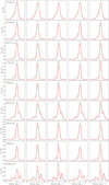 |
Fig. 1 Cloud-averaged spectra of five example toy clouds. Each column corresponds to a cloud and each row to an emission line. The solid red line displays the average spectra of the toy clouds, and the dotted gray line shows the average spectra of ORION-B. The column density and velocity fields corresponding to these toy clouds are shown in Figure 2. |
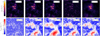 |
Fig. 2 Top: fBm column density maps corresponding to the toy clouds of Figure 1. Bottom: fBm velocity field maps of the toy clouds. |
4.2 Distribution of toy cloud linewidths
Figure 3 presents the distributions of the cloud linewidths, as measured from the mean spectrum of each toy cloud for each of the studied emission lines. The distributions are represented using a box-and-whisker plot. For each emission line, the box indicates the interquartile range, and the whiskers extend to 1% and 99%. The median value of the mean spectrum linewidth for the 1000 toy clouds is indicated with a solid orange line, and the value measured from the true ORION-B cube is indicated with a dashed red line. As explained in Section 3.2, we use the second moment as our linewidth estimator. This can lead to artificially large linewidths for HCN (J=1→0) and N2H+ (J=1→0) due to their hyperfine structure (HFS). Therefore we measured the second moment on the main component of the HCN (J=1→0) and N2H+ (J = 1 → 0) spectra.
The median of the cloud 12CO (J=1→0) linewidths is 2.17 km s−1. This is significantly higher than for the other emission lines. The median of the cloud linewidths for the 13CO (J=1→0), HCO+ (J=1→0) and HCN (J=1→0) lines are similar, ranging from 1.45 km s−1 to 1.54 km s−1. HNC (J=1→0) and 12CS (J = 2 1) display linewidths of respectively 1.37 and 1.26 km s−1. Finally C18O (J=1→0), 32SO (NJ = 32 21), and N2H+ (J=1→0) lines have the lowest median linewidth, ranging from 1.16 to 1.20 km s−1. 12CO (J=1→0) is thus the only emission line whose width clearly exceeds the velocity field amplitude (1.45 km s−1) imposed on the toy clouds. The width of the cloud linewidth distribution also varies among the studied emission lines. The 12CO (J=1→0) line exhibits the smallest range of linewidths, namely, 0.05 km s−1 (2% of the median linewidth). The linewidth distributions for the 13CO (J=1→0), HCO+ (J=1→0) and HNC (J=1→0) lines have larger standard deviations, between 0.075 km s−1 (5%) and 0.11 km s−1 (8%). The distributions of the other emission lines have the largest standard deviations, ranging from 0.122 km s−1 (10%) for 12CS (J = 2 1) to 0.162 km s−1 (14%) for N2H+ (J=1→0).
Unlike the other emission lines, the Orion B cloud-averaged C18O (J=1→0) and N2H+ (J = 1 → 0) linewidth respectively sit below and above the median value obtained from the toy clouds, although still within a standard deviation. For C18O (J=1→0), we suspect that the offset of the C18O (J=1→0) value is due to secondary velocity components present in the Orion B spectra (Gaudel et al. 2023). When generating the clouds, the spectra are shifted along the velocity axis to match the generated velocity field. This shift is done using the location of the brightest velocity component in each spectra as velocity reference. As a result, after averaging, the secondary velocity components end up in the shoulder of the cloud-averaged spectrum. This tends to slightly broaden the average spectra. This is especially visible for C18O (J=1→0), as the Orion B cloud-averaged linewidth of C18O (J=1→0) is the smallest amongst of all the lines considered here, both on a pixel and cloud scale. Moreover, it is the emission line for which the secondary components are the brightest relative to the main velocity component. The offset of the N2H+ (J=1→0) is more puzzling. The line being very faint, this might be due to noise left in the masked data. We suspect that coherent, additive noise might be slightly increasing the Orion B average N2H+ (J=1→0) linewidth. After projecting the spectra on a new velocity field for the toy clouds, this coherence is lost, reducing the wings of the N2H+ (J=1→0) spectra and consequently their linewidth.
It should also be noted that the βvel parameter only has a very limited impact on the beam-average linewidth distributions, as shown in Appendix D. Restricting the range of βvel to what is expected for standard, developed turbulence (βvel∈[2.7, 3]) does not change the statistics derived above.
Figure 4 presents the correlation between the linewidths measured for the toy clouds for three different pairs of emission lines. We do not show all possible combinations for clarity; the pairs in Figure 4 are chosen to illustrate the different trends observed for the whole dataset. For lines that have a similar average linewidth, the individual measurements show a strong degree of correlation. This is the case, for instance, for C18O (J=1→0) and 12CS (J = 2 1), and for 32SO (NJ = 3221)and N2H+ (J=1→0)(the latter is not shown Figure 4). A much weaker correlation is observed for emission lines with different average line widths, for instance 13CO (J=1→0) and N2H+ (J=1→0).
While the velocity field structure (parametrised by βvel) varies among our toy cloud models, the amplitude of the velocity field remains fixed at |v| = 1.45 km s−1. The mixture of intrinsic (i.e., per-pixel) linewidths is by construction the same for all toy clouds since the spectra are sampled from the ORION-B data. The variation in the mean spectrum linewidths for a single emission line therefore only reflects the distribution of the emission in ppv space, notably that of the centroid velocity, rather than differences in the amplitude of the velocity field or changes in the pixel-scale line profiles shapes.
In summary, the mean spectra of the bright and spatially extended 12CO (J=1→0) emission tend to display broad average linewidths that are comparable to the velocity field amplitude that we impose for all our toy clouds. This is expected since the emission of 12CO (J=1→0) is present throughout almost all of the cube (which we treat here as the cloud’s boundary). This supports the long-standing practice to interpret the cloud-averaged linewidth of low-J CO isotopologues as a measure of the overall turbulent motions of the CO-emitting gas within the cloud volume, even though the measurement is a combination of the velocity field’s large-scale gradient and the intrinsic linewidth of each spectrum within the cloud. Under conditions typical of Galactic clouds, the intrinsic linewdith of 12CO (J=1→0) is moreover affected by opacity broadening (see e.g., Correia et al. 2014; Hacar et al. 2016, for a detailed discussion of this effect).
The emission lines fainter than 12CO (J=1→0) exhibit narrower cloud linewidths overall, and there are larger variations among the different toy clouds. This variability of the cloud-averaged linewidth for the fainter lines can be explained by the covering fraction of the emission. Lines such as C18O (J=1→0), 32SO (NJ = 32 21) and N2H+ (J=1→0) are typically detected along sightlines with higher densities than 12CO (J=1→0) or 13CO (J=1→0), and tend to be concentrated in clumps and filamentary structures. On one hand, if these high density regions are uniformly distributed throughout the cloud, then their centroid velocities will span the full range of values in the cloud’s velocity field. On the other hand, when the regions of high density are clustered together, the sampled range of velocities is restricted and the cloud-averaged linewidth for these lines is narrower.
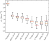 |
Fig. 3 Distribution of the cloud-averaged linewidth of the 1000 randomly generated toy clouds (see Sect. 3.1.2). Each boxplot corresponds to an emission line. The red dashed lines correspond to the Orion B cloud-averaged value. |
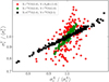 |
Fig. 4 Correlation between different emission lines’ cloud-averaged linewidth. The linewidths have been normalised by their average value over the 1000 randomly generated toy clouds. Each colour corresponds to a correlation between a specific pair of emission lines. |
 |
Fig. 5 Distribution of the cloud-averaged peak temperature of the 1000 randomly generated toy models (see Sect. 3.1.2). Each boxplot corresponds to an emission line, in a smiliar fashion to Figure 3. The distributions are normalised by their average value. The red dashed lines correspond to the Orion B cloud-averaged values also normalised by the toy clouds’ average values. |
4.3 Distribution of the cloud peak brightness temperature
Figure 5 shows the distributions of the peak temperature of the mean spectra for each emission line of all 1000 toy clouds. Since the intrinsic intensity of the emission lines ranges several orders of magnitude, the distributions have been normalised by their mean value to better visualise the width of the distributions.
Absolute values for the mean value and the width of the distributions in Figure 5 are reported in Table 2, as well as values for the peak temperature distributions measured from pixel-scale spectra.
The 12CO (J=1→0) line shows the highest cloud-averaged peak brightness temperature, with a mean of 5.6 K (34% lower than the average pixel-scale 12CO (J=1→0) peak temperature). The average 13CO (J=1→0) peak temperature is ~1 K (46% lower than the average pixel scale peak temperature). The average peak temperatures of the mean spectra for the remaining emission lines are much fainter, and they also tend to show a larger difference relative to the pixel-scale average. The width of the peak temperature distributions also varies systematically: lines with higher cloud-averaged peak temperatures tend to show the least variation across the toy cloud sample. The dispersion in the 12CO (J=1→0) peak temperatures is only 3%, increasing to ~ 24% for the faintest line, N2H+ (J=1→0).
Similarly to the Orion B average N2H+ (J=1→0) and C18O (J=1→0) linewidth values in Figure 3, the Orion B average HNC (J=1→0) peak brightness temperature is offset from the toy clouds median value, although the measurement is still within the 16–84% percentile interval of the toy cloud distribution. A probable cause of this offset is the low level, spatially correlated noise structures in the original HNC (J=1→0) ORION B data that do not average out and lead to a negative bias in the measurement. However, this noise becomes decorrelated in the toy clouds, owing to the spatial and spectral redistribution of the observed spectra.
As for the linewidth of the mean spectra, emission lines with comparable peak temperatures across the cloud sample show a strong linear correlation of their cloud scale peak temperature. This is seen in Figure 6, which presents the correlation between the cloud-averaged peak brightness temperature for three different pairs of emission lines. Again, we show the correlation for only a subset of pairs that illustrate the trends observed across the full suite of lines. The cloud-averaged peak temperature of 12CS (J = 2 1) and C18O (J=1→0) are very tightly correlated, while the peak brightness temperatures of 13CO (J=1→0) and N2H+ (J=1→0) are only weakly correlated.
Since our spectra are sampled from the ORION-B dataset, the total flux of the toy clouds is fixed by construction. The variation in the mean spectrum peak temperature of the toy clouds plotted in Figure 5 is thus linked to the variation in the linewidth of the mean spectrum: higher cloud peak temperatures are associated with emission configurations where the emission is more concentrated in p-p-v space, and therefore with narrower mean linewidths.
Mean and standard deviation of both the cloud-averaged peak brightness temperature and linewidth distributions across the 1000 toy clouds and Orion B.
 |
Fig. 6 Correlation between different emission lines’ cloud-averaged peak brightness temperature. The peak brightness temperature measurements have been normalised by their average value over the 1000 randomly generated toy clouds. Each colour corresponds to a correlation between a specific pair of emission lines. |
4.4 Variation of the line profile shape
In addition to the peak brightness and linewidth of the mean spectra of our toy clouds, we investigated whether the column density and velocity fields have an impact on the typical shape of the spectra. We quantify line profile shape variations and complexity by fitting a Gaussian to each cloud-averaged spectra, and then computing normalised residuals as the sum of the squared residuals for each spectrum divided by the spectrum integrated intensity. The two panels in Figure 7 show the normalised residuals as a function of the velocity field (left panel) and column density field spectral index (right panel) for all the sampled column density fBm indices. We divided the cloud sample into eight equally sized bins of fBm velocity field spectral index. The mean and standard deviation of the bins are displayed using a dashed line and shaded region, respectively.
Overall, the brighter, more spatially extended emission lines exhibit lower normalised residuals than the fainter lines, indicating that they are better represented by a single Gaussian line profile. The value of fBm column density index does not appear to affect the shape of the cloud spectra for our adopted range of βW ∈ [2, 4]. By contrast, the deviation of the cloud spectrum from a Gaussian shape increases with the input fBm velocity index. For βvel = 2, the typical deviation is ~ 20% for all emission lines, while for βvel = 4 the typical deviation ranges from 25% for 12CO (J=1→0) to almost 50% for 32SO (NJ = 32 21). Significant differences between the trends of the various emission lines start to appear at βvel ≥ 3, outside the range of βvel predicted by standard ISM turbulence models, such as Kolmogorov’s or Burger’s turbulence (2.7 < βvel < 3).
 |
Fig. 7 Left: residuals of a Gaussian fit of the beam-average line profiles, as a function of the sub-beam column density field βW index. The sample of 1000 toy clouds is divided in eight equally sized bins of column density field βW index. The full lines and filled range show the mean and standard deviation of the bins. Each colour represents a different emission line. Right: residuals of a Gaussian fit of the beam-average line profiles, as a function of the sub-beam velocity field βv index, in a similar fashion to the left plot. |
5 Discussion
Our aim in this paper has been to quantify the effect of limited spatial resolution on emission line profile parameters using real observational data. More specifically, we have investigated the variability in line profile shapes that can be attributed solely to the sub-beam emission distribution, using mock cloud observations generated from high-resolution observations of the Orion B molecular cloud.
For the analysis in Section 4, we used the term cloud-averaged spectrum to indicate the mean spectrum constructed by averaging the line profiles across our toy clouds. This is because we chose the boundaries of our averaging region to correspond to the size of our box (~20 × 20 pc, which is comparable to the beam size of recent extragalactic wide-field mapping surveys with ALMA) For the rest of this discussion, where we consider the implication of our results more generally, we use the term beam-averaged.
Section 4 showed that the linewidth of the beam-averaged line profiles of 12CO (J=1→0) are significantly larger than the other emission lines in the ORION-B dataset. The beam-averaged 12CO (J=1→0) linewidth is also only weakly affected by the sub-beam distribution of the emission, with variations of less than 10% across all 1000 toy clouds. Likewise, the 12CO (J=1→0) linewidth shows the best correspondence with the sub-beam amplitude of the velocity field. These findings, while not unexpected, support the widespread usage of the 12CO (J=1→0) linewidth on the molecular cloud scale in the extragalactic community as a reliable tracer of cloud’s turbulent motions.
On the other hand, the beam-averaged linewidth of fainter lines, such as the CO isotopologues or high dipole moment tracers, are systematically narrower than the 12CO (J=1→0) linewidth. The linewidth of the cloud-averaged spectrum of the fainter emission lines is also more contingent upon their emission’s sub-beam distribution, with variations of up to a factor 2 for N2H+ (J=1→0). This variability in the beam-averaged linewidths is intrinsic, that is, it is present regardless of the method that is used to estimate the linewidth (e.g. , moment-based calculation, Gaussian profile fitting). It is a source of uncertainty that propagates to several common metrics for the physical properties of clouds that are estimated from the linewidth of molecular emission, such as the virial parameter, density, and free-fall time.
The cloud-averaged peak brightness temperature shows similar trends. The variations of the 12CO (J=1→0) beam-averaged peak brightness temperature do not exceed 10% among our toy clouds. The cloud-averaged peak brightness temperature of fainter emission lines exhibits much larger variation, and is greatest for N2H+ (J = 1 0) among the lines that we consider.
We can understand these general results as follows. The dependence of the line profile parameters on the configuration of the emission in ppv space at scales below the telescope’s resolution is related to the covering fraction of the emission, and how the emitting regions of density dependent tracers sample the underlying velocity field in the gas. The beam-averaged line profile is representative of the sub-beam velocity field in the line-emitting gas. If there is no correlation between the velocity and density fields, then the emission of any line would be distributed randomly throughout the velocity field. For a readily excited emission line like 12CO (J=1→0), the emission emerges throughout the cloud volume and fully explores the velocity field, such that the beam averaged line profile is relatively insensitive to the precise configuration of the emission in ppv space. Conversely, a smaller covering fraction results in larger variability among the beam-averaged line profiles. For instance, the beam-averaged line profile for an emission line that is only excited at high densities depends on the relative motions of the discrete elements of dense gas, and how they are distributed within the bulk of the more diffuse gas within the cloud. Figure 8 illustrates the tight relation between the variability of the beam-averaged linewidth and peak brightness temperature and the covering fraction of the emission for our toy cloud sample.
A trend of decreasing linewidth with increasing gas density traced is observed in both numerical simulations (e.g., Yuan et al. 2020) and Galactic observations (e.g., Heyer et al. 1996; Hacar et al. 2016). It is often considered to be evidence of the size-linewidth relation that characterises the turbulent motions in the molecular ISM, that is higher density regions occupy a more limited volume of the cloud and thus a more limited range of velocities; they are enveloped in regions of lower densities with a larger range of velocities. Extragalactic observations do not always show this behaviour clearly, however, especially in faint or low metallicity environments (Anderson et al. 2014; Nayana et al. 2020).
We emphasise that the variability of the unresolved line parameters reported in this study is not a complete description of the variations that should be present in actual extragalactic measurements for several reasons. First, the covering fraction of an emission line across a cloud is not universal and our results are constrained (by construction) to the characteristics of the emission in the ORION-B dataset. An emission line’s spatial extent is set by the spatial distribution of the H2 column density, which itself is determined by the volume density distribution. The gas temperature, local radiation field intensity and chemical reactions will alter excitation conditions and molecular abundances across the cloud, further affecting the covering fraction of the emission. It is likely, for example, that more diffuse or lower metallicity molecular clouds would exhibit a lower covering fractions of their 12CO (J=1→0) emission, and thus more variation in their cloud-averaged 12CO (J=1→0) line parameters. Second, the velocity fields of real molecular clouds may be considerably more complex than the fBm case that we have used to generate our toy clouds. For a region with different emission components moving at different relative speeds, the beam-averaged spectrum is the sum of each component’s spectrum. If the velocity offset between the components is larger than twice their intrinsic velocity dispersion, the beam-averaged spectrum width becomes representative of the maximum velocity offset between the different components. For example, in a hypothetical cloud where regions of dense gas are moving at a relatively high velocity relative to the systemic velocity of the cloud, then the linewidths of the emission lines excited at high densities could match the linewidths of gas excited at lower densities. This blending of different velocity components becomes more likely as the region size included in the averaging increases, since more structures with larger velocity offsets are averaged together (see Hacar et al. 2016, for a more complete discussion of these blending effects).
A number of other uncertainty sources have not been investigated in this analysis, such as the noise level, spectral resolution and opacity broadening. These issues have been addressed in other works by, for example, Yuan et al. (2020) who studied biases in line width measurements of different emission lines finding that finite spectral resolution and limited sensitivity suppresses line profile wings and producing a bias towards smaller measured velocity dispersions. Hacar et al. (2016), on the other hand, demonstrated that opacity broadening effects significantly alter the line profiles of 12CO (J=1→0), increasing the measured linewidth by a factor 2 to 3. While optical depth effects likely broaden the estimated line widths of 12CO (J=1→0) emission along individual sightlines in Orion B, we do not expect opacity broadening to be the driving factor behind the beam average 12CO (J=1→0) linewidths that we study here for two principal reasons. First, the overall velocity field amplitude is larger than the expected 12CO (J=1→0) linewidth broadening of the pixel scale spectra. More specifically, the velocity field of our toy clouds spans more than 6 km s−1, while the typical pixel scale 12CO (J=1→0) linewidth is 2.2 km s−1 of 2.2 km s−1 (Table 1). This value is itself driven by the velocity separation between the main and the secondary velocity components in Orion B, which have a velocity offset of 4 km s−1 (Gaudel et al. 2023): the average 12CO (J=1→0) linewidth of the main velocity component, responsible for 80% of the total 12CO (J=1→0)emission in Orion B, is only 1.1 km s−1. Second, since the molecular gas column density distribution in Oriong B is overall log-normal, most of the 12CO (J=1→0) spectra arise from lower to moderate density gas where opacity broadening is limited. Specifically, 76% of the total 12CO (J=1→0) intensity stems from very low (AV 1–2) and low (AV 2–6) visual extinction sightlines, as defined in Pety et al. (2017), with only 3% of the total emission arising from high visual extinction sightlines (AV 15–222). Figure 3 shows that a single value of the adopted velocity field amplitude yields cloud-averaged linewidth distributions that are a good match to both optically thin and optically thick emission line tracers in the ORION-B dataset. This tends to support our interpretation of a minor role for opacity broadening in the cloud-averaged 12CO (J=1→0) linewidths.
Leroy et al. (2017) have discussed the possibility of retrieving information about the sub-beam molecular gas density distributions using combinations of line integrated intensities, leveraging the density-dependent excitation of different emission lines. Our analysis suggests that using combinations of emission lines might also yield information about the sub-beam velocity field, by using line spectra instead of integrated intensities. In Section 4.4, we found that the beam average line profiles of dense gas tracers 32SO (NJ = 32 21), N2H+ (J=1→0), 12CS (J = 2 1) and C18O (J=1→0) become increasingly non-Gaussian as the velocity field fBm index increased, while the line profiles of bulk gas tracers 12CO (J=1→0), 13CO (J=1→0) and HCO+ (J=1→0) remained largely Gaussian. This suggests that information about the power law index of the turbulent component of the sub-beam velocity field is encoded in dense gas line profiles and potentially accessible, although we note that the departures become more evident for βvel values outside the range that characterises Kolmogorov (βvel = 2.67) and Burgers (βvel = 3) turbulence.
Our assumption of decorrelated density and velocity fields is also an important simplification, since compressible turbulence in molecular clouds can, through shocks, set regions of higher density where gravitational collapse can be triggered (e.g., Klessen et al. 2000). However, this assumption is relevant as a first order approximation for this study, since it gives a qualitative understanding and a lower limit of the potential variability of line profile due to sub-beam distribution of the gas. More quantitatively, Brunt & Federrath (2014) presented a method to retrieve the relative fractions of solenoidal and compressible modes in interstellar clouds. This method requires an estimation of the correlation between density and velocity fields through the parameter ϵ, with ϵ = 0 corresponding to uncorrelated density and velocity fields. They directly measure ϵ from numerical simulations and also estimate it using line observations from core to ~100 p˙c scales. They report ϵ values of 0.1 on average, with an upper limit of 0.15 in the specific case of Orion B (Orkisz et al. 2017), which suggest weakly correlated density and velocity fields. Moreover, we check our assumption of decorrelated fields by manually introducing a level of correlation in the fBm structures, similarly to Miville-Deschênes et al. (2003). We find that introducing a weak to moderate correlation between the column density and velocity fields does not change our results (see Appendix B).
Recent literature includes several examples of methods to generate scalar and vector fields that are more representative of the turbulent ISM than the simple fBm structures that we have used in this paper. For example, Régaldo-Saint Blancard et al. (2023) have presented an algorithm that is able to generate column density fields from simulated or observational data using wavelet phase harmonic statistics of the input image. Without GPU acceleration, however, the method is too computationally expensive to assemble a large (N > 100) repository of toy clouds. Durrive et al. (2022) have devised an analytic generator of three-dimensional incompressible magnetohydrodynamic turbulence that uses a deterministic transform applied to a random Gaussian field, resulting in a multifractal random field. This method has the advantage of relying on few parameters with clear geometric interpretation, and it is computationally fast. A possible avenue for extending this work would be to use these (or similar) methods to generate more physically realistic turbulent molecular cloud models, which could be then associated to molecular line emission via pairing with suitable observational data (the approach adopted in this paper) or statistical equilibrium calculations of spectral line luminosities, for example with public codes like RADEX (van der Tak et al. 2007) or DESPOTIC (Krumholz 2014).
Highly resolved multiline surveys of Milky-Way clouds, such as the ORION B program (Pety et al. 2017), the LEGO survey (Barnes et al. 2020) or stratified random sampling observations (Tafalla et al. 2021, 2023) opens several avenues for helping our understanding of spatially unresolved measurements of molecular line emission. One straightforward approach would be to directly compare spatially unresolved spectra and their parameters to the average Orion B spectrum. This would allow to detect Orion B like clouds, or conversely detect departures of the gas properties from the typical conditions found in Orion B.
Another promising line of inquiry enabled by the rich, highly spatial resolution, wide bandwidth surveys of Galactic molecular clouds like ORION B is a detailed empirical understanding of excitation mechanisms within molecular clouds down to the spatial scale of cold cores. A notable study in that direction was conducted by Santa-Maria et al. (2023), who studied HCN (J=1→0) emission in the Orion B cloud as a function of NH2 and G0. They highlighted how a substantial fraction of the HCN (J=1→0) emission in Orion B arise from low density, illuminated gas. Overall, understanding the relationship between line intensities and molecular gas properties, such as density, temperature, and radiation field, is crucial for accurately estimating gas properties from unresolved observations. Indeed, the observed integrated intensity averaged over a beam equals the sum of the sub-beam gas properties distribution multiplied by the integrated intensity as a function of those properties. In that regard, the integrated intensity is a key line profile parameter. This observable has not been studied here as it will be the subject of a future paper aimed at deriving the sub-beam density distribution using the integrated intensity line ratios of unresolved observations (Zakardjian et al, in prep).
 |
Fig. 8 Left: maximum variation (1–99% percentile range divided by the mean) of the cloud-averaged linewidth distribution of the toy cloud sample, as a function of emission line covering fraction. Right: maximum variation of the beam average peak brightness temperature distribution of the toy cloud sample, as a function of emission line covering fraction. |
6 Summary and conclusions
This paper is part of a series that uses the ORION-B survey data as a template for interpreting unresolved extra galactic observations of molecular gas. Here, we focused on the variation in unresolved line properties that can be attributed to spatial averaging within the resolution element of a telescope. Unresolved observations are a spatial average of emission that is structured on much smaller scales in p-p-v space. The mean spectrum resulting from this spatial averaging thus depends on the sub-beam distribution of the emission. Consequently, beam-averaging can introduce a non-negligible uncertainty to ‘global’ measurements of molecular cloud properties, since the line parameters of unresolved spectra can vary, even though the underlying distribution of molecular gas properties are similar.
We generated toy molecular cloud intensity and velocity fields using the fBm approach presented by Stutzki et al. (1998), varying the Fourier power spectra index between 2 and 4 for both βW and βvel. We combined these fields with spectra sampled from the high-resolution multiline ORION-B survey to build a sample of 1000 toy molecular clouds, each with corresponding datacube for the common molecular emission lines 12CO (J=1→0), 13CO (J=1→0), C18O (J=1→0), HCO+ (J=1→0), HCN (J=1→0), HNC (J=1→0), 12CS (J = 2 1), 32SO (NJ = 32 21) and N2H+ (J=1→0). By construction, the total flux, the size and the velocity field amplitude of the toy clouds are fixed. The distributions of the emission line peak brightness, linewidth and integrated intensity at the pixel scale of the toy clouds are also identical. Ratios between the line properties of different emission lines at the pixel scale are likewise fixed. The sole difference between the toy clouds is the organisation of the emission in p-p-v. space, which is determined by the intensity and velocity fields that we use to generate the toy clouds.
With our sample of toy clouds, we investigated how much variation in the cloud-averaged line profiles can arise due to beam-smearing of the spatial and spectral organisation of the emission within the clouds, and whether there is information about the cloud’s underlying velocity and intensity structure that can be recovered from the cloud-averaged line profiles. Our main results are the following:
The beam-averaged line properties (peak temperature, linewidth and line profile shape) of 12CO (J=1→0) show the smallest variation with the morphology of the sub-beam column density and velocity fields (as parameterised by βW and βvel respectively) among all the emission lines that we studied. Across our full sample of toy clouds, the fluctuation (σX/<X>) in all the beam-averaged 12CO (J=1→0) line properties is 2.2% and the maximum variation (1–99% percentile range divided by the mean) is 12%;
The beam-averaged line properties of the other emission lines show noticeably more variation. 13CO (J=1→0), HCO+ (J=1→0) and HNC (J=1→0) display line properties fluctuations of 5 to 8% and maximum variations between 26 and 43%; 12CS (J = 2 1), C18O (J=1→0), HCN (J=1→0) and 32SO (NJ = 32 21) show line properties variations of ~11%, and maximum variations ranging from 50 to 60%. N2H+ (J=1→0) displays the largest variations of its line properties due to beam dilution, with maximum variations reaching a factor 2;
The magnitude of the fluctuations in the properties determined from an unresolved emission line is linearly correlated with the covering fraction of the emission line;
The beam-averaged linewidths of 12CO (J=1→0) best reflect the amplitude of the sub-beam velocity field that we impose. The 12CO (J=1→0) linewidth reaches on average 50% of the full velocity field range and matches the 16–84% percentile range of the velocity field, with a relative standard deviation of 2.2%;
Unresolved line profiles of C18O (J=1→0), 12CS (J = 2→1), HNC (J=1→0) and 32SO (NJ = 32→21) deviate significantly from a Gaussian shape as the sub-beam velocity field spectral index βvel increases. These deviations become significant when βvel > 3, outside the range of βvel associated with typical ISM turbulence models. By contrast, the unresolved line profiles of 12CO (J=1→0), 13CO (J=1→0) and HCO+ (J = 1→0) are only weakly affected by the velocity field spectral index.
Our results suggest several avenues for future investigation. These include generating and studying clouds of different mass, star-forming activity and situated in different environments (e.g., quiescent clouds without massive star formation, or clouds in the Central Molecular Zone). Two axes of the parameter space could also be explored more systematically, namely the beam size (averaging scale) and the velocity field amplitude. Another avenue to explore would be to add complexity to the velocity fields by including large scale motions, such as cloud scale velocity gradients and galactic scale motions, or by adding smaller scale motions, for instance gravitational collapse. In that regard, incorporating a degree of correlation between the density and velocity fields would be essential.
An alternative outlook on the interpretation of spatially unresolved measurements of molecular line emission is estimating the sub-beam statistical distribution of gas properties, notably the molecular gas density. Estimating this sub-beam gas density distribution is a crucial problem, as the gas density plays a critical role in setting the star formation rate per unit gas. This problem is commonly solved using integrated intensity ratios of the different emission lines considered in this work (Schinnerer & Leroy 2024, Section 3). The integrated intensity, therefore an essential emission line property, will be the subject of a forthcoming paper focused on determining the sub-beam gas density distribution through the integrated intensity of multiple emission lines (Zakardjian et al., in prep).
Acknowledgements
This work was supported in part by the French Agence Nationale de la Recherche through the DAOISM grant ANR-21-CE31-0010 and by the Programme National “Physique et Chimie du Milieu Interstellaire” (PCMI) of CNRS/INSU with INC/INP, co-funded by CEA and CNES. Part of this research was carried out at the Jet Propulsion Laboratory, California Institute of Technology, under a contract with the National Aeronautics and Space Administration (80NM0018D0004). This research has made use of data from the Herschel Gould Belt Survey (HGBS) project (http://gouldbelt-herschel.cea.fr). The HGBS is a Herschel Key Programme jointly carried out by SPIRE Specialist Astronomy Group 3 (SAG 3), scientists of several institutes in the PACS Consortium (CEA Saclay, INAF-IFSI Rome and INAF-Arcetri, KU Leuven, MPIA Heidelberg), and scientists of the Herschel Science Center (HSC). MGSM acknowledges support from the NSF under grant CAREER 2142300. JRG and MGSM thank the Spanish MICINN for funding support under grant PID2019-106110GB-I00.
References
- Anderson, C. N., Meier, D. S., Ott, J., et al. 2014, ApJ, 793, 37 [CrossRef] [Google Scholar]
- André, P., Men’shchikov, A., Bontemps, S., et al. 2010, A&A, 518, L102 [NASA ADS] [CrossRef] [EDP Sciences] [Google Scholar]
- Arzoumanian, D., André, P., Didelon, P., et al. 2011, A&A, 529, L6 [NASA ADS] [CrossRef] [EDP Sciences] [Google Scholar]
- Baker, P. L. 1976, A&A, 50, 327 [NASA ADS] [Google Scholar]
- Barnes, A. T., Kauffmann, J., Bigiel, F., et al. 2020, MNRAS, 497, 1972 [NASA ADS] [CrossRef] [Google Scholar]
- Bensch, F., Stutzki, J., & Ossenkopf, V. 2001, A&A, 366, 636 [NASA ADS] [CrossRef] [EDP Sciences] [Google Scholar]
- Boldyrev, S. 2002, ApJ, 569, 841 [NASA ADS] [CrossRef] [Google Scholar]
- Brunt, C. M., & Federrath, C. 2014, MNRAS, 442, 1451 [Google Scholar]
- Brunt, C. M., & Heyer, M. H. 2002, ApJ, 566, 276 [Google Scholar]
- Cao, Z., Jiang, B., Zhao, H., & Sun, M. 2023, ApJ, 945, 132 [NASA ADS] [CrossRef] [Google Scholar]
- Correia, C., Burkhart, B., Lazarian, A., et al. 2014, ApJ, 785, L1 [Google Scholar]
- Dib, Sami, Bontemps, Sylvain, Schneider, Nicola, et al. 2020, A&A, 642, A177 [NASA ADS] [CrossRef] [EDP Sciences] [Google Scholar]
- Dickman, R., Snell, R. L., & Schloerb, F. P. 1986, ApJ, 309, 326 [NASA ADS] [CrossRef] [Google Scholar]
- Durrive, J.-B., Changmai, M., Keppens, R., et al. 2022, Phys. Rev. E, 106, 025307 [Google Scholar]
- Einig, L., Pety, J., Roueff, A., et al. 2023, A&A, 677, A158 [NASA ADS] [CrossRef] [EDP Sciences] [Google Scholar]
- Elmegreen, B. G., & Scalo, J. 2004, Annu. Rev. Astron. Astrophys., 42, 211 [Google Scholar]
- Gaudel, M., Orkisz, J. H., Gerin, M., et al. 2023, A&A, 670, A59 [NASA ADS] [CrossRef] [EDP Sciences] [Google Scholar]
- Hacar, A., Alves, J., Burkert, A., & Goldsmith, P. 2016, A&A, 591, A104 [NASA ADS] [CrossRef] [EDP Sciences] [Google Scholar]
- Hennebelle, P., & Falgarone, E. 2012, A&A Rev., 20, 55 [NASA ADS] [CrossRef] [Google Scholar]
- Heyer, M., & Dame, T. M. 2015, ARA&A, 53, 583 [Google Scholar]
- Heyer, M. H., Carpenter, J. M., & Ladd, E. F. 1996, ApJ, 463, 630 [Google Scholar]
- Klessen, R. S., Heitsch, F., & Mac Low, M.-M. 2000, ApJ, 535, 887 [NASA ADS] [CrossRef] [Google Scholar]
- Krumholz, M. R. 2014, MNRAS, 437, 1662 [NASA ADS] [CrossRef] [Google Scholar]
- Leroy, A. K., Usero, A., Schruba, A., et al. 2017, ApJ, 835, 217 [NASA ADS] [CrossRef] [Google Scholar]
- Leroy, A. K., Schinnerer, E., Hughes, A., et al. 2021, ApJS, 257, 43 [NASA ADS] [CrossRef] [Google Scholar]
- Leung, C. M. 1978, ApJ, 225, 427 [NASA ADS] [CrossRef] [Google Scholar]
- Levrier, F., Neveu, J., Falgarone, E., et al. 2018, A&A, 614, A124 [NASA ADS] [CrossRef] [EDP Sciences] [Google Scholar]
- Lombardi, M., Bouy, H., Alves, J., & Lada, C. J. 2014, A&A, 566, A45 [NASA ADS] [CrossRef] [EDP Sciences] [Google Scholar]
- Miville-Deschênes, M. A., Levrier, F., & Falgarone, E. 2003, ApJ, 593, 831 [Google Scholar]
- Nayana, A. J., Naslim, N., Onishi, T., et al. 2020, ApJ, 902, 140 [Google Scholar]
- Orkisz, J. H., Pety, J., Gerin, M., et al. 2017, A&A, 599, A99 [NASA ADS] [CrossRef] [EDP Sciences] [Google Scholar]
- Pety, J., Guzmán, V. V., Orkisz, J. H., et al. 2017, A&A, 599, A98 [NASA ADS] [CrossRef] [EDP Sciences] [Google Scholar]
- Planck Collaboration I. 2014, A&A, 571, A1 [NASA ADS] [CrossRef] [EDP Sciences] [Google Scholar]
- Régaldo-Saint Blancard, B., Allys, E., Auclair, C., et al. 2023, ApJ, 943, 9 [CrossRef] [Google Scholar]
- Russeil, D., Schneider, N., Anderson, L. D., et al. 2013, A&A, 554, A42 [NASA ADS] [CrossRef] [EDP Sciences] [Google Scholar]
- Santa-Maria, M. G., Goicoechea, J. R., Pety, J., et al. 2023, A&A, 679, A4 [NASA ADS] [CrossRef] [EDP Sciences] [Google Scholar]
- Scalo, J. M. 1987, in Interstellar Processes, 134, eds. D. J. Hollenbach, J. Thronson, & A. Harley, 349 [Google Scholar]
- Schinnerer, E., & Leroy, A. K. 2024, ARA&A, 62, 369 [NASA ADS] [CrossRef] [Google Scholar]
- Schneider, N., Bontemps, S., Simon, R., et al. 2011, A&A, 529, A1 [NASA ADS] [CrossRef] [EDP Sciences] [Google Scholar]
- Schneider, N., André, P., Könyves, V., et al. 2013, ApJ, 766, L17 [NASA ADS] [CrossRef] [Google Scholar]
- Shetty, R., Glover, S. C., Dullemond, C. P., & Klessen, R. S. 2011, MNRAS, 412, 1686 [NASA ADS] [CrossRef] [Google Scholar]
- Solomon, P., Rivolo, A., Barrett, J., & Yahil, A. 1987, ApJ, 319, 730 [NASA ADS] [CrossRef] [Google Scholar]
- Stutzki, J., Bensch, F., Heithausen, A., Ossenkopf, V., & Zielinsky, M. 1998, A&A, 336, 697 [NASA ADS] [Google Scholar]
- Sun, Y., Yang, J., Yan, Q.-Z., et al. 2021, ApJS, 256, 32 [NASA ADS] [CrossRef] [Google Scholar]
- Tafalla, M., Usero, A., & Hacar, A. 2021, A&A, 646, A97 [NASA ADS] [CrossRef] [EDP Sciences] [Google Scholar]
- Tafalla, M., Usero, A., & Hacar, A. 2023, A&A, 679, A112 [NASA ADS] [CrossRef] [EDP Sciences] [Google Scholar]
- Tauber, J. A., Goldsmith, P. F., & Dickman, R. L. 1991, ApJ, 375, 635 [Google Scholar]
- van der Tak, F. F. S., Black, J. H., Schöier, F. L., Jansen, D. J., & van Dishoeck, E. F. 2007, A&A, 468, 627 [NASA ADS] [CrossRef] [EDP Sciences] [Google Scholar]
- Wolfire, M. G., Hollenbach, D., & Tielens, A. 1993, ApJ, 402, 195 [NASA ADS] [CrossRef] [Google Scholar]
- Yang, Y., Jiang, Z.-B., Chen, Z.-W., et al. 2020, Res. Astron. Astrophys., 20, 115 [CrossRef] [Google Scholar]
- Yuan, Y., Krumholz, M. R., & Burkhart, B. 2020, MNRAS, 498, 2440 [Google Scholar]
- Zuckerman, B., & Evans, N. J., I. 1974, ApJ, 192, L149 [NASA ADS] [CrossRef] [Google Scholar]
Appendix A Histogram matching and spatial filtering
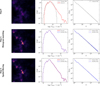 |
Fig. A.1 Top: (From left to right) fBm column density field, statistical distribution of the Orion B (red) and fBm (grey) column densities, and power spectrum of the fBm column density field. For illustrative purposes, the fBm distribution has been scaled to have the same mean and standard deviation as the log column density distribution of Orion B, before being exponentiated. Middle: (From left to right) modified fBm column density field resulting from the histogram matching procedure, statistical distribution of the Orion B (red) and modified fBm (dashed blue) column densities, and power spectrum of the fBm (grey) and modified fBm (dashed blue) column density fields. Bottom: (From left to right) modified fBm column density field resulting from the histogram matching procedure and the spatial filtering process, statistical distribution of the Orion B (red) and modified fBm (dashed blue) column densities, and power spectrum of the fBm (grey) and modified fBm (dashed blue) column density fields. |
Figure A.1 shows a column density fBm field (β = 3), its statistical distribution and power law index before and after applying the histogram matching procedure and spatial filtering process presented in Section 3.1.1. In Figure A.1, the fBm distribution has been exponentiated after being scaled to have the same mean and standard deviation as the log column density distribution of Orion B. This is only for easier comparison with the Orion B column density distribution, and is not necessary in practice to generate mock clouds. The two step process of histogram matching and then spatial filtering makes one cycle that is iteratively repeated until convergence during the toy cloud generation procedure. Convergence is achieved when the toy cloud both matches the Orion B density distribution and the fBm power spectrum, which takes around four repetitions.
Appendix B Column density and velocity field correlation
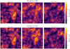 |
Fig. B.1 Left: fBm image of size 512x512 and Fourier spectral index β = 3. Right: Second fBm image of size 512x512 and Fourier spectral index β = 3 with different phases (different seed). Centre: fBm image resulting from introducing 20% (top) and 50%(bottom) of the phase from fBm I into fBm II. |
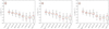 |
Fig. B.2 In a similar fashion to Fig. 3, distributions of the cloud-averaged linewidth of (from left to right) the original cloud set, 20% correlation cloud set and 50% correlation cloud set (see Sect. B). |
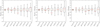 |
Fig. B.3 In a similar fashion to Fig. 5, distributions of the cloud-averaged peak brightness temperature of (from left to right) the original cloud set, 20% correlation cloud set and 50% correlation cloud set (see Sect. B). |
In order to test our assumption of uncorrelated column density and velocity fields, we manually introduced a level correlation between the two by randomly assigning the same phase to a set of points (in Fourier Space) in both fields (similarly to Miville-Deschênes et al. 2003).
Figure B.1 displays two fBm images with different phases (seeds) and the fBm image resulting from setting respectively 20% and 50% of phases in common. Specifically, 20% and 50% of the phases of image II are replaced by phases of image I. Even with a correlation level of 50%, the two fBm images already appear very correlated, with similar large and medium scale structures.
Using this method, we generated two new sets of 200 toy clouds with respectively 20% and 50% of common phases between the column density and velocity fields. Phases of the column density field are “injected” in the velocity field. Figure B.2 shows the resulting cloud-averaged linewidth distributions for both datasets as well as for the original set of toy clouds, in a similar fashion to Figure 3. There is no significant difference between the linewidth distributions of the original dataset and the set of toy clouds with a 20% correlation, except a slightly narrower 1-99% percentile range of the N2H+ (J=1→0) linewidth distribution for the correlated clouds. In the case of the 50% correlation cloud set, a difference with the original dataset is perceptible, but remains marginal. The difference in mean linewidth is still largely under a single standard deviation. This standard deviation of the linewidth distribution is similar for both datasets. The only visible difference is in the 1-99% percentile range, somewhat reduced in the correlated dataset for lines C18O (J=1→0), 32SO (NJ = 32 21) and N2H+ (J=1→0).
Figure B.3 displays the cloud-averaged peak brightness temperature distributions for both correlated toy cloud datasets and the original cloud set, in a similar fashion to Figure 5. Unexpectedly, difference between the correlated and uncorrelated clouds sets are the same as for the linewidth distributions.
Appendix C Using 13CO (J=1→0) velocity at peak as reference
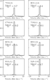 |
Fig. C.1 Histograms of the velocity offset between the 13CO (J=1→0) velocity at peak brightness temperature and the velocity at peak brightness temperatures of other emission lines considered in this work. |
Figure C.1 displays the velocity offset between 13CO (J=1→0) and the other emission lines at pixel scale in the original ORION B datacube. This offset is defined as the difference of velocity at peak brightness temperature. The intensity weighted average velocity offset of each line is also reported on the Figure. This intensity weighted average over the entire datacube is defined as  , with △vi and Ii respectively the velocity offset and integrated intensity at pixel i. In the case of HCO+ (J=1→0), C18O (J=1→0), HCN (J=1→0) and 32SO (NJ = 32 21), the intensity weighted average offset is less than a channel width (0.5k˙m s−1). For the other emission lines, this average offset is equal or less than two channel widths. For all lines the median velocity offset is 0k˙m s−1. As all these velocity offsets are low and consistent with noise related uncertainties, we consider that using the 13CO (J=1→0) velocity at peak brightness temperature for constructing the toy clouds as described in Section 3.1.2 does not introduce any bias in the results.
Appendix D Limited βvel range
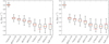 |
Fig. D.1 Distributions of the cloud-averaged linewidth of the original cloud set (left) and the βvel limited cloud set (right, see Sect. D), in a similar fashion to Fig. 3. |
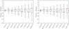 |
Fig. D.2 Distributions of the cloud-averaged peak brightness temperature of the original cloud set (left) and the βvel limited cloud set (right, see Sect. D), in a similar fashion to Fig. 5. |
 |
Fig. D.3 Cloud-average linewidth (left) and peak brightness temperature (right) as a function of the sub-beam velocity field βvel index. The original sample of 1000 toy clouds is divided in six equally sized bins of column density field βW index. The full lines and filled range show the mean and standard deviation of the bins. Each colour represents a different emission line. |
Throughout the paper, the βvel parameter is assumed to vary between 2 and 4. However standard turbulence theory suggests βvel between 2.67 (Kolmogorov turbulence) and 3.0 (Burgers turbulence). Therefore it is worthwhile to check whether the statistics obtained from the extended parameter set βvel ∈ [2, 4] are still representative of the restricted parameter set βvel ∈ [2.67, 3.0]. To confirm this, we have generated a sample of 200 toy clouds with βvel ∈ [2.67, 3.0] and compared the resulting statistics from those of the original dataset. Figure D.1 displays the cloud-averaged linewidth distributions for this new set of clouds as well as for the original set of toy clouds, in a similar fashion to Figure 3. The difference is negligible, with a slightly less extended 1-99% percentile range of the N2H+ (J = 1→0) linewidth distribution in the case of the toy cloud set with limited βvel. Figure D.2 shows the cloud-averaged peak brightness temperature distribution for both datasets as well. The conclusion is the same, the difference between both datasets is marginal. Therefore the statistics retrieved over the full range of βvel is still representative of βvel typical of standard turbulence.
Moreover, the βvel parameter has little impact on the deviations observed in Fig. 4 and 6. Figure D.3 shows how the cloud-averaged linewidths and peak brightness temperatures related to the βvel parameter. Its impact is mostly visible for the fainter lines such as N2H+ (J=1→0), 12CS (J = 2→1), 32SO (NJ = 32→21), HNC (J=1→0) and HCN (J=1→0). But even then, the effect is limited, with a constant average linewidth and slightly increasing standard deviation with increasing βvel. The N2H+ (J = 1→0) linewidth is the exception, with a ~20% variation of the average linewidth across the parameter space. This variation is still within one standard deviation of the entire cloud distribution. Overall, the impact of the βvel parameter on both the cloud-averaged linewidth and peak brightness temperature is limited.
Atacama Large Millimeter/submillimeter Array survey for the Physics at High Angular resolution in Nearby Galaxies project.
For more information about the GILDAS software, see https://www.iram.fr/IRAMFR/GILDAS/
Cloud-scale averaging is alternatively referred to as ‘beam smearing’ by Yuan et al. (2020). We prefer the more generic term ‘cloud-scale averaging’ since ‘beam smearing’ connotes a contribution to the cloud linewidth from the galactic rotation curve in extragalactic literature, which we do not investigate here.
The integrated intensity and cloud mass are fixed by construction.
All Tables
Rest frequencies, critical densities, and typical properties of the subset of emission lines in the ORION-B dataset that we consider in this paper.
Mean and standard deviation of both the cloud-averaged peak brightness temperature and linewidth distributions across the 1000 toy clouds and Orion B.
All Figures
|
Fig. 1 Cloud-averaged spectra of five example toy clouds. Each column corresponds to a cloud and each row to an emission line. The solid red line displays the average spectra of the toy clouds, and the dotted gray line shows the average spectra of ORION-B. The column density and velocity fields corresponding to these toy clouds are shown in Figure 2. |
| In the text | |
|
Fig. 2 Top: fBm column density maps corresponding to the toy clouds of Figure 1. Bottom: fBm velocity field maps of the toy clouds. |
| In the text | |
|
Fig. 3 Distribution of the cloud-averaged linewidth of the 1000 randomly generated toy clouds (see Sect. 3.1.2). Each boxplot corresponds to an emission line. The red dashed lines correspond to the Orion B cloud-averaged value. |
| In the text | |
|
Fig. 4 Correlation between different emission lines’ cloud-averaged linewidth. The linewidths have been normalised by their average value over the 1000 randomly generated toy clouds. Each colour corresponds to a correlation between a specific pair of emission lines. |
| In the text | |
|
Fig. 5 Distribution of the cloud-averaged peak temperature of the 1000 randomly generated toy models (see Sect. 3.1.2). Each boxplot corresponds to an emission line, in a smiliar fashion to Figure 3. The distributions are normalised by their average value. The red dashed lines correspond to the Orion B cloud-averaged values also normalised by the toy clouds’ average values. |
| In the text | |
|
Fig. 6 Correlation between different emission lines’ cloud-averaged peak brightness temperature. The peak brightness temperature measurements have been normalised by their average value over the 1000 randomly generated toy clouds. Each colour corresponds to a correlation between a specific pair of emission lines. |
| In the text | |
|
Fig. 7 Left: residuals of a Gaussian fit of the beam-average line profiles, as a function of the sub-beam column density field βW index. The sample of 1000 toy clouds is divided in eight equally sized bins of column density field βW index. The full lines and filled range show the mean and standard deviation of the bins. Each colour represents a different emission line. Right: residuals of a Gaussian fit of the beam-average line profiles, as a function of the sub-beam velocity field βv index, in a similar fashion to the left plot. |
| In the text | |
|
Fig. 8 Left: maximum variation (1–99% percentile range divided by the mean) of the cloud-averaged linewidth distribution of the toy cloud sample, as a function of emission line covering fraction. Right: maximum variation of the beam average peak brightness temperature distribution of the toy cloud sample, as a function of emission line covering fraction. |
| In the text | |
|
Fig. A.1 Top: (From left to right) fBm column density field, statistical distribution of the Orion B (red) and fBm (grey) column densities, and power spectrum of the fBm column density field. For illustrative purposes, the fBm distribution has been scaled to have the same mean and standard deviation as the log column density distribution of Orion B, before being exponentiated. Middle: (From left to right) modified fBm column density field resulting from the histogram matching procedure, statistical distribution of the Orion B (red) and modified fBm (dashed blue) column densities, and power spectrum of the fBm (grey) and modified fBm (dashed blue) column density fields. Bottom: (From left to right) modified fBm column density field resulting from the histogram matching procedure and the spatial filtering process, statistical distribution of the Orion B (red) and modified fBm (dashed blue) column densities, and power spectrum of the fBm (grey) and modified fBm (dashed blue) column density fields. |
| In the text | |
|
Fig. B.1 Left: fBm image of size 512x512 and Fourier spectral index β = 3. Right: Second fBm image of size 512x512 and Fourier spectral index β = 3 with different phases (different seed). Centre: fBm image resulting from introducing 20% (top) and 50%(bottom) of the phase from fBm I into fBm II. |
| In the text | |
|
Fig. B.2 In a similar fashion to Fig. 3, distributions of the cloud-averaged linewidth of (from left to right) the original cloud set, 20% correlation cloud set and 50% correlation cloud set (see Sect. B). |
| In the text | |
|
Fig. B.3 In a similar fashion to Fig. 5, distributions of the cloud-averaged peak brightness temperature of (from left to right) the original cloud set, 20% correlation cloud set and 50% correlation cloud set (see Sect. B). |
| In the text | |
|
Fig. C.1 Histograms of the velocity offset between the 13CO (J=1→0) velocity at peak brightness temperature and the velocity at peak brightness temperatures of other emission lines considered in this work. |
| In the text | |
|
Fig. D.1 Distributions of the cloud-averaged linewidth of the original cloud set (left) and the βvel limited cloud set (right, see Sect. D), in a similar fashion to Fig. 3. |
| In the text | |
|
Fig. D.2 Distributions of the cloud-averaged peak brightness temperature of the original cloud set (left) and the βvel limited cloud set (right, see Sect. D), in a similar fashion to Fig. 5. |
| In the text | |
|
Fig. D.3 Cloud-average linewidth (left) and peak brightness temperature (right) as a function of the sub-beam velocity field βvel index. The original sample of 1000 toy clouds is divided in six equally sized bins of column density field βW index. The full lines and filled range show the mean and standard deviation of the bins. Each colour represents a different emission line. |
| In the text | |
Current usage metrics show cumulative count of Article Views (full-text article views including HTML views, PDF and ePub downloads, according to the available data) and Abstracts Views on Vision4Press platform.
Data correspond to usage on the plateform after 2015. The current usage metrics is available 48-96 hours after online publication and is updated daily on week days.
Initial download of the metrics may take a while.