| Issue |
A&A
Volume 696, April 2025
|
|
|---|---|---|
| Article Number | A230 | |
| Number of page(s) | 18 | |
| Section | Stellar atmospheres | |
| DOI | https://doi.org/10.1051/0004-6361/202450348 | |
| Published online | 28 April 2025 | |
Characterisation of magnetic activity of M dwarfs
Possible impact on surface brightness
1
Laboratoire Lagrange, Université Côte d’Azur, Observatoire de la Côte d’Azur, CNRS,
Boulevard de l’Observatoire, CS 34229,
06304
Nice Cedex 4,
France
2
Instituto de Astronomía y Física del Espacio (CONICET-UBA),
C.C. 67 Sucursal 28,
C1428EHA
Buenos Aires,
Argentina
3
Departamento de Física, Facultad de Ciencias Exactas y Naturales, Universidad de Buenos Aires,
Buenos Aires,
Argentina
4
Instituto de Ciencias Astronómicas, de la Tierra y del Espacio (ICATE-CONICET),
C.C. 467,
5400
San Juan,
Argentina
5
Facultad de Ciencias Exactas, Físicas y Naturales, Universidad Nacional de San Juan,
San Juan,
Argentina
★ Corresponding author; This email address is being protected from spambots. You need JavaScript enabled to view it.
Received:
12
April
2024
Accepted:
27
February
2025
Abstract
Context. M dwarfs are an ideal laboratory for hunting Earth-like planets, and the study of chromospheric activity is an important part of this task. On the one hand, according to the study of short-term activity their high levels of magnetic activity can affect habitability and make it difficult to detect exoplanets orbiting around them. On the other hand, however, long-term activity studies can show whether or not these stars exhibit cyclical behaviour in their activity, facilitating the detection of planets in periods of low magnetic activity.
Aims. The long-term cyclical behaviour of magnetic activity can be detected by studying several spectral lines and explained by different stellar dynamo models (such as αΩ or α2 dynamos). In the present work, we studied the Mount Wilson S index to search for evidence of long-term activity possibly driven by a solar-type dynamo.
Methods. We studied a sample of 35 M dwarfs with different levels of chromospheric activity and spectral classes ranging from dM0 to dM6. To do this, we used 2965 spectra in the optical range from different instruments installed in the southern and northern hemispheres to construct time series with extensions of up to 21 years. We analysed these time series with different time-domain techniques to detect cyclical patterns. In addition, using 2MASS-KS and visible photometry we also studied the potential impact of chromospheric activity on surface brightness.
Results. Using the colour index (V − KS), we calculated the chromospheric emission levels and found that most of the stars in the sample have low emission levels, indicating that most of them are inactive or very inactive stars. For 31 stars of 35, we constructed time series using the S indexes, and we detected 13 potential cycles of magnetic activity. These cycles have an approximate duration of between three and 19 years, with false alarm probabilities (FAPs) less than 0.1%. For stars that do not show cyclic behaviour, we found that the mean value of the S index varies between 0.350 and 1.765, and its mean variability and chromospheric emission level are around 12% and −5.110 dex, respectively. We do not find any impact of chromospheric activity on the surface brightness in the domain of −5.6 < log R′H K < −4.5.
Key words: techniques: spectroscopic / stars: activity / stars: late-type
Based on data obtained at Complejo Astronómico El Leoncito, operated under the agreement between the Consejo Nacional de Investigaciones Científıcas y Técnicas de la República Argentina and the National Universities of La Plata, Córdoba, and San Juan.
© The Authors 2025
 Open Access article, published by EDP Sciences, under the terms of the Creative Commons Attribution License (https://creativecommons.org/licenses/by/4.0), which permits unrestricted use, distribution, and reproduction in any medium, provided the original work is properly cited.
This article is published in open access under the Subscribe to Open model. This email address is being protected from spambots. You need JavaScript enabled to view it. to support open access publication.
1 Introduction
Stellar magnetic activity is a phenomenon that has been extensively studied using several spectral lines sensitive to chromospheric activity (e.g. Mg II, Ca II, Na I, and Hα) by integrating their fluxes in the line core (Baliunas et al. 1995; Díaz et al. 2007; Lovis et al. 2011; Gomes da Silva et al. 2011, 2012; Buccino et al. 2014; Flores et al. 2016, 2018; Ibañez Bustos et al. 2019a,b, 2020; Di Maio et al. 2020; Lafarga et al. 2021; Mignon et al. 2023). The variability of each flux or equivalent width with time is related to stellar rotation and the evolution of the stellar active regions providing information on different regions at different heights of the stellar atmosphere. The stellar magnetic activity is assumed to be driven by a stellar dynamo that in the case of the Sun is called αΩ dynamo and could be explained by the feedback between the differential rotation (Ω-effect) of the Sun and the α effect related to the turbulent helical movements of the plasma in the solar convective zone (Charbonneau 2010).
Attempts to understand the stellar dynamo responsible for the magnetic activity cycles of the stars in our neighbourhood have focused on the relationship between stellar rotation and magnetic activity proxies. They have shown an increase in activity when the rotation period decreases, with a saturated activity regime for fast rotators. This relation has been widely studied in different works using different indicators: by Wright et al. (2011), Wright & Drake (2016), and Wright et al. (2018) in X-ray emission (using LX/Lbol); and by Astudillo-Defru et al. (2017) and Newton et al. (2017) in the optical range, employing the log( ) and LHα/Lbol indexes, respectively. These studies were especially focused on the study of M dwarfs, since these stars with masses between 0.1 and 0.5 M⊙ constitute ~75% of the stars in the solar neighbourhood and also have a high occurrence rate of extrasolar planets orbiting in the habitable zone1 surrounding the star (Bonfils et al. 2013; Dressing & Charbonneau 2015). They can exhibit high levels of chromospheric activity that can exceed the solar magnetic activity levels, and several active stars are usually called flare stars due to the high frequency of these high-energy transient events (e.g. Günther et al. 2020; Rodríguez Martínez et al. 2020). Therefore, a planet orbiting an M star could be frequently affected by small short flares and eventually by long high-energy flares, a fact that could constrain the exoplanet’s habitability (Buccino et al. 2007; Vida et al. 2017), or even play an important role in the atmospheric chemistry of an orbiting planet (Miguel et al. 2015).
On the other hand, the surface-brightness colour relation (SBCR) is a tool of great interest in the study of stars hosting transiting exoplanets, especially M dwarfs, since due to their small size they represent a significant laboratory for detecting Earth-like planets orbiting them. Such a relation is usually calibrated by interferometric observations (Kervella et al. 2004; Di Benedetto 2005), and recent studies based on a homogeneous methodology applied to a large number of interferometric data have shown that SBCRs depend not only on the temperature of the stars, but also on their luminosity class (Salsi et al. 2020, 2021). This has also been shown theoretically (Salsi et al. 2022). The SBCR is a fundamental tool that is used to easily and directly determine the angular diameter of any star from its photometric measurements, usually in two bands, in the visible and the near-infrared. As an example, the SBCRs are currently implemented in the pipeline of the PLAnetary Transits and Oscillation of stars (PLATO) space mission (Rauer et al. 2014, 2024), which provides an independent estimate of the stellar radius (Gent et al. 2022); thus, the radius of the planet can be deduced directly from the transit (Ligi et al. 2016). In order to characterise the stars in a large part of the Hertzsprung-Russell diagram and with the purpose of directly measuring the angular stellar diameters of about 800 stars, the Stellar Parameters and Images with a Cophased Array (SPICA) interferometer was installed at the Center for High Angular Resolution Astronomy (CHARA; see Mourard et al. 2018, 2022; Pannetier et al. 2020). The SPICA instrument will also help improve SBCR in M dwarfs in the near future.
In the present study, we analysed the magnetic activity of a sample of 35 M dwarfs in order to characterise them according to chromospheric emission levels and analyse the possible impact that chromospheric activity could have on the surface brightness and to detection of magnetic activity cycles. To this end, we organised this paper as follows: in Sect. 2, we describe the sample and the observations employed in this work. In Sect. 3, we present our results from the chromospheric activity analysis and the surface brightness for the stars in the sample. Finally, in Sect. 4, we discuss the main conclusions of this analysis.
2 Data
2.1 The stellar sample
Our sample consists of 35 M dwarf stars, ranging from spectral class dM0 to dM6 and with V magnitude in the 6.6–13.5 range. The selected stars come from a combination of M dwarfs studied under the HKα project using the REOSC spectrograph (see Sect. 2.2) and from the work of Salsi et al. (2021), in which a set of M dwarfs was used to calibrate the SBCR for these stars.
In Table 1, we show the fundamental parameters of our sample extracted from the Gaia DR3 (Gaia Collaboration 2023), SIMBAD, and CONCH-SHELL catalogues (Gaidos et al. 2014). We also include the angular diameters extracted from different references indicated in the last column of Table 1.
2.2 Observations from the HKα Project
The HKα Project was started in 1999 with the aim of studying the long-term chromospheric activity of southern cool stars. In this programme, we systematically observe late-type stars from dF5 to dM5.5 with the 2.15 m Jorge Sahade telescope at the CASLEO observatory, which is located 2552 m above sea level in the Argentinian Andes. The medium-resolution echelle spectra (R ≈ 13 000) were obtained with the REOSC2 spectrograph, and they cover a maximum wavelength range between 386 and 669 nm. We calibrated all our echelle spectra in flux following the procedure described in Cincunegui & Mauas (2004), which consists of two main phases based on main IRAF packages. First, we performed the standard echelle extraction and the proper wavelength calibration with the ThAr lamp. Then, due to the strong CCD blaze, we performed an original calibration flux procedure. For each science star, we obtained the long-slit spectrum in the same wavelength range calibrated in flux through standard procedures using standard spectrophotometric stars. The flux calibrations of the long-slit spectra were reduced in order to increase the signal-to-noise ratio. Then, the corresponding sensitivity function was used for each order of the echelle spectrum. Finally, each flux-calibrated order is combined to obtain a one-dimensional spectrum.
2.3 Spectral monitoring surveys
We complemented our data with public observations from different spectrographs. HARPS is mounted at the 3.6 m telescope at the European Southern Observatory (ESO, Chile). It covers a wavelength range from 380 to 690 nm with a resolving power of R = 115 000 in 72 echelle orders (Mayor et al. 2003). The others are listed below.
HARPS – North is the northern hemisphere counterpart of HARPS. HARPS-N is installed at the Italian Telescopio Nazionale Galileo, located at the Roque de los Muchachos Observatory on the island of La Palma, Canary Islands, Spain (Cosentino et al. 2012).
FEROS, placed on the ESO 2.2 m telescope, is equipped with two fibres and operates in a wavelength range of 360–920 nm with a resolution of R ~ 48 000 (Kaufer et al. 1999).
UVES, attached to the Unit Telescope 2 (UT2) of the Very Large Telescope (VLT) at ESO is designed to operate with high efficiency in its two arms covering the 300–500 nm (blue) and 420–1100 nm (red) wavelength ranges. The maximum resolution is Rb = 80 000 or Rr = 110 000 in the blue and red arms, respectively (Dekker et al. 2000).
X-shooter is a medium resolution spectrograph (~4000–17 000, depending on wavelength) mounted at the UT2 Cassegrain focus at the VLT. It consists of three spectroscopic arms: UV-B (ultraviolet to blue range), VIS (visible range) and NIR (near-infrared range) covering the wavelength ranges 300–559.5 nm, 559.5–1024 nm, and 1024–2480 nm, respectively (Vernet et al. 2011).
HIRES is attached at the Keck-I telescope and has a limiting spectral resolution of R = 67 000 and a slit-width resolution of 39 000 arcseconds operating between 300 and 1000 nm (Vogt et al. 1994).
ESPRESSO is installed on the VLT-ESO and is fed by the four Unit Telescopes (UTs) of the VLT and operates in a wavelength range of 380–686 nm with a resolution of R ~ 200 000 (Pepe et al. 2021).
All these spectra have been automatically processed by their respective pipelines3,4. All the information extracted and implemented in this work is reported in Table B.1.
Fundamental parameters of the stars in the sample.
3 Analysis
3.1 Chromospheric activity levels
To analyse the long-term magnetic activity of the stellar sample, we focused our study on the emission of the Ca II H and K resonance line cores at 3968 Å and 3933 Å, respectively. The emission in these lines is related to the bright plages produced by non-thermal heating in the chromosphere, considered to be the source of these activity diagnostics. We have calculated the well-known Mount Wilson S index for all collected spectroscopic data by measuring the ratio between the Ca II emission lines integrated with a 1.09 Å FWHM triangular profile and the photospheric continuum fluxes integrated in two 20 Å passbands centred at 3891 and 4001 Å (Duncan et al. 1991). We estimated a 4% typical error of the S index derived from CASLEO (see the deduction in Ibañez Bustos et al. 2019a). The errors of the S indexes derived from the other spectra were calculated as the standard deviation of each monthly bin. For time intervals with only one observation in a month, we adopted the typical RMS dispersion of the bins.
Using the calibration from Astudillo-Defru et al. (2017), we computed the chromospheric activity emission log  employing the colour indexes (B − V) and (V − KS) using the values extracted from SIMBAD and 2MASS, both indicated in Table 1. In Fig. 1, we show a violin diagram of the obtained results where the vertical lines with their respective numbers correspond to the first, second, and third quartile values. Most of the stars in the sample show low levels of chromospheric emission, indicating that most of them are inactive or very inactive. The apparent bimodality of the distribution in Fig. 1 is only due to the partial sample of stars analysed. The left shift for the log
  calibration using the colour index (B − V) is probably due to the fact that M dwarfs emit little flux in the B band. We therefore decided to use the values of log
  based on (V − KS) colour indexes in our analysis. The uncertainties in log
  , were computed using the standard deviation of the chromospheric emission levels for each star in the present analysis.
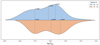 |
Fig. 1 Violin diagram of chromospheric-activity-level distribution for the stars in the sample. The vertical lines with their respective numbers indicate the values of the first, second, and third quartiles. Most of the stars in the sample show low levels of chromospheric emission indicating that most of them are inactive or very inactive. |
3.2 Surface-brightness study
To analyse the influence of stellar chromospheric activity on the surface brightness, we used the log  values obtained in the previous section and computed the surface brightness following the work of Salsi et al. (2021). To do this, we employed the values of the V and KS from SIMBAD and 2MASS, respectively (see Table 1).
The surface brightness F, defined by F = log Te f f + 0.1BC, is directly related to the bolometric correction (BC) and to the effective temperature (Te f f) of the star, and, therefore, to its colour (Wesselink 1969). According to Barnes & Evans (1976), the surface brightness in a given spectral band Fλ can be found from their apparent magnitude and their true apparent limb-darkened angular diameter θLD:
![Mathematical equation: $\[F_\lambda=C-0.1 m_{\lambda 0}-0.5 ~\log~ \theta_{L D},\]$](/articles/aa/full_html/2025/04/aa50348-24/aa50348-24-eq8.png) (1)
(1)
where mλ0 is the apparent magnitude corrected from the interstellar extinction. C is a constant depending on the Sun’s bolometric magnitude, Mbol; its total flux, f⊙; and the Stefan–Boltzmann constant, σ. For our study, we adopted C = 4.2196 according to the more accurate estimations of solar parameters (Mamajek et al. 2015; Prša et al. 2016).
On the other hand, the bolometric surface flux fbol of a star, which is expressed as the ratio between the bolometric flux Fbol and the squared limb-darkened angular diameter ![Mathematical equation: $\[\theta_{L D}^{2}\]$](/articles/aa/full_html/2025/04/aa50348-24/aa50348-24-eq9.png) , is linearly proportional to its effective temperature
, is linearly proportional to its effective temperature ![Mathematical equation: $\[T_{e f f}^{4}\]$](/articles/aa/full_html/2025/04/aa50348-24/aa50348-24-eq10.png) . It is thus also linearly linked to the colour mλ1 − mλ2. In this way, the surface brightness can be estimated by the following linear relation:
. It is thus also linearly linked to the colour mλ1 − mλ2. In this way, the surface brightness can be estimated by the following linear relation:
![Mathematical equation: $\[F_{\lambda 1}=a\left(m_{\lambda 1}-m_{\lambda 2}\right)_0+b,\]$](/articles/aa/full_html/2025/04/aa50348-24/aa50348-24-eq11.png) (2)
(2)
where the subscript 0 refers to the magnitudes corrected for interstellar extinction.
The interstellar attenuation AV in the visible band is defined as AV = RV × E(B − V), where RV is the total-to-selective extinction ratio in the visible band and E(B − V) is the B − V colour excess. To compute this, we used the Stilism5 online tool (Lallement et al. 2014; Capitanio et al. 2017), considering early Gaia DR3 distances (Gaia Collaboration 2023). The interest of this tool lies in the three-dimensional maps of local interstellar matter it provides, based on measurements of the starlight absorption by dust or gaseous species.
Taking all this into account and the angular diameters extracted from the literature (see Cols. 7 and 8 of Table 1), together with Eq. (1), we computed FV(θ) for the M dwarfs in the sample. On the other hand, we computed FV(V − KS) employing Eq. (2) and the colour indexes from Table 1. Finally, in Fig. 2 we show the possible influence of the chromospheric activity levels in the surface brightness by plotting the difference between the measured and calculated surface brightness (FV(θ) − FV(V − KS)) divided by the σRMS as a function of the chromospheric activity. Red crosses show the rejected stars by Salsi et al. (2021), black dots the targets considered by Salsi et al. (2021), and blue stars the new targets added in this work.
From our results, we can infer that there is no direct relationship between chromospheric activity and surface brightness in the domain of −5.6 < log ![Mathematical equation: $\[$R_{H K}^{\prime}$\]$](/articles/aa/full_html/2025/04/aa50348-24/aa50348-24-eq13.png) < −4.5. For the stars that are further away from 5σRMS, we found GJ 725 B and GJ 699, two objects that were discarded by Salsi et al. (2021) because the interferometric observations to derive the angular diameters were not the most suitable. However, there are other targets within the ±2.5σRMS range that were also rejected by Salsi et al. (2021). They rejected stars using different approaches, one of them related to interferometric criteria and stellar activity (fast rotators, spectroscopic binary, etc.) and photometry found in the literature. This preliminary study on the influence of chromospheric activity will continue soon on the basis of new interferometric observations (Mourard et al. 2022).
< −4.5. For the stars that are further away from 5σRMS, we found GJ 725 B and GJ 699, two objects that were discarded by Salsi et al. (2021) because the interferometric observations to derive the angular diameters were not the most suitable. However, there are other targets within the ±2.5σRMS range that were also rejected by Salsi et al. (2021). They rejected stars using different approaches, one of them related to interferometric criteria and stellar activity (fast rotators, spectroscopic binary, etc.) and photometry found in the literature. This preliminary study on the influence of chromospheric activity will continue soon on the basis of new interferometric observations (Mourard et al. 2022).
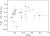 |
Fig. 2 Difference between measured and computed surface brightness in units of σRMS as a function of the log |

Synthesis of the characterisation and long-term activity analysis developed in this work.
3.3 Activity cycles
In order to look for some cyclical pattern in the magnetic activity of the stars in the sample, we constructed the S time series of each target containing at least five spectra. We have implemented the same colour code for all the time series in order to distinguish between the different instruments: blue for CASLEO spectra, orange for HARPS, green for FEROS, red for UVES, violet for X-shooter, brown for HIRES, yellow for HARPS-N, and light blue for ESPRESSO spectra. In this section, we show the time series for GJ 1 as an example of all the analysis implemented. For the rest of the stars that present a cyclical behaviour in their magnetic activity, we plotted the results in Appendix A.1, and stars without a cyclical pattern are shown in Appendix A.2. A summary of their characteristics as a number of observations used (Nobs) or an extension of the time series can be found in Cols. 2 and 3 of Table 2. We also cleaned them by discarding spectra that were possibly contaminated by transient events, such as flares, using the same criteria discussed in Ibañez Bustos et al. (2023) based on the distortion of the Balmer lines. In some time series, we highlight a few points with red circles to indicate that the spectral line could be contaminated by flares and that they were discarded from our analysis.
To characterise their activity based on decadal time series of each individual star, we also estimated the mean values of the Mount Wilson indexes (⟨S⟩) and their dispersion σS/⟨S⟩ as an estimation of the variability in the S series (see Cols. 4 and 5 of Table 2). For this purpose, we considered the non-flaring time series such that the values found were purely due to non-transient variability of the magnetic field.
To study the long-term magnetic activity and to know if it exhibits a cyclical behaviour or not, we searched for significant signals in the periodograms of the S series. For all of them, we employed the generalised Lomb-Scargle (GLS) periodogram (Zechmeister & Kürster 2009). To estimate the significance of the signals found in the periodograms, we took into account the false alarm probability (FAP) expressed in Ibañez Bustos et al. (2019a). To complement this, for stars with a significant FAP we also computed the bootstrap randomisation of the data following Endl et al. (2001) (see Col. 9 of Table 2). We define a significant signal as the frequencies whose power shows a FAP ≤ 0.1% in both of the above-mentioned methods.
Due to inhomogeneity and differences in the cadence of the time series or also due to the difference in sampling, several significant frequencies might appear in the periodograms. When the periodograms displayed numerous significant peaks, we proceeded in different ways; we binned the time series if the number of points was not well distributed over its time span or by subtracting the harmonic function fit associated with the most significant period(s) from the time series. We also considered two complementary tools: the Bayesian generalised Lomb–Scargle (BGLS) periodogram described in Mortier et al. (2015) and the CLEAN deconvolution algorithm developed by Roberts et al. (1987). When we needed to estimate the probability that a given frequency is related to an activity cycle, we calculated the BGLS; when we needed to discard frequencies from our periodograms due to, for example, aliasing induced by the spectral window function, we used the CLEAN algorithm.
We added the word potential or the word possible to specify that this is a first detection and not a confirmation of the activity cycle already reported in the literature. We detected 13 periodic signals that correspond to the first evidence of potential magnetic activity cycles6 and others already reported in the literature that we were able to confirm in this work. The error of the detected periods depends on the finite frequency resolution of their corresponding periodogram δν as given by Eq. (2) in Lamm et al. (2004): ![Mathematical equation: $\[\delta P=\frac{\delta \nu P^{2}}{2}\]$](/articles/aa/full_html/2025/04/aa50348-24/aa50348-24-eq17.png) . For stars where cyclical behaviour due to stellar magnetic activity was detected, we plotted the folded phases with their respective periods detected by the aforementioned periodograms. In each of these plots, we show the least-squares fit with a dashed red line, and the red shadow represents the ±3σ deviation.
. For stars where cyclical behaviour due to stellar magnetic activity was detected, we plotted the folded phases with their respective periods detected by the aforementioned periodograms. In each of these plots, we show the least-squares fit with a dashed red line, and the red shadow represents the ±3σ deviation.
We summarise the results of this section in Cols. 4–9 of Table 2. The analyses carried out for the different time series of the stars in the sample are listed below, and a detailed discussion of our results is shown in Sect. 4.
GJ 1 – HD 225213 – HIP 439. In Fig. 3, we show the time series and the results obtained from the GLS and BGLS periodograms. We find that the most significant peak corresponds to a period PGLS = (4286 ± 479) days with a FAP of ~0.0001. To corroborate that the 4286-day peak corresponds to an activity cycle and not an artefact or alias, we subtracted the harmonic function fit associated with this period from its time series and executed the GLS periodogram for the new residual series. We do not find any significant peaks in this step. On the other hand, to find the probability that this peak of ~4200 days corresponds to an activity cycle, we studied the BGLS periodogram (red curve in Fig. 3). From this analysis, we conclude that the peak associated with the 4286-day period corresponds to a potential activity cycle with a 99% probability for this partially convective star.
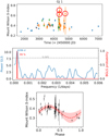
Fig. 3 GJ 1. Top: S-index time series. Middle: GLS periodogram (blue): (4286 ± 479) days with FAP = 0.01% and FAPbootstrap = 0.04%. BGLS periodogram (red): there is a probability of 99% that the peak of ~4200 days corresponds to a magnetic activity cycle for this star. Bottom: phase-folded time series with an ~4200 day period.
GJ 205 – HD 36395 – LHS 30. For this star, we executed GLS and CLEAN periodograms (see middle panel of Fig. A.1). For the S-index time series, a single significant peak stands out with a period of PGLS = 5313 ± 862 days and FAP < 0.1%; FAPbootstrap < 0.01% for the GLS periodogram and PCLEAN = 5479 ± 196 days for the CLEAN one. Both peaks would be associated with an activity cycle between 14.5 and 15 years for GJ 205. Subtracting the period of ~5400 days from our time series and running the periodograms again, we found no significant peaks. Thus, we conclude that the quiescent star GJ 205 has a potential magnetic activity cycle of ~5400 days.
GJ 229 A – HD 42581 – HIP 29295. In this study, by performing the GLS periodogram we obtained two significant peaks of PGLS;1 = 4949 ± 423 days and PGLS;2 = 123.2 ± 0.4 days, with FAPs of less than 0.1% (see middle panel of Fig. A.2). To analyse whether the PGLS;2 peak is a sampling effect, we executed the CLEAN periodogram, where we find the only significant signal at a period of PCLEAN = 4811 ± 150 days. Therefore, we discarded the fact that the 123-day peak is associated with modulations related to the activity of the star. We also analysed our time series with the BGLS periodogram and find that there is a 99% probability that the 4900-day peak is related to the activity cycle for our S series. In subtracting the 4900-day cycle from our series, we find no other significant peaks during the execution of the periodograms. We thus conclude that a cycle of ~13 yr is possibly modulating the magnetic activity cycle for this star. This cycle does not agree with those already reported in the literature; we discuss our results in Sect. 4.2.
GJ 393 – BD+01 2447 – HIP 51317. To study its long-term activity, we binned the time series every 30 days for those points in HJD > 6000 d in order to analyse a more homogeneous series. We calculated the GLS and CLEAN periodograms for the time series and obtained only two significant peaks with the GLS: PGLS;1 = (1124 ± 29) d and PGLS;2 = (274 ± 2) d with FAPs ~0.003% and ~0.04%, respectively (see middle panel of Fig. A.3). To know if the 274 peak is an alias, we executed the CLEAN periodogram. Only one significant frequency appears with a period of PCLEAN = (1112 ± 25) d and a FAPbootstrap = 0.02%. For this star, we conclude that GJ 393 presents a possible activity cycle of around 1100 days.
GJ 526 – HD 119850 – HIP 67155. In the middle panel of Fig. A.4, we show the GLS and CLEAN periodograms in which it is observed that there is a cyclic behaviour in the activity with a period of (3739 ± 288) days and a FAP of 0.013% and a FAPbootstrap = 0.08% for the GLS case (blue line), while for CLEAN (orange line) we obtained a period of (3115 ± 1336) days7. These results are in agreement with those reported by Suárez Mascareño et al. (2016). We thus conclude that GJ 526 exhibits a magnetic activity cycle of ~10 yr.
GJ 536 – HD 122303 – HIP 68469. We analysed the binned series with the GLS and CLEAN periodograms in Fig. A.5. In the case of the GLS periodogram, we found a peak corresponding to a period of (1643 ± 58) days with a FAP of 8 × 10⁻⁵; FAPbootstrap = 0.06%, while for the CLEAN case we found a period of (1667 ± 24) days. To search for other potential magnetic-activity cycles, we analysed the residuals of the series by subtracting the harmonic signal corresponding to the ~1600-day period. In this new residual series, we found a significant period peak of (4044 ± 443) days with a FAP of 0.05% (see bottom panel of Fig. A.5) and FAPbootstrap = 0.1%. When subtracting this new signal from our series, we did not detect any significant period. Finally, to corroborate our results, we worked with the original series without binning. Both cyclical signals are present in the unbinned series where we detected periods of 1643 ± 51 days and when subtracting this signal, one of 4382 ± 469 days, in both cases the FAPs < 0.1%. We therefore conclude that in this spectroscopic series, the period of ~1600 days is modulated by a larger activity cycle with a period of ~4000 days. This period is about twice as long as that reported by Suárez Mascareño et al. (2017). We discuss our results in Sect. 4.2.
-
GJ 551 – HIP 70890 – Proxima Centauri. In the top panel of Fig. A.6, we show the S-index time series followed by the GLS and CLEAN periodograms, where several peaks with high significance levels appear. These are as follows. GLS: PGLS;1 = (4946 ± 522) d, PGLS;2 = (110.6 ± 0.3) d, PGLS;3 = (81.5 ± 0.3) d con FAPs < 0.01%). CLEAN: PCLEAN;1 = (4226 ± 325) d and PCLEAN;2 = (81.5 ± 0.2) d.
As the rotational modulation of GJ 551 (~82 d, Kiraga & Stepien 2007) is present in the periodograms performed on our series, we subtracted the harmonic signal of ~82 days and ran the GLS periodogram to the new residual series. In this analysis, we obtained a single significant peak of PGLS = 4121 ± 321 days with a FAP of 0.0002 (see third panel of Fig. A.6) and FAPbootstrap = 0.05%. When we subtracted this signal from our series and ran the GLS periodogram, we did not obtain any other significant peaks. The magnetic activity of GJ 551 has already been studied, and its activity cycles have been reported in several works (Cincunegui et al. 2007; Wargelin et al. 2017). Our cycle of ~4000 days differs from those reported in the literature. We discuss our results in Sect. 4.2.
GJ 628 – BD-12 4523 – V* V2306 Oph. As the GLS periodogram displayed multiple peaks of high significance, we used the series binned every 30 days to study the long-term magnetic activity of this star. Using GLS and CLEAN, we obtained only one significant peak: PGLS = (4498 ± 607) d, with FAP of ~0.004%; FAPbootstrap = 0.01% and PCLEAN = (4153 ± 173) d, respectively (see middle panel of Fig. A.7). Finally, to corroborate our result we used the S series without binning, and with the GLS periodogram we obtained as the most significant peak a signal of PGLS = (4090 ± 363) d with a FAP ≪ 0.001%. We conclude that GJ 628 presents a potential activity cycle of ~4100 days.
GJ 699 – HIP 87937 – Barnard’s star. In Fig. A.8, we show the time series, the GLS and BGLS periodograms, and the phase for this target. The only significant period Pcyc = (3281 ± 255) d with a FAP of 1 × 10⁻⁵; FAPbootstrap = 0.02% would be related to the activity cycle with a probability of 96%. Toledo-Padrón et al. (2019) reported the rotation period for this star (Prot = 145 days) with an activity cycle of PmV = 3846.15 days using the ASAS photometric database, and a cycle of PS = 3225.81 days using spectroscopic data from seven different spectrographs. Our result is in line with that of Toledo-Padrón et al. (2019). However, we would like to point out that despite this, the S-index time series constructed in the present work does not show clear evidence of a periodic signal, as can also be seen in the plotted phase in Fig. A.8. Toledo-Padrón et al. (2019) used a modified S index constructed from the Ca II lines, so it is logical that the time series are not similar. Furthermore, it must be mentioned that the data used are not the same, and we did not find the peak related to the rotational modulation of ~145 days. Therefore, we conclude that despite having reproduced the potential cycle already detected by the aforementioned authors (~9 yr), this star should continue to be monitored for future analyses of the long-term magnetic activity.
GJ 752 A – HD 180617 – V V1428 Aql. To analyse its long-term magnetic activity, we implemented the GLS and CLEAN periodograms for the binned time series. The results are shown in the middle panel of Fig. A.9. We obtained only one significant peak: PGLS = (4416 ± 462) d with FAP < 0.01%; FAPbootstrap = 0.02% and PCLEAN = (4527 ± 174) d, respectively. When we removed this signal from our binned time series, we did not find another significant peak. We discuss our results in Sect. 4.2. We conclude that the magnetic activity of this star is possibly modulated by a cycle of ~12 years.
GJ 809 – HD 199305 – HIP 103096. To study its long-term activity, we calculated the GLS and CLEAN periodograms for the time series (see middle panel of Fig. A.10), and we obtained only one significant peak: PGLS = (2898 ± 273) d with FAP of ~0.001%; FAPbootstrap = 0.03% and PCLEAN = (2861 ± 79) d, respectively. The 418-day peak present in the GLS periodogram disappears in the CLEAN periodogram because it is probably related to an alias induced by the spectral window function. We thus conclude that this star exhibits a potential activity cycle of ~2800 days.
-
GJ 825 – HD 202560 – V* AX Mic. To study its long-term activity, we calculated the GLS periodogram, where we obtained two significant peaks: PGLS;1 = (7038 ± 2700) d and PGLS;2 = (365 ± 1) d with FAPs of 2 × 10⁻⁶ and 1 × 10⁻⁴, respectively (see second panel of Fig. A.11, blue line). To investigate whether the second peak associated with one year is related to an activity cycle or to a sampling effect, we computed the CLEAN periodogram. In the second panel of Fig. A.11, we show this periodogram with an orange line. Since the 365-day peak is not present in the CLEAN periodogram, we conclude that this peak is due to an alias induced by the spectral window function. On the other hand, we can observe that the largest peak still appears, and in this case its value is PCLEAN = (6078 ± 338) d.
Since the period of ~7000 days is longer than the time span of the sample (~5400 days), we studied the residual series obtained by subtracting the peak of ~7000 days from our S series. We show the results in the fourth panel of Fig. A.11; we found a single significant peak of PGLS = (2593 ± 137) d with a FAP of 0.04%; FAPbootstrap = 0.1% and PCLEAN = (2378 ± 104) days. Thus, we conclude that GJ 825 presents a possible activity cycle of ~2500 days that could be modulated by a higher peak of ~7000 days.
GJ 832 – HD 204961 – HIP 106440. To study its long-term activity, we calculated the GLS and CLEAN periodograms for the binned time series, and we obtained only one significant peak: PGLS = (2297 ± 54) d with FAP of 3 × 10⁻⁷; FAPbootstrap < 0.01% and PCLEAN = (2333 ± 49) d, respectively (see middle panel of Fig. A.12). We conclude that a cycle of ~6 years is potentially modulating the magnetic activity of this star.
3.4 Other M dwarfs
We did not detect any evidence of cyclical activities in the time series for the stars GJ 169, GJ 338 B, GJ 488, GJ 79, GJ 412 A, GJ 880, GJ 570 B, GJ 908, GJ 411, GJ 887, GJ 15 A, GJ 687, GJ 725 B, GJ 273, GJ 876, GJ 725 A, GJ 674, GJ 581, GJ 176, and GJ 406. The time series of these non-cyclical stars are plotted in Appendix A. They could be non-cyclic stars, or, in several cases, the time span or the sampling of the data set could be insufficient to detect a significant period. Thus, we need to keep observing this sample to build more reliable time series. It may also be due to the poor distribution and inhomogeneity of the points in the time series or simply because the stars have very low levels of chromospheric emission, which classifies them as very inactive and lacking magnetic-activity cycles. This is the case of GJ 273 (log  = −5.491 ± 0.063), which, with a large number of spectra approximately well distributed throughout the time series, does not present a cyclical behaviour in its magnetic activity due to the low variability of the star’s S index (see its time series in Appendix A).
Discarding GJ 406, in this stellar sample the mean value of the S index varies between 0.350 and 1.765, and the average variability and chromospheric emission level are around 12% and −5.110 dex, respectively. For the particular case of GJ 406, we found a variability of 90% in the S time series and the chromospheric emission level is the highest value in all the sample (log  = −3.986 ± 0.402). These values indicate that this star is very active with high chromospheric emission, and, therefore, considering the percentage of variability found, most of the spectra are possibly contaminated by flares. The way to improve this last issue in order to study the magnetic activity of this star is to observe it with a short cadence using both photometry and spectroscopy techniques.
For the particular case of GJ 581, the activity cycle was already reported by Gomes da Silva et al. (2012). They found a period of 3.85 years using the Na i spectral lines of HARPS spectra. Robertson et al. (2014) also studied the magnetic activity for this star and concluded that the ~1300 d-peak is the beat frequency of the 125- and 138-day signals associated with the rotation period, but, alternatively, the cycle may exist. In the present study, we used HARPS spectra with defined Ca II line emission where spectra with poor signal-to-noise ratios were discarded. Although Na I and Ca II indexes are not strictly correlated, due to different atmospheric sources responsible for the emission (Meunier et al. 2024) we also computed the Na I D index for our data set. Nevertheless, the data set used in this work is not exactly the same as the one used in Gomes da Silva et al. (2012). From our analysis, we were unable to find the 1300-day signal by using a similar data set through the S-index and Na I time series. Therefore, we conclude that this star should continue to be monitored for the analysis of its long-term magnetic activity and the possible confirmation of the activity cycle reported by the aforementioned works.
4 Discussions and conclusions
4.1 Surface-brightness study
In this work, we carried out an analysis of how magnetic activity in the stellar chromosphere of M dwarfs might have an impact on the surface brightness. As we mentioned in Sect. 3.2, it seems that there is no direct relationship between the two quantities, but this result is based on a small sample of targets.
The impact of the magnetic activity on the surface brightness and SBC relation is important; however, fundamentally, improving the SBCR for M dwarfs (even with for those stars with low magnetic activity levels) is necessary, as refinements are still required (as Kiman et al. 2024 recently quoted).
Our goal in the future is to improve the calibration of the surface brightness–colour relation in M dwarfs by using a larger sample. First of all, we must include more active stars in the sample since we currently only have three targets (GJ 338 B, GJ 729, and GJ 406) with values higher than log  = −4.5. To do so, we will have to observe these stars using interferometry to obtain their angular diameters directly, as only a few of them have been reported for M dwarfs. Once the CHARA/SPICA interferometer commissioning tests have been completed, we will be able to observe the M dwarfs, re-calibrate their SBCR, and, in particular, improve its robustness.
4.2 Activity cycles
From eight different spectroscopic databases, we built S-index time series for 31 of 35 dM stars in the sample presented in Appendix A. For those series with a time span longer than 4300 days, we computed GLS periodograms complemented by the BGLS and CLEAN periodograms and detected decadal and yearly cyclical patterns in 13 stars. These cycles have a duration between approximately three and 19 years. We also detected double cycles in three partially convective stars: GJ 536, GJ 825, and GJ 752 A. However, the periods detected for GJ 536, GJ 551, GJ 752 A, and GJ 229 A show discrepancies with those already reported in the literature. In the following paragraphs, we discuss a specific analysis on these targets.
For GJ 536, Suárez Mascareño et al. (2017) reported a period of 824.9 ± 1.7 days, which is about half what we found in this study. Suárez Mascareño et al. (2017) concluded that the periodicities detected when they analysed the Mount Wilson index and the Hα index may be apparent and close to the real periodicities caused by sampling, given that the series studied do not have an optimal extension to detect signals of prolonged periods. In this work, we used 216 spectra covering a time span of ~5800 days, implying that our S series is the longest series studied to date for this star, which shows a higher level of fidelity when searching for signals related to the magnetic activity cycle. We also studied the GJ 536 time series using the CLEAN algorithm, which allowed us to detect possible spurious signals due to sampling.
For GJ 551, Wargelin et al. (2017) reported an ~7-year magnetic-activity cycle for Proxima Centauri using ASAS photometry. It is important to note the different contributions depending on the observational technique used. On the one hand, photometry tracks starspots and filaments, while spectroscopy track plages related to local magnetic-field concentrations. The intensity of the emission of Ca II spectral lines increases with the fraction of non-thermal chromospheric heating that can be produced, for example by local magnetic inhomogeneities, thus providing a useful spectroscopic indicator to measure the intensity and area covered by magnetic fields. Recently, Suárez Mascareño et al. (2020) combined HARPS, UVES, and ESPRESSO spectroscopy; they detected no signals related to the possible magnetic activity cycle, concluding that any possible long-term variation is suppressed by the floating means of the different data sets. In our case, using only the 40 CASLEO spectra, we obtain a cycle of PGLS–CASLEO = (4121 ± 816) days and a FAP of 0.006, which is compatible with the result obtained in our previous analysis. Thus, we can conclude that our result is not affected by the different data sets used in our study; in fact, they complement each other. Finally, it is important to note the relevance of the discrimination in our study against spectra that may be contaminated by flares in this type of highly active star; among them, intensification and broadening in the Balmer lines – and in some cases in the Ca II lines – can be observed.
For GJ 752, Buccino et al. (2011) reported a magnetic activity cycle of seven years employing ASAS photometric data and the CASLEO spectroscopic data. On the other hand, Suárez Mascareño et al. (2016) detected an activity cycle of 9.3 years using a similar ASAS database. Our results are in disagreement with those reported in the literature. However, when we work with the series without binning, the most significant peak still appears to be ~4400 d. When this signal is discarded, the most significant period appears to be ~2500 d, similar to that reported in Buccino et al. (2011). We did not find this signal in our binned series despite the fact that our time series has an extension of more than 16 years. Therefore, we conclude that this star presents a magnetic activity modulated by an ~12 yr cycle in the time series of the chromospheric S index. It is important to emphasise that the cycles detected by photometry may not agree with those reported by chromospheric indicators for this kind of star. We therefore highlight that it is of great importance to pursue a more detailed study of the photospheric (spot) and chromospheric (plages) correlations in M stars.
With regard to GJ 229, Buccino et al. (2011) used the Ca K-line flux measured on flux-calibrated CASLEO spectra to obtain a magnetic activity cycle of 1649 days. On the other hand, Suárez Mascareño et al. (2016) and Díez Alonso et al. (2019) used ASAS photometric data to report an activity cycle of 8.3 years for this star (almost twice as long as the cycle found by Buccino et al. 2011). Recently, Mignon et al. (2023) measured the Hα line from HARPS spectra and detected a cycle of ~700 days. The time series used in these works have shorter extensions than the cycle we reported in the present work (~4900 days). Therefore, our results do not indicate incompatibility with what is reported in the literature, but we have the advantage of having studied a longer time series (~7700 d) with a larger number of spectra (86) than those of both authors.
There are other incompatibilities between our study and those from other authors, for example in the case of GJ 1. It is important to note that its rotation period (Prot = 60 d) was reported by Suárez Mascareño et al. (2015), where HARPS spectra were used for the analysis of the Ca II and Hα lines. More recently, Mignon et al. (2023) reported a rotation period of 91 days when studying the variability of Ca II, Na I, and Hα lines. In the present study, we did not find such modulation (see Fig. 3, middle), and therefore we conclude that a photometric analysis to corroborate the GJ 1 rotation period reported by Suárez Mascareño et al. (2015) and Mignon et al. (2023) is of great importance.
In conclusion, even for the study of long-term magnetic activity it is necessary to highlight the importance of high cadence photometric or spectroscopic studies to detect rotation periods in M dwarfs. Regarding the building of the time series, it is essential to have reliable series with a good temporal extension, taking into account that the discrimination of spectra that may be contaminated by transient events in this type of star is crucial. Finally, it is of great importance to study them with different techniques to mitigate sampling effects such as spurious signals or aliasing due to the spectral-window function.
Data availability
Table B.1 is available in electronic form at the CDS via anonymous ftp to cdsarc.cds.unistra.fr (130.79.128.5) or via https://cdsarc.cds.unistra.fr/viz-bin/cat/J/A+A/696/A230.
Acknowledgements
This project has received funding from the European Research Council (ERC) under the European Union’s Horizon 2020 research and innovation programme (Grant agreement No. 101019653).
Appendix A Time series
In this section we show the time series constructed in the present work for the stars in the sample. In Appendix A.1 we show the time series together with their periodograms and phases folded time series for those stars that show a cyclical behaviour in their activity that is possibly associated with a potential magnetic activity cycle. In Appendix A.2 we plot the time series for those stars that do not show a cyclical behaviour in their magnetic activity and we also present the time series for the stars GJ 729 and GJ 447 already reported in Ibañez Bustos et al. (2020) and Ibañez Bustos et al. (2019b), respectively.
The time series were constructed using our own observations from CASLEO and those public domain observations that we found in 7 different databases. To distinguish between the different instruments, we employed the same color code for all the time series constructed: blue for CASLEO spectra, orange for HARPS, green for FEROS, red for UVES, violet for XSHOOTER, brown for HIRES, yellow for HARPS-N and light blue for ESPRESSO spectra.
We have studied each spectrum in detail analysing the different spectral lines as we already suggest in Ibañez Bustos et al. (2023). In some of the following time series, we highlighted some points with red circles to indicate that the spectral line could be contaminated by flares and they were discarded from our analysis.
Appendix A.1 Stars with potential magnetic activity cycles
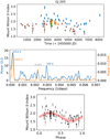 |
Fig. A.1 GJ 205. Top. S-Index time series. Middle. GLS and CLEAN periodograms: PGLS;1 = (5313 ± 862) d and PGLS;2 = 339 ± 3 d with a FAP < 0.01% and FAP ~ 0.001, respectively. From the CLEAN periodogram we have obtained as significant period PCLEAN = (5479 ± 196) days. Bottom. Phase folded time series with a ~5300 day period. |
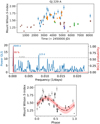 |
Fig. A.2 Same as Fig. 3 but for GJ 229 A. PGLS;1 = (4949 ± 423) d and PGLS;2 = (123.2 ± 0.4) d with FAPs < 0.1%. Performing the BGLS periodogram we obtained a 99% probability that the ~4900 d peak is present in our sample. Bottom. Phase folded time series with a ~4900 day period. |
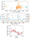 |
Fig. A.3 Same as Fig. A.1 but for GJ 393. PGLS;1 = (1124 ± 29) d and PGLS;2 = (274 ± 2) d with FAPs ~0.003 % and ~0.04 %, respectively. From the CLEAN periodogram we obtained a significant period of PCLEAN = (1112 ± 25) d. Bottom. Phase folded time series with a ~1100 day period. |
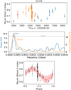 |
Fig. A.4 Same as Fig. A.1 for GJ 526. PGLS = (3739 ± 288) days with FAP of 0.013% and PCLEAN = (3115 ± 1336) days. Bottom. Phase folded time series with a ~3700 day period. |
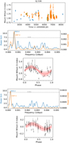 |
Fig. A.5 Same as Fig. A.1 but for GJ 536. PGLS = (1643 ± 58) days with a FAP of 8 × 10⁻⁵; CLEAN periodogram: (1667 ± 24) days. Third row. Phase folded time series with a ~1600 day period. Fourth row. GLS and CLEAN periodograms after substract the signal of ~1600-day peak, PGLS = 4044 ± 443 days with FAP of 0.05% and PCLEAN = 4167 ± 149 days. Bottom. Phase folded time series with a ~4100 day period. |
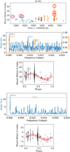 |
Fig. A.6 Same as Fig. A.1 but for GJ 551. GLS: PGLS;1 = (4946 ± 522) d, PGLS;2 = (110.6 ± 0.3) d, PGLS;3 = (81.5 ± 0.3) d con FAPs < 0.01%). CLEAN: PCLEAN;1 = (4226 ± 325) d and PCLEAN;2= (81.5 ± 0.2) d. Third row. Phase folded time series with a ~4900 day period. Fourth row. GLS and CLEAN periodograms after substract the signal of ~82-day peak, PGLS = 4121 ± 321 days with FAP of 0.0002. Bottom. Phase folded time series with a ~4100 day period. |
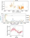 |
Fig. A.7 Same as Fig. A.1 but for GJ 628. GLS and CLEAN periodograms obtained for the time series binned every 30 days, PGLS = (4498 ± 607) d with FAP ~0.004 %. From the CLEAN periodogram we obtained a significant period of PCLEAN = (4153 ± 173) d. Bottom. Phase folded time series with a ~4400 day period. |
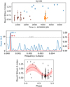 |
Fig. A.8 Same as Fig. 3 but for GJ 699. Pcyc = 3281 ± 255 days with FAP of 1 × 10⁻⁵ and a probability of 96% that the period correspond with the activity cycle for Gl 699. Bottom. Phase folded time series with a ~3300 day period. |
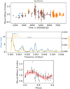 |
Fig. A.9 Same as Fig. A.1 but for GJ 752 A. PGLS = (4416 ± 462) d with FAP < 0.01% and PCLEAN = (4527 ± 174) d. Bottom. Phase folded time series with a ~4400 day period. |
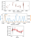 |
Fig. A.10 Same as Fig. A.1 but for GJ 809. PGLS;1 = (2898 ± 273) d and PGLS;2 = (418 ± 6) d with FAPs ~0.001 % and ~0.05 %, respectively. From the CLEAN periodogram we obtained a significant period of PCLEAN = (2861 ± 79) d. Bottom. Phase folded time series with a ~2900 day period. |
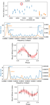 |
Fig. A.11 Same as Fig. A.1 but for GJ 825. PGLS;1 = (7038 ± 2700) d and PGLS;2 = (365 ± 1) d with FAPs of 2 × 10⁻⁶ and 1 × 10⁻⁴, respectively; CLEAN periodogram: PCLEAN = (6078 ± 338) d. Third row. Phase folded time series with a ~7000 day period. Fourth row. GLS and CLEAN periodograms after substract the ~7000-days peak, PGLS = (2593 ± 137) d with FAP 0.04% and PCLEAN = (2378 ± 104) d. Bottom. Phase folded time series with a ~2500 day period. |
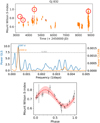 |
Fig. A.12 Same as Fig. A.1 but for GJ 832. PGLS = (2297 ± 54) d with FAP of 3 × 10⁻⁷ and PCLEAN = (2333 ± 49) d. Bottom. Phase folded time series with a ~2300 day period. |
Appendix A.2 Other M dwarfs
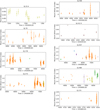 |
Fig. A.13 S-Index time series. |
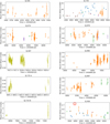 |
Fig. A.14 S-Index time series. |
References
- Astudillo-Defru, N., Delfosse, X., Bonfils, X., et al. 2017, A&A, 600, A13 [NASA ADS] [CrossRef] [EDP Sciences] [Google Scholar]
- Baliunas, S. L., Donahue, R. A., Soon, W. H., et al. 1995, ApJ, 438, 269 [Google Scholar]
- Barnes, T. G., & Evans, D. S. 1976, MNRAS, 174, 489 [Google Scholar]
- Berger, D. H., Gies, D. R., McAlister, H. A., et al. 2006, ApJ, 644, 475 [NASA ADS] [CrossRef] [Google Scholar]
- Bonfils, X., Delfosse, X., Udry, S., et al. 2013, A&A, 549, A109 [NASA ADS] [CrossRef] [EDP Sciences] [Google Scholar]
- Boyajian, T. S., von Braun, K., van Belle, G., et al. 2012, ApJ, 757, 112 [Google Scholar]
- Buccino, A. P., Lemarchand, G. A., & Mauas, P. J. D. 2007, Icarus, 192, 582 [NASA ADS] [CrossRef] [Google Scholar]
- Buccino, A. P., Díaz, R. F., Luoni, M. L., Abrevaya, X. C., & Mauas, P. J. D. 2011, AJ, 141, 34 [NASA ADS] [CrossRef] [Google Scholar]
- Buccino, A. P., Petrucci, R., Jofré, E., & Mauas, P. J. D. 2014, ApJ, 781, L9 [Google Scholar]
- Capitanio, L., Lallement, R., Vergely, J. L., Elyajouri, M., & Monreal-Ibero, A. 2017, A&A, 606, A65 [NASA ADS] [CrossRef] [EDP Sciences] [Google Scholar]
- Charbonneau, P. 2010, Liv. Rev. Sol. Phys., 7, 3 [Google Scholar]
- Cincunegui, C., & Mauas, P. J. D. 2004, A&A, 414, 699 [NASA ADS] [CrossRef] [EDP Sciences] [Google Scholar]
- Cincunegui, C., Díaz, R. F., & Mauas, P. J. D. 2007, A&A, 461, 1107 [NASA ADS] [CrossRef] [EDP Sciences] [Google Scholar]
- Cosentino, R., Lovis, C., Pepe, F., et al. 2012, SPIE Conf. Ser., 8446, 84461V [Google Scholar]
- Dekker, H., D’Odorico, S., Kaufer, A., Delabre, B., & Kotzlowski, H. 2000, SPIE Conf. Ser., 4008, 534 [Google Scholar]
- Di Benedetto, G. P. 2005, MNRAS, 357, 174 [NASA ADS] [CrossRef] [Google Scholar]
- Di Maio, C., Argiroffi, C., Micela, G., et al. 2020, A&A, 642, A53 [NASA ADS] [CrossRef] [EDP Sciences] [Google Scholar]
- Díaz, R. F., González, J. F., Cincunegui, C., & Mauas, P. J. D. 2007, A&A, 474, 345 [NASA ADS] [CrossRef] [EDP Sciences] [Google Scholar]
- Díez Alonso, E., Caballero, J. A., Montes, D., et al. 2019, A&A, 621, A126 [NASA ADS] [CrossRef] [EDP Sciences] [Google Scholar]
- Dressing, C. D., & Charbonneau, D. 2015, ApJ, 807, 45 [Google Scholar]
- Duncan, D. K., Vaughan, A. H., Wilson, O. C., et al. 1991, ApJS, 76, 383 [Google Scholar]
- Endl, M., Kürster, M., Els, S., Hatzes, A. P., & Cochran, W. D. 2001, A&A, 374, 675 [NASA ADS] [CrossRef] [EDP Sciences] [Google Scholar]
- Flores, M., González, J. F., Jaque Arancibia, M., Buccino, A., & Saffe, C. 2016, A&A, 589, A135 [NASA ADS] [CrossRef] [EDP Sciences] [Google Scholar]
- Flores, M., González, J. F., Jaque Arancibia, M., et al. 2018, A&A, 620, A34 [NASA ADS] [CrossRef] [EDP Sciences] [Google Scholar]
- Gaia Collaboration (Vallenari, A., et al.) 2023, A&A, 674, A1 [NASA ADS] [CrossRef] [EDP Sciences] [Google Scholar]
- Gaidos, E., Mann, A. W., Lépine, S., et al. 2014, MNRAS, 443, 2561 [Google Scholar]
- Gent, M. R., Bergemann, M., Serenelli, A., et al. 2022, A&A, 658, A147 [NASA ADS] [CrossRef] [EDP Sciences] [Google Scholar]
- Gomes da Silva, J., Santos, N. C., Bonfils, X., et al. 2011, A&A, 534, A30 [NASA ADS] [CrossRef] [EDP Sciences] [Google Scholar]
- Gomes da Silva, J., Santos, N. C., Bonfils, X., et al. 2012, A&A, 541, A9 [NASA ADS] [CrossRef] [EDP Sciences] [Google Scholar]
- Günther, M. N., Zhan, Z., Seager, S., et al. 2020, AJ, 159, 60 [Google Scholar]
- Ibañez Bustos, R. V., Buccino, A. P., Flores, M., et al. 2019a, MNRAS, 483, 1159 [CrossRef] [Google Scholar]
- Ibañez Bustos, R. V., Buccino, A. P., Flores, M., & Mauas, P. J. D. 2019b, A&A, 628, L1 [NASA ADS] [CrossRef] [EDP Sciences] [Google Scholar]
- Ibañez Bustos, R. V., Buccino, A. P., Messina, S., Lanza, A. F., & Mauas, P. J. D. 2020, A&A, 644, A2 [NASA ADS] [CrossRef] [EDP Sciences] [Google Scholar]
- Ibañez Bustos, R. V., Buccino, A. P., Flores, M., Martinez, C. F., & Mauas, P. J. D. 2023, A&A, 672, A37 [NASA ADS] [CrossRef] [EDP Sciences] [Google Scholar]
- Kaufer, A., Stahl, O., Tubbesing, S., et al. 1999, The Messenger, 95, 8 [Google Scholar]
- Kervella, P., Thévenin, F., Di Folco, E., & Ségransan, D. 2004, A&A, 426, 297 [NASA ADS] [CrossRef] [EDP Sciences] [Google Scholar]
- Kiman, R., Brandt, T. D., Faherty, J. K., & Popinchalk, M. 2024, AJ, 168, 126 [Google Scholar]
- Kiraga, M., & Stepien, K. 2007, Acta Astron., 57, 149 [NASA ADS] [Google Scholar]
- Lafarga, M., Ribas, I., Reiners, A., et al. 2021, A&A, 652, A28 [NASA ADS] [CrossRef] [EDP Sciences] [Google Scholar]
- Lallement, R., Vergely, J. L., Valette, B., et al. 2014, A&A, 561, A91 [NASA ADS] [CrossRef] [EDP Sciences] [Google Scholar]
- Lamm, M. H., Bailer-Jones, C. A. L., Mundt, R., Herbst, W., & Scholz, A. 2004, A&A, 417, 557 [NASA ADS] [CrossRef] [EDP Sciences] [Google Scholar]
- Ligi, R., Creevey, O., Mourard, D., et al. 2016, A&A, 586, A94 [NASA ADS] [CrossRef] [EDP Sciences] [Google Scholar]
- Lovis, C., Dumusque, X., Santos, N. C., et al. 2011, arXiv e-prints [arXiv:1107.5325] [Google Scholar]
- Mamajek, E. E., Torres, G., Prsa, A., et al. 2015, arXiv e-prints [arXiv:1510.06262] [Google Scholar]
- Mayor, M., Pepe, F., Queloz, D., et al. 2003, The Messenger, 114, 20 [NASA ADS] [Google Scholar]
- Meunier, N., Mignon, L., Kretzschmar, M., & Delfosse, X. 2024, A&A, 684, A106 [NASA ADS] [CrossRef] [EDP Sciences] [Google Scholar]
- Mignon, L., Meunier, N., Delfosse, X., et al. 2023, A&A, 675, A168 [NASA ADS] [CrossRef] [EDP Sciences] [Google Scholar]
- Miguel, Y., Kaltenegger, L., Linsky, J. L., & Rugheimer, S. 2015, MNRAS, 446, 345 [Google Scholar]
- Mortier, A., Faria, J. P., Correia, C. M., Santerne, A., & Santos, N. C. 2015, A&A, 573, A101 [NASA ADS] [CrossRef] [EDP Sciences] [Google Scholar]
- Mourard, D., Nardetto, N., ten Brummelaar, T., et al. 2018, SPIE Conf. Ser., 10701, 1070120 [NASA ADS] [Google Scholar]
- Mourard, D., Berio, P., Pannetier, C., et al. 2022, SPIE Conf. Ser., 12183, 1218308 [NASA ADS] [Google Scholar]
- Newton, E. R., Irwin, J., Charbonneau, D., et al. 2017, ApJ, 834, 85 [Google Scholar]
- Pannetier, C., Mourard, D., Berio, P., et al. 2020, SPIE Conf. Ser., 11446, 114460T [NASA ADS] [Google Scholar]
- Pepe, F., Cristiani, S., Rebolo, R., et al. 2021, A&A, 645, A96 [NASA ADS] [CrossRef] [EDP Sciences] [Google Scholar]
- Prša, A., Harmanec, P., Torres, G., et al. 2016, AJ, 152, 41 [Google Scholar]
- Rabus, M., Lachaume, R., Jordán, A., et al. 2019, MNRAS, 484, 2674 [Google Scholar]
- Rauer, H., Catala, C., Aerts, C., et al. 2014, Exp. Astron., 38, 249 [Google Scholar]
- Rauer, H., Aerts, C., Cabrera, J., et al. 2024, arXiv e-prints [arXiv:2406.05447] [Google Scholar]
- Roberts, D. H., Lehar, J., & Dreher, J. W. 1987, AJ, 93, 968 [Google Scholar]
- Robertson, P., Mahadevan, S., Endl, M., & Roy, A. 2014, Science, 345, 440 [Google Scholar]
- Rodríguez Martínez, R., Lopez, L. A., Shappee, B. J., et al. 2020, ApJ, 892, 144 [NASA ADS] [CrossRef] [Google Scholar]
- Salsi, A., Nardetto, N., Mourard, D., et al. 2020, A&A, 640, A2 [NASA ADS] [CrossRef] [EDP Sciences] [Google Scholar]
- Salsi, A., Nardetto, N., Mourard, D., et al. 2021, A&A, 652, A26 [NASA ADS] [CrossRef] [EDP Sciences] [Google Scholar]
- Salsi, A., Nardetto, N., Plez, B., & Mourard, D. 2022, A&A, 662, A120 [NASA ADS] [CrossRef] [EDP Sciences] [Google Scholar]
- Schaefer, G. H., White, R. J., Baines, E. K., et al. 2018, ApJ, 858, 71 [Google Scholar]
- Ségransan, D., Kervella, P., Forveille, T., & Queloz, D. 2003, A&A, 397, L5 [NASA ADS] [CrossRef] [EDP Sciences] [Google Scholar]
- Suárez Mascareño, A., Rebolo, R., González Hernández, J. I., & Esposito, M. 2015, MNRAS, 452, 2745 [Google Scholar]
- Suárez Mascareño, A., Rebolo, R., & González Hernández, J. I. 2016, A&A, 595, A12 [Google Scholar]
- Suárez Mascareño, A., González Hernández, J. I., Rebolo, R., et al. 2017, A&A, 597, A108 [NASA ADS] [CrossRef] [EDP Sciences] [Google Scholar]
- Suárez Mascareño, A., Faria, J. P., Figueira, P., et al. 2020, A&A, 639, A77 [Google Scholar]
- Toledo-Padrón, B., González Hernández, J. I., Rodríguez-López, C., et al. 2019, MNRAS, 488, 5145 [Google Scholar]
- Vernet, J., Dekker, H., D’Odorico, S., et al. 2011, A&A, 536, A105 [NASA ADS] [CrossRef] [EDP Sciences] [Google Scholar]
- Vida, K., Kővári, Z., Pál, A., Oláh, K., & Kriskovics, L. 2017, ApJ, 841, 124 [Google Scholar]
- Vogt, S. S., Allen, S. L., Bigelow, B. C., et al. 1994, in Instrumentation in Astronomy VIII, 2198, eds. D. L. Crawford, & E. R. Craine, International Society for Optics and Photonics (SPIE), 362 [Google Scholar]
- Wargelin, B. J., Saar, S. H., Pojmański, G., Drake, J. J., & Kashyap, V. L. 2017, MNRAS, 464, 3281 [NASA ADS] [CrossRef] [Google Scholar]
- Wesselink, A. J. 1969, MNRAS, 144, 297 [NASA ADS] [CrossRef] [Google Scholar]
- Wright, N. J., & Drake, J. J. 2016, Nature, 535, 526 [Google Scholar]
- Wright, N. J., Drake, J. J., Mamajek, E. E., & Henry, G. W. 2011, ApJ, 743, 48 [Google Scholar]
- Wright, N. J., Newton, E. R., Williams, P. K. G., Drake, J. J., & Yadav, R. K. 2018, MNRAS, 479, 2351 [Google Scholar]
- Zechmeister, M., & Kürster, M. 2009, A&A, 496, 577 [CrossRef] [EDP Sciences] [Google Scholar]
The habitable zone is defined as the region in the equatorial plane of the star where water in the planet, if there is any, can be found in its liquid state.
The online tool is available at http://stilism.obspm.fr
We added the word ‘potential’ or the word ‘possible’ to distinguish that this is a first detection and not a confirmation of the activity cycle already reported in the literature.
Here, the error was computed as the HWHM×P2, where P is the period found.
All Tables
Synthesis of the characterisation and long-term activity analysis developed in this work.
All Figures
|
Fig. 1 Violin diagram of chromospheric-activity-level distribution for the stars in the sample. The vertical lines with their respective numbers indicate the values of the first, second, and third quartiles. Most of the stars in the sample show low levels of chromospheric emission indicating that most of them are inactive or very inactive. |
| In the text | |
|
Fig. 2 Difference between measured and computed surface brightness in units of σRMS as a function of the log |
| In the text | |
|
Fig. 3 GJ 1. Top: S-index time series. Middle: GLS periodogram (blue): (4286 ± 479) days with FAP = 0.01% and FAPbootstrap = 0.04%. BGLS periodogram (red): there is a probability of 99% that the peak of ~4200 days corresponds to a magnetic activity cycle for this star. Bottom: phase-folded time series with an ~4200 day period. |
| In the text | |
|
Fig. A.1 GJ 205. Top. S-Index time series. Middle. GLS and CLEAN periodograms: PGLS;1 = (5313 ± 862) d and PGLS;2 = 339 ± 3 d with a FAP < 0.01% and FAP ~ 0.001, respectively. From the CLEAN periodogram we have obtained as significant period PCLEAN = (5479 ± 196) days. Bottom. Phase folded time series with a ~5300 day period. |
| In the text | |
|
Fig. A.2 Same as Fig. 3 but for GJ 229 A. PGLS;1 = (4949 ± 423) d and PGLS;2 = (123.2 ± 0.4) d with FAPs < 0.1%. Performing the BGLS periodogram we obtained a 99% probability that the ~4900 d peak is present in our sample. Bottom. Phase folded time series with a ~4900 day period. |
| In the text | |
|
Fig. A.3 Same as Fig. A.1 but for GJ 393. PGLS;1 = (1124 ± 29) d and PGLS;2 = (274 ± 2) d with FAPs ~0.003 % and ~0.04 %, respectively. From the CLEAN periodogram we obtained a significant period of PCLEAN = (1112 ± 25) d. Bottom. Phase folded time series with a ~1100 day period. |
| In the text | |
|
Fig. A.4 Same as Fig. A.1 for GJ 526. PGLS = (3739 ± 288) days with FAP of 0.013% and PCLEAN = (3115 ± 1336) days. Bottom. Phase folded time series with a ~3700 day period. |
| In the text | |
|
Fig. A.5 Same as Fig. A.1 but for GJ 536. PGLS = (1643 ± 58) days with a FAP of 8 × 10⁻⁵; CLEAN periodogram: (1667 ± 24) days. Third row. Phase folded time series with a ~1600 day period. Fourth row. GLS and CLEAN periodograms after substract the signal of ~1600-day peak, PGLS = 4044 ± 443 days with FAP of 0.05% and PCLEAN = 4167 ± 149 days. Bottom. Phase folded time series with a ~4100 day period. |
| In the text | |
|
Fig. A.6 Same as Fig. A.1 but for GJ 551. GLS: PGLS;1 = (4946 ± 522) d, PGLS;2 = (110.6 ± 0.3) d, PGLS;3 = (81.5 ± 0.3) d con FAPs < 0.01%). CLEAN: PCLEAN;1 = (4226 ± 325) d and PCLEAN;2= (81.5 ± 0.2) d. Third row. Phase folded time series with a ~4900 day period. Fourth row. GLS and CLEAN periodograms after substract the signal of ~82-day peak, PGLS = 4121 ± 321 days with FAP of 0.0002. Bottom. Phase folded time series with a ~4100 day period. |
| In the text | |
|
Fig. A.7 Same as Fig. A.1 but for GJ 628. GLS and CLEAN periodograms obtained for the time series binned every 30 days, PGLS = (4498 ± 607) d with FAP ~0.004 %. From the CLEAN periodogram we obtained a significant period of PCLEAN = (4153 ± 173) d. Bottom. Phase folded time series with a ~4400 day period. |
| In the text | |
|
Fig. A.8 Same as Fig. 3 but for GJ 699. Pcyc = 3281 ± 255 days with FAP of 1 × 10⁻⁵ and a probability of 96% that the period correspond with the activity cycle for Gl 699. Bottom. Phase folded time series with a ~3300 day period. |
| In the text | |
|
Fig. A.9 Same as Fig. A.1 but for GJ 752 A. PGLS = (4416 ± 462) d with FAP < 0.01% and PCLEAN = (4527 ± 174) d. Bottom. Phase folded time series with a ~4400 day period. |
| In the text | |
|
Fig. A.10 Same as Fig. A.1 but for GJ 809. PGLS;1 = (2898 ± 273) d and PGLS;2 = (418 ± 6) d with FAPs ~0.001 % and ~0.05 %, respectively. From the CLEAN periodogram we obtained a significant period of PCLEAN = (2861 ± 79) d. Bottom. Phase folded time series with a ~2900 day period. |
| In the text | |
|
Fig. A.11 Same as Fig. A.1 but for GJ 825. PGLS;1 = (7038 ± 2700) d and PGLS;2 = (365 ± 1) d with FAPs of 2 × 10⁻⁶ and 1 × 10⁻⁴, respectively; CLEAN periodogram: PCLEAN = (6078 ± 338) d. Third row. Phase folded time series with a ~7000 day period. Fourth row. GLS and CLEAN periodograms after substract the ~7000-days peak, PGLS = (2593 ± 137) d with FAP 0.04% and PCLEAN = (2378 ± 104) d. Bottom. Phase folded time series with a ~2500 day period. |
| In the text | |
|
Fig. A.12 Same as Fig. A.1 but for GJ 832. PGLS = (2297 ± 54) d with FAP of 3 × 10⁻⁷ and PCLEAN = (2333 ± 49) d. Bottom. Phase folded time series with a ~2300 day period. |
| In the text | |
|
Fig. A.13 S-Index time series. |
| In the text | |
|
Fig. A.14 S-Index time series. |
| In the text | |
Current usage metrics show cumulative count of Article Views (full-text article views including HTML views, PDF and ePub downloads, according to the available data) and Abstracts Views on Vision4Press platform.
Data correspond to usage on the plateform after 2015. The current usage metrics is available 48-96 hours after online publication and is updated daily on week days.
Initial download of the metrics may take a while.